Review

Valuation of Long-Term Investments in Energy Assets under Uncertainty

Bilbao Bizkaia Kutxa, Gran V´ıa 30, 48009 Bilbao, Spain
Energies 2009, 2(3), 738-768; https://doi.org/10.3390/en20300738
Submission received: 5 August 2009 / Accepted: 2 September 2009 / Published: 4 September 2009
(This article belongs to the Special Issue Energy Economics)

Abstract

:
This paper aims to contribute to the development of valuation models for long-term investments while keeping an eye on market prices. The adopted methodology is rooted on the existence of markets for futures and options on commodities related to energy investments. These markets are getting ever-increasingly liquid with ever-longer maturities while trading contracts. We discuss the advantages of this approach relative to other alternatives such as the Net Present Value (NPV) or the Internal Rate of Return (IRR), despite a limited increase in the complexity of the models involved. More specifically, using the valuation methods well-known to energy-finance academics, the paper shows how to: break down an investment into its constituent parts, apply to each of them the corresponding risk premium, value annuities on assets with a deterministic or stochastic behavior, and value the options that are available to its owner, in order to get an overall value of the investment project. It also includes an application to improvement in coal consumption, where futures markets are used to get a numerical estimate of the parameters that are required for valuation. The results are then compared with those from traditional methodologies. Conclusions for this type of investments under uncertainty are derived.

1. Introduction

Investments in energy assets are characterized by several relevant features. Among them we emphasize: large sums of money, non-negligible construction periods, long useful lives, uncertainty (financial, technical, regulatory, ...), maintenance costs. Given the size of the resources committed in the investments, the huge funding needs until the first revenues arise, and the long useful life of the facilities, it is necessary to have a suitable valuation method. Also, we must be aware of the advantages and shortcomings of each method.
When investing in energy assets, either revenues or costs or both of them depend on the quantities of commodities produced and consumed. Commodities prices are typically established in spot and futures markets. These prices and other issues1 are subject to uncertainty, which renders the valuation model particularly important. A faulty assessment of uncertainty can lead to wrong investment decisions. Thus, using a (unduly) higher risk premium can push managers to reject (relatively) less risky investments; and using a (unduly) lower risk premium can push them to accept (relatively) more risky investments.
In order to value these investments, a number of traditional methods are usually adopted. Among them we can mention the life-cycle cost analysis, simple or discounted payback, benefit cost analysis (BCA), net present value (NPV) and internal rate-of-return (IRR). The life-cycle cost analysis computes the discounted costs of construction, acquisition, maintenance and operation over a period of time. This methodology can be accessed in McCardell [1] and Bhattacharjee [2]. The payback period is the number of years until revenues exceed the initial disbursement.
These methods, however, typically fail to grapple with the project’s uncertainty in a satisfactory way. Besides, they make little or no use of spot and futures prices. Nonetheless, a model developed from the NPV, as the one in this paper, can correctly cope with uncertainty in the absence of flexibilities or options.
McDonald [3] analyzes to what extent rules of thumb such as payback and hurdle rates can approach the true value of an investment regarding projects with options under uncertainty. But this would be more appropriate in the case of small firms according to Graham and Harvey [4]; as they show, both the IRR and the NPV are used very frequently. These methods are even the most used methods, despite the supremacy that the capital-budgeting literature acknowledges to methods of valuation under uncertainty. In particular, the article by Graham and Harvey collets the results from a survey that has been responded by 392 chief financial officers. They find that 74.9% always or almost always use NPV, while 75.7% always or almost always use IRR. This report also shows that a large number of firms use company-wide discount rates to evaluate projects rather than project-specific discount rates.
There is a sizeable body of literature on valuation of derivative assets such as futures and options on financial assets or commodities. However, this literature tends to be focused on short-term operations; see for instance Wilmott [5]. Among the works on investment in real assets under uncertainty (or Real Options (RO) valuation) we mention the books by Dixit and Pindyck [6], and Trigeorgis [7]. Applications of this approach to the energy sector can be found in Ronn [8]. There is also a series of papers presented at the yearly international conference on Real Options which are available at http://www.realoptions.org/index.html.
More specifically, there are several papers on valuation of generation assets, some of which are cited here. Rocha et al. [9] analyze the competitiveness of a thermal power plant in Brazil. Gollier et al. [10] address the value of modularity in the choice between a large nuclear power plant and a flexible sequence of nuclear power plants. Näsäkkälä and Fleten [11] value a gas-fired power plant using a two-factor model for the spark spread. They apply this model to a base load power plant computing the optimal time to build. They also apply it to assess the possibility to upgrade this plant, at a cost, to a peak load plant. Abadie and Chamorro [12] analyze the choice between a base load gas-fired power plant and an integrated gasification combined cycle (IGCC) which operates in a flexible way (burning either coal or natural gas) using the cheapest fuel; they derive the optimal fuel prices to invest. Abadie and Chamorro [13] address the valuation of a base load natural gas combined cycle power plant (NGCC) and a liquefied natural gas (LNG) facility with several American-type investment options following the least squares Monte Carlo approach. Deng [14], starting from futures contracts on electricity and natural gas, values generation and transmission assets. First he assumes a standard geometric Brownian motion (GBM) and then a mean-reverting model. Deng [15] extends the former model to allow for jumps and spikes in prices.
This paper deals with investments in a long-lived real asset that consumes or produces a regular flow of commodities (measured in physical units) over its useful life. This would be the case of a power plant operating as a base load plant or investments to enhance energy efficiency. These flows of actual revenues and expenses will depend on the spot market prices over its useful life. And the risk of these flows will determine their valuation at the current time.
Even without any embedded options (which are addressed by RO analysis), the valuation of this type of investments depends on market prices. Thus, as a first step we need a stochastic cash flows valuation model that is consistent with the markets. Then it will be possible to value options by applying this valuation model to the process that governs commodity prices in the risk-neutral world. This can be accomplished by means of the numerical methods that are usual in the RO approach. Among them we have binomial lattices, Monte Carlo simulation, and finite difference methods.
The paper is organized as follows. Section 2 introduces the valuation model that we develop starting from the NPV. Section 3 discusses the most relevant issues for valuation. Some diffusion models for price dynamics are analyzed in Section 4, along with the formulas for valuation of futures contracts and stochastic cash flows, and the consequences of parameter values on the risk of these investments. Then in Section 5 we address modeling issues such as seasonality, the existence of jumps, and stochastic volatility with mean reversion; despite being very important in short-term derivatives, they have a very limited impact on the valuation of long-term stochastic cash flows. While the behavior of the long-run equilibrium price level is very important for valuation, Section 6 assesses an improvement in energy efficiency that saves coal consumption by using the former concepts. Section 7 concludes.

2. Development of the NPV for Valuing Stochastic Cash Flows

Traditionally several possible scenarios are considered. For each scenario, the cash flows at any time are computed and subsequently discounted to the present. The overall sum of all discounted flows in each scenario yields the NPV. More sophisticated analysis adopt a probabilistic distribution of scenarios to derive the expected net present value (ENPV) of those scenarios. The expected value of the cash flows is sometimes difficult to compute. In the case of a GBM this problem is particularly severe if we try to get the drift rate from historical prices. As shown by Gourieroux and Jasiak [16], it is very difficult to estimate the drift rate with any confidence. Therefore, it may not be convenient to make an ENPV-based valuation in some cases, among them the GBM.
There are several problems for computing the NPV; some of them are mentioned below.

2.1. The discount rate

This is a first problem since typically, and incorrectly, it is kept constant for valuing several projects which may face different risks. Indeed a constant rate does not take into account that uncertainty can unfold over time and that managers may be able to make decisions that mitigate risk at a future moment. Sometimes the firm’s weighted after-tax cost of capital is used; this is given by the following formula:
r D ( 1 - t a x ) D + r E E D + E
where r D is the interest rate on the debt, r E is the expected return on equity, and t a x is the marginal tax rate; D and E denote the amount of debt and equity, respectively. Yet this method will only be suitable if the projects to be assessed involve a risk which is similar to the firm’s risk2.
A unique discount rate is usually computed. This is a hard problem when we want to get a reliable estimate which is consistent with the project’s risks. Obviously, the riskier the investment project, the higher the discount rate. This applies whatever the source of uncertainty can be (financial, regulatory, technological, ...). In the particular case of energy assets (with long useful lives), the appropriate discount rate is a relevant issue for the choice of a valuation methodology which better fits the risks of each investment project3.
Note also that in some projects the risks can at least partially offset. Consider the case of natural gas-fired combined cycles (NGCC). If these power plants are the marginal plants that set the price in electricity markets, this price will somehow mirror their costs. Thus, they will enjoy a relatively stable profit margin (or spark spread) which renders them as relatively less risky investments (at least as long as they continue to be the marginal technology most of the time, or their average cost is very close to the marginal price whatsoever). In this case, though both commodities (electricity and natural gas) involve significant price risk, their combination in an NGCC power plant exhibits a lower risk; this should be duly considered in the valuation process.
Though the formula including the discounted cash flows is relatively simple, the computation of the correct discount rate is a very complex issue. This issue can be avoided by adopting an alternative valuation method, as described in this paper. It is based on grouping the deterministic cash flows (discounted at the risk-free rate) and the stochastic cash flows sorted by markets and evaluating them according to these markets’ prices. This approach sidesteps the problem of the discount rate, which is no longer necessary to compute4, and is consistent with the risk profile of the project5.
Example. Consider a project with fixed earnings F E t at time t, assumed to be received at the end of the year. There are also stochastic revenues perceived at t from producing amounts O U t i of the output (measured in energy units) which are related to a number of markets i = 1 , . . , k . Fixed costs are denoted by F C t . Stochastic costs incurred by consuming I N t j inputs (measured in physical units) are related to markets j = 1 , . . , l . We assume that there are enough futures markets or that we can compute futures prices F i ( S 0 i , t ) and F j ( S 0 j , t ) for delivery at time t of the goods involved; superscripts refer to the specific market, and S 0 stands for the time-0 spot price in these markets. In this case, assuming there is no option embedded in the project, its value over n years is given by:
t = 0 n F E t ( 1 + r f ) t + k i = 1 n t = 0 O U t i F i ( S 0 i , t ) ( 1 + r f ) t - t = 0 n F C t ( 1 + r f ) t - l j = 1 n t = 0 I N t j F j ( S 0 j , t ) ( 1 + r f ) t
After multiplying the physical quantities by their futures prices, these sums are discounted at the risk-free rate r f 6. It is the possibility to hedge these cash flows at these prices in futures markets that allows this type of valuation.
In this example, F E t , F C t and r f are deterministic, while the revenues from the output and the costs from consumption are stochastic. Yet the latter have a present value according to futures prices and the interest rate r f .
Everything rests on the existence of futures markets with the required maturities, where prices reflect the risk premium prevailing in the market. If contracts with the desired maturities are not available, we can estimate a mathematical model and assume that it will continue to hold over longer time horizons. Alternatively, it can be estimated with prices from another futures market with longer maturities which is highly correlated with the market of our interest; Cortazar et al. [17] propose a methodology to estimate the behavior of a commodity price in terms of another’s.
If expenses and revenues from the commodities are incurred continuously over time another formulation can be used. In the simple case of one input and one output with stochastic prices, we have:
O U 0 n e - r t F O U ( t , 0 ) d t - I N 0 n e - r t F I N ( t , 0 ) d t + n t = 0 F E t e - r t - n t = 0 F C t e - r t
where O U denotes the amount produced yearly, I N is the amount consumed yearly, and F O U ( t , 0 ) and F I N ( t , 0 ) stand for their respective time-0 prices in the futures markets for delivery at t. These prices are discounted at the continuous risk-free rate r. Deterministic cash flows are assumed to be received at discrete times.

2.2. Optionality

The flexibilities or options available to the manager of a particular project can be of different types. Trigeorgis [7] distinguishes: option to defer, time-to-build option, option to alter operating scale, option to abandon, option to switch, growth options, and multiple interacting options. In principle, for valuation purposes the most relevant ones for the project at hand should be addressed. For example, there can be an option to temporarily close down the plant, or to abandon it permanently, if revenues do not cover variable costs (e.g., fuel costs). These options must be valued taking into account the potential costs to switching from one state to another (open, moth-balled, abandoned) and the probability that the project becomes again profitable in the future. Optionality is very hard to grasp in NPV computations with a unique discount rate.
One of the first duties should always be to identify the options embedded in a given investment project. For example, the option to wait in a project to improve energy efficiency, the option to undertake investment on a modular basis, etc. The type of options will depend on the intrinsic characteristics of the project. But the project design itself can be made more flexible, which renders the project more valuable for the manager.
When there are options the value of an investment V at the initial time can be expressed as:
V = V I + R O
where V I denotes the value of an immediate investment and R O is the value of the real options. For example, consider a project that consumes I N units of an input between τ 1 and τ 2 and produces a yearly amount O U of an energy commodity between the same dates. The project incurs a deterministic fixed cost F C ( t ) between time 0 and τ 2 (it includes the cost of the initial investment and its funding). Then the value V would be:
V ( S 0 O U , S 0 I N ) = O U τ 1 τ 2 e - r t F O U ( S 0 O U , t ) d t - I N τ 1 τ 2 e - r t F I N ( S 0 I N , t ) d t - n i = 0 F C t i e - r t i
Upon estimation of the parameters in the model adopted for the futures market, this valuation depends on the time-0 prices of both commodities. Assuming stability of the estimated parameters, we can resort to numerical methods like two-dimensional binomial lattices and MC simulation. In the former case, it will be necessary to compute the risk-neutral probabilities; in the latter, we need to generate paths of the stochastic model where the drift rate has been decreased by the risk premium.

3. Relevant Issues for an Economic Assessment

From an economic point a view a number of issues are relevant. They are developed in the following subsections. Among them we mention: the costs of the fuels used, the efficiency of generation processes, the flexibility in the use of alternative fuels, the flexibility in the output products, availability and reliability of the system, the environmental costs incurred, the value of the options that could be exercised at a given time, the building costs of the facilities7, the annual maintenance costs, the expected useful life of the facilities, and other additional issues (consumption of water, easy disposal of pollutants such as mercury, cheap disposal of certain wastes, etc.).

3.1. Deterministic cash flows

The cash flows from a project can fall in one of two groups: deterministic or stochastic. Clearly deterministic cash flows must be discounted at the risk-free rate r f . In discrete time, an annuity that pays A 1 dollars at the end of the first year and grows at a yearly rate α (e.g., inflation rate) over τ 2 years will be worth at time 0:
V 0 , τ 2 = A 1 r f - α [ 1 - ( 1 + α 1 + r f ) τ 2 ]
The value of a perpetual claim would be:
V 0 , = A 1 r f - α
In continuous time, assuming cash flows follow the pattern F = A e α t , the annuity between time 0 and τ 2 will be worth:
V 0 , τ 2 = A r - α [ 1 - e ( α - r ) τ 2 ]
This is similar to the expression in discrete time, but in this case r r f .
On the other hand, typically some cash flows start after a certain period is over, for example, upon completion of a power plant. Thus, flows take place between τ 1 and τ 2 , the useful life of the facility being τ 2 - τ 1 . The formula for the time-0 value would be:
V τ 1 , τ 2 = A r - α [ e ( α - r ) τ 1 - e ( α - r ) τ 2 ]

3.2. Stochastic cash flows

In principle, stochastic cash flows should be discounted at a rate r + λ , where λ denotes the risk premium in the market involved. For instance, if we are dealing with flows of natural gas, the risk premium would be the one that stems from gas market’s prices. This way, the time-0 expectation of a cash flow C F t to be realized at time t, related to a unit of the commodity, has a present value P given by:
P = E 0 ( C F t ) e - ( r + λ ) t
Therefore NPV-based formulas could be generalized in principle.
But this amounts to assuming that both λ and E 0 ( C F t ) can be accurately estimated. Sometimes this is not very realistic. For example, we could need a value of λ for each term; in reality this would mean that λ = λ ( t ) .
If we know the futures prices F ( S 0 , t ) , it is more convenient to use the formulas in continuous time in order to compute the value of a unit of the commodity to be received in the future:
P = F ( S 0 , t ) e - r t
where S 0 denotes the spot price. Hence:
E 0 ( C F t ) e - λ t = F ( S 0 , t )
By using the futures markets on energy commodities we have avoided the need to know future cash flows, which are uncertain, and also the need to compute a suitable risk premium.

4. Stochastic Models and Valuation of Incomes

Depending on the stochastic model adopted for the spot price, it will be possible to derive a formula for the futures price and another one for an income. First we calibrate the parameters of the futures market. Then we get a continuous function F ( S 0 , t ) for the price at time 0 of futures contracts maturing at time t and current spot price S 0 . This allows to compute easily the value of a yearly income of one commodity unit between τ 1 and τ 2 in the following way:
V τ 1 , τ 2 = τ 1 τ 2 e - r t F ( S 0 , t ) d t
Note that, since these values can be hedged in the market, futures prices have been discounted at the riskless rate. The market is assumed liquid enough for this hedge to be possible, be it either on organized markets or over-the-counter (OTC) markets. In the case of long-term investments, it is also assumed that the prolongation of the futures curve beyond the furthest maturities available is a good estimate of the price that would prevail at least on OTC markets. Upon estimation of the parameters in the futures price equation, it is possible to extend the curve beyond the furthest maturity just by substituting the required value of t in F ( S 0 , t ) further ahead. This approach is developed and justified in a numerical example with mean reversion in Section 6.
There is another possibility which does not rest on any particular stochastic process. It consists in drawing a curve that fits the available data (e.g., by means of a cubic spline) and then using this curve as F ( S 0 , t ) . The advantage of this method is that it holds exactly for the actual market prices. A potential shortcoming is that there is little ground to be confident that it will be suitable for maturities that go beyond the farthest futures contracts available. Also, it would not be compatible with methods that involve valuation of options.
Next we briefly introduce the stochastic models that are potentially more relevant for valuation of investments in energy assets.

4.1. The Inhomogeneous Geometric Brownian Motion and the Geometric Brownian Motion

The Inhomogeneous Geometric Brownian Motion (IGBM) model follows:
d S t = k ( S m - S t ) d t + σ S t d W t
where:
S t : the price of the (underlying) commodity at time t.
S m : the level to which commodity price tends in the long run.
k: the speed of reversion towards the “normal” level. It can be computed as k = ln 2 / t 1 / 2 , where t 1 / 2 is the expected half-life, i.e. the time required for the gap between S t and S m to halve.
σ: the instantaneous volatility of commodity price, which determines the variance of S t at t.
d W t : the increment to a standard Wiener process. It is normally distributed with mean zero and variance d t .
We are going to analyze this model since it admits d S t = α S t d t + σ S t d Z t as a particular solution when S m = 0 and α = - k ; i.e., it includes the geometric Brownian motion (GBM) as a particular case8.
Given that at time 0 the initial price is S 0 , the expected value of S t in the real world is:
E ( S t ) = S m + ( S 0 - S m ) e - k t
Hence we get:
lim k E ( S t ) = S m
There is a relation between k and the time t 1 / 2 at which the expected value equals the mid point between S 0 and S m :
S m + ( S 0 - S m ) e - k t 1 / 2 = S 0 + S m 2
From this expression it follows that:
t 1 / 2 = ln 2 k
If we want to value an asset that conforms to this model, for high values of k there is no risk. In this case, for high values of k, cash flows should be discounted at the risk-free rate r. This is so because:
V a r ( S t ) = e ( σ 2 - 2 k ) t S 0 2 + 2 k S m 2 σ 2 - 2 k + 2 k S m ( S 0 - S m ) σ 2 - k
+ e - k t 2 k S m ( S 0 - S m ) k - σ 2 + 2 S m ( S m - S 0 ) - e - 2 k t ( S 0 - S m ) 2 + 2 k S m 2 2 k - σ 2 - S m 2
Therefore:
lim k V a r ( S t ) = 0
The variance of S t would be almost zero when k is high, despite the existence of a certain volatility σ which in the short-term can push the value S t to levels that are far from the equilibrium value S m . Mean reversion, which is a rather usual behavior in commodity prices, dampens the volatility of future cash flows as compared to a GBM model. This in turn implies a lower discount rate, in particular when discounting cash flows arising in the long run. Failure to consider this behavior can lead us to undervaluing long-term investments, such as those in energy assets with decades-long useful lives.
Depending on the value of k in relation to σ 2 , this model implies:
for σ 2 2 k : d V a r ( S t ) d t > 0 lim t V a r ( S t ) = for σ 2 2 < k : lim t V a r ( S t ) = σ 2 S m 2 2 k - σ 2 ; if k : lim t V a r ( S t ) = 0
Thus, the relation between k and σ 2 determines the level of risk. Even though the prices on a given market show a great volatility, a strong reversion to the mean can imply a low level of real risk.
In the particular case of the Geometric Brownian Motion (GBM) we have:
E ( S t ) = S 0 e α t
V a r ( S t ) = S 0 2 e 2 α t ( e σ 2 t - 1 )
Here the variance increases with time without bound: lim t V a r ( S t ) = .
In order to value investments it is convenient to use the prices on futures markets. These prices give the expected spot price in a risk-neutral world. For this purpose, the risk premium λ S ^ t (which we assume to be proportional to S ^ t )9 is subtracted from the stochastic differential equation10; this yields:
d S ^ t = [ k ( S m - S ^ t ) - λ S ^ t ] d t + σ S ^ t d Z t
The expected value, or equivalently the futures price for maturity t, at time 0 is:
F ( S 0 , t ) = E ( S t ^ ) = k S m k + λ [ 1 - e - ( k + λ ) t ] + S 0 e - ( k + λ ) t
In this case, F ( S 0 , ) = k S m / ( k + λ ) would be the long-term equilibrium price on the futures market. There is a time t 1 / 2 * at which the futures price reaches the mid value between the spot price S 0 and the equilibrium price in the long run k S m / ( k + λ ) :
k S m k + λ [ 1 - e - ( k + λ ) t 1 / 2 * ] + S 0 e - ( k + λ ) t 1 / 2 * = k S m k + λ + S 0 2
Hence we get:
( S 0 - k S m k + λ ) e - ( k + λ ) t 1 / 2 * = S 0 - k S m k + λ 2
Similarly to the analysis of the spot price:
t 1 / 2 * = ln 2 k + λ
These formulas can be useful to check our estimates. Assume there is a futures markets with a high enough number of maturities available. Our estimate of k S m / ( k + λ ) can be easily checked since it should be the asymptotic value that distant futures prices tend to. On the other hand, if we find that after some two years futures prices stand midway between the spot price and the equilibrium price, this means that k + λ = ln 2 2 = 0 . 3466 . In this regard, it is interesting to observe how futures prices change over time:
d F ( S 0 , t ) d t = ( k + λ ) [ k S m k + λ - S 0 ] e - ( k + λ ) t
This change depends on k + λ : if this sum is high, it takes less time to approach the equilibrium price.
In the case of the GBM with S m = 0 and k = - α we have:
F ( S 0 , t ) = S 0 e ( α - λ ) t = S 0 e ( r - δ ) t
where δ denotes the convenience yield, which is a rather usual concept in the case of energy commodities11.
Estimation of the parameters in Equation 6 or 7 allows us to model the behavior of the futures market for terms or maturities that are well beyond those of available contracts (so we have no prices for the distant future). But there is a potential shortcoming: substituting the parameter estimates in Equation 6 or 7 can provide futures prices that are slightly different from actual prices of traded contracts. Nonetheless, this is not a major problem for valuing an annuity in the long run, since small differences tend to cancel each other. In the case of an IGBM process, from Equation 6 we can deduce that lim t F ( S 0 , t ) = k S m k + λ provided k + λ > 0 . If k is very high, the limit equals S m .
An energy asset will typically provide profits starting from date τ 1 and will have a useful life of τ 2 - τ 1 years. Given that we want to compute the present value V τ 1 , τ 2 of an annuity between τ 1 and τ 2 , we use:
V τ 1 , τ 2 = τ 1 τ 2 e - r t F ( S 0 , t ) d t = τ 1 τ 2 e - r t k S m k + λ [ 1 - e - ( k + λ ) t ] + S 0 e - ( k + λ ) t d t
V τ 1 , τ 2 = k S m ( e - r τ 1 - e - r τ 2 ) r ( k + λ ) + S 0 - k S m k + λ r + k + λ ( e - ( r + k + λ ) τ 1 - e - ( r + k + λ ) τ 2 )
For very high values of k this formula reduces to:
V τ 1 , τ 2 = S m ( e - r τ 1 - e - r τ 2 ) r
In the case of a GBM it translates into:
V τ 1 , τ 2 = S 0 r - α + λ ( e - ( r + λ - α ) τ 1 - e - ( r + λ - α ) τ 2 )

4.2. Other models

There are a number of stochastic models. In the case of an Ornstein-Uhlenbeck model, the formulas for the annuity are the same as in the IGBM model. We can also cite Schwartz [18] one- and two-factor models. From the corresponding formulas for the futures price we can compute the value of an annuity, in this case applying numerical methods.
In this paper there is no presumption that a given model is better than other. Within the same family of models (e.g., mean-reverting models with the same number of factors), suitability can depend on the commodity involved and the sample period considered. The models presented here at greater detail have been chosen because they allow to derive an analytic solution for the value of an annuity.

5. Long-Term Valuation vs. Short-Term Valuation

When a short-term option or futures contract on an energy commodity is valued, a number of relevant issues must be considered; and they can add a great deal of complexity to the valuation model. Among them we can mention:
(a) Seasonality: it is very usual in markets such as the market for natural gas, because of demand’s behavior.
(b) Stochastic volatility: typically, observed volatility is not constant.
(c) Mean reversion: as seen above, if the commodities involved in the determination of the cash flows show mean reversion, it is an essential input to the valuation process12.
(d) Jumps: they are very usual in the markets for electricity.
(e) Behavior of the long-term equilibrium price.
Depending on the particular commodity considered, most of the above issues should be taken into account in a short-term valuation. This can make it much harder to calibrate the model with market data. Besides, on some occasions the estimates can be rather unstable, thus leading to frequent calibrations.
Now consider an energy asset which consumes or produces a given energy good or service at an almost constant rate over time. If we need to choose a model for long-term valuation of this asset, some features will be very important, whereas others become almost irrelevant. Next we show that, under mean reversion, seasonality, jumps, and stochastic volatility are almost negligible for this kind of valuation. Therefore, the model can be specified rather properly by restricting ourselves to the short-term behavior with or without mean reversion and, if necessary, the dynamics of the long-term equilibrium price13.

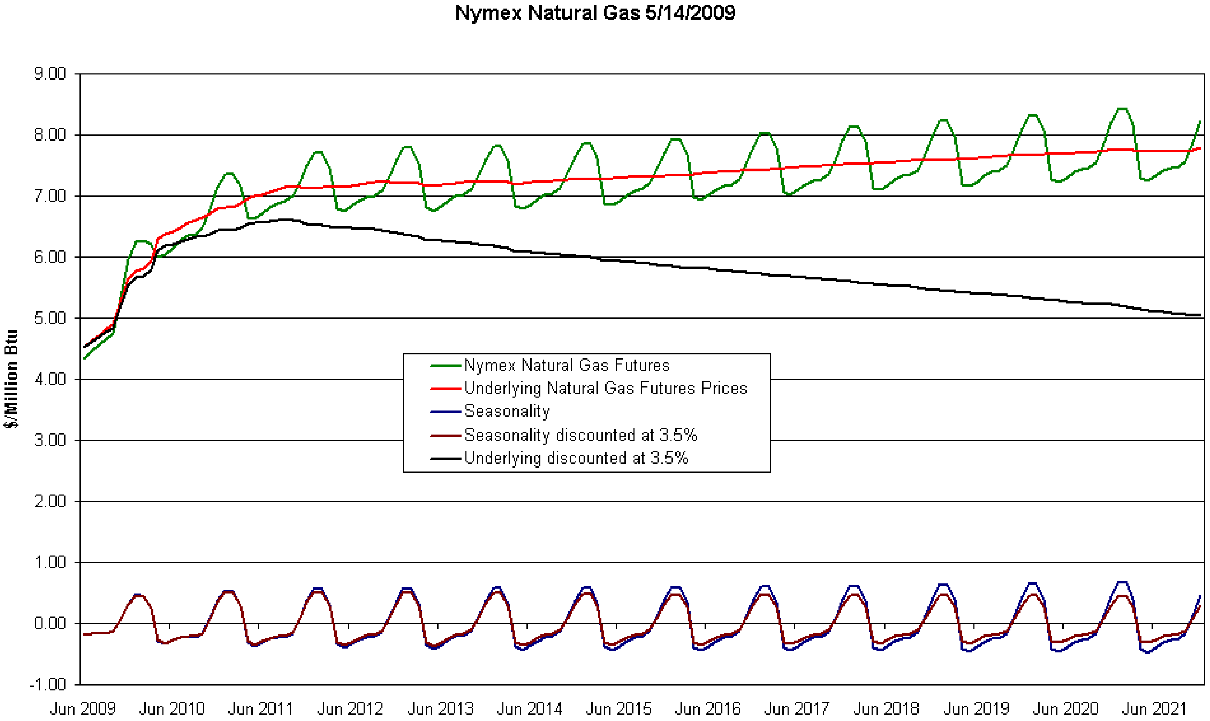
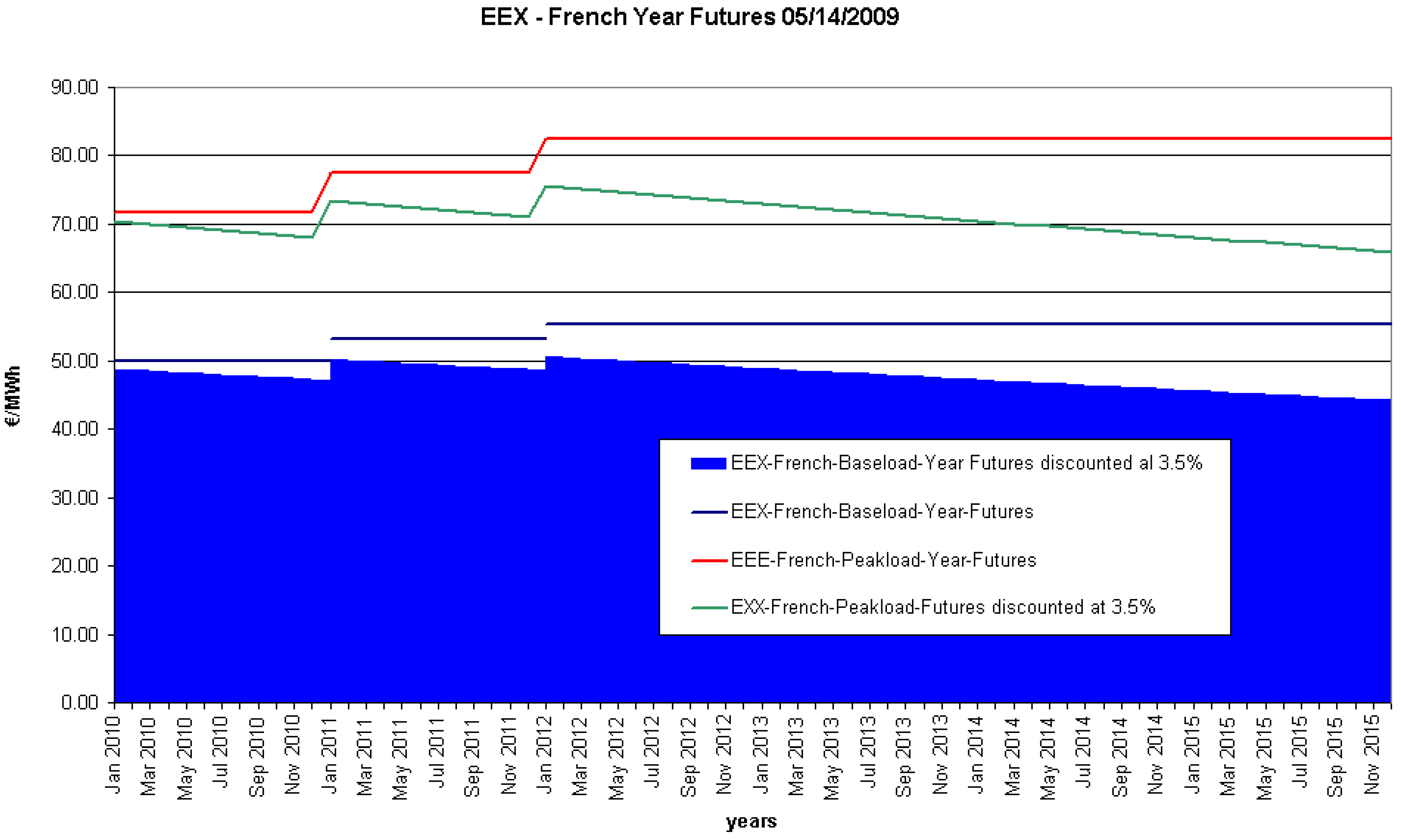
5.1. Seasonality and valuation of annuities

We are going to analyze the relevance of seasonality for different types of models14.
(A) There is a first group of models based on the spot price.
If the model for the futures price F ( S 0 , t ) has been calibrated with a deseasonalised series, seasonality can be imposed by adding a deterministic term f ( t ) . In this way, for a current spot price S 0 of the commodity, we have that a futures contract with maturity at t has a value f ( t ) + F ( S 0 - f ( 0 ) , t ) , where S 0 - f ( 0 ) is the time-0 deseasonalised value.
If we must compute the value of an annuity we use:
V τ 1 , τ 2 = τ 1 τ 2 e - r t f ( t ) d t + τ 1 τ 2 e - r t F ( S 0 - f ( 0 ) , t ) d t
the second integral is the same as in the former cases, but now applies to the deseasonalised series.
When τ 2 τ 1 and τ 2 - τ 1 equals an integer number of years, the first integral is:
τ 1 τ 2 e - r t f ( t ) d t 0
Usually an integer number of years of useful life is assumed. Anyway, the exact dates τ 1 and τ 2 are uncertain (sometimes the precise month when operations start cannot be learnt in advance). Thus, it is more convenient to abandon this procedure and work directly with the deseasonalised series instead.
(B) A second group of models is based on the natural logarithm of the spot price:
ln S t = g ( t ) + X t
where at the initial time X 0 = ln S 0 - g ( 0 ) . The variable X t stands for the deseasonalised series of the log prices.
The formula for the futures price in this case is:
F ( S 0 , t ) = e g ( t ) F ( e X 0 , t )
The integral can be solved by numerical methods:
V τ 1 , τ 2 = τ 1 τ 2 e - r t + g ( t ) F ( e X 0 , t ) d t
As an example, consider the prices on the NYMEX futures market for natural gas on 5/14/2009; they are plotted in Figure 1. From both discounted and un-discounted seasonality patterns it can easily be deduced that, for an integer number n of years, n τ 1 τ 1 + n e - r t f ( t ) d t 0 without any need for an explicit solution to f ( t ) . Even with a non-integer number of years we have:
τ 1 τ 2 e - r t f ( t ) d t τ 1 τ 2 e - r t F ( S 0 - f ( 0 ) , t ) d t
For the data in Figure 1, it is possible to get the un-discounted value of seasonality as the area between the blue curve and the horizontal axis (with positive or negative signs). The discounted value (at a 3.5% rate) of seasonality (which also resembles a smoothed sinusoid) is given by the area between the brown curve and the horizontal axis. We can get these values for a set of whole years from June-2009 to June-2021, yielding:
Figure 1. Futures prices of natural gas on NYMEX 05/14/2009.
Energies 02 00738 g001
Table 1. Seasonal component June-2009 to June-2021 ($/million Btu year).
without discountingdiscounted at 3 . 5 %
0.0210.008
In Figure 1 the value of an annuity from time τ 1 to τ 2 will be given by the area below the underlying (i.e., deseasonalised) black curve discounted at the rate 3.5% between dates τ 1 and τ 2 . This figure also shows that it is possible to derive graphically a rather accurate value of an annuity between τ 1 and τ 2 without the need to estimate the model’s parameters. However, estimation of the parameters would be essential in the valuation of options.
As can be seen in the figure, there are prices over 12.5 years, yet the investments we want to value have a very long useful life in addition to a construction time. For example, in the case of a NGCC power plant, construction takes 2.5 years and the plant’s life stretches over 25 years. In such cases, estimation of the parameters in the futures market model and their application in the formula for the futures price with a longer maturity t could be used for valuing investments.

5.2. Jumps and valuation of annuities

Certain energy products may show jumps in their prices and their spot markets are characterized by great volatility. See, for instance, the French electricity market Powernext (Paris). The base load15 prices from 11/27/2001 to 05/17/2009 are displayed in Figure 2. The peak load prices are plotted in Figure 3; they show a higher volatility.
In order to value derivative assets on a spot electricity market it is necessary to develop and calibrate a complex model like the following16:
d S t = π ( S t , t ) d t + σ S t d W t + S t U t d N t
where π ( S t , t ) is the drift term (which must show seasonality and mean reversion), N t is a Poisson process with a given intensity of jumps, and U t is a random variable that measures the size of the jump.
As a consequence, the formula for a futures contract on a given day F ( S 0 , t ) would be complex and dependent on the former parameters. Nonetheless, it is customary in electricity markets that futures contracts refer to delivery of one MWh hourly over a given period of time, e.g., one year. Therefore, its value F ( S 0 , τ 1 , τ 2 ) for the period between τ 1 and τ 2 would be:
F ( S 0 , τ 1 , τ 2 ) = 1 τ 2 - τ 1 τ 1 τ 2 F ( S 0 , t ) d t
If τ 2 - τ 1 = 1 year, then this reduces to:
F ( S 0 , τ 1 , τ 1 + 1 ) = τ 1 τ 1 + 1 F ( S 0 , t ) d t
Since this formula is an average of values, it can be expected that futures contracts with delivery time of one year do not show jumps, and that revenues at times of jumps in electricity prices are included in this average value; indeed this can be observed in Figure 4 from the European Energy Exchange. Noting that time is typically measured in years, the blue area in this figure shows the current price for delivery of one MWh over six years starting in early 2010. Figure 4 allows to value the profits from producing and selling (or costs to consuming) electricity while taking into account the market price of risk for electricity.
Figure 2. Base load electricity prices on Powernext (France).
Energies 02 00738 g002
If we have the price of yearly futures contracts F ( S 0 , τ 1 + n , τ 1 + ( n + 1 ) ) , with n = 0 , 1 , 2 , . . , m - 1 17, the value of an annuity between τ 1 and τ 2 can be computed as18:
n = 0 n = m - 1 τ 1 + n τ 1 + ( n + 1 ) e - r t F ( S 0 , τ 1 + n , τ 1 + ( n + 1 ) ) d t
Another way of testing the non-existence of jumps in the yearly averages is computing the averages of the spot prices, which appear in Table 2, for the same data as in Figure 2 and Figure 3.

5.3. Stochastic volatility and valuation of annuities
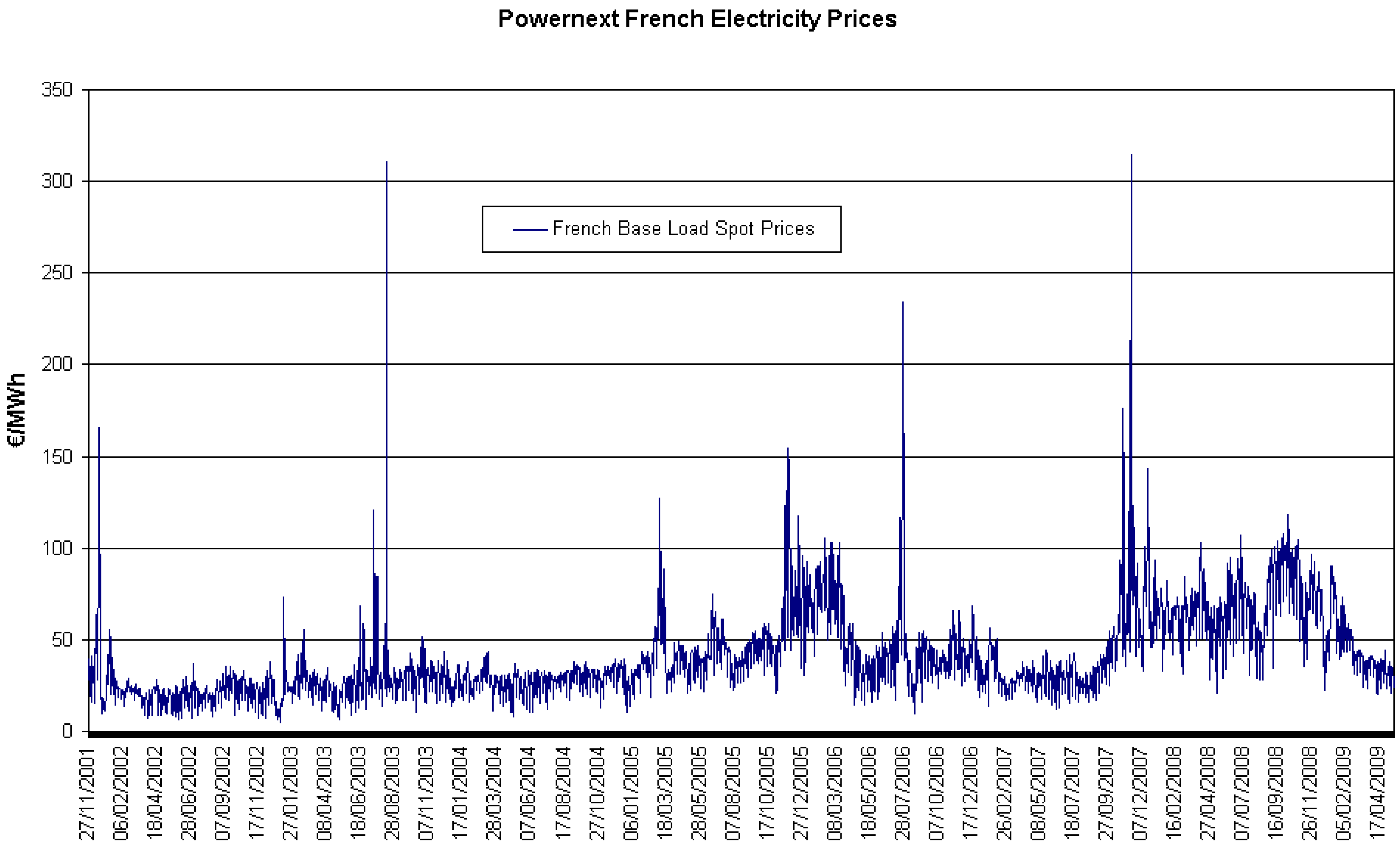
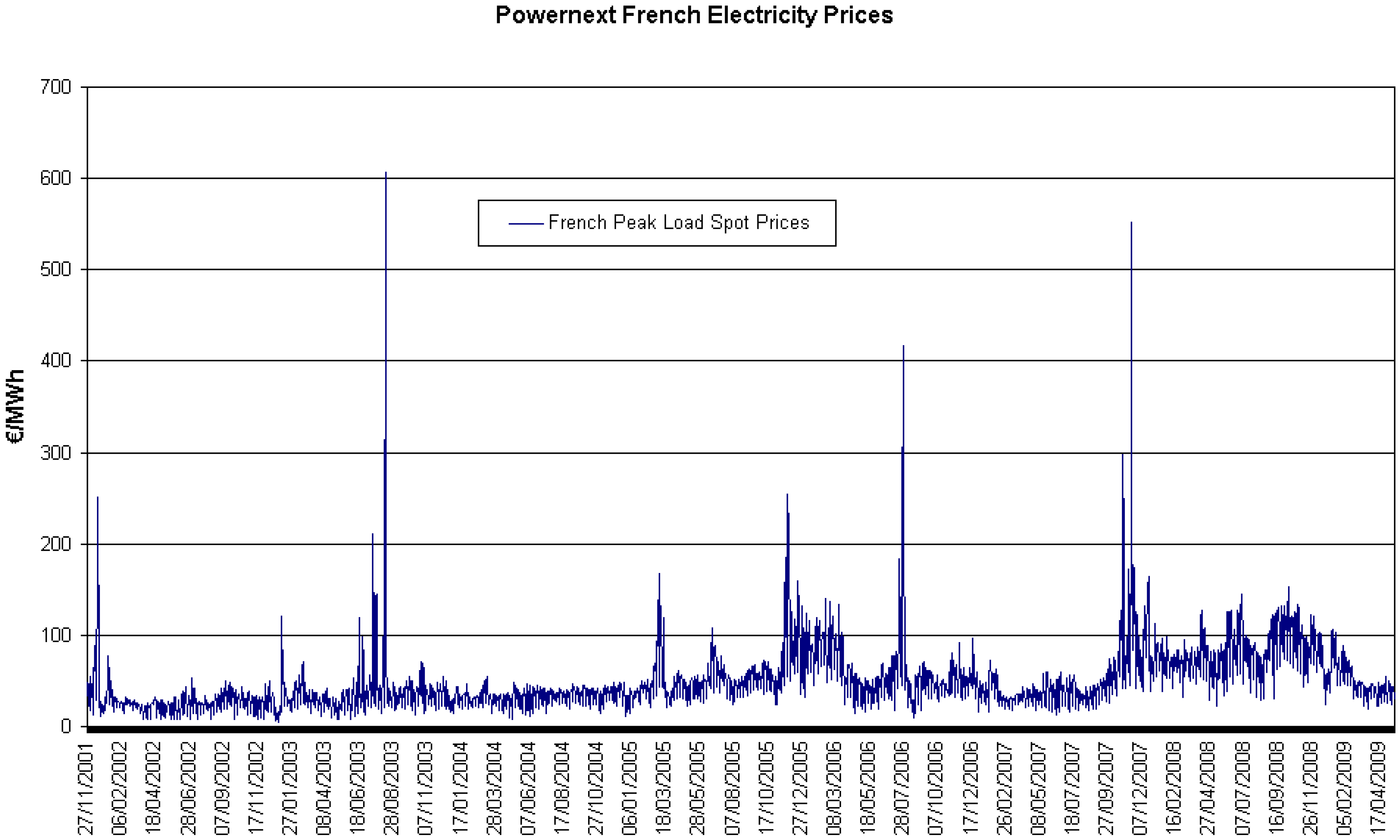
To show the potential impact of volatility on valuation we choose a simple model where the price S t follows a GBM and the variance follows a mean-reverting process:
d S t = α S t d t + σ t S t d W t
d ( σ t 2 ) = a ( σ m 2 - σ t 2 ) d t + b σ t 2 d W t
where σ m 2 is the expected variance in the long term, a denotes the speed of reversion and b stands for the volatility of the variance.
Table 2. Average prices of French electricity.
yearBasePeak
200221.1925.82
200329.2237.82
200428.1333.71
200546.6756.88
200649.2961.07
200740.8751.49
200869.1582.91
Figure 3. Peak load electricity prices on Powernext (France).
Energies 02 00738 g003
The variance σ t 2 has a conditional mean:
E ( σ t 2 ) = σ 0 2 e - a t + σ m 2 ( 1 - e - a t )
This means that, for high values of a, the variance will quickly return to its equilibrium value; also E ( σ 2 ) = σ m 2 . Intuitively, for high values of a as compared to volatility, using σ m in Equation (10) would be a good approximation for valuing long-term annuities, thus neglecting its behavior in the short term. Valuation should be undertaken in a risk-neutral context, so the risk premia should be deducted:
d S t = ( α - λ ) S t d t + σ t S t d W t
d ( σ t 2 ) = a ( σ m * 2 - σ t 2 ) d t + b σ t 2 d W t
where σ m * 2 is the long-term value of the variance under risk neutrality.
Figure 4. Futures prices of French electricity on EEX (Germany).
Energies 02 00738 g004
Let us analyze the case in which initially S 0 = 100 and σ 0 = σ m * , with α - λ = 0 . 03 and different values of σ m * , a and b. We are going to derive the present value of an annuity over 20 years by Monte Carlo (MC) simulation. Namely we run 40,000 simulations over 20 years with 60 steps per year, and r = 0 . 035 . The results are shown in Table 3.
According to Equation 9 V 0 , 20 = 1 , 903 . 25 , which is very close to the values derived by MC simulation. If volatility is actually stochastic but reverts to an equilibrium value, in most of the cases involving projects with constant energy flows it can be enough to use a model devoid of this feature. Note, though, that it may well be very relevant in another type of operations in the short run.
Table 3. Value of V 0 , 20 under Stochastic Volatility.
ab σ m * = 0 . 20 σ m * = 0 . 40
0.50.51,9041,900
0.51.01,9041,921
1.00.51,9041,899
1.01.01,9041,905

5.4. Stochastic dynamics in the long-term level and valuation of annuities

The equilibrium price level in the long run S m can change over time in a deterministic or stochastic pattern. For instance, it can be increasing with the inflation rate. Let us consider this model:
d S t = k ( L t - S t ) d t + σ S S t d W t S
d L t = μ ( L m - L t ) d t + ξ L t d W t L
where S t denotes the time-t price, and L t is the equilibrium price level, which behaves according to Equation 14. k stands for the speed of reversion of price towards its “normal” level; we can compute it as k = ln 2 t 1 / 2 , where t 1 / 2 is the expected half-life, that is, the time for the gap between S t and L t to halve. σ S is the instantaneous volatility; μ is the speed of reversion of L t towards its longer-term equilibrium value L m ; ξ denotes the instantaneous volatility of the equilibrium price. d W t S and d W t L are increments to standard Wiener processes. These increments are assumed to be normally distributed with mean zero and variance d t . We further assume that d W t S d W t L = ρ d t .
This model has some convenient implications: there is no chance for S t or L t to take on negative values; it allows the existence of an equilibrium level, but it is not constant; the expected value of the long-term equilibrium price remains finite, L m 19. Further, the stochastic process for commodity price is similar to the model in Pilipović [19]; yet they differ in that Equation 14 above is of the IGBM type, as opposed to the standard GBM in Pilipović. This kind of model seems preferable if the equilibrium price in the longer term is jointly determined by production cost and demand level. The model allows for market gyrations and wild swings in prices depending on parameter values. Admittedly, it does not account for discontinuous events that give rise to jumps. However, it also allows, as a particular case, that Equations 13 and 14 adopt a GBM format, again depending on the values of the parameters. Last, consistent with futures markets, volatilities do not grow without bound as t ; instead, they approach a finite value if reversion speed is high enough in relation to volatility.
It can be shown that the expected value of the price is:
E ( S t ) = L m - k ( L 0 - L m ) μ - k e - μ t + S 0 - L m + k ( L 0 - L m ) μ - k e - k t
Denoting the risk premia by λ S S ^ t and λ l L ^ t , the dynamics in a risk-neutral setting would be:
d S ^ t = [ k ( L ^ t - S ^ t ) - λ S S ^ t ] d t + σ S S ^ t d W t S
d L ^ t = [ μ ( L m - L ^ t ) - λ l L ^ t ] d t + ξ L ^ t d W t L
In this context, the expected value of the price may be shown to be:
F ( S 0 , L 0 , t ) = E ( S ^ t ) = μ k L m ( μ + λ l ) ( k + λ S ) 1 - e - ( k + λ S ) t + μ k L m ( μ + λ l ) ( μ + λ l - k - λ S ) - k L 0 ( μ + λ l - k - λ S ) · e - ( μ + λ l ) t - e - ( k + λ S ) t + S 0 e - ( k + λ S ) t
The expected value E ( S ^ t ) equals the estimated futures price F ^ t for maturity t. For an arbitrarily long maturity, the estimate for the futures price is:
F ^ = μ k L m ( μ + λ l ) ( k + λ S )
In this case, the value of an annuity is:
V τ 1 , τ 2 = μ k L m r ( μ + λ l ) ( k + λ S ) ( e - r τ 1 - e - r τ 2 )
+ μ k L m ( μ + λ l ) ( k g + λ g ) ( k + λ S + r ) ( e - ( k + λ S + r ) τ 2 - e - ( k + λ S + r ) τ 1 )
+ k L 0 ( μ + λ l - k - λ S ) ( μ + r + λ l ) ( e - ( μ + λ l + r ) τ 2 - e - ( μ + λ l + r ) τ 1 )
+ k L 0 ( μ + λ l - k - λ S ) ( k + r + λ S ) ( e - ( k + λ S + r ) τ 1 - e - ( k + λ S + r ) τ 2 )
+ μ k L m ( μ + λ l ) ( μ + λ l - k - λ S ) ( μ + r + λ l ) ( e - ( μ + λ l + r ) τ 1 - e - ( μ + λ l + r ) τ 2 )
+ μ k L m ( μ + λ l ) ( μ + λ l - k - λ S ) ( k + r + λ S ) ( e - ( k + λ S + r ) τ 2 - e - ( k + λ S + r ) τ 1 )
+ S 0 k + r + λ S ( e - ( k + λ S + r ) τ 1 - e - ( k + λ S + r ) τ 2 )
The value of L m in relation to L 0 has a great impact on the value of the annuity.
If the long-run equilibrium price follows a GBM, L m = 0 and μ = - φ , then:
V τ 1 , τ 2 = k L 0 ( λ l - φ - k - λ S ) ( r + λ l - φ ) ( e - ( λ l - φ + r ) τ 2 - e - ( λ l - φ + r ) τ 1 )
+ k L 0 ( λ l - φ - k - λ S ) ( k + r + λ S ) ( e - ( k + λ S + r ) τ 1 - e - ( k + λ S + r ) τ 2 )
+ S 0 k + r + λ S ( e - ( k + λ S + r ) τ 1 - e - ( k + λ S + r ) τ 2 )
In this case, the results are affected by the drift rate φ of the GBM and the risk premium λ l . A positive drift leads to a higher annuity value, while a positive risk premium reduces the value of the annuity.
If the long-run growth path is only deterministic, i.e., ξ = 0 , λ l = 0 , and L m = 0 , μ = - φ , then:
V τ 1 , τ 2 = k L 0 ( φ + k + λ S ) ( r - φ ) ( e - ( r - φ ) τ 1 - e - ( r - φ ) τ 2 ) + S 0 - k L 0 ( φ + k + λ S ) k + r + λ S ( e - ( k + λ S + r ) τ 1 - e - ( k + λ S + r ) τ 2 )
this is a generalization to Equation 8, but in this case a higher annuity value results if φ > 0 . And a high enough value of k leads to:
V τ 1 , τ 2 L 0 ( r - φ ) ( e - ( r - φ ) τ 1 - e - ( r - φ ) τ 2 )
This figure is also higher than that computed from Equation 9 when φ > 0 . The opposite would happen if φ < 0 , which could occur in some instances.
The above computations show the importance of long-term dynamics. Considering it can change annuity valuation both at present and in the future. It can be later used in a numerical application, like a binomial lattice or a Monte Carlo simulation.

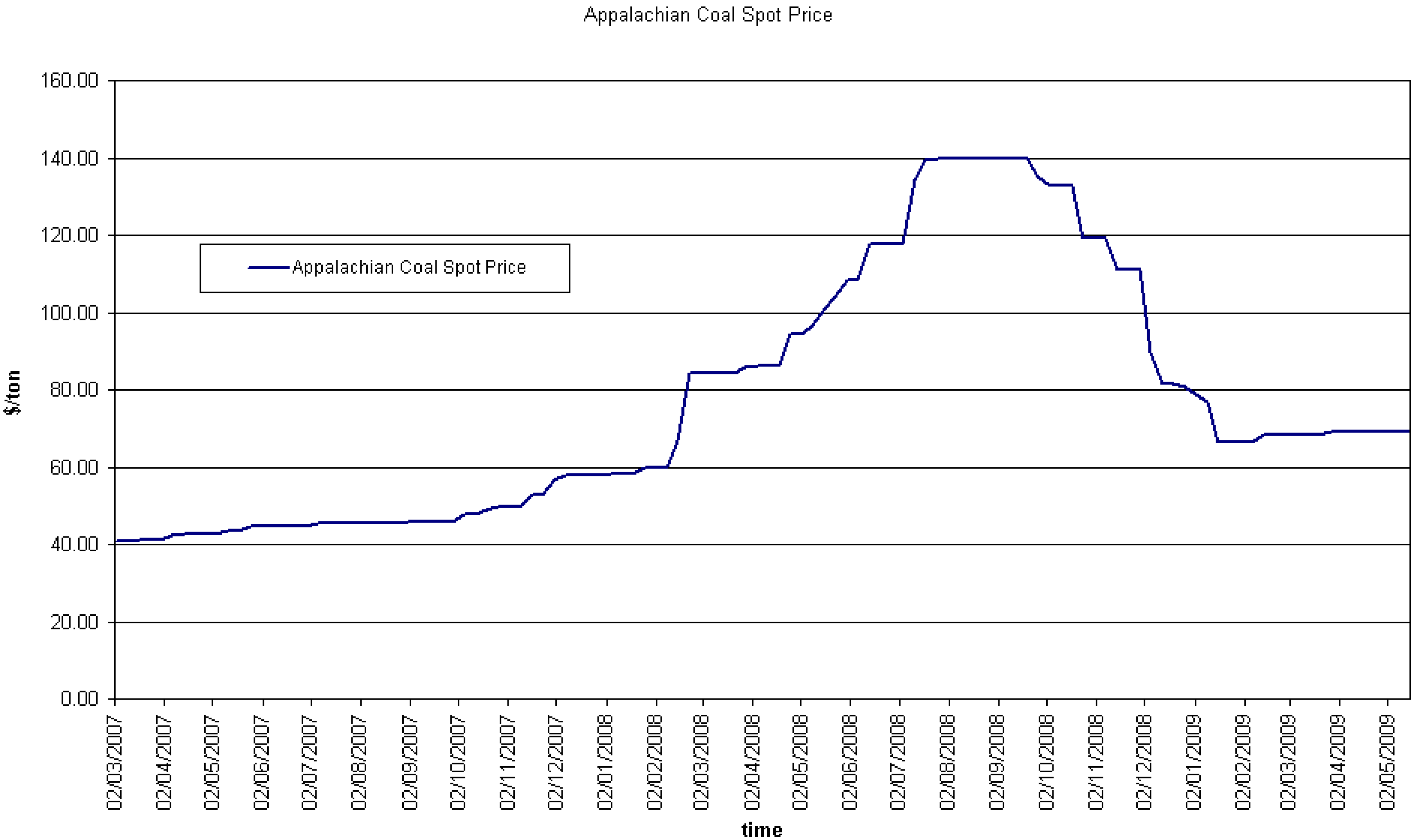
6. Case Study: Improvement in Coal Consumption

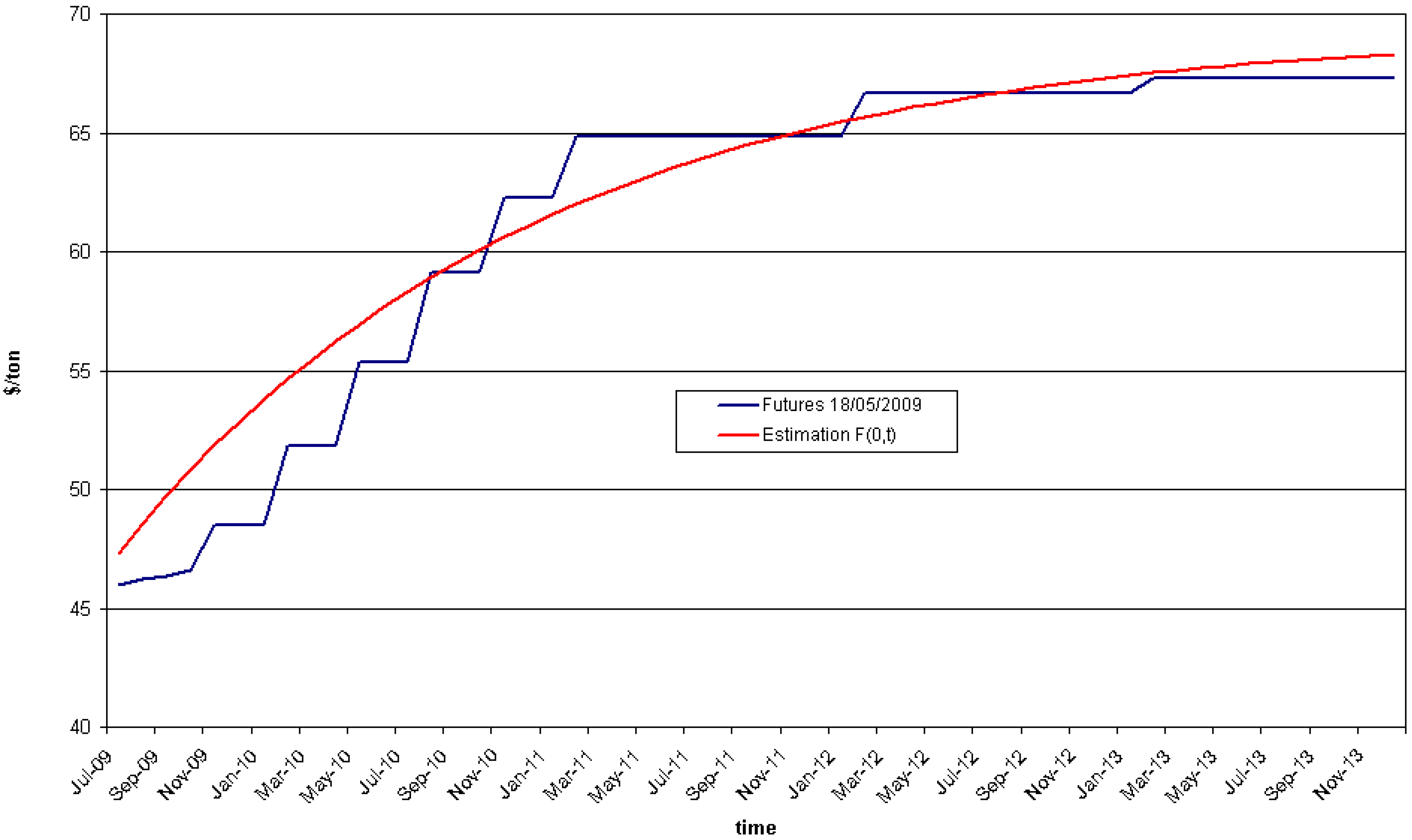
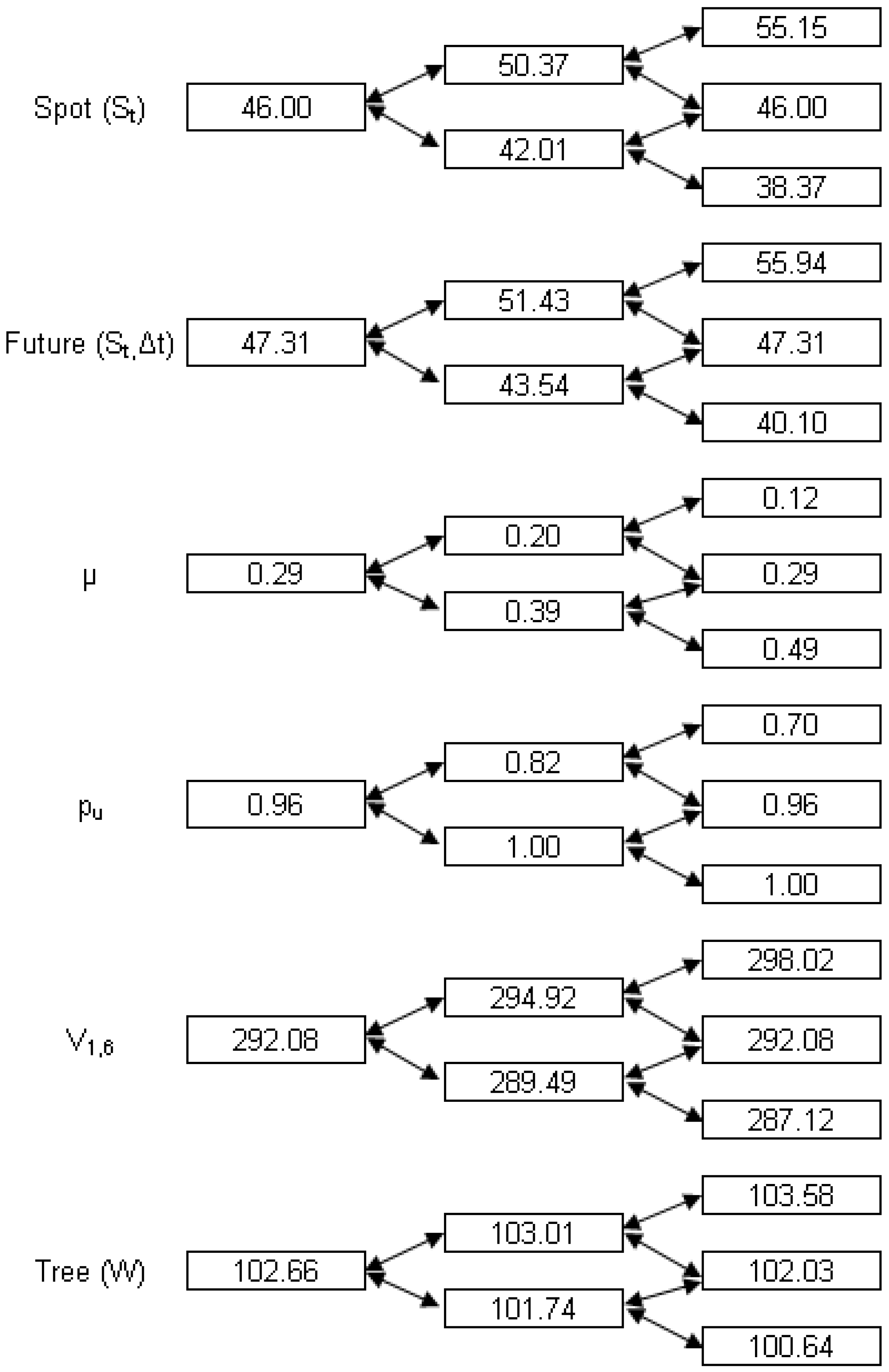
6.1. Case study under uncertainty

As an illustration of this paper, let us analyze the case of an efficiency improvement in the consumption of coal. In particular, every year (over a given time horizon) the firm can avoid burning a ton of Appalachian Coal in exchange for an initial investment I per unit of coal saved. The investment would allow a saving in coal over five years, starting in τ 1 = 1 until τ 2 = 6 , where the dates τ 1 and τ 2 are measured on the basis of the time at which the decision to invest is made. Assume also that this option to invest is only available for one year; it is possible to choose the time to invest. The riskless interest rate is r = 0 . 035 . The value I is the present value, discounted at the risk-free rate, of all the expenses that are needed to realize this saving20. The sum saved is further assumed to be the spot price of Appalachian Coal, so the total savings over five years can be valued by discounting the prices on the NYMEX futures market.
The prices in Figure 5 show some movements in the last months. This implies a higher volatility, the size of which we are going to estimate. As explained in Wilmott [5], when Δ t is small, volatility can be computed as:
σ = 1 ( N - 1 ) Δ t i = 1 N ( ln S t i - ln S t i - Δ t ) 2
From the series of weekly spot prices between 3/02/07 and 5/15/09 we get an estimate of volatility σ = 0 . 3142 .
Figure 5. Spot price of Appalachian coal on NYMEX.
Energies 02 00738 g005
We are going to undertake an estimation with a one-factor model. Mere observation of actual prices in Figure 6 suggests that the GBM would not be a suitable model, since in this case the futures equation would be F ( S 0 , t ) = S 0 e ( r - δ ) t ; this would lead to a growing increase (in absolute value) between equidistant futures prices if r - δ > 0 , which is not the case in Figure 6.
Therefore, next we use a model for the futures market of the IGBM type which is given by Equation 6:
F ( 0 , t ) = k S m k + λ [ 1 - e - ( k + λ ) t ] + S 0 e - ( k + λ ) t
We calibrate the model by comparing the theoretical prices with the actual prices on 5/18/09 so as the sum of squared errors to be minimum. From the above equation we deduce that we can only estimate U 1 k S m / ( k + λ ) and U 2 k + λ ; actually we do not need more parameters to value the option to invest21. We get U 1 = 69 . 3715 and U 2 = 0 . 6905 . We have neither computed the equilibrium value S m , nor the speed of reversion k, nor the risk premium λ. Yet with the values of U 1 and U 2 we are able to value a stochastic income at the current time following Equation (8), now stated in terms of S 0 , U 1 and U 2 :
V 1 , 6 ( S 0 , U 1 , U 2 ) = U 1 ( e - r - e - 6 r ) r + S 0 - U 1 r + U 2 ( e - ( r + U 2 ) - e - 6 ( r + U 2 ) )
The value U 1 = 69 . 3715 is consistent with the asymptotic behavior of the futures curve in Figure 6. On the other hand, from U 2 k + λ = 0 . 6905 we deduce that t 1 / 2 * = ln 2 / ( k + λ ) = 1 . 0038 ; hence, it will take a year to reach the mid point between the spot price and the long-term equilibrium price. The latter turns out to be 57 . 69 . It can be seen in Figure 6 that this value is consistent with the graph displaying the futures curve. The last price available corresponds to a 4.5 years maturity, at 67.28 $/ton, while the futures curve estimated for this maturity is 68.33 $/ton. Since U 1 = 69 . 3715 $/ton any value derived from extending the curve for t > 4 . 5 will fall between 68.33 $/ton and 69.37 $/ton, which amounts to a very narrow spread and would be consistent with Figure 6.
Figure 6. Futures prices of Appalachian coal on NYMEX.
Energies 02 00738 g006
Provided the parameters U 1 and U 2 are stable over time, Equation 23 allows to compute the value of this annuity if we decide to invest at a particular node of the binomial lattice or a particular point in a simulation path. It would be enough to replace S 0 with the value S t derived at that time by computing V τ 1 , τ 2 ( S t , U 1 , U 2 ) 22.
We develop the case study with a (one-dimensional) binomial lattice which supports a stochastic process with mean reversion. The initial spot price is 46.00 $/ton. Equation 5 showed the behavior of the commodity in the risk-neutral setting under the model adopted:
d S ^ t = [ k ( S m - S ^ t ) - λ S ^ t ] d t + σ S ^ t d Z t
This can also be written as:
d S ^ = ( k ( S m - S ^ ) S ^ - λ ) S ^ d t + σ S ^ d Z
We use the following logarithmic transformation of the price: X ln S ^ . The resulting derivatives are X s = 1 / S ^ , X s s = - 1 / S ^ 2 , X t = 0 , and by Ito’s Lemma:
d X = ( k ( S m - S ^ ) S ^ - λ - 1 2 σ 2 ) d t + σ d Z = μ ^ d t + σ d Z
where μ ^ 1 S ^ ( k S m - ( k + λ ) S ^ ) - 1 2 σ 2 depends at each moment on the current asset value S ^ ; this implies that the risk-neutral probabilities on the binomial lattice will not be constant.
The time horizon T is subdivided in n steps, each of size Δ t = T / n . Starting from an initial value S 0 , at time i, after j positive increments, the value of the commodity is given by S 0 u j d i - j , where d = 1 / u .
When Δ t is very small, Equation 6 becomes:
F ( 0 , Δ t ) = k S m k + λ [ 1 - e - ( k + λ ) Δ t ] + S 0 e - ( k + λ ) Δ t S 0 + k S m Δ t - S 0 ( k + λ ) Δ t
Therefore:
F ( 0 , Δ t ) - S 0 [ k S m - S 0 ( k + λ ) ] Δ t
Hence:
μ ^ F ( S ^ , Δ t ) - S ^ S ^ Δ t - 1 2 σ 2
Following Euler-Maruyama’s discretization, the probabilities of upward and downward movements must satisfy three conditions:
  • (a) p u + p d = 1 .
  • (b) E ( Δ X ) = p u Δ X - p d Δ X = F ( S ^ , Δ t ) - S ^ S ^ Δ t - 1 2 σ 2 Δ t = μ ^ Δ t . The aim is to equate the first moment of the binomial lattice ( p u Δ X - p d Δ X ) to the first moment of the risk-neutral underlying variable ( μ ^ Δ t ).
  • (c) E ( Δ X 2 ) = p u Δ X 2 + p d Δ X 2 = σ 2 Δ t + μ ^ 2 ( Δ t ) 2 . In this case the equality refers to the second moments. For small values of Δ t , we have E ( Δ X 2 ) σ 2 Δ t .
From (a) and (b) we obtain the probabilities, which can be different at each point of the lattice (because μ ^ depends on S ^ , which may vary from node to node):
p u = 1 2 + μ ^ Δ t 2 Δ X
We must be sure that probabilities do not take on negative values.
From (c) there results Δ X = σ Δ t ; therefore, u = e σ Δ t , which guarantees that the branches of the lattice recombine. The probability of an upward movement at point ( i , j ) is:
p u ( i , j ) = 1 2 + μ ^ ( i , j ) Δ t 2 σ
where:
μ ^ ( i , j ) F ( S ^ ( i , j ) , Δ t ) - S ^ ( i , j ) S ^ ( i , j ) Δ t - 1 2 σ 2
thus, μ ^ ( i , j ) depends on the value reached by the price S ^ ( i , j ) .
We divide the year in which the option to invest can be exercised into twelve periods Δ t = 1 / 12 , which implies Δ X = σ 1 / 12 = 0 . 0907 and u = 1 . 0949 . Initially, F ( 46 . 00 , 1 / 12 ) = 47 . 3069 $/ton. In this way μ ^ ( 0 , 0 ) = 0 . 2916 and p u ( 0 , 0 ) = 0 . 9640 . Since initially X 0 = ln 46 = 3 . 8286 , with probability p u ( 0 , 0 ) = 0 . 9640 it will move upwards to X + X 0 + Δ X = 3 . 9193 , and with probability p d ( 0 , 0 ) = 0 . 0360 it will move downwards to X - X 0 - Δ X = 3 . 7379 . Therefore, in case of going up S ^ ( 1 , 1 ) = S 0 e Δ X = 50 . 37 , while in case of going down S ^ ( 1 , 1 ) = S 0 e - Δ X = 42 . 01 . Thus, at time i after j upward movements we have S ^ ( i , j ) = S 0 e j Δ X - ( i - j ) Δ X .
At the initial moment V 1 , 6 ( 46 . 00 , U 1 , U 2 ) = 292 . 08 $. The value V 1 , 6 ( S 0 , U 1 , U 2 ) is relatively sensitive to changes in S 0 as Table 4 shows.
Table 4. Sensitivity analysis.
S 0 V 1 , 6 ( S 0 , U 1 , U 2 )
40.00288.18
46.00292.08
50.00294.68
55.00297.92
57.69299.67
60.00301.17
Initially we have computed V 1 , 6 ( 46 . 00 , U 1 , U 2 ) = 292 . 08 $. ¿From observation of Equation 23 we deduce that there is a first term related to the contribution of the equilibrium value which adds 307 . 26 $, and a second term related to the difference between the spot price and the equilibrium price in the futures market which subtracts 15 . 18 $. They both give rise to the net result above.
The binomial lattice is solved backwards in the following way. At the final moment, there is only the option either to invest or not to invest. The choice depends on the project value:
W = M a x ( V 1 , 6 ( S 1 , U 1 , U 2 ) - I , 0 )
At earlier times we choose the best of the two alternatives, namely to invest or to continue waiting:
W = M a x ( V 1 , 6 ( S t , U 1 , U 2 ) - I ; e - r Δ t [ p u W + + ( 1 - p u ) W - ] )
Figure 7 shows the first two steps of the binomial lattice and the results of the ensuing computations.
Iterating this process a value of the lattice at time 0, W 0 , will result. This amount is compared with V 1 , 6 ( S 0 , U 1 , U 2 ) - I . If they are equal it will be optimal to invest at the initial moment; instead, if W 0 > V 1 , 6 ( S 0 , U 1 , U 2 ) - I it will be optimal to wait. By changing the value of I until W 0 and V 1 , 6 ( S 0 , U 1 , U 2 ) - I become equal we compute the critical (or "trigger") value I * to invest at time 0 under current conditions.
In our example there is no positive value of I * for which W 0 = V 1 , 6 ( S 0 , U 1 , U 2 ) - I * . This is because, presumably, according to the prices in futures markets V 1 , 6 ( S 1 , U 1 , U 2 ) is going to be much bigger on average then V 1 , 6 ( S 0 , U 1 , U 2 ) even after adjusting for the effect of the riskless rate r, so it is optimal to wait. With an initial price S 0 = 46 . 00 and an investment outlay I = 200 we get W 0 = 102 . 66 as opposed to a net present value given by N P V = V 1 , 6 ( 46 . 00 , U 1 , U 2 ) - I = 92 . 08 . These results are the consequence of the parameter values, but they are mainly influenced by uncertainty and market contango.
Figure 7. Computation by a binomial lattice.
Energies 02 00738 g007
The situation would change substantially if the spot price suddenly increased to S 0 = 70 . 00 while keeping the same values U 1 and U 2 . In this case W 0 = 108 . 00 with I = 200 and V 1 , 6 ( 70 . 00 , U 1 , U 2 ) - I = 107 . 67 ; therefore, it would be optimal to invest immediately. It is also possible to derive a critical value I * = 168 . 74 below which it would be optimal to invest; for this threshold value W 0 = V 1 , 6 ( 70 . 00 , U 1 , U 2 ) - I * = 138 . 93 .

6.2. Case study: NPV and IRR

Now we are going to assess the same case using the NPV and the IRR. To that end in the first case we will need a discount rate, and in both cases we will need to estimate the expected cash flows. The computations are made disregarding futures market prices. We are going to see for what parameter values we reach an equivalent result.
Let us assume that the analyst, without using market data, thinks that starting from the current price of S 0 = 46 . 00 $ / t o n it can grow in the physical world at a rate φ and that she/he must discount the investments by adding a risk premium λ to r. The analyst will value the investment according to:
N P V = V τ 1 , τ 2 - I = S 0 ( r + λ - φ ) ( e - ( r + λ - φ ) τ 1 - e - ( r + λ - φ ) τ 2 ) - I
where the disbursement I takes place at the initial moment. In fact, in this approach mean reversion in prices would be ignored.
Actually, to make the valuation, according to the former equation, the analyst would only need to choose a value for r + λ - φ . See Table 5.
Table 5. Sensitivity of V τ 1 , τ 2 .
r + λ - φ V τ 1 , τ 2
-0.10329.80
-0.067292.08
-0.05274.70
0.00230.00
0.05193.58
0.10163.77
In order to derive an identical value to that resulting from futures prices it would be necessary a value r + λ - φ = - 0 . 067 . Given that we are assuming a riskless rate r = 0 . 035 it should be φ - λ = 0 . 102 , which would be valid for several combinations. For example, assuming a real expected growth in prices φ = 0 . 15 , the risk premium would be λ = 0 . 048 , so the cash flows would be discounted at a rate r + λ = 0 . 083 . It seems very unlikely that using firm-level discount rates (instead of project-specific rates), adjusted by risk, we get a result consistent with the market.
On the other hand, with the NPV we are not valuing the optionality. For instance, if we have I = 150 we will accept the investment project right now for a wide range of values of r + λ - φ , which would not be optimal when the option to wait is considered.
In this same case, when I = 150 we can compute the IRR as the value such that
I = S 0 ( I R R - φ ) ( e - ( I R R - φ ) τ 1 - e - ( I R R - φ ) τ 2 )
If we think that φ = 0 . 15 , we will get a value I R R = 0 . 2769 (or 27.69%), which may seem enough to invest in a project, but again we are forgetting the option to wait.

6.3. Case study: σ = 0

When σ = 0 there is no uncertainty and hence no risk, so it must be λ = 0 . In this case, E 0 ( S t ) = F ( S 0 , t ) . In this situation it is possible to determine the optimal time to invest T * which does not necessarily coincide with the initial time.
In this case U 1 = S m and U 2 = k . The spot price at the optimal investment time T * is given by:
S T * = U 1 + [ S 0 - U 1 ] e - U 2 T *
This way the present value of the investment undertaken at T * is
[ V 1 , 6 ( S T * , U 1 , U 2 ) - I ] e - r T * = [ U 1 ( e - r - e - 6 r ) r + S T * - U 1 r + U 2 ( e - ( r + U 2 ) - e - 6 ( r + U 2 ) ) - I ] e - r T *
= [ U 1 ( e - r - e - 6 r ) r + [ S 0 - U 1 ] e - U 2 * T * r + U 2 ( e - ( r + U 2 ) - e - 6 ( r + U 2 ) ) - I ] e - r T *
where we assume a constant value of I through time.
Differentiating with respect to T * and equating to zero we get:
T * = - 1 U 2 ln r I - U 1 ( e - r - e - 6 r ) ( S 0 - U 1 ) ( e - ( r + U 2 ) - e - 6 ( r + U 2 )
For the values of the case study we can easily get T * = 1 . 0045 . It is slightly longer than a year, which is the term when the opportunity to invest is available. Since the present value of the future investment is increasing until T * = 1 . 0045 , in fact the optimal time to invest will be the final moment T * = 1 . 00 . This case shows that, even without volatility, and therefore without risk, it may be suboptimal to invest at the initial time despite N P V > 0 . Market contango does not promote immediate investments to enhance energy efficiency even if a zero risk premium were assumed (because of a hypothetical absence of volatility).

7. Conclusions

In this paper we have analyzed how to value investments in energy assets that continuously produce and/or consume certain commodities which are traded in futures markets. The existence of ever more liquid futures markets, with contracts with ever longer maturities, makes it possible to value real assets consistently with futures prices.
We have discussed the weaknesses and difficulties of using other alternative approaches such as the NPV when only one rate is used to discount cash flows and both expected flows and risk premia must be estimated. As we have shown, a model which links each cash flow to its market manages to reflect the risks of a project when there are no options, and is the starting point to value different types of options.
We have analyzed several usual procedures to model futures markets. We have also derived the corresponding formula for valuing stochastic incomes using the valuation methods well-known to energy-finance academics. We have seen the reduced impact of short-term phenomena like seasonality, jumps or stochastic volatility, on these long-term valuations. Nonetheless, they would be essential for the valuation of short-term derivatives.
Similarly, we have seen that the long-run equilibrium price in a risk-neutral setting is of paramount importance as an input to the valuation of investments with long lives. We have also analyzed the impact of reversion to the mean on the valuation of cash flows; specifically, a strong reversion entails a lower risk.
Last, we have developed a valuation exercise of improvement in coal consumption to illustrate the above mentioned concepts. The results of the example show the impact of uncertainty and the shape of the futures curve on decision making when there is some option at hand, like the opportunity to delay an investment to improve energy efficiency. In these cases, high uncertainty coupled with market contango can make that, even with a zero cost of the investment in efficiency (it could be subsidized), some investments are not undertaken on sole economic rationality grounds. Even in situations of certainty, it could be optimal to postpone an investment if the market shows contango. Therefore, promotion of investments to enhance efficiency should take into account these issues to be more effective since, unless these investments are undertaken, higher CO 2 emissions will be poured to the atmosphere. Last, we have seen that it is highly unlikely that a valuation based only on the NPV or the IRR provides results consistent with the market if market information is neglected; this holds irrespective of whether there are options or not. Similarly, valuations should take into account the information embedded in the futures curve, i.e., if the market shows backwardation or contango, to avoid misleading values. Clearly there is a need for a deeper analysis when the long-term equilibrium value is not constant.

Acknowledgements

I thank José M. Chamorro (University of the Basque Country) for his suggestions on a former version of this paper. I also thank three anonymous reviewers for their contributions and remarks.

References

  1. McCardell, S.B. Life Cycle Costing: Energy Projects. In Encyclopedia of Energy Engineering and Technology; Capehart, B.L., Ed.; CRC Press: Gainesville, Florida, USA, 2007; pp. 967–976. [Google Scholar]
  2. Bhattacharjee, U. Life Cycle Costing: Electric Power Projects. In Encyclopedia of Energy Engineering and Technology; Capehart, B.L., Ed.; CRC Press: Gainesville, Florida, USA, 2007; pp. 953–966. [Google Scholar]
  3. McDonald, R.L. Real options and rules of thumb in capital budgeting. In Innovation, Infrastructure and Strategic Options; Brenan, M.J., Trigeorgis, L., Eds.; Oxford University Press: London, UK, 1998. [Google Scholar]
  4. Graham, J.R.; Harvey, C.R. The theory and practice of corporate finance: evidence from the field. J. Finan. Econ. 2001, 60, 187–243. [Google Scholar] [CrossRef]
  5. Wilmott, P. Paul Wilmott on Quantitative Finance; John Wiley & Sons: West Sussex, UK, 2006. [Google Scholar]
  6. Dixit, A.K.; Pindyck, R.S. Investment under Uncertainty; Princeton University Press: Princeton, NJ, USA, 1994. [Google Scholar]
  7. Trigeorgis, L. Real Options - Managerial Flexibility and Strategy in Resource Allocation; The MIT Press: Cambridge, MA, USA, 1996. [Google Scholar]
  8. Ronn, E.I. Real Options and Energy Management Using Options Methodology to Enhance Capital Budgeting Decision; Risk Books: London, UK, 2002. [Google Scholar]
  9. Rocha, K.; Moreira, A.; Divid, P. Thermopower generation investment in Brazil-economics conditions. Energ. Policy 2004, 32, 91–100. [Google Scholar]
  10. Gollier, C.; Proult, D.; Thais, F.; Walgenwitz, G. Choice of electric power investment under uncertainty: the vaue of modularity. Energ. Econ. 2005, 27, 667–685. [Google Scholar] [CrossRef]
  11. Näsäkkälä, E.; Fleten, S.-E. Flexibility and technology choice in gas-fired power plant investments. Rev. Finan. Econ. 2005, 14, 371–393. [Google Scholar] [CrossRef]
  12. Abadie, L.M.; Chamorro, J.M. Valuing flexibility: The case of an Integrated Gasification Combined Cycle power plant. Energ. Econ. 2008, 30, 1850–1881. [Google Scholar] [CrossRef]
  13. Abadie, L.M.; Chamorro, J.M. Monte Carlo valuation of natural gas investments. Rev. Finan. Econ. 2009, 18, 10–22. [Google Scholar] [CrossRef]
  14. Deng, S.-J. Valuation of investment and oportunity-to-invest in power generation assets with spikes in electricity price. Manage. Finan. 2005, 31, 95–115. [Google Scholar]
  15. Deng, S.-J.; Johnson, B.; Sogomonian, A. Exotic electricity options and the valuations of electricity generation and transmision assets. Decis. Support Syst. 2001, 30, 383–392. [Google Scholar] [CrossRef]
  16. Gourieroux, C.; Jasiak, J. Financial Econometrics; Princeton University Press: Princeton, NJ, USA, 2001. [Google Scholar]
  17. Cortazar, G.; Milla, C.; Severino, F. A multicommodity model of futures prices: Using futures prices of one commodity to estimate the stochastic process of another. J. Futures Markets 2008, 28, 537–560. [Google Scholar] [CrossRef]
  18. Schwartz, E.S. The stochastic behavior of commodity prices: Implications for valuation and hedging. J. Finan. 1997, 52, 923–973. [Google Scholar] [CrossRef]
  19. Pilipović, D. Energy Risk; McGraw-Hill: New York, NY, USA, 1997. [Google Scholar]
  20. Dean, J.W. Investment Analysis Techniques. In Encyclopedia of Energy Engineering and Technology; Capehart, B.L., Ed.; CRC Press: Gainesville, FL, USA, 2007; pp. 930–936. [Google Scholar]
  21. Salahor, G. Implications of output price risk and operating leverage for the valuations of petroleum development projects. The Energy Journal 1998, 19, 13–46. [Google Scholar] [CrossRef]
  22. Laughton, D.G.; Sagi, J.S.; Samis, M.R. Modern assets pricing and project evaluation in the energy industry. J. Energ. Lit. 2000, 6, 3–46. [Google Scholar]
  23. Lucia, J.J.; Schwartz, E.S. Electricity prices and power derivatives: Evidence from the nordic power exchange. Rev. Derivatives Res. 2002, 5, 5–50. [Google Scholar] [CrossRef]
  24. Geman, H. Commodities and Commodity Derivatives. Modeling and Pricing for Agricultural, Metals and Energy; Wiley Finance: West Sussex, England, 2005. [Google Scholar]
  • Notes

  • 1.Consider, for example, the time to build a nuclear power plant, which has shown a strong volatility in the last years because of risks that sometimes had not been taken into account initially.
  • 2.The NPV and IRR methods are explained in Dean [20]. But, as the author admits (though it is not developed in his paper), the hardest issue to assess is risk. In real applications it must be included in the valuation together with the options embedded in the project. The NPV would be the starting point.
  • 3.The impact of a high discount rate on the valuation of long-term investments is addressed in Salahor [21] and Laughton et al. [22].
  • 4.Though it is possible to compute it if one wants so. See Salahor [21].
  • 5.A method of this type, though with a different approach, is analyzed in Laughton et al. [22].
  • 6.The value r f is the riskless interest rate on a 365-days basis; it is slightly different from the continuous rate r. For a flat zero-coupon curve r = ln ( 1 + r f ) holds, so discounting can be equivalently accomplished either by multiplying by 1 / ( 1 + r f ) t or by e - r t .
  • 7.If construction costs are high and the construction period is several years long then investments will need funding presumably at a high rate. Also, it will take some time until revenues allow to service the debt and pay the principal back.
  • 8.Some additional reasons are: (a) This model satisfies the following condition (which seems reasonable): if the price of one unit of the asset reverts to some mean value, then the price of two units reverts to twice that same mean value. (b) The term σ S t d Z t precludes, almost surely, the possibility of negative values. (c) The expected value in the long run is: E ( S ) = S m ; this is not so in Schwartz [18] model, where E ( S ) = S m ( e - σ 2 4 k ) .
  • 9.If it is specified as a fixed amount independent of S ^ t , the risk premium would only be λ, and the formulas derived would be slightly different.
  • 10.The value of λ can be negative in certain cases.
  • 11.δ reflects the profits enjoyed by the owner of the physical commodity, as opposed to the holder of a futures contract. It is equivalent to the dividends received by the holder of a firm’s stock (as opposed to the holder of a stock option).
  • 12.In case the model for a given commodity is not mean reverting but GBM, the existence of a convenience yield should be considered.
  • 13.Note that under very fast mean reversion the model in the end behaves as if it stayed constant at this equilibrium value.
  • 14.Lucia and Schwartz [23] analyze the different forms of modeling seasonality and develop an estimation for the Nordic Power Exchange.
  • 15.The term “base load” refers to the type of load for the delivery of electricity or the procurement of electricity with a constant output over 24 hours of each day of the delivery period. The term “peak load”, instead, refers to the load type for the delivery or procurement of electricity at a constant load over 12 hours from 08:00 am until 08:00 pm on every working day (Monday to Friday) during a delivery period.
  • 16.See Geman [24], particularly chapter 11, which deals with Spot and Forward Electricity Markets.
  • 17.We consider m years of useful life.
  • 18.For simplicity we assume that τ 2 - τ 1 = m is an integer number of years.
  • 19.In this model E ( L t ) = L m + ( L 0 - L m ) e - μ t , which implies E ( L ) = L m .
  • 20.For a particular number of tons saved per year, the results would be proportional to those in this example.
  • 21.Though in this case the estimation has been done for just one day, it is possible to do it also with the futures prices on several days to test for the stability of the parameters U 1 and U 2 when the initial spot price changes, or even to calibrate a more complex model (this is beyond the scope of this paper).
  • 22.Where τ 1 and τ 2 are measured from time t.

