
Utilisation of Renewable Electricity to Produce Synthetic Methane
Faculty of Chemistry and Chemical Engineering, University of Maribor, Smetanova 17, 2000 Maribor, Slovenia
*
Author to whom correspondence should be addressed.
Energies 2023, 16(19), 6871; https://doi.org/10.3390/en16196871
Submission received: 31 August 2023
/
Revised: 21 September 2023
/
Accepted: 26 September 2023
/
Published: 28 September 2023
(This article belongs to the Special Issue Energy Transition and Environmental Sustainability II)
Abstract
:This study demonstrates the production of synthetic methane or synthetic natural gas via methanation of carbon dioxide (CO2), which could replace natural gas. For the power-to-methane (P2M) process, a simulation of two-stage methanation with simultaneous power generation was carried out in Aspen Plus. The process is based on an assumed production capacity of 1 t/h of synthetic methane and is also capable of simultaneous methanation of CO2 and biogas. The biogas flow rate was estimated from industry data. When co-methanation is carried out, it is possible to produce up to 1.3 t/h of synthetic methane. After the production of synthetic methane, compression of the product was added to the process scheme, followed by dehydration. The dehydration of the synthetic methane was carried out via dynamic simulation in Aspen Adsorption. The steady-state operation was determined. The final dehydrated product contained on average only about 4.85 × 10⁻⁴ mol.% water (H2O) and the methane (CH4) contents were above 97 mol.%, providing a composition suitable for injection into the pipelines of many European countries.
1. Introduction
In recent years, global warming has been one of the major issues facing humanity. According to the Paris Agreement, the rise in global temperatures must be limited to 1.5 °C compared with pre-industrial levels [1]. Decarbonising existing processes and technologies and switching to renewables are key to achieving these goals.
The trend towards increasing the use of renewable sources for electricity generation is evident. Although among renewables, hydropower, at 1.25 TW, represents the largest share of global generation capacity, wind and solar dominate the newly added generation capacity. Together, both technologies contributed 90% of all renewable energy generation capacity added in 2022 [2].
Even though many new wind and solar power plants have been built, there is a new problem arising with renewables. This is the problem of unpredictable supply and demand [3]. During windy or sunny periods, the supply of electricity is high. In cases where demand for energy is low, this can lead to extremely low, or even negative levelised electricity prices on wholesale markets [4].
Excess renewable energy can be stored to solve the problem of the oversupply of electricity [1]. One storage solution is the power-to-gas (P2G) process, where excess electricity is used to produce hydrogen (H2) via water electrolysis. The hydrogen can then be stored, or injected into natural gas pipelines [3].
Hydrogen storage poses several challenges. Because it is the smallest molecule, it diffuses relatively quickly through the storage tanks [5]. It has a very low boiling point (−252.8 °C), which requires cryogenic temperatures for liquefaction [6], and it also has a very low volumetric energy density. According to the ideal gas law, to supply the same amount of energy as 1 mol of methane, hydrogen must be compressed to 3.318 times the storage pressure of methane [7]. Storing in a gas state therefore requires pressures from 350 to 700 bar [6]. The presence of hydrogen in natural gas pipelines also causes the deterioration of the mechanical properties of steel materials, due to a phenomenon called hydrogen embrittlement [5].
Since direct storage of hydrogen is problematic, storage in the form of methane may be more feasible. With hydrogen, methane can be produced by the Sabatier reaction shown in Equation (1). The produced methane can be referred to as synthetic methane, or synthetic natural gas. The production process can be referred as power-to-methane (P2M) [1]. Synthetic methane is a substitute for natural gas and can therefore be injected into pipeline networks. It can also be stored in the existing infrastructure for natural gas storage.
In addition to a source of hydrogen, the process requires a source of CO2. CO2 sources can be divided into three categories, namely, fossil sources, biogenic sources and ambient air [8]. Biogenic sources are particularly attractive, as CO2 already belongs to the natural carbon cycle [9]. Biogenic sources include anaerobic digesters, bioethanol plants and sewage treatment plants. For P2M plants, anaerobic digesters are a particularly suitable source of CO2, as they are already widely accepted processes for green gas production. As biogas is CO2-rich, anaerobic digesters upgrading biogas to pipeline-grade biomethane can serve as a source of otherwise unused CO2 [8]. Another promising source is the chemical industry, as many processes provide highly concentrated CO2 streams, resulting in low capture costs [1].
Another advantage of biogas as a source of CO2 is that the whole gas can be used directly in the P2M process. The present CO2 is consumed in the Sabatier reaction, while CH4 and water (H2O) are products of the same reaction [10]. Potential limitations of the direct methanation may arise when there is a presence of gas contaminants such as siloxanes, hydrogen sulphide (H2S), carbon monoxide (CO) and ammonia (NH3) [11]. The presence of H2S is particularly problematic, as it causes the poisoning of nickel catalysts [12], which, due to their low price, are used widely for CO and CO2 methanation [13].
The P2M process has already been studied widely. Mostly, solar and wind sources are considered as the electricity provider [1,14]. Tripodi et al. developed an integrated, five-stage CO2 methanation process [15], Calbry-Muzyka and Schildhauer reviewed the direct methanation of biogas [10], while Hillestad simulated the direct methanation of biogas [16]. Catarina Faria et al. investigated the operation of Sabatier reactors in equilibrium [17], Gandara-Loe et al. performed a water-integrated simulation of the process [18], and Jürgensen et al. simulated the process, where the reaction heat was used for district heating [19].
It was observed that negative prices started to appear on the Slovenian energy exchange market SouthPool, which contributed to greater interest in the P2M process. Although much work has already been done, there is not much emphasis on the simultaneous methanation of CO2 and biogas. The P2M process could be used simultaneously for biogas being upgraded to biomethane via direct biogas methanation, while it could also serve for the methanation of pure, otherwise-emitted CO2. The biogas would be provided from a nearby biogas plant, while otherwise-emitted CO2 from various companies would be captured and transported to the site. The produced biogas in biogas plants is usually burned at the site to produce heat and power. For the injection of biogas into the grid, the upgrading processes are needed. Using the biogas as a source of CO2 would eliminate such upgrading processes. It is worth noting that if the aforementioned impurities are present in the stream, they would still need to be removed. In these cases, the biogas stream could be passed through the activated carbon. The process partially eliminates the need for CO2 removal and investment costs for upgrading facilities at the biogas plant. The use of biogas in the methanation also utilises the remaining CO2 in the biogas, which could be emitted to the atmosphere if not captured during the upgrading process. CO2 would be used as the feed for the process, to which the biogas stream from the biogas plant would be added.
The proposed P2M process also includes the modified Rankine cycle for simultaneous power production, which increases the amount of generated electricity compared with a simple version of the cycle, where only one turbine is used. While the literature shows the simulation of the process, not many articles include the operation of the necessary dehydration for the produced synthetic methane. In our study, silica gel was used as a potential adsorbent, since it has low price compared with other adsorbents.
A study was therefore carried out on the possible operation of the P2M process. The main objective was to simulate a process that would take advantage of surplus electricity in the electric grid and electricity from renewable sources, in order to produce synthetic methane at low prices. The proposed process could also operate at negative prices on the energy exchange market. In this case, the CO2 methanation process would be able to produce around 1 t of synthetic methane per hour. The process could produce synthetic methane with pure CO2 methanation, or with simultaneous biogas and CO2 methanation. Two cases were therefore simulated in Aspen Plus. The biogas flow rate was estimated at 26.99 kmol/h based on the biogas production capacity of an industrial plant.
It was considered that the produced synthetic methane could be injected into the pipeline. The product stream was therefore compressed to 51 bar and dehydrated with pressure–temperature swing adsorption (PTSA). For the PTSA, a dynamic simulation was performed in Aspen Adsorption.
For both cases of methanation, the process scheme was identical and was partly heat-integrated. Because the Sabatier reaction is exothermic, the process scheme also involved the simultaneous generation of electricity utilising the released heat.
The produced synthetic methane plays an important role for the energy transition. It can be used as a synthetic fuel, replacing natural gas. Because the two of them are very similar in composition, the existing infrastructure can be used for its storage. The process offers seasonal, or even long-term energy storage, while utilising otherwise-emitted CO2. The process also offers storage for hydrogen, since hydrogen is very difficult to store.
2. Materials and Methods
2.1. Reaction Kinetics
The Langmuir–Hinshelwood–Hougen–Watson (LHHW) mathematical model developed by Vidotto and Raco [20] was chosen for the reaction kinetics. The model describes the catalytic methanation of CO2 over a nickel-aluminium catalyst Ni/Al2O3 (Ni/Al = 1.16). It is assumed that the CO2 first decomposes to CO and H2O via the reverse water–gas shift (RWGS) reaction shown by Equation (2). RWGS is followed by CO methanation according to Equation (3).
From the available LHHW models in the literature, the Vidotto–Raco model, which describes the reaction rate (r) in terms of partial pressures (p) via Equations (4) and (5), was chosen in the study.
The adsorption constants (K) follow the Van’t Hoff equation, while the kinetic factor (k) follows the Arrhenius equation. The expressions with all parameters are available in the thesis by Vidotto and Raco [20]. Table 1 shows the temperature dependences for all expressions corresponding with the Aspen Plus desired forms. The equilibrium constants (Keq) of the reactions have been taken from a PhD thesis by Burger [21].
2.2. Reactant Flow Rate and Composition of Biogas
The CO2 flow rate that would ensure the desired production of 1 t of synthetic methane per hour was calculated via the Sabatier reaction shown in Equation (1). The biogas flow rate was estimated to be 649.24 Nm3/h, based on the capacity of a biogas plant. In accordance with Awe et al. [11], it was assumed that the biogas consisted of 65 mol.% CH4 and 35 mol.% CO2, and had a temperature of 35 °C. The gas was also saturated with water. A molar flow rate () of 26.99 kmol/h was obtained using the ideal gas law. In the case of simultaneous methanation of biogas and CO2, the flow rate of pure CO2 was reduced by the flow rate of the CO2 in the biogas. The reactant flow for both cases is shown in Table 2. The value of the H2 flowrate is 4 times higher than that of a CO2 flow rate, according to the stoichiometry of Equation (1). It was assumed that the temperature of hydrogen and CO2 is 25 °C.
2.3. Process Scheme
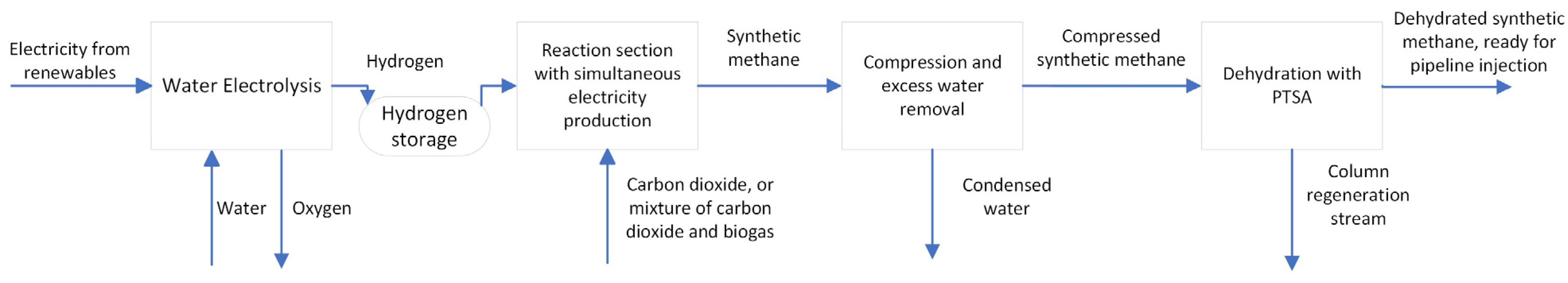
The process scheme for the P2M process is illustrated roughly in Figure 1. The final process scheme was generated in Aspen Plus, with the help of the process schemes from Tripodi et al. [15], Whalen [22] and Müller et al. [23].
First, hydrogen is produced via water electrolysis, using electricity from renewable sources. Hydrogen is then stored temporarily. The produced hydrogen and CO2 are consumed in the methanation part of the process, to produce synthetic methane, which can then be compressed, dehydrated via PTSA and injected into the pipeline. The reaction section, compression and a simple model of the PTSA were simulated in Aspen Plus. More rigorous simulation of PTSA was carried out in Aspen Adsorption. Only a simple calculation of the water and electricity requirement was carried out for electrolysis. The amount of produced oxygen was also determined.
The process scheme used for the simulation in Aspen Plus is shown in Figure 2. These are the methanation part, shown by purple process streams; the thermal fluid (TF) cycle, shown by red process streams; and the steam cycle, shown by blue process streams.
2.3.1. Electrolysis
In electrolysis, water is split by the reaction shown in Equation (6), forming oxygen (O2) and hydrogen. Electrolysis would not run in a steady state and at the same time as the methanation process. The operation of electrolysis is economically reasonable only in times of low electricity prices on the market. For the chemical process, it is desirable to ensure a constant supply of hydrogen. For this reason, the operation of the electrolysis plant must be flexible. In order to decouple the two stages of the P2M process, intermediate storage of the hydrogen can be a viable solution [24]. At low prices, the maximum hydrogen production rate of electrolysis must, therefore, be higher than the consumption rate of hydrogen in the methanation section. Thus, methanation can operate, even at times that are not optimal for hydrogen production. For the process in this study, we have assumed three times the hydrogen production capacity of the electrolysis plant, considering possible losses of the stored hydrogen. According to Genovese et al. [25], up to 1% of the hydrogen mass per day can be lost. If we consider that the hydrogen could be stored for 3 days, the electrolysis at 100% operating capacity, including the assumed losses, would have to produce 1553.34 kg/h of hydrogen.
The required capacity of the electrolysis plant was calculated using the known hydrogen flow rate. It was considered that there are three types of electrolysers that are currently established on the market. These are alkaline (AEC), proton exchange membranes (PEMs) and solid oxide electrolysers (SOECs). Each of these types have different efficiencies [24], which also affects the required electrical power rating of the electrolysis plant if the same hydrogen production capacity is to be guaranteed.
The capacities required for the different types of electrolysers are given in Table 3. The efficiencies are taken from the Sunfire and Nel catalogues. Sunfire produces AEC and SOEC and Nel produces AEC and PEM electrolysers [26,27]. The required water flow and oxygen flow that would be produced at full operation capacity was calculated using Equation (6) and the required hydrogen flow rate. The calculated produced O2 flow was 12,303.84 kg/h, while the production required 13,857.20 kg/h H2O.
2.3.2. Methanation
The methanation section is dedicated to CO2 methanation. It was assumed that the H2 and CO2 were already under pressure before they entered the process. In the case of simultaneous methanation, we assumed that the biogas must be compressed to operating pressure. That was done with a two-stage compressor, MC-1, with intermediate cooling to 30 °C.
The reactants first pass through the heat exchanger HE-1, where they are preheated to 290 °C by the product stream RP-1. Then, they enter the reactor R-1, where the Sabatier reaction takes place. The products are first cooled as they flow through the HE-1. Further cooling in the heat exchanger HE-2 provides heat for water preheating in a modified Rankine cycle (RC). Lastly, cooling to 30 °C is carried out with cooling water at 20 °C. This condenses the water in the gas flow. The separation of the two phases is carried out in process unit F-1. The vapour phase is preheated to 290 °C in the exchanger HE-4, along with the products of the second stage. The vapour phase then enters reactor R-2.
Due to the heat emitted to preheat the process stream S-6, the RP-2 stream is partially cooled. Additional cooling to 30 °C is carried out in HE-5 with cooling water. The condensed water is removed in the separator F-2. The vapour phase is compressed to 51.1 bar with a two-stage compressor, MC-2, with intermediate cooling to 30 °C. The synthetic methane that leaves the compressor is cooled to 25 °C in HE-6. Before the stream enters PTSA, the condensed water is removed in F-3. The stream phase is then dehydrated via PTSA, which is explained in Section 2.3.3.
The TF flows into the reactor R-2 at 285 °C and is heated to 349 °C while it flows through the reactor R-1. Such temperatures ensure that the conversion of CO2 in both reactors is near equilibrium, which is specific for the operating temperature and pressure. The received reaction heat is released through a series of heat exchangers, MPW-H, MPS-G and SHMPS-G, which are designed to generate medium-pressure steam. In both reactors, the TF stream flows concurrently with the reaction mixture.
In the software, the isentropic efficiency of the two two-stage compressors was set to 85.6% and the mechanical efficiency was set to 99.6%, in accordance with Pan et al. [28]. For the heat exchangers HE-1, HE-2 and HE-4, model HeatX was used, while HE-3, HE-5 and HE-6 were modelled with a heater model. In the heater model, built-in cooling water was selected as the cooling utility. Aspen Plus uses water inlet and outlet temperatures of 20 and 25 °C, respectively. Intermediate cooling in the compressors uses the same cooling utility. F-1, F-2 and F-3 are adiabatic gas–liquid phase separators, which have been modelled with the Flash2 model available in Aspen Plus.
The reactors are multi-tube, plug flow reactors modelled with RPlug. The first reactor contains 40 kg of catalyst, while the second reactor contains 150 kg. The reactor has 253 tubes, 3 m in length and 50 mm in diameter. The heat transfer coefficient between the TF and reactants was estimated to be 850 W/(m2K) using Aspen Plus.
The heuristics were used to estimate the pressure drops in the process units. For gases in the heat exchangers, we assumed a drop of 0.20 bar, for the condensing or vaporising process streams, we used a value of 0.10 bar and for the water process streams in the modified RC, we used a value of 0.35 bar. We assumed a drop of 0.15 bar for the interstage compression and a drop of 0.2 bar in the reactors. Accordingly, the process operated at an inlet pressure of 6.3 bar. Through the methanation section, the pressure drops to 5 bar (stream S-11). The first reactor thus operates between 6.1 and 5.9 bar, while the second reactor operates between 5.5 and 5.3 bar. The pressure drops have been neglected for the TF streams.
A simple stream splitter model was used for the PTSA unit in Aspen Plus. The results of a dynamic simulation of the PTSA unit, simulated in Aspen Adsorption, were used for the split fractions of the components.
2.3.3. Modified Rankine Cycle
For the simultaneous generation of electricity, a modified RC was included in the scheme. The cycle was adopted from Garuge [29]. In the cycle, a series of heat exchangers, MPW-H, MPS-G and SHMPS-G, generate medium pressure steam at 14.2 bar and 345 °C. Superheated steam enters the turbine T-LP1, through which the pressure drops to 1.5 bar. The steam flows out of the turbine near saturation, after which it is superheated to 337 °C and fed into turbine T-LP2. In this turbine, the pressure drops from 1.3 bar to 0.0352 bar. The saturated steam is condensed at vacuum pressure, the water is pressurised by pump RC-P, preheated to 130 °C by heat exchanger HE-2 and recycled back into the RC.
The pump and turbines, like the compressors, have an isentropic efficiency of 85.6% and a mechanical efficiency of 99.6%. The heat exchanger CT is modelled with a simple heater model. The condensation is carried out with cooling water. For the other heat exchangers in the RC, the HeatX model was chosen.
The pressure drops were determined by heuristics, as described in Section 2.3.1. The pump raises the water pressure to 15.20 bar, which drops to 14.2 bar by the time it enters the first turbine. The RC used is shown in Figure 3 with a temperature–entropy (T-s) diagram.
2.3.4. Synthetic Methane Dehydration
The dehydration of the product stream PROD-2 was performed via dynamic simulation of the PTSA in Aspen Adsorption. To perform the simulations, we adopted isothermal data on the adsorption of CH4, CO2 and H2O on silica gel from Grande et al. [30]. A Langmuir–Freundlich model, with temperature dependence of the affinity kept constant, was fitted to the data by minimising the residual sum of squares (RSS). The calculation of the RSS is shown in Equation (7) [31], and the isotherm model in Equation (8) [27]. The model was fitted to the data, using the Excel solver and the global minimisation macro GlobalMinimize, developed by Schild [32].
where yi is the adopted experimental value and f(xi) is the model predicted value [31]. qe, k is the amount of component k adsorbed in equilibrium. Parameters qm, k; b∞,k; nk and Qads, k present the saturation capacity, affinity constant at infinite temperature, empiric heterogeneity parameter and heat of adsorption for species k [33].
The obtained Langmuir–Freundlich parameters are shown in Table 4, while the predicted isotherms on the experimental data are shown in Figure 4.
With the obtained isothermal parameters, the calculation of the Langmuir–Freundlich model parameters (IP), suitable for the Aspen Adsorption, was carried out as shown in Table 5. The obtained parameters are shown in the units suited for the software [34]. The calculated parameters of the pure components were used in the program, while the Langmuir–Freundlich model was chosen to describe the equilibrium. This model predicts the behaviour of the multi-component system from the pure component isotherms [34].
The program also required data on the adsorbent and mass transfer. The provided data are shown in Table 6. We also included a rigorous heat transfer in PTSA, and therefore, the data used for heat transfer are also shown.
For adsorption, we did not consider the adsorption of H2 and CO, which is why we set the values for kLDF to 0. This way, they are considered in molar flows for simulation, but they are not adsorbed, since the literature did not provide its adsorption isotherms. Even if both pass through the column, their molar fraction in the final dehydrated synthetic methane is still within the relevant standards.
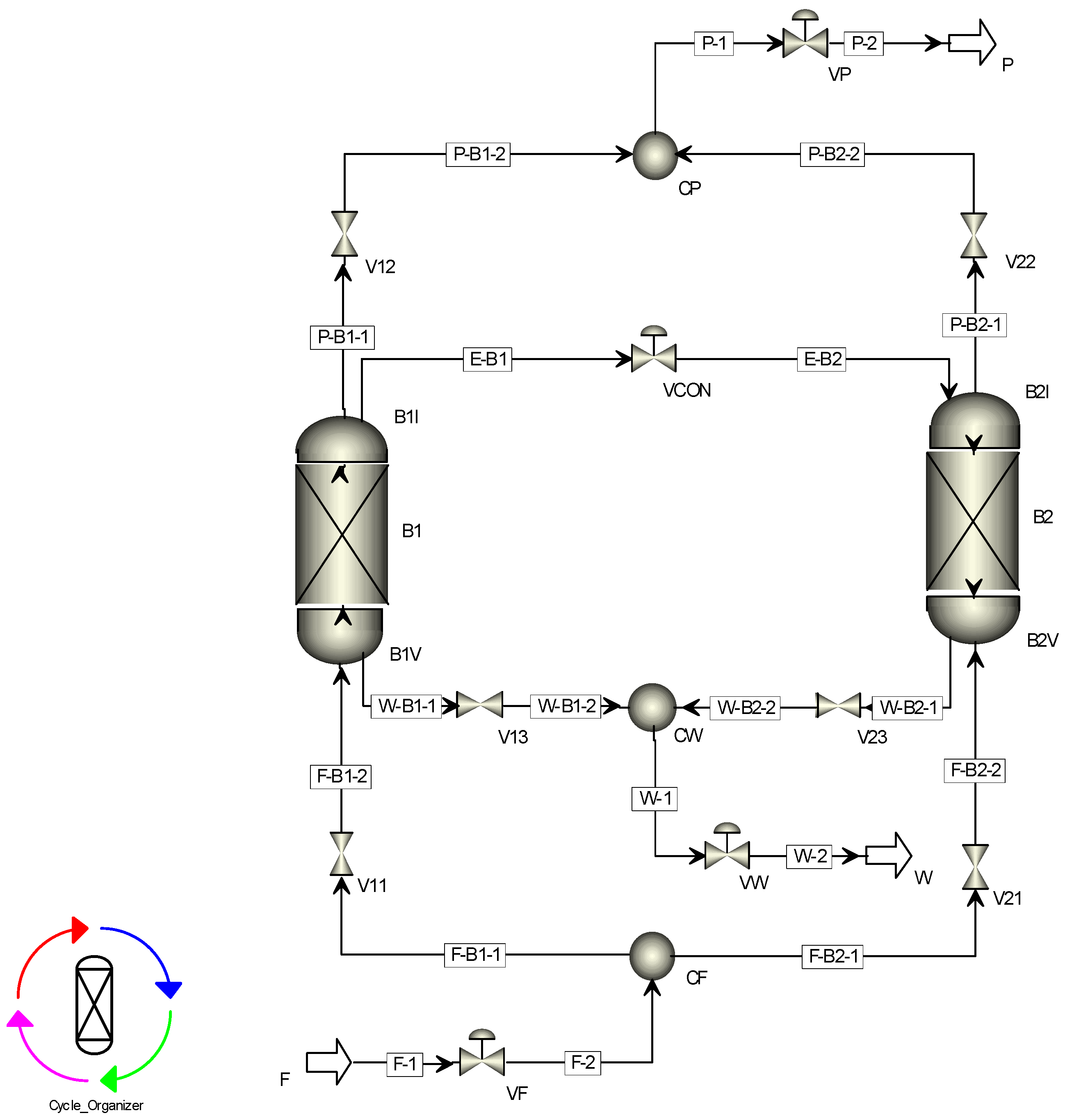
Using the data given in Table 5 and Table 6, a 6-step PTSA dehydration of synthetic methane was simulated with adsorption process shown in Figure 5 and the process scheme shown in Figure 6. During regeneration, the regenerating column was heated with a water flow rate of 2 kg/s at a temperature of 100 °C.
In a 6-step pressure swing adsorption (PSA) cycle, two columns operate in parallel. The principle of operation is illustrated in Figure 5. In step i, the adsorption takes place in column B1, while column B2 is regenerated with a fraction of the product, which passes through the column. When column B1 is saturated, the feed is stopped until the pressure between the two columns is equalised (step ii). In step iii, column B1 is de-pressurised, while column B2 is re-pressurised with the feed. Steps iv, v and vi proceed in the same way, but with the reversed role of the adsorption columns [35]. Steps ii and v are designed to save energy, as part of the pressure change is provided automatically when the flow between the columns is established. In steps iii and vi, required work for the compression to raise the pressure in the column is therefore reduced [43]. The 6-step PTSA cycle used in this study operates in the same way. The only difference is that additional heating was used in regeneration steps.
2.4. Analytical Methods
2.4.1. CO2 Conversion and CO Selectivity
The CO2 conversion () was calculated from the flow rates of CO2 () at the inlet and outlet of the reactor, or the whole process scheme, using Equation (9). The flow rate of CO () in the outlet of the reactor, or the whole scheme, was used to determine the selectivity of CO (SCO), using Equation (10) [18].
It is worth pointing out that when we talk about the conversion or selectivity of the overall process, these are calculated in relation to the total CO2 input and the total CO2 or CO flow rate in the PROD-2 stream. That way, the losses in stream W are not subtracted.
2.4.2. Losses of Methane in PTSA
The methane losses () in a dynamic dehydration simulation were determined with Equation (11). The net moles of methane, lost in stream W during the elapsed operating time (), and the total amount of methane that entered with stream F () were determined first in the calculation. The total amounts of both streams were calculated with the adapted middle Riemann sum, shown in Equation (12) [44]. The dynamic data of the total flow rates of process streams i, at times j (), and the corresponding mole fractions of methane () were obtained from the Aspen Adsorption. The data were recorded with a time interval of 400 s, and the total elapsed time (tp) corresponded to 10 cycles of operation.
2.4.3. Steady-State Operation of PTSA
In order to use the results of the dynamic operation in Aspen Plus, we first determined the time variation of the average composition () and the process flow rate, i (), at time tp, using Equations (14) and (16). Here, tp represents the elapsed time of operation of the PTSA, from time 0 to the selected time p, where the maximum time is the time at which the 10th cycle of operation is completed. represents the total amount of stream i entered, or exited, from the PTSA in a selected time frame (from time 0 to tp). Similarly, represents the total moles of component k [44]. and were determined by Equations (13) and (15).
After sufficient time has passed, the average compositions and flow rates, determined with Equations (14) and (16), converge to relatively constant values. With these, we can define a steady-state operation. The obtained values were obtained by averaging the and from day 40 onwards. From the steady-state compositions () and flow rates (), the split fraction of each component k () was determined using Equation (17) [44]. This is the fraction of component k that passes from the stream, PROD-2, to the final, dehydrated stream of synthetic methane, SYNCH4. The split fractions were used in Aspen Plus to model the PTSA unit.
Equations (13) to (16) can also be used to determine the average temperature of the product and waste streams. In this case, is replaced by , which represents the integral of the temperatures from time 0 to time tp. and are replaced by and to represent the temperatures at time j and j-1, respectively. The average temperature of stream i at time tp is obtained by replacing with in Equation (14). The steady-state temperature of the stream i is then determined by averaging from day 40 onwards.
2.5. Simulation Procedure
The process was simulated in Aspen Plus. First, the simulation without PTSA was run to obtain the flow rate and composition of the product stream, PROD-2. With known composition and flow rates, a dynamic dehydration simulation was run in Aspen Adsorption to obtain the steady-state compositions, flow rates and temperatures of the process streams P and W in the scheme of Figure 6. The split fractions of the individual components that pass from the input mixture F to the product stream P were calculated. These were used in the Aspen Plus, in the PTSA unit, which was modelled as a simple flow splitter. The process in Aspen Plus was then run again.
In both Aspen Plus and Aspen Adsorption, the Peng–Robinson equation of state was used to describe the physical properties of the mixtures.
The dynamic dehydration simulation was performed only for the product stream of the first case. Ten cycles of PTSA operation were performed. For the second case, the same split fractions were used in the PTSA in Aspen Plus.
Certain constraints and assumptions were used in the simulations:
- Only three components were considered for biogas, namely, CO2, CH4 and H2O.
- All simulations were limited to data obtained from the literature.
- The P2M process operated continuously in a steady state.
- The P2M process was not optimised.
- No heat was lost in the methanation section of the P2M process.
- The mechanism of the Sabatier reaction assumed that CO2 first reduces to CO.
- The possible conversion of CO to C was neglected.
- Other possible side reactions were also neglected.
- No condensation of steam occurred in the turbines.
- All gas–liquid separators operated adiabatically with no pressure drop.
- The adsorption of H2 and CO was not considered in dehydration.
- No reaction between the gas phase and adsorbent took place in PTSA.
3. Results and Discussion
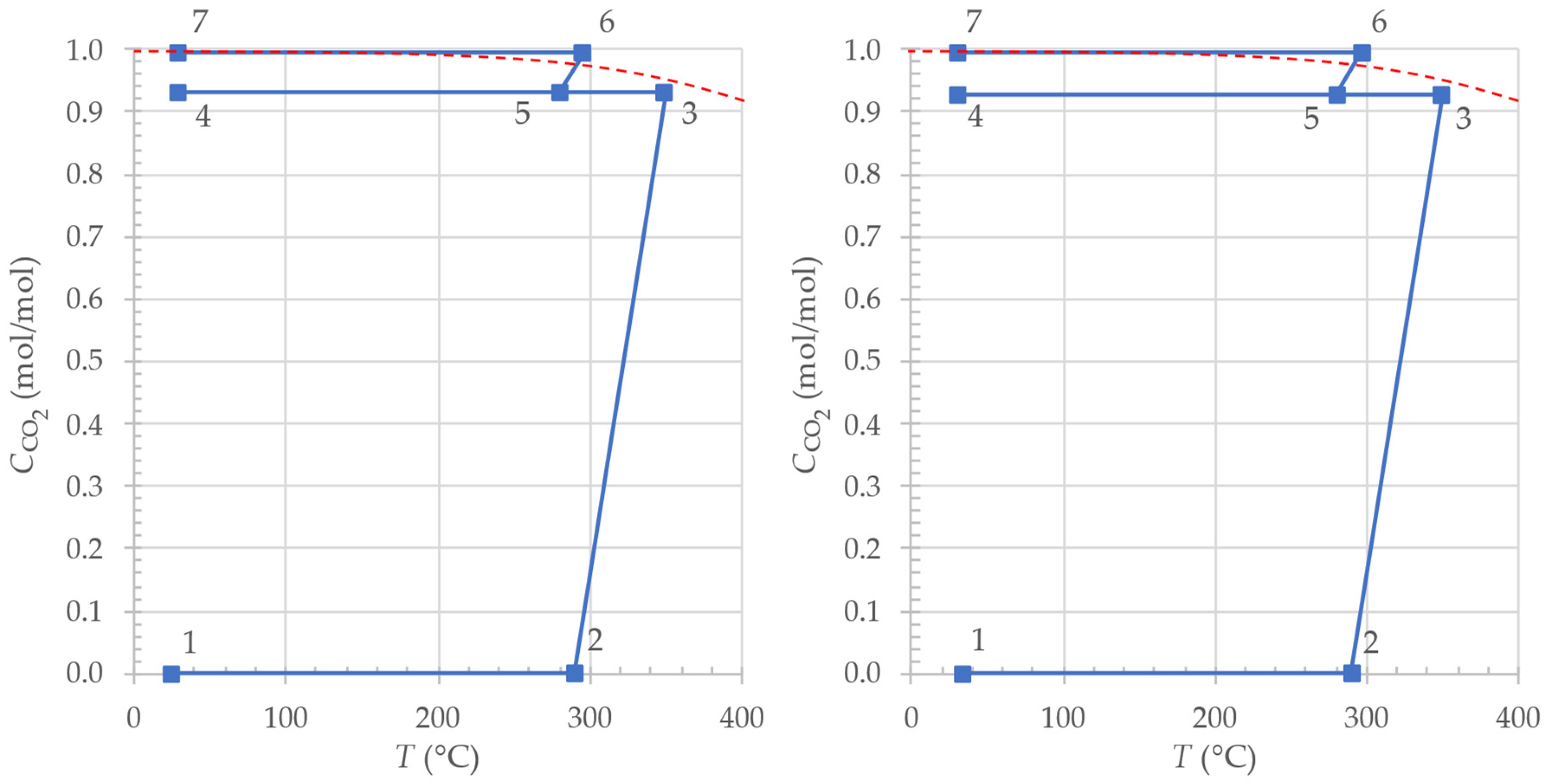
In the first case, the total CO2 conversion was 99.43%, while in the second case, it was 99.33%. In the methanation of the first case, higher conversions are achieved due to the Le Chatelier principle, which states that the system responds to the addition of reactants by lowering the concentration of the reactants in equilibrium [45]. Since CH4 is a product of the methanation reaction and is already present in the reactant stream at the beginning, the equilibrium effects lead to the formation of a smaller amount of products. In a similar way, the removal of products shifts the equilibrium of the reaction in the direction of the products [45]. Cooling of the product stream between the reactor stages was implemented for this reason. If one looks at the Sabatier reaction shown in Equation (1), it can be seen that for 1 mol of CH4 produced, 2 mol of H2O is produced. The maximum CO2 conversion is limited by the equilibrium. However, because a lot of water is produced, its condensation from the product stream allows higher CO2 conversions in the second reaction stage. With a sufficiently large number of reaction steps with intermediate cooling, CO2 conversions up to even 100% are possible [15].
Figure 7 shows the conversion–temperature path of the process. It is important to note that lines 2–3 and 5–6, representing reactors R-1 and R-2, respectively, do not show the actual profile of conversion in the reactor, but only the conversion of CO2 at the inlet and outlet of the reactors. Point 1 represents the temperature of the S-2 stream, the point 4 represents S-6 stream and the point 7 represents S-9 stream. The temperature is higher in case 2, due to the compression of the biogas, which heats the biogas stream in the second compression stage.
3.1. Temperature and Concentration Profiles
The issue of the formation of a hot spot in the first reactor arises. When the simulation was carried out with a 120 kg catalyst, the peak temperatures reached as high as 600 °C. By lowering the mass to 40 kg, the temperature was reduced successfully, but Figure 8 shows that the hot spot was still present. Lowering the catalyst mass further led to simulation errors.
The formation of the hot spot was caused by a rapid consumption of reactants in the initial lengths of the reactor, as shown in Figure 9. The hot spot was therefore formed at 1.8 m. At the same location, we observed higher CO fractions. In the adopted model, it is assumed that CO2 methanation takes place via an intermediate reduction to CO, via the RWGS reaction. This reaction is endothermic, with a standard reaction enthalpy (ΔrH°) of 41 kJ/mol, while CO methanation is exothermic, with ΔrH° = −206 kJ/mol [15]. We concluded that the large amount of heat released during the methanation of CO accelerates the RWGS reaction greatly, while the high temperature makes it more difficult to convert the formed CO further. Because of that, it accumulates in the vicinity of the hot spot. This accumulation can lead to a further reduction of CO to carbon [20]. This causes a build-up of the active surface of the catalyst, and, with time, leads to a loss of catalytic activity [46]. In the simulations, we have neglected this, which is why the CO was still converted to CH4. It would make sense, however, to remove the hot spot and consider possible coke formation in further simulations. To eliminate hot spots, inert material is mixed with the catalyst. Moreover, less catalyst is applied in the initial parts of the reactor [47]. Aspen Plus, however, does not have a built-in function to add inert material, or to determine a custom distribution of the catalyst mass along the reactor.
In the second reactor, the reactions are also fast, but no hot spot was observed, because much smaller amounts of CO2 and H2 were reacting. Figure 8 also shows the temperature profile of the TF in the reactors.
3.2. Synthetic Methane Dehydration
A six-step cycle was used to simulate 10 dehydration cycles of operation. For each step in the PTSA cycle, the specifications for all valves are presented in Table 7. In addition, it is shown in which steps of the cycle the column heating was switched on. Table 8 shows the-time driven PTSA operation. It also shows the operating pressures and the temperature at which regeneration occurred. Final results are shown in Table 9.
After carrying out the simulation of the first case in Aspen Plus, we obtained the composition of the PROD-2 stream, which is presented next to the other process streams in Table 10. A dynamic adsorption simulation was performed with the results. Unless otherwise noted, all results in this section refer to the dehydration of the PROD-2 stream, produced with the methanation of pure CO2. The justification for using the same split fractions for the dehydration of both cases is discussed at the end of this chapter.
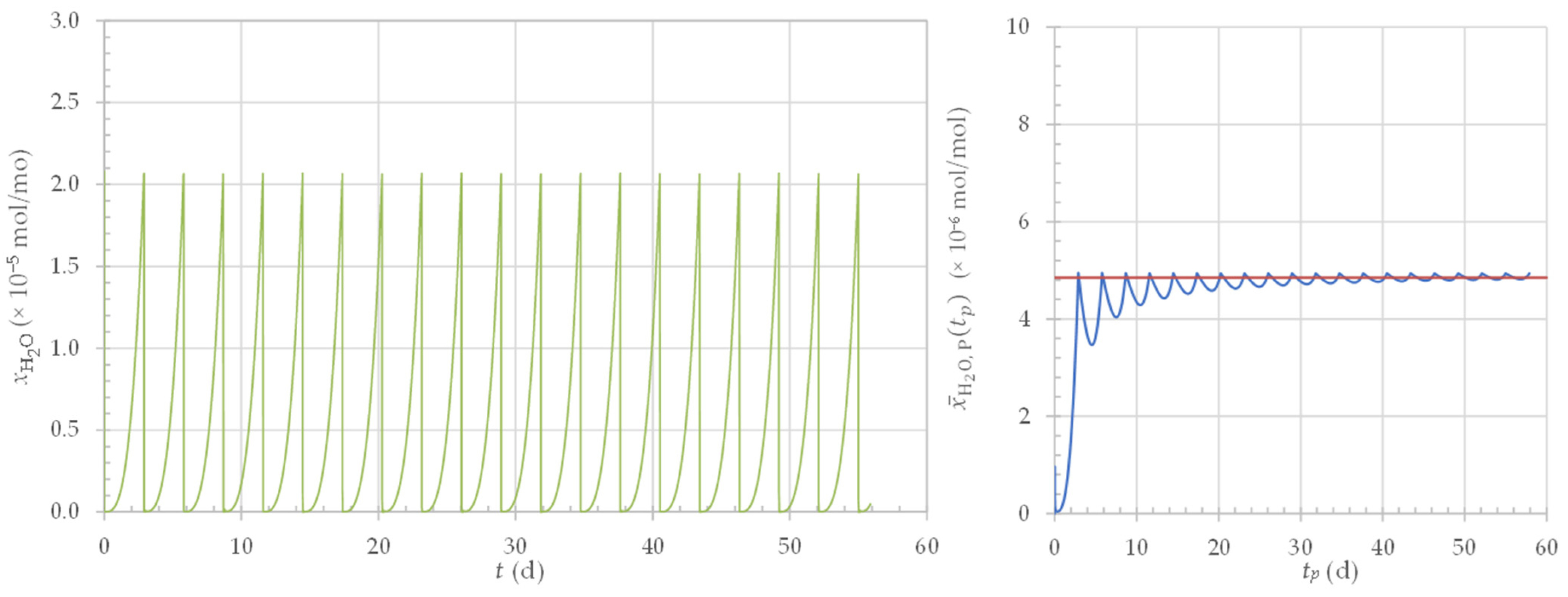
The simulated dehydration PTSA ensures a sufficiently low water content in the dehydrated synthetic methane to meet many pipeline standards of different European countries, as given by Awe et al. [11]. Figure 10 shows how the water fraction and average water fraction in the product stream varies with time. The maximum water fraction in the product stream was 0.00208 mol.%. The determined steady-state value of the average water fraction in the product stream is represented by the horizontal red line. The other steady-state compositions are shown in Table 9, together with the calculated split fractions.
The steady-state temperatures of the product and waste streams have also been transferred to Aspen Plus. The product stream has warmed up slightly due to the adsorption process in the column. The determined steady-state flows and temperatures were:
- = 1.7680 × 10⁻² kmol/s;
- = 1.7562 × 10⁻² kmol/s;
- = 1.1848 × 10⁻⁴ kmol/s;
- = 298.15 K = 25.00 °C;
- = 298.97 K = 25.82 °C;
- = 371.32 K = 98.17 °C.
According to the split fractions, the methane losses in the PTSA are very low, since 99.42% of all methane from the PROD-2 stream passes into the SYNCH4 stream. According to the second equation, we determined the losses to be 0.57 mol.%. Consequently, the effluent flow rate W was also very low, as can be seen in Table 10. Such low losses are achieved because only a small fraction of the product stream is passed through the regenerating column. Although this results in long column regeneration times, the chosen column dimensions enable long operating cycles. The column regeneration time for the first cycle is shown by the blue dotted line in Figure 11.
Via dynamic simulation, we determined that the PTSA dehydration system requires a heat flow of 3.99 kW. The value was obtained by summing the amount of heat exchanged with the heating water for both columns, and then dividing the value by the operating time of the whole system.
For the PROD-2 stream from case 2, cyclic operation was not repeated. Instead, we simulated only the breakthrough curve for the composition and flow of the second case and saw that the use of the dehydration results of the first case was justified.
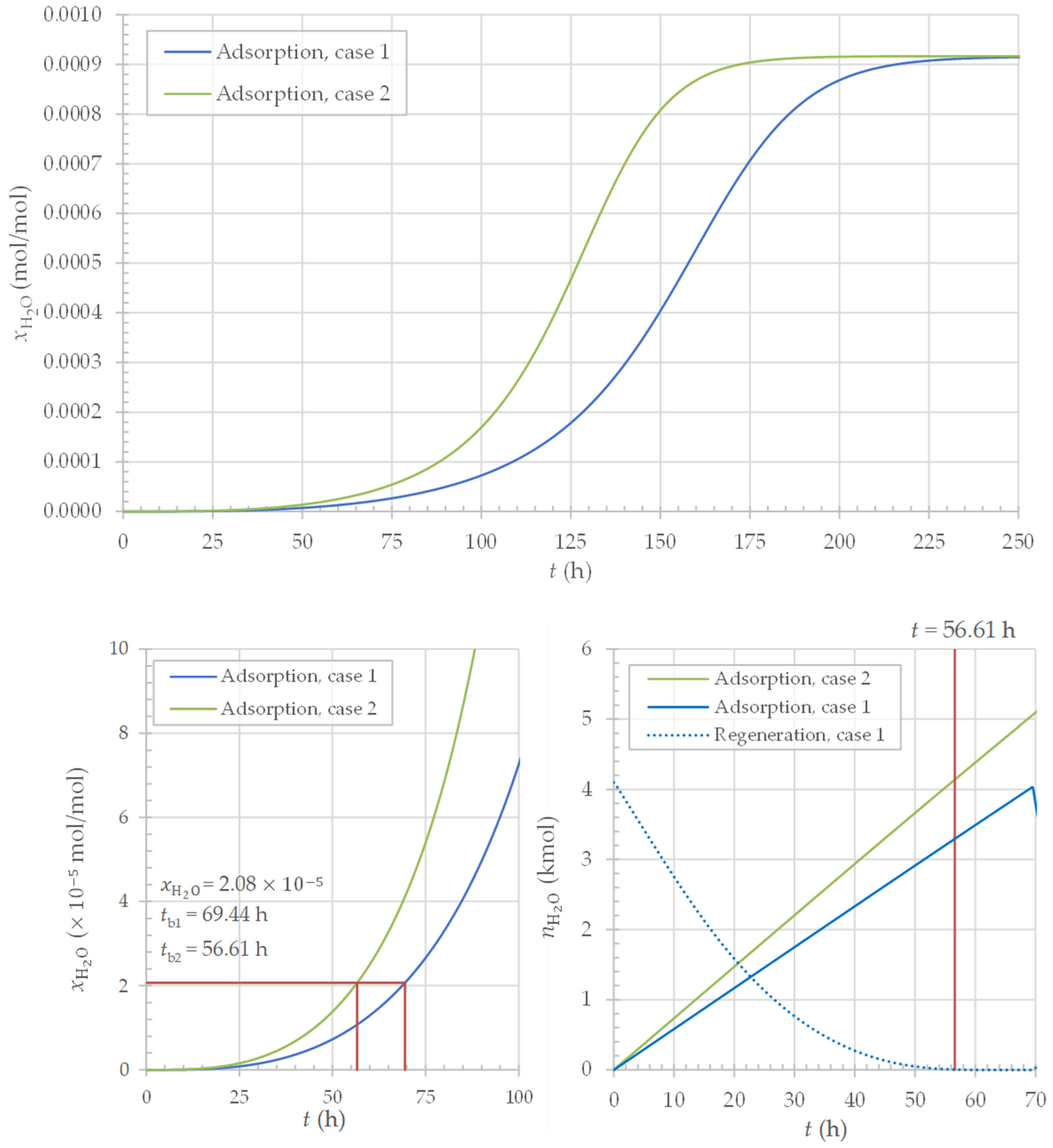
The solid blue line in the upper diagram in Figure 11 shows the breakthrough curve for the dehydration in the first case. The flow rate of the PROD-2 stream was higher when dealing with the dehydration of synthetic methane produced by simultaneous methanation. Since the column dimensions were the same in both cases, the breakthrough was therefore achieved more quickly.
To ensure the same maximum water fraction in the product in the dehydration of case 2, the adsorption and desorption times of the columns must be reduced to 56.61 h due to the higher flow rates. From the diagram on the right, approximately the same amount of water would be adsorbed in the column at this time. Since the amount adsorbed is very similar, we assume that this amount would also be desorbed in a very similar time. The time for desorption of such an amount of water can be estimated to 54 h from the blue dotted line on the bottom right diagram. This is sufficiently fast, as the desorption time does not exceed the adsorption time. Therefore, we concluded that the same split fractions can be used for the dehydration of both cases. The expected flow rate and composition of the SYNCH4 stream from case 2 are given in Table 11.
3.3. Process Stream Results
Table 10 and Table 11 show the final temperatures, pressures, flows and compositions of all process streams for the simulated synthetic methane production. Table 10 shows the results of the first case and Table 11 the results of the second case.
We have simulated the production of synthetic methane successfully. The flow rate of the PROD-2 stream from case 1 was 1013.49 kg/h and corresponds to a calculated pure methane flow rate of 1 t/h. There were minor losses in the PTSA unit, resulting in a final product flow of the SYNCH4 stream of 1006.55 kg/h. In the waste stream of the PTSA unit, 5.75 kg/h of CH4 was lost. Given that the methane flow rate in the PROD-2 stream was 993.85 kg/h, only 0.58% of methane was lost. The value corresponds to the losses predicted by the dynamic PTSA simulation.
The case 1 composition of the SYNCH4 stream corresponds to the literature standards for natural gas pipelines provided by Awe et al. [11]. The exception is Sweden, because the hydrogen fraction in the final stream is too high. From Aspen Plus, we have also obtained the Wobbe Index on a volume basis at a reference temperature of 0 °C. The Wobbe Index of the SYNCH4 stream is 52.75 MJ/m3. In some cases, this is too high. For example, the Netherlands requires upper index values between 43.46 and 44.41 MJ/Nm3. Accordingly, the minimum required CH4 fraction is also lower, at 85 mol.% [11]. To lower the Wobbe Index, the synthetic methane product stream could, in such cases, be blended with nitrogen.
Although the CO2 conversions are lower in case 2, the methane fraction of the product is higher. We conclude that this is due to the initial methane content, which raises the methane content of the product. The case 2 compositions of the final stream are within the relevant standards, and the Wobbe index is 52.82 MJ/m3. Due to the initial methane content, the final synthetic methane flow rate is slightly higher, at 1274.53 kg/h. The methane losses in the PTSA are, therefore, also higher (7.30 kg/h), but amount to the same percentage of lost methane (0.58%). It makes sense that the losses are the same, as we have assumed that the split fractions of the PTSA unit in Aspen Plus are the same for both cases.
Methane losses also occur during condensation. Due to dissolution in water, methane is also removed from the process with streams WW-1, WW-2, WW-3, WW-4 and WW-5. It can be seen from Table 10 and Table 11 that these losses are very small. Primarily, the streams are composed of water, the fraction of which ranges from 99.996 mol.% to 99.999 mol.%.
During simulations, it was found that the process is flexible in operation. In cases when surplus power is not available, the process can operate in a hot standby, where small amounts of reactants are consumed. The production of synthetic methane adapts to the hydrogen production. In this case, the process can operate at a lower pressure. When surplus electricity becomes available again, it is used to produce the hydrogen via water electrolysis. The pressure can be increased simultaneously, which expands the capacity of the process. Higher pressure also increases the maximum achievable CO2 conversions, since they are limited by the reaction equilibrium. In cases, where the CO2 content in the final product is too high, its removal would be necessary. The use of higher pressures in our study ensures a sufficiently high methane content. The process, therefore, does not require the upgrading of technologies for CO2 removal, such as water scrubbing, which consumes large quantities of water.
3.4. Energy Streams in the Process Units
Table 12 shows the work and heat flows of the process units for both cases. In the table, we first show the amount of electricity consumed at 100% operating capacity of the three types of electrolysers. The AEC has the highest consumption and the SOEC the lowest, as the latter has the highest efficiency of the three.
With multi-stage compression in the MC-1 and MC-2 units, there is an intermediate cooler between the stages. Its heat flow is expressed as a negative value, because the heat is released to the cooling water. For this reason, in process units where cooling water is present, its consumption is given as a mass flow rate (). As the heat exchangers HE-3, HE-5, HE-6 and CT are also cooled with water, the table shows the negative value of the heat flows and the water consumption for cooling.
For the reactors R-1 and R-2, the negative value represents the heat released in the reaction. The heat is removed from the reactor by the TF flow. In other heat exchangers, the positive values are given for the heat flows. This indicates the heat exchanged between the process streams.
The PTSA is a heat sink. During regeneration, the columns are heated at a water flow rate of 2 kg/s at 100 °C. This flow could be provided with the heat exchanger HE-3, where the water would be heated from 20 °C to 100 °C. With the equation , we can calculate that, in case 1, when less heat is released at the heat exchanger, a water flow of 2.83 kg/s could be guaranteed. In this calculation, we used a temperature change of ΔT = 80 K and a specific heat capacity for water of cp = 4 182 J/(g⋅K). The result of the dynamic simulation of the PTSA unit showed that only 3.99 kW of heat is exchanged during regeneration. The low heat consumption means that the outlet temperature of the heating water is only slightly lower than the inlet temperature. This was confirmed by the average temperature of the heating water at the outlet of the column. On average, the water that passed through the columns was cooled by only 0.49 °C.
There is not much additional potential for heat integration in the process scheme, as the only heat sink in a steady-state operation is the preheating of the reactant. This integration is already ensured with exchangers HE-1 and HE-4. Although PTSA requires heat, the required heat flow is practically negligible compared with the other heat flows in the P2M process.
Instead of heat integration, it is possible to implement cogeneration or simultaneous electricity production. A large part of the heat released in the methanation process is already used to produce superheated medium-pressure steam, which is used to generate electricity in the turbines. In the RC, the CO2 methanation produces 946.67 kW, but when biogas is mixed at the inlet, the work produced is lower, at 938.87 kW. The lower value is to be expected, as the overall CO2 conversion is lower in the case of simultaneous methanation. As a result, overall, less heat is released in the reaction, and the amount of steam produced is therefore lower, but the change does not have a significant impact on the required pump work, which, in both cases, amounts to 1.69 kW.
According to the results in Table 12, the methanation stage is still a large consumer of cold utilities. Large quantities of cooling water are required for the intermediate cooling in two-stage compressors and in the heat exchangers HE-3, HE-5 and HE-6. To reduce, or even eliminate, the consumption of cold utilities in the methanation section further, this heat could be used to produce hot sanitary water.
There is also the possibility of introducing another level of low-pressure steam in the steam cycle. This would increase the amount of produced electricity. The introduction of an additional level would make use of the heat and shift the cooling water consumption from the methanation section to the steam cycle, where it would be used to condense the saturated steam. It can be seen from the table that the condenser CT, which is used to condense vacuum steam, consumes large amounts of cooling water. The introduction of a new cycle would increase the water consumption further. The released heat cannot be used directly in any other way, as it is low-temperature heat at 31 °C.
Due to the high consumption, the operating costs of the electrolyser can also be very high. To cover even a small amount of the needed electricity, it would be reasonable to improve the co-generation of electricity in further simulations.
As the simultaneous generation of electricity results in an additional investment due to the required process units, it would also be reasonable to carry out an economic analysis of the different process configurations.
It is important to highlight the special case of using SOEC for hydrogen production. The SOEC must be operated at sufficiently high temperatures to ensure a proper electrolysis operation. Heat can be supplied by using the released reaction heat to produce water vapour. The vapour is then used in the electrolysis to produce hydrogen [8]. The electricity consumption is reduced, because a part of the energy needed for the electrolysis is provided by heat [19]. For this reason, it would also be worthwhile to investigate the possibility of integrating SOEC and the methanation section of the P2M process further.
4. Conclusions
A partially integrated process for the production of synthetic methane through CO2 methanation was simulated in the study. The process’s potential lies in seasonal energy storage, where large amounts of surplus renewable energy can be stored with low losses for long periods of time.
We have shown that the process is capable of both pure CO2 methanation and methanation of a mixture of biogas and CO2. High CO2 conversions were achieved, averaging 99.38%. With a high methane content of 97.33 mol.%, the product is suitable for injection into natural gas pipelines. The process has not been optimised, and additional heat recovery and water integration is still needed.
The results are promising, but the process itself has some challenges to overcome. It is limited by CO2 transportation to the site and electricity prices on wholesale markets. Current limitations are the high investment costs of electrolysers, its efficiencies, and operational costs due to its high electricity consumption. Nevertheless, it is expected that those limitations would, to some point, be resolved as the technology matures.
Author Contributions
Conceptualisation, methodology, software, validation, investigation, formal analysis and writing—original draft: K.R.; investigation, formal analysis and writing—original draft: S.G.; formal analysis, writing—review and editing and supervision: D.U.; supervision: D.G. All authors have read and agreed to the published version of the manuscript.
Funding
This research received no external funding.
Data Availability Statement
Not applicable.
Conflicts of Interest
The authors declare no conflict of interest.
Abbreviations
| AEC | Alkaline electrolytic cell |
| LDF | Linear driving force |
| LHHW | Langmuir–Hinshelwood–Hougen–Watson |
| PEM | Proton exchange membrane |
| PSA | Pressure swing adsorption |
| PSRK | Predictive Soave–Redlich–Kwong |
| PTSA | Pressure–temperature swing adsorption |
| P2G | Power-to-gas |
| P2M | Power-to-methane |
| RC | Rankine cycle |
| RWGS | Reverse water gas shift |
| SOEC | Solid oxide electrolyser cell |
| TF | Thermal fluid |
References
- Power-to-Methane: Current Scenario in EU. Available online: https://www.futurebridge.com/industry/perspectives-energy/power-to-methane-current-scenario-in-eu/ (accessed on 21 August 2023).
- Record Growth in Renewables Achieved Despite Energy Crisis. Available online: https://www.irena.org/News/pressreleases/2023/Mar/Record-9-point-6-Percentage-Growth-in-Renewables-Achieved-Despite-Energy-Crisis (accessed on 23 July 2023).
- Power-to-Gas. Available online: https://nelhydrogen.com/market/power-to-gas/ (accessed on 16 July 2023).
- Amelang, S.; Appunn, K. The Causes and Effects of Negative Power Prices. Available online: https://www.cleanenergywire.org/factsheets/why-power-prices-turn-negative (accessed on 23 July 2023).
- Andersson, J.; Grönkvist, S. Large-Scale Storage of Hydrogen. Int. J. Hydrogen Energy 2019, 44, 11901–11919. [Google Scholar] [CrossRef]
- What Is Hydrogen Storage and How Does It Work? Available online: https://www.twi-global.com/technical-knowledge/faqs/what-is-hydrogen-storage.aspx (accessed on 16 July 2023).
- Hydrogen or Methane? Available online: https://edenergy.be/hydrogen-or-methane/?lang=en (accessed on 14 September 2023).
- Van Leeuwen, C.; Zauner, A. Innovative Large-Scale Energy Storage Technologies and Power-to-Gas Concepts after Optimisation; University of Groningen: Groningen, The Netherlands, 2018; p. 51. [Google Scholar]
- Biogenic CO2 Is on of Our Green Solutions. Available online: https://www.green-create.com/green-solutions/biogenic-co2/ (accessed on 23 July 2023).
- Calbry-Muzyka, A.S.; Schildhauer, T.J. Direct Methanation of Biogas—Technical Challenges and Recent Progress. Front. Energy Res. 2020, 8, 570887. [Google Scholar] [CrossRef]
- Awe, O.W.; Zhao, Y.; Nzihou, A.; Minh, D.P.; Lyczko, N. A Review of Biogas Utilisation, Purification and Upgrading Technologies. Waste Biomass Valorization 2017, 8, 267–283. [Google Scholar] [CrossRef]
- Ahmed, M.A.A. Catalyst Deactivation Common Causes. Available online: https://ammoniaknowhow.com/catalyst-deactivation-common-causes/ (accessed on 15 July 2023).
- Uebbing, J.; Rihko-Struckmann, L.; Sager, S.; Sundmacher, K. CO2 Methanation Process Synthesis by Superstructure Optimization. J. CO2 Util. 2020, 40, 101228. [Google Scholar] [CrossRef]
- Götz, M.; Lefebvre, J.; Mörs, F.; McDaniel Koch, A.; Graf, F.; Bajohr, S.; Reimert, R.; Kolb, T. Renewable Power-to-Gas: A Technological and Economic Review. Renew. Energy 2016, 85, 1371–1390. [Google Scholar] [CrossRef]
- Tripodi, A.; Conte, F.; Rossetti, I. Carbon Dioxide Methanation: Design of a Fully Integrated Plant. Energy Fuels 2020, 34, 7242–7256. [Google Scholar] [CrossRef]
- Hillestad, M. Systematic Generation of a Once-through Staged Reactor Design for Direct Methanation of Biogas. Chem. Eng. Process. Process Intensif. 2022, 181, 109112. [Google Scholar] [CrossRef]
- Catarina Faria, A.; Miguel, C.V.; Madeira, L.M. Thermodynamic Analysis of the CO2 Methanation Reaction with in Situ Water Removal for Biogas Upgrading. J. CO2 Util. 2018, 26, 271–280. [Google Scholar] [CrossRef]
- Gandara-Loe, J.; Portillo, E.; Odriozola, J.A.; Reina, T.R.; Pastor-Pérez, L. K-Promoted Ni-Based Catalysts for Gas-Phase CO2 Conversion: Catalysts Design and Process Modelling Validation. Front. Chem. 2021, 9, 785571. [Google Scholar] [CrossRef] [PubMed]
- Jürgensen, L.; Ehimen, E.A.; Born, J.; Holm-Nielsen, J.B. Dynamic Biogas Upgrading Based on the Sabatier Process: Thermodynamic and Dynamic Process Simulation. Bioresour. Technol. 2015, 178, 323–329. [Google Scholar] [CrossRef] [PubMed]
- Vidotto, D.; Raco, G. Kinetic Modeling of CO2 Methanation over a Ni-Al Coprecipitated Catalyst. Master’s Thesis, University of Milan, Milan, Italy, 2020. [Google Scholar]
- Burger, T. COx Methanation over Ni-Al-Based Catalysts: Development of CO2 Methanation Catalysts and Kinetic Modeling. Ph. D Thesis, Technical University of Munich, Munich, Germany, 2021. [Google Scholar]
- Whalen, C. Exytron: The World’s First ‘Power-to-Gas’ System with Integrated CO2 Collection and Reuse. Available online: https://www.carboncommentary.com/blog/2017/7/24/exytron-the-worlds-first-power-to-gas-system-with-integrated-co2-collection-and-reuse (accessed on 16 July 2023).
- Müller, B.; Müller, K.; Teichmann, D.; Arlt, W. Energy Storage by CO2 Methanization and Energy Carrying Compounds: A Thermodynamic Comparison. Chem. Ing. Tech. 2011, 83, 2002–2013. [Google Scholar] [CrossRef]
- IRENA. Green Hydrogen Cost Reduction: Scaling up Electrolysers to Meet the 1.5 °C Climate Goal; International Renewable Energy Agency: Abu Dhabi, United Arab Emirates, 2020; p. 106. [Google Scholar]
- Genovese, M.; Blekhman, D.; Dray, M.; Fragiacomo, P. Hydrogen Losses in Fueling Station Operation. J. Clean. Prod. 2020, 248, 119266. [Google Scholar] [CrossRef]
- Water Electrolysers/Hydrogen Generators. Available online: https://nelhydrogen.com/water-electrolysers-hydrogen-generators/ (accessed on 23 July 2023).
- Sunfire-Renewable Hydrogen. Available online: https://www.sunfire.de/en/hydrogen (accessed on 23 July 2023).
- Pan, M.; Agulonu, A.; Gharaie, M.; Perry, S.; Zhang, N.; Bulatov, I.; Smith, R. Optimal Design Technologies for Integration of Combined Cycle Gas Turbine Power Plant with Co2 Capture. Chem. Eng. Trans. 2014, 39, 1441–1446. [Google Scholar] [CrossRef]
- Guruge, A.R. Rankine Cycle. Available online: https://www.arhse.com/rankine-cycle/ (accessed on 17 July 2023).
- Grande, C.A.; Morence, D.G.B.; Bouzga, A.M.; Andreassen, K.A. Silica Gel as a Selective Adsorbent for Biogas Drying and Upgrading. Ind. Eng. Chem. Res. 2020, 59, 10142–10149. [Google Scholar] [CrossRef]
- Residual Sum of Squares. Available online: https://en.wikipedia.org/w/index.php?title=Residual_sum_of_squares&oldid=1142243756 (accessed on 16 June 2023).
- Schild, P.G. GlobalMinimize. Available online: https://github.com/SchildCode/GlobalMinimize (accessed on 16 June 2023).
- Do, D.D. Adsorption Analysis: Equilibria and Kinetics; Series on chemical engineering; Imperial College Press: London, UK, 1998; ISBN 978-1-86094-130-6. [Google Scholar]
- Aspen Technology Inc. Aspen Plus, version V12.1; Aspen Technology Inc.: Houston, TX, USA, 2022. [Google Scholar]
- Wood, K.R.; Liu, Y.A.; Yu, Y. Design, Simulation, and Optimization of Adsorptive and Chromatographic Separations: A Hands-on Approach; Wiley-VCH: Weinheim, Germany, 2018; ISBN 978-3-527-34469-7. [Google Scholar]
- Ali Abd, A.; Roslee Othman, M. Biogas Upgrading to Fuel Grade Methane Using Pressure Swing Adsorption: Parametric Sensitivity Analysis on an Industrial Scale. Fuel 2022, 308, 121986. [Google Scholar] [CrossRef]
- Rahman, M.; Rupa, M.; Karmaker, S.C.; Hosan, S.; Saha, B. Optimum Kinetic Model for Gas-Solid Physical Adsorption Employing Advanced Statistical Approach. In Proceedings of the International Conference on Polygeneration, Zaragoza, Spain, 5 October 2021. [Google Scholar]
- Magalhães Siqueira, R.; Vilarrasa-García, E.; Belo Torres, A.E.; Silva De Azevedo, D.C.; Bastos-Neto, M. Simple Procedure to Estimate Mass Transfer Coefficients from Uptake Curves on Activated Carbons. Chem. Eng. Technol. 2018, 41, 1622–1630. [Google Scholar] [CrossRef]
- 304 Stainless Steel. Available online: https://www.matweb.com/search/datasheet_print.aspx?matguid=abc4415b0f8b490387e3c922237098da (accessed on 16 June 2023).
- Abd, A.A.; Othman, M.R.; Helwani, Z. Unveiling the Critical Role of Biogas Compositions on Carbon Dioxide Separation in Biogas Upgrading Using Pressure Swing Adsorption. Biomass Convers. Biorefinery 2022, 13, 13827–13840. [Google Scholar] [CrossRef]
- Thermal Conductivity, Heat Transfer. Available online: https://www.engineersedge.com/heat_transfer/thermal-conductivity-gases.htm (accessed on 16 June 2023).
- Cavallo, C. All About 304 Steel (Properties, Strength, and Uses). Available online: https://www.thomasnet.com/articles/metals-metal-products/all-about-304-steel-properties-strength-and-uses/ (accessed on 16 June 2023).
- Jiang, Y.; Ling, J.; Xiao, P.; He, Y.; Zhao, Q.; Chu, Z.; Liu, Y.; Li, Z.; Webley, P.A. Simultaneous Biogas Purification and CO2 Capture by Vacuum Swing Adsorption Using Zeolite NaUSY. Chem. Eng. J. 2018, 334, 2593–2602. [Google Scholar] [CrossRef]
- Tripodi, A. Aspen Adsorption to Aspen Plus: Quick Representation of the Steady-State Results. Available online: https://www.youtube.com/watch?v=D6tpjkVfADg (accessed on 16 June 2023).
- Clark, J. Le Chatelier’s Principle and Dynamic Equilbria. Available online: https://chem.libretexts.org/Bookshelves/Physical_and_Theoretical_Chemistry_Textbook_Maps/Supplemental_Modules_(Physical_and_Theoretical_Chemistry)/Equilibria/Le_Chateliers_Principle/Le_Chatelier’s_Principle_and_Dynamic_Equilbria (accessed on 6 June 2023).
- Forzatti, P. Catalyst Deactivation. Catal. Today 1999, 52, 165–181. [Google Scholar] [CrossRef]
- Junicke, H.; Urtel, H. Inert Material for Use in Exothermic Reactions. Patent WO2006122948A1, 23 November 2006. [Google Scholar]
Figure 1.
A simple block diagram of the P2M process, with pipeline injection.

Figure 2.
Process scheme for synthetic methane production via CO2 methanation.

Figure 3.
T-s diagram of the modified RC (the cycle is shown by the solid red line; the orange, pink and dashed red lines present the phase boundaries; the blue lines are the isobars in bar. The diagram is generated using Aspen Plus, using the predictive Soave–Redlich-¬-Kwong (PSRK) property model).

Figure 4.
Adsorption isotherms of H2O, CO2 and CH4 on silica gel. The points present experimental data from Grande et al. [30], while the lines present the isotherms predicted with the model.
Figure 4.
Adsorption isotherms of H2O, CO2 and CH4 on silica gel. The points present experimental data from Grande et al. [30], while the lines present the isotherms predicted with the model.

Figure 5.
The 6-Step PSA cycle operation [35,43] (p is the operating pressure of the adsorption column and t is time, red line—column 1, green line—column 2 ).

Figure 6.
Simulation scheme of the PTSA in Aspen Adsorption.

Figure 7.
Two-stage pure CO2 methanation (left) and simultaneous CO2 and biogas methanation (right) (the red dashed line shows equilibrium at 5 bar (outlet pressure of the methanation section) and ratio H2/CO2 = 4/1).
Figure 7.
Two-stage pure CO2 methanation (left) and simultaneous CO2 and biogas methanation (right) (the red dashed line shows equilibrium at 5 bar (outlet pressure of the methanation section) and ratio H2/CO2 = 4/1).

Figure 8.
Temperature profile of reactors for CO2 methanation (left) and simultaneous CO2 and biogas methanation (right) (the solid lines represent the reaction mixture temperature profile, while the dashed lines present the TF profile).
Figure 8.
Temperature profile of reactors for CO2 methanation (left) and simultaneous CO2 and biogas methanation (right) (the solid lines represent the reaction mixture temperature profile, while the dashed lines present the TF profile).

Figure 9.
Concentration profile of reactors R-1 (a) and R-2 (c) for CO2 methanation and of reactors R-1 (b) and R-2 (d) for biogas and CO2 co-methanation, expressed as mole fractions.
Figure 9.
Concentration profile of reactors R-1 (a) and R-2 (c) for CO2 methanation and of reactors R-1 (b) and R-2 (d) for biogas and CO2 co-methanation, expressed as mole fractions.

Figure 10.
Water fraction () (left) and average water fraction (right) in the product stream with respect to time.
Figure 10.
Water fraction () (left) and average water fraction (right) in the product stream with respect to time.

Figure 11.
Breakthrough curves for cases 1 and 2 (top), breakthrough time (bottom left) and display of PTSA water adsorption and desorption (bottom right).
Figure 11.
Breakthrough curves for cases 1 and 2 (top), breakthrough time (bottom left) and display of PTSA water adsorption and desorption (bottom right).


Table 1.
LHHW kinetic model expressions used in Aspen Plus.
| Description | Equation |
|---|---|
| Kinetic factor | |
| RWGS reaction | |
| CO methanation | |
| Adsorption expressions | |
| H2 | |
| OH | |
| COH | |
| Equilibrium expressions | |
| RWGS reaction | |
| CO methanation |
T is the temperature and R is the gas constant (8.314 J/(mol⋅K)).
Table 2.
Molar flow rates of reactants.
| Case 1 (CO2 Methanation) | Case 2 (Simultaneous Methanation) | |
|---|---|---|
| Biogas flow rate | - | 26.99 kmol/h |
| Flow rate of CH4 in biogas | - | 16.67 kmol/h |
| Flow rate of CO2 in biogas | - | 8.97 kmol/h |
| Flow rate of H2O in biogas | - | 1.35 kmol/h |
| CO2 flow rate | 62.31 kmol/h | 53.64 kmol/h |
| H2 flow rate | 249.22 kmol/h | 249.22 kmol/h |
Table 3.
Efficiencies and required capacity of the electrolysis plant for different electrolysis types.
Table 3.
Efficiencies and required capacity of the electrolysis plant for different electrolysis types.
| Manufacturer | Electrolyser Type | Efficiency (kWh/kg H2) | Required Capacity of Electrolysis Plant (MWe) |
|---|---|---|---|
| Sunfire | AEC | 51.15 | 79.45 |
| Nel | PEM | 46.09 | 71.59 |
| Sunfire | SOEC | 40.47 | 62.87 |
Table 4.
Results of Langmuir–Freundlich model fitting to the data from Grande et al. [30].
Table 4.
Results of Langmuir–Freundlich model fitting to the data from Grande et al. [30].
| Component k | |||
|---|---|---|---|
| CH4 | CO2 | H2O | |
| qm, k (mol/kg) | 5.72 | 14.25 | 32.31 |
| b∞, k (1/kPa) | 4.9961 × 10⁻⁷ | 2.2723 × 10⁻⁸ | 6.425 × 10⁻⁹ |
| nk | 1.0944 | 1.4336 | 0.7991 |
| Qads, k (J/mol) | 14,102.40 | 22,968.75 | 45,154.87 |
| RSS (mol2/kg2) | 0.0062 | 1.65 | 160.94 |
| Δymax (mol/kg) | 0.0235 | 0.2471 | 1.0969 |
Δymax is a maximum absolute error, calculated as an absolute value of the maximum offset of the model predicted value from experimental data from Grande et al. [30].
Table 5.
Langmuir–Freundlich parameters for pure components.
| Component k | |||
|---|---|---|---|
| Parameter Calculation | CH4 | CO2 | H2O |
| 5.7221 × 10⁻³ | 1.4255 × 10⁻² | 3.2309 × 10⁻² | |
| 1.1741 × 10⁻⁴ | 1.1574 × 10⁻⁴ | 1.7813 × 10⁻⁸ | |
| 9.1373 × 10⁻¹ | 6.9753 × 10⁻¹ | 1.2515 | |
| 1549.89 | 1927.04 | 6796.99 | |
| 1.1741 × 10⁻⁴ | 1.1574 × 10⁻⁴ | 1.7813 × 10⁻⁸ | |
| 1549.89 | 1927.04 | 6796.99 | |
| ΔHads, k (kJ/kmol) | −14,102.40 | −22,968.75 | −45,154.87 |
ΔHads, k is the heat of adsorption of component k and IP1,…,6, k are the parameters of the Langmuir–Freundlich model in units suited for the software.
Table 6.
Other specifications of adsorption columns.
| Data | Value | Source |
|---|---|---|
| Hb—Height of adsorbent layer (m) | 2 | Selected value |
| DN—Internal diameter of adsorbent layer (m) | 0.5 | Selected value |
| S1—Wall thickness used for bed (m) | 0.0113 | |
| εi—Inter-particle voidage | 0.3730 | [30] |
| εp—Intra-particle voidage | 0.1454 | Calculated with data from Grande et al. [30], with equation , adapted from Wood et al. [35]. |
| ρb—Bulk solid density of adsorbent (kg/m3) | 1363.6 | [30] |
| rp—Adsorbent particle radius (m) | 0.001 | [30] |
| ψ—Adsorbent shape factor | 1 | Assumption |
| kLDF—LDF mass transfer coefficient | ||
| kLDF, CH4 (1/s) | 0.3560 | [36] |
| kLDF, CO2 (1/s) | 0.0643 | [36] |
| kLDF, H2O (1/s) | 0.012495 | Calculated from the given diffusivity determined by Rahman et al. [37], with equation , adapted from Siqueira et al. [38] |
| cps—Adsorbent specific heat capacity (MJ/(kg·K)) | 8.8 × 10⁻⁴ | [30] |
| cpw—Wall specific heat capacity (MJ/(kg·K)) | 5.0 × 10⁻⁴ | Data for steel 304 [39] |
| αw-a—Heat transfer coefficient between wall and ambient (MW/(m2·K)) | 2.4 × 10⁻⁵ | [40] |
| λg—Gas phase heat conductivity (MW/(m·K)) | 3.4 × 10⁻⁸ | [41] |
| λs—Adsorbent heat conductivity (MW/(m·K)) | 3.0 × 10⁻⁷ | [36] |
| λw—Wall heat conductivity (MW/(m⋅K)) | 1.62 × 10⁻⁵ | Data for steel 304 [39] |
| ρw—Wall density (kg/m3) | 8000 | Data for steel 304 [39] |
| Ta—Ambient temperature (K) | 298.15 | Assumption |
| aHx—External specific surface area of the heat exchanger (1/m) | 8.36 | Calculated with the external area of the column, divided by the internal volume of the column, which is also the definition of aHx [34] |
| UHx—Overall (gas to medium) heat transfer coefficient (MW/(m2⋅K)) | 8.5 × 10⁻⁴ | Approximated with Aspen Plus |
Where LDF is the driving force; p is the operating pressure of PTSA; KTS is the tensile strength for steel 304, which has a value of 215 MPa [42]; v is a safety coefficient (1.8); c1 and c2 are corrosion allowance (1 mm) and allowance for sheet thickness tolerances (0.8 mm). VP is the pore volume in the adsorbent particles, VT is the volume of the bed, VX is the volume of the empty space between the particles and Dh,k is the diffusivity.
Table 7.
Valve specifications for a 6-step dehydration of synthetic methane.
| Step | i | ii | iii | iv | v | vi |
|---|---|---|---|---|---|---|
| VF (Cv (kmol/(s⋅bar)) | 177.174 | 177.174 | 0.0025 | 177.174 | 177.174 | 0.0025 |
| VP (Cv (kmol/(s⋅bar)) | 0.017717 | 0.017717 | 0.017717 | 0.017717 | 0.017717 | 0.017717 |
| VW (Cv (kmol/(s⋅bar)) | 0.08 | 0.08 | 0.005 | 0.08 | 0.08 | 0.005 |
| VCON (Cv (kmol/(s⋅bar)) | 2 × 10⁻⁶ | 0.0022 | 2 × 10⁻⁶ | 2 × 10⁻⁶ | 0.0022 | 2 × 10⁻⁶ |
| V11 | 1 | 0 | 0 | 0 | 0 | 1 |
| V12 | 1 | 0 | 0 | 0 | 0 | 0 |
| V13 | 0 | 0 | 1 | 1 | 0 | 0 |
| V21 | 0 | 0 | 1 | 1 | 0 | 0 |
| V22 | 0 | 0 | 0 | 1 | 0 | 0 |
| V23 | 1 | 0 | 0 | 0 | 0 | 1 |
| Heating B1 | 0 | 0 | 0 | 1 | 0 | 0 |
| Heating B2 | 1 | 0 | 0 | 0 | 0 | 0 |
Cv indicates that the valve is regulated with a constant pressure drop. A value of 1 indicates fully open and a value of 0 indicates a fully closed valve. A value of 1 for heating indicates that the column heating is switched on. The valve names correspond to the scheme in Figure 6, and the steps follow Figure 5.
Table 8.
Representation of time-driven 6-step PTSA operation.
| Step | i | ii | iii | iv | v | vi |
|---|---|---|---|---|---|---|
| Bed B1 | Adsorption | p equalisation | De-pressurisation | Regeneration | p equalisation | Re-pressurisation |
| p (bar) | 51 | 23 | 1 atm | 1 atm | 23 | 51 |
| Tdes (°C) | 100 | |||||
| Bed B2 | Regeneration | p equalisation | Re-pressurisation | Adsorption | p equalisation | De-pressurisation |
| p (bar) | 1 atm | 23 | 51 | 51 | 23 | 1 atm |
| Tdes (°C) | 100 | |||||
| t (s) | 250,000 | 100 | 100 | 250,000 | 100 | 100 |
Tdes represents the temperature at which desorption took place, p is the pressure in the column and t is the run time of each step.
Table 9.
Mole fractions of components in feed, product and waste stream, and split fractions of components for a steady-state PTSA operation.
Table 9.
Mole fractions of components in feed, product and waste stream, and split fractions of components for a steady-state PTSA operation.
| k | ||||
|---|---|---|---|---|
| CH4 | 0.9713 | 0.9722 | 0.8352 | 0.9942 |
| CO2 | 0.0056 | 0.0056 | 0.0067 | 0.9918 |
| H2O | 9.16 × 10⁻⁴ | 4.85 × 10⁻⁶ | 0.1393 | 0.0053 |
| H2 | 0.0222 | 0.0222 | 0.0187 | 0.9943 |
| CO | 5.91 × 10⁻⁵ | 5.91 × 10⁻⁵ | 4.99 × 10⁻⁵ | 0.9943 |
Table 10.
Temperature, pressure, flow rate and composition of process streams for case 1.
| Process Stream | T (°C) | p (bar) | (kmol/h) | xCH4 | xH2O | xCO | xCO2 | xH2 | xTF | |
|---|---|---|---|---|---|---|---|---|---|---|
| Methanation and compression section | BIOGAS | |||||||||
| S-1 | ||||||||||
| CO2 | 25.00 | 6.30 | 62.31 | 1 | ||||||
| H2-1 | 25.00 | 6.30 | 249.22 | 1 | ||||||
| S-2 | 23.96 | 6.30 | 311.53 | 0.2000 | 0.8000 | |||||
| RF-1 | 290.00 | 6.10 | 311.53 | 0.2000 | 0.8000 | |||||
| RP-1 | 349.99 | 5.90 | 195.78 | 0.2956 | 0.5916 | 0.0004 | 0.0222 | 0.0901 | ||
| S-3 | 135.22 | 5.80 | 195.78 | 0.2956 | 0.5916 | 0.0004 | 0.0222 | 0.0901 | ||
| S-4 | 125.76 | 5.70 | 195.78 | 0.2956 | 0.5916 | 0.0004 | 0.0222 | 0.0901 | ||
| S-5 | 30.00 | 5.60 | 195.78 | 0.2956 | 0.5916 | 0.0004 | 0.0222 | 0.0901 | ||
| S-6 | 30.00 | 5.60 | 80.49 | 0.7191 | 0.0066 | 0.0010 | 0.0541 | 0.2192 | ||
| RF-2 | 280.00 | 5.40 | 80.49 | 0.7191 | 0.0066 | 0.0010 | 0.0541 | 0.2192 | ||
| RP-2 | 296.11 | 5.20 | 72.33 | 0.8565 | 0.1190 | 5.21 × 10⁻⁵ | 0.0049 | 0.0196 | ||
| S-7 | 78.83 | 5.10 | 72.33 | 0.8565 | 0.1190 | 5.21 × 10⁻⁵ | 0.0049 | 0.0196 | ||
| S-8 | 30.00 | 5.00 | 72.33 | 0.8565 | 0.1190 | 5.21 × 10⁻⁵ | 0.0049 | 0.0196 | ||
| S-9 | 30.00 | 5.00 | 64.20 | 0.9650 | 0.0074 | 5.87 × 10⁻⁵ | 0.0055 | 0.0220 | ||
| S-10 | 136.53 | 51.10 | 63.89 | 0.9696 | 0.0026 | 5.90 × 10⁻⁵ | 0.0056 | 0.0221 | ||
| S-11 | 25.00 | 51.00 | 63.89 | 0.9696 | 0.0026 | 5.90 × 10⁻⁵ | 0.0056 | 0.0221 | ||
| PROD-2 | 25.00 | 51.00 | 63.78 | 0.9713 | 0.0009 | 5.91 × 10⁻⁵ | 0.0056 | 0.0222 | ||
| SYNCH4 | 25.82 | 50.00 | 63.35 | 0.9722 | 4.85 × 10⁻⁶ | 5.91 × 10⁻⁵ | 0.0056 | 0.0222 | ||
| Waste streams | WW-1 | |||||||||
| WW-2 | 30.00 | 5.60 | 115.30 | 4.19 × 10⁻⁶ | 0.99999 | 5.21 × 10⁻¹⁰ | 3.94 × 10⁻⁶ | 2.34 × 10⁻⁷ | ||
| WW-3 | 30.00 | 5.00 | 8.13 | 5.03 × 10⁻⁶ | 0.99999 | 2.75 × 10⁻¹¹ | 3.60 × 10⁻⁷ | 2.10 × 10⁻⁸ | ||
| WW-4 | 30.00 | 15.83 | 0.31 | 1.54 × 10⁻⁵ | 0.99998 | 8.65 × 10⁻¹¹ | 1.08 × 10⁻⁶ | 6.84 × 10⁻⁸ | ||
| WW-5 | 25.00 | 51.00 | 0.11 | 3.72 × 10⁻⁵ | 0.99996 | 2.19 × 10⁻¹⁰ | 2.67 × 10⁻⁶ | 2.00 × 10⁻⁷ | ||
| W | 98.17 | 1.01325 | 0.43 | 0.8383 | 0.1359 | 5.04 × 10⁻⁵ | 0.0068 | 0.0189 | ||
| TF cycle | TF-IN | 285.00 | 5.00 | 160.09 | 1 | |||||
| TF-OUT1 | 296.11 | 5.00 | 160.09 | 1 | ||||||
| TF-OUT | 348.70 | 5.00 | 160.09 | 1 | ||||||
| TF-1 | 345.41 | 5.00 | 160.09 | 1 | ||||||
| TF-2 | 345.41 | 5.00 | 160.09 | 1 | ||||||
| TF-3 | 303.29 | 5.00 | 160.09 | 1 | ||||||
| TF-REC | 285.06 | 5.00 | 160.09 | 1 | ||||||
| RC | HW-MP-1 | 130.00 | 14.85 | 188.17 | 1 | |||||
| HW-MP-2 | 196.96 | 14.50 | 188.17 | 1 | ||||||
| S-MP | 196.64 | 14.40 | 188.17 | 1 | ||||||
| SHS-HP | 345.00 | 14.20 | 188.17 | 1 | ||||||
| S-LP | 121.68 | 1.50 | 188.17 | 1 | ||||||
| SHS-LP | 337.00 | 1.30 | 188.17 | 1 | ||||||
| S-VP | 31.01 | 0.0352 | 188.17 | 1 | ||||||
| W-VP | 30.03 | 0.0352 | 188.17 | 1 | ||||||
| W-MP | 30.11 | 15.20 | 188.17 | 1 | ||||||
| HW-MP-R | 130.00 | 14.85 | 188.17 | 1 | ||||||
Table 11.
Temperature, pressure, flow rate and composition of process streams for case 2.
| Process Stream | T (°C) | p (Bar) | (kmol/h) | xCH4 | xH2O | xCO | xCO2 | xH2 | xTF | |
|---|---|---|---|---|---|---|---|---|---|---|
| Methanation and compression section | BIOGAS | 35.00 | 1.01325 | 26.99 | 0.6175 | 0.0500 | 0.3325 | |||
| S-1 | 114.23 | 6.30 | 26.04 | 0.6401 | 0.0152 | 0.3447 | ||||
| CO2 | 25.00 | 6.30 | 53.34 | 1 | ||||||
| H2-1 | 25.00 | 6.30 | 249.22 | 1 | ||||||
| S-2 | 32.83 | 6.30 | 328.59 | 0.0507 | 0.0012 | 0.1896 | 0.7584 | |||
| RF-1 | 290.00 | 6.10 | 328.59 | 0.0507 | 0.0012 | 0.1896 | 0.7584 | |||
| RP-1 | 350.00 | 5.90 | 213.27 | 0.3485 | 0.5430 | 0.0004 | 0.0214 | 0.0867 | ||
| S-3 | 132.37 | 5.80 | 213.27 | 0.3485 | 0.5430 | 0.0004 | 0.0214 | 0.0867 | ||
| S-4 | 122.90 | 5.70 | 213.27 | 0.3485 | 0.5430 | 0.0004 | 0.0214 | 0.0867 | ||
| S-5 | 30.00 | 5.60 | 213.27 | 0.3485 | 0.5430 | 0.0004 | 0.0214 | 0.0867 | ||
| S-6 | 30.00 | 5.60 | 98.12 | 0.7576 | 0.0066 | 0.0009 | 0.0465 | 0.1884 | ||
| RF-2 | 280.00 | 5.40 | 98.12 | 0.7576 | 0.0066 | 0.0009 | 0.0465 | 0.1884 | ||
| RP-2 | 296.40 | 5.20 | 89.66 | 0.8762 | 0.1007 | 5.48 × 10⁻⁵ | 0.0046 | 0.0185 | ||
| S-7 | 74.88 | 5.10 | 89.66 | 0.8762 | 0.1007 | 5.48 × 10⁻⁵ | 0.0046 | 0.0185 | ||
| S-8 | 30.00 | 5.00 | 89.66 | 0.8762 | 0.1007 | 5.48 × 10⁻⁵ | 0.0046 | 0.0185 | ||
| S-9 | 30.00 | 5.00 | 81.23 | 0.9671 | 0.0074 | 6.04 × 10⁻⁵ | 0.0051 | 0.0204 | ||
| S-10 | 136.49 | 51.10 | 80.84 | 0.9717 | 0.0026 | 6.07 × 10⁻⁵ | 0.0051 | 0.0205 | ||
| S-11 | 25.00 | 51.00 | 80.84 | 0.9717 | 0.0026 | 6.07 × 10⁻⁵ | 0.0051 | 0.0205 | ||
| PROD-2 | 25.00 | 51.00 | 80.70 | 0.9734 | 0.0009 | 6.08 × 10⁻⁵ | 0.0051 | 0.0205 | ||
| SYNCH4 | 25.82 | 50.00 | 80.16 | 0.9743 | 4.85 × 10⁻⁶ | 6.09 × 10⁻⁵ | 0.0051 | 0.0205 | ||
| Waste streams | WW-1 | 30.00 | 2.38 | 0.95 | 1.60 × 10⁻⁶ | 0.99999 | 1.08 × 10⁻⁵ | |||
| WW-2 | 30.00 | 5.60 | 115.16 | 4.41 × 10⁻⁶ | 0.99999 | 4.69 × 10⁻¹⁰ | 3.38 × 10⁻⁶ | 2.01 × 10⁻⁷ | ||
| WW-3 | 30.00 | 5.00 | 8.42 | 5.04 × 10⁻⁶ | 0.99999 | 2.83 × 10⁻¹¹ | 3.32 × 10⁻⁷ | 1.95 × 10⁻⁸ | ||
| WW-4 | 30.00 | 15.83 | 0.39 | 1.54 × 10⁻⁵ | 0.99998 | 8.91 × 10⁻¹¹ | 9.99 × 10⁻⁷ | 6.32 × 10⁻⁸ | ||
| WW-5 | 25.00 | 51.00 | 0.14 | 3.73 × 10⁻⁵ | 0.99996 | 2.26 × 10⁻¹⁰ | 2.46 × 10⁻⁶ | 1.85 × 10⁻⁷ | ||
| W | 98.17 | 1.01325 | 0.54 | 0.8401 | 0.1360 | 5.19 × 10⁻⁵ | 0.0063 | 0.0175 | ||
| TF cycle | TF-IN | 285.00 | 5.00 | 158.89 | 1 | |||||
| TF-OUT1 | 296.39 | 5.00 | 158.89 | 1 | ||||||
| TF-OUT | 348.68 | 5.00 | 158.89 | 1 | ||||||
| TF-1 | 345.41 | 5.00 | 158.89 | 1 | ||||||
| TF-2 | 345.41 | 5.00 | 158.89 | 1 | ||||||
| TF-3 | 303.02 | 5.00 | 158.89 | 1 | ||||||
| TF-REC | 284.76 | 5.00 | 158.89 | 1 | ||||||
| RC | HW-MP-1 | 130.00 | 14.85 | 187.06 | 1 | |||||
| HW-MP-2 | 196.96 | 14.50 | 187.06 | 1 | ||||||
| S-MP | 196.64 | 14.40 | 187.06 | 1 | ||||||
| SHS-HP | 345.00 | 14.20 | 187.06 | 1 | ||||||
| S-LP | 121.68 | 1.50 | 187.06 | 1 | ||||||
| SHS-LP | 337.00 | 1.30 | 187.06 | 1 | ||||||
| S-VP | 31.01 | 0.0352 | 187.06 | 1 | ||||||
| W-VP | 30.03 | 0.0352 | 187.06 | 1 | ||||||
| BIOGAS | 30.11 | 15.20 | 187.06 | 1 | ||||||
| S-1 | 130.00 | 14.85 | 187.06 | 1 | ||||||
Table 12.
Heat, work and water flows in various process units for cases 1 and 2.
| Case 1 (CO2 Methanation) | Case 2 (Simultaneous Methanation) | ||||||
|---|---|---|---|---|---|---|---|
| Process Unit | (kW) | W (kW) | (kg/h) | (kW) | W (kW) | (kg/h) | |
| Methanation section | AEC | 79.45 MWe | 79.45 MWe | ||||
| PEM | 71.59 MWe | 71.59 MWe | |||||
| SOEC | 62.87 MWe | 62.87 MWe | |||||
| MC-1 | −35.01 | 45.58 | 6036.89 | ||||
| HE-1 | 734.52 | 763.14 | |||||
| R-1 | −2721.04 | −2695.52 | |||||
| HE-2 | 430.13 | 427.59 | |||||
| HE-3 | −945.75 | 163,093.78 | −986.35 | 170,094.40 | |||
| HE-4 | 221.65 | 273.06 | |||||
| R-2 | −185.96 | −189.39 | |||||
| HE-5 | −105.02 | 18,110.26 | −112.39 | 19,380.71 | |||
| MC-2 | −75.50 | 136.43 | 13,019.45 | −95.53 | 172.61 | 16,474.68 | |
| HE-6 | −83.01 | 74,712.60 | −105.07 | 94,562.31 | |||
| PTSA | 3.99 | 3.99 | |||||
| RC cycle | MPW-H | 306.61 | 304.80 | ||||
| MPS-G | 1906.95 | 1895.70 | |||||
| SHMPS-G | 292.43 | 290.71 | |||||
| REHEAT | 399.91 | 397.55 | |||||
| T-LP1 | −391.19 | −388.88 | |||||
| T-LP2 | −555.48 | −549.99 | |||||
| RC-P | 1.69 | 1.69 | |||||
| CT | −2389.49 | 412,063.97 | −2375.39 | 409,632.92 | |||
is heat flow, is the mass flow of the cooling water and W is work.
Disclaimer/Publisher’s Note: The statements, opinions and data contained in all publications are solely those of the individual author(s) and contributor(s) and not of MDPI and/or the editor(s). MDPI and/or the editor(s) disclaim responsibility for any injury to people or property resulting from any ideas, methods, instructions or products referred to in the content. |
© 2023 by the authors. Licensee MDPI, Basel, Switzerland. This article is an open access article distributed under the terms and conditions of the Creative Commons Attribution (CC BY) license (https://creativecommons.org/licenses/by/4.0/).
Share and Cite
MDPI and ACS Style
Rola, K.; Gruber, S.; Urbancl, D.; Goričanec, D. Utilisation of Renewable Electricity to Produce Synthetic Methane. Energies 2023, 16, 6871. https://doi.org/10.3390/en16196871
AMA Style
Rola K, Gruber S, Urbancl D, Goričanec D. Utilisation of Renewable Electricity to Produce Synthetic Methane. Energies. 2023; 16(19):6871. https://doi.org/10.3390/en16196871
Chicago/Turabian StyleRola, Klemen, Sven Gruber, Danijela Urbancl, and Darko Goričanec. 2023. "Utilisation of Renewable Electricity to Produce Synthetic Methane" Energies 16, no. 19: 6871. https://doi.org/10.3390/en16196871
Note that from the first issue of 2016, this journal uses article numbers instead of page numbers. See further details here.