
The Methodological and Experimental Research on the Identification and Localization of Turbomachinery Rotating Sound Source
1
School of Mechanical Engineering, Nanjing Institute of Technology, Nanjing 211167, China
2
School of Power and Energy, Northwestern Polytechnical University, Xi’an 710072, China
3
College of Safety Science and Engineering, Nanjing Tech University, Nanjing 211816, China
*
Author to whom correspondence should be addressed.
Energies 2022, 15(22), 8647; https://doi.org/10.3390/en15228647
Submission received: 12 October 2022
/
Revised: 13 November 2022
/
Accepted: 15 November 2022
/
Published: 17 November 2022
(This article belongs to the Special Issue Advanced Research on Supercritical Carbon Dioxide in Thermal Energy and Power Engineering)
Abstract
:The localization and quantification of turbomachinery rotating sound sources is an important challenge in the field of aeroacoustics. In order to compensate the motion of a rotating sound source, a rotating beamforming technique is developed and applied in a flow duct, which uses a wall-mounted microphone array placed circularly parallel to the fan, to detect the broadband noise source of the aeroengine fan. A simulation of three discrete rotating sound sources with a non-constant rotational speed is pursued to verify the effectiveness in reconstruction of the correct source positions and quantitative prediction of the source amplitudes. The technique is ulteriorly experimentally implemented at an axial low-speed fan test rig facility. The fan test rig has 19 rotor blades and 18 stator vanes, with a design speed up to 3000 rpm. The method can accurately identify the radial and circumferential positions of the three rotating sound sources in the simulation case, large side-lobes appear near the main-lobe of the sound source due to the geometric influence of the microphone array. A noticeable feature of beamforming images for axial flow fan is that the sound sources appear to be concentrated in the tip region rather than distributed along the span.
1. Introduction
Beamforming coupled with microphone arrays for the determination of sound source localization and quantification has become a standard tool in acoustic engineering and free-field fixed-source troubleshooting [1]. In these techniques, assumptions are always made on the acoustic propagation model, and the free-field propagation function is usually considered as the simplest case. However, it is conceivable that more accurate results will be produced when the assumed sound propagation model is similar to the physical situation.
The basic principle of the widely used beamforming algorithm is to combine the measured time-domain signals to compensate the sound propagation time from the selected focus to each array microphone. If the focus contains a sound source, the superposition of the focus signal will have a maximum value, otherwise, most signals will cancel each other [2]. A special case is fast-moving objects such as airplanes, helicopters, and fan rotors. The ability to track a source motion is important. In these applications, the data need to be preprocessed, the preprocessing is sometimes referred to as “de-dopplerisation”. Beamforming can be processed in time- and frequency-domains. In the time-domain, conventional beamforming (Delay-and-Sum, DS) mainly consists of adding time-shifted signals with correct delays, which are deduced from the distances between the focus and the microphones in the sound propagation model [3,4]. In the frequency domain, the signals are first subject to Fourier-transform. Based on the steering vector in the sound propagation model, the cross-spectrum matrix is established and averaged to achieve the phase-shifting task of the signals.
Sijtsma et al. [5] and Minck et al. [6] presented different beamforming applications in the time-domain on rotating sources, taking into account the time delays and the Doppler effect. In their method, the transmitted signals from a moving source are reconstructed by continuously moving the focus of the microphone array along the rotating motion of the fan. In contrast to frequency-domain beamforming, time-domain beamforming on moving sources is very time consuming due to the need for oversampling as it would be necessary according to Shannon’s theorem and the necessity to constantly recalculate distances and interpolate signal samples accordingly [7]. Moreover, frequency-domain beamforming focuses on computing the measured cross spectral matrix (CSM) based on array signals, which enables more sophisticated high-resolution algorithms such as the deconvolution approach for the mapping of acoustic sources (DAMAS) [8], CLEAN based on spatial source coherence (Clean-SC) [9] and orthogonal beamforming [10] to be applied.
The resolution of fundamental frequency-domain beamforming is limited by the Rayleigh or Sparrow limit [11]. The restricted aperture of the microphone array limits its dynamic range to around 20 dB, while the sparse array design further reduces it to 7–12 dB, which is necessary for high-frequency operation with finite microphones [12]. Dougherty and Walker [13] used a resampling technique to compute microphone data in a rotating reference frame. Instead of Green’s function, they used a steering vector derived from the unstable pressure on the rotating blades. Using this method, the cross-spectral matrix can be calculated. Clean-SC is applied to the duct setup, however, because the source area after inversion is too concentrated, the authors believe that the image generated by this method does not look realistic. Lowis and Joseph [14,15] addressed ducted rotation sources in the frequency-domain. Poletti [16,17] investigated the rotating monopoles sound field and derived analytical solutions of the monopole radiated acoustic field in spherical and cylindrical coordinates, a further numerical investigation is computed to compare the spherical harmonic expansion of the rotating monopole sound field. When the Mach number is lower than 1, the calculation results of each method tend to be the same. For the case of a Mach number greater than 1, the sophisticated time-domain method cannot be applied in practice due to the aliasing effect of sound propagation, and the solution of harmonic expansion term in the spherical coordinate system requires higher computational resources and becomes more time-consuming. Carley [18,19,20] studied the rotating propellers and a fast series expansion of the sound field around a rotating source is derived. Although this method has been proved to be effective and accurate numerically, it is not straightforward to convert the rotational system transformation.
With the development of these technologies in the free field, locating and quantifying the noise source in the flow duct has become a promising technology in the noise experiment of turbomachinery [21]. In computational processing terms, it would be helpful to move the microphone parallel to the trajectory of the moving sound source to be considered stationary in a moving frame of reference, but this is often not physically feasible. For rotating fan sources, rotational symmetry can be exploited if the signal is measured with an axially centered circular array. For the Green’s function to be applicable, it has to be assumed that a uniform is rotating with constant angular frequency [22]. Since this is not a reasonable assumption when taking measurements on a real fan, different methods are used here to strengthen the technology proposed by Dougherty and Walker [13], according to the instantaneous angular position of the measured object, the virtual rotating array is approximated by interpolation of the measured signal. To suppress the effects of rotational instabilities, the time-series sound pressure data are resampled to keep their relative phase to the rotating blades stable, and finally shows the sound source distribution of the developed frequency-domain microphone array techniques for rotating broadband sound sources in axial fans.
The rest of this paper is organized as follows. In the theory section, the beamforming including Clean-SC algorithm is briefly summarized, and the principle of the virtual rotating array method is explained. The steering vector deduced by ducted Green’s function is introduced to realize the identification and localization of duct sound source. The setup section presents a description of the axial flow fan test rig experiment, and then the obtained noise results are discussed in results section. Finally, the research results are summarized in the conclusion section.
2. Measurement Theory
2.1. Beamforming and Clean-SC
Conventional beamforming algorithms are divided into time-domain beamforming and frequency-domain beamforming. Considering there is a sound source s(t) at in the free field, and it is measured by an array containing M microphones, the acoustic information Xm(t) received by the m microphone in the array can be expressed as
with t denoting the time when the microphone receives the sound wave, is speed of sound and indicates the delay time required for the sound wave to travel from the sound source to the microphone.
Usually, the speed of frequency-domain beamforming is faster than that of time-domain algorithms, so frequency-domain algorithms are more common; the frequency-domain transform of Equation (1) is
The beamformer output can be seen as the true sound source distribution convolved with the point-spread function related to the position of the microphone array. The dynamic range of sound source identification depends on the characteristics of the beamforming algorithm and the designed geometry of the microphone array. Inappropriate settings of these factors will lead to system errors, which will lead to fuzzy sound images. In order to deal with this problem, there have been several approaches, and Clean-SC is one of the fastest methods. The sound source image generated by uncorrelated point sources can be represented by the result of the beamforming method
Rewrite Equation (3) into the following form
According to the above formula, the following iterative process can be determined
where I represents the i-th iteration or represents the i-th sound source which satisfies . Obviously, represents the image information generated by the i-th sound source, including the mainlobe and sidelobes. If the sound source is known, then the sidelobe information generated by all uncorrelated point sound sources can be filtered out from the initial image through iteration, so that clean sound source image of only the sound source () itself is finally obtained.
The basic work flow is to find the maximum value in the beamforming results and put it into the initial clean map, then to identify the coherent components and remove them from the original beamforming, so that the original beamforming will leave a different maximum value. Repeat the process of finding and eliminating the coherent components with the maximum value until no more important source can be found in beamforming or the number of iterations has reached the set maximum number of iterations.
2.2. Virtual Rotating Array
Due to the rotation effect of the sound source, simply using the conventional beamforming method cannot realize the localization identification test of the rotating sound source. Virtual rotation processing on the microphone is performed to keep the phase synchronized with the rotation of the fan in order to realize the focusing of the rotating sound source.
The purpose of the virtual rotating array method is to convert the sound pressure signals acquired by the fixed-mounted microphone array into a virtual microphone array that rotates synchronously with the sound source. Thus, the Doppler effect caused by the rotation of the sound source can be offset and the complexity of solving the delay time when the sound source is focused can be reduced. is set as the angle value of the test time series, and is the number of uniformly arranged microphones, then the angle interval of the microphones is . The time series signal of the virtual microphone can be iterated by interpolation:
The weighting coefficient in the interpolation calculation can be obtained by the following formula:
The sound pressure data of the virtual rotating array in the rotating coordinate system is
Using this formula, the virtual rotation array can keep synchronous with any object rotating around the axis.
2.3. Modal Steering Vector
The identification test of fan noise source heavily depends on the theoretical model of ducted sound propagation between the focal point of the sound source localization algorithm and the measuring point of the microphone array. In order to facilitate the theoretical analysis, the duct of the aeroengine is usually simplified as a semi-infinite straight cylindrical duct. Consider an infinite rigid-walled cylindrical duct containing uniform axial mean flow as shown in Figure 1. The convective wave equation is shown below
with as the derivative of the mean axial flow velocity function. The intensity distribution characteristics of the broadband sound source generated by the rotating fan blade are similar to the dipole with specific spatial and frequency correlation characteristics on the blade surface. When the dipole sound source with the assumed moment distribution intensity of rotates at angular frequency axially in the θ-direction, it becomes
where is the intensity distribution of dipole source on the rotor blade surfaces. It should be noted that the sound source position is a function of the emission time , is the unit vector perpendicular to the blade surface . Based on the Green function solution of the wave equation in the flow duct, the time series pressure signal sensed by any receiving point within the duct can be computed as
in which represents the radial shape function of the (m, n) mode and denotes the axial wave number of (m, n) mode, is a normalization constant. The Hamiltonian operator in the cylindrical coordinate system is
the non-zero part of is
Substituting Equations (13) and (14) into Equation (10) gives
To simplify the transfer function, is defined as the transfer function of the m-order modal wave propagating from a unit-intensity dipole sound source at position to .
3. Experimental Setup
3.1. Experimental Facility
The experimental test of broadband noise identification and localization of axial flow fan is a key content of this paper. Figure 2 shows the schematic diagram of the fan experimental test, in which the duct diameter is 0.5 m, the single-stage axial flow fan is composed of 19 rotor blades and 18 stator vanes, and a motor with a rated power of 18.5 kW can drive the single-stage axial flow fan to work at the rated speed of 3000 rpm; the maximum axial Mach number can reach to 0.1 under this operating condition. The inlet section is equipped with a short nozzle section in the shape of a bell mouth, and there is no spoiler or filter screen installed inside the flow duct. The microphone array consists of four circular arrays, each consisting of eight microphones with equal circumferential spacing. The sampling frequency of sound pressure data in the test is 16,384 Hz. The time series of 60 FFT windows are used for spectrum calculation, and each window contains 16,384 data samples. In order to capture the instantaneous fan speed, a photoelectric sensor is used to catch the pulse signal generated by the fan rotation during the acoustic test. The pulse signal can be used to capture the circumferential position of the fan blades and the real-time fan speed. During the noise measurement, its angle accuracy can be ensured to be less than 2°. In order to reduce the environmental noise pollution to acoustic testing, the acoustic testing environment is very important. When the standing wave formed in the external enclosed environment radiates into the axial flow fan duct, it will directly reduce the signal-to-noise ratio of the acoustic test signal and ultimately influence the effectiveness of the acoustic test in the axial fan experiment. In this experiment, the inlet section and acoustic measurement section are placed in the semi-anechoic chamber as shown in Figure 3 to reduce the impact of external reflected noise on the axial fan acoustic test. The outlet duct is equipped with an anechoic terminal device, which is composed of perforated acoustic liners installed on the inner and outer duct walls in the fan exhaust section. Therefore, the entire acoustic test conditions of the axial fan are in strict accordance with ISO 5136 international standard for the determination of sound power in duct.
3.2. Modal Function Spectrum
Due to the acoustic boundary of hard-wall duct, the number of modal waves that can propagate and radiate to the far field in the axial fan is closely related to its frequency during acoustic testing. Figure 4 shows the spectrum diagram of acoustic modal cut-on function of axial flow fan. Figure 4a shows the total number of modal waves, the maximum circumferential modal order and the maximum radial modal order of the cut-on waves with solid lines, dash dot lines and dot lines, respectively. The total modal number is the sum of the modal waves propagating downstream and upstream. At 3000 Hz, based on the modal cut-on function, there are 55 modes in the fan duct that can be cut-on. Considering the forward and backward propagation, there will be 110 modal waves in the fan duct that can propagate and ultimately radiate to the far field. In order to effectively distinguish so many modal waves, it needs to pay attention to the internal components of modal waves, especially the order of the cut-on modal waves. At 3000 Hz, the maximum circumferential mode order is , and the maximum radial mode wave order is . In order to show the radial mode components inside each circumferential mode more clearly, Figure 4b shows the cut-on function spectrum diagram of the radial mode. It can be seen that at 3000 Hz, the (0, 1), (0, 1), (0, 1) and (0, 1) modes will be cut-on inside the circumferential mode.
4. Results and Discussion
4.1. Simulation Application
The simulated data are created for three mono-frequency sources , for processing the data, a microphone array consisting of a 4-ring array which is uniform to that in Figure 2 and 1 m in diameter was used. In Figure 5, sound identification using conventional beamforming coupled with virtual rotating array for three sources ( = 3000 Hz) at R = 0.3 m rotating with 49.6 Hz is shown. The rotating sources show up in Figure 5 and they are perfectly focused. The method can accurately identify the radial and circumferential positions of the three rotating sound sources. Due to the geometric influence of the microphone array, large sidelobes appear near the main-lobe of the sound source. In order to suppress the influence of the side-lobes, the number of sensors need to be increased, or transform to frequency-domain processing to apply advanced higher resolution algorithms, which are discussed in Figure 6.
Deconvolution technology can try to suppress the sidelobe and peak spread in the process of sound source identification by removing the coherent components in the algorithm or other iterative methods, resulting in deconvolution maps with wider dynamic range and higher resolution than conventional beamforming maps. Clean-SC is particularly successful in dynamic range. Clean SC has outstanding effect in dynamic range due to the elimination of coherent components in the algorithm design. DAMAS has a better resolution than conventional beamforming or Clean-SC, but a lower dynamic range. Deconvolution usually changes the continuous source distribution to a point pattern. The calculation process of deconvolution is usually slow because they are usually iterative and the relationships between parts of the overall beamforming graph must be considered. For each Figure, 3600 pixels have been calculated. Clean-SC was stopped after 20 iterations, while for DAMAS, 200 iterations have been calculated. The abscissa and ordinate of the focus area are subdivided into 60 nodes, so each image contains 3600 pixels. The maximum number of iterations for Clean-SC is set to 20, while for DAMAS it is set to 200. Clean-SC method is based on the iterative calculation of spatial sound source coherence. It has excellent performance in dynamic range and timeliness, and can obtain more information about the sound source, so it has been widely used. By applying one iteration of Clean-SC, all coherent sources are removed from the beamformed image. The result of the removal of the main coherent source is shown in Figure 6b, where the scale is the same as in Figure 6a. It was observed that coherent sidelobes “disappeared” almost completely. Therefore, all visible sources in this band are clearly coherent. It has to be noted that the applied Clean-SC deconvolution algorithm inherently assigns correlated sources to a single focus point, regardless of the actual range of source. Thus, coherent sources that are actually distributed in a region discrete by several points are artificially “compressed”, especially low-frequency sources, which extend beyond the region presented by a single focus, are only visible in a single location. DAMAS yields comparable results in terms of localization of the rotating sound sources and calculation of the sound pressure levels, and it calculates the sound source results with the highest resolution after taking a long time for iteration processing. This investigation shows that more progressive source characterization methods with high resolution, such as Clean-SC and DAMAS, can be applied for characterizing rotating broadband sound sources on the basis of the coupled virtual rotating array method.
4.2. Experimental Application
The performance of the proposed method in multiple rotating sound source scenes can be obtained through simulation. On this basis, the actual data of axial flow fan are further tested. The fan rotation frequency is set to 49.6 Hz, and the minimum distance between the microphone array and the fan leading edge plane is 1.9 m. The general effect of neglecting the duct acoustic boundary or rotational instability of a rotating axial fan is illustrated in Figure 7, which shows representative sound maps calculated with different data processing algorithms around 3150 Hz. The data process managements in Figure 7a,b are roughly the same, the only difference is the application of modal steering vector in sound source reconstruction in Figure 7b. The fan noise sources identified by beamforming are fuzzy, and distributed in the whole circumferential rotation direction, and the sound source energy is approximately uniformly distributed on the circumference rotation trajectory. A virtual rotating array using modal steering vector with and without resampling process yields similar results; the sound source of the fan blade can be clearly displayed, but in Figure 7b a certain smearing in the acoustical image appeared due to unstable rotation motion in the flow duct. From the sound source localization results in Figure 7c, it can be clearly seen that the dominant sound source area is the same as the rotor blade tip, this is consistent with the generation mechanism of turbine noise. The smearing appearing in Figure 7 may be induced by the unsteady flow caused by boundary layer separation at the hub, but there are no measurements to evaluate the aerodynamic characteristics of the axial flow fan, as this is beyond the scope of this document.
It should be noted that when the microphone array is processed by virtual rotation, the air medium between the microphone array and the sound source does not rotate at the same angular velocity as the virtual rotating array and therefore is not stationary in the rotating reference frame, but rotates itself. For beamforming applications, a sufficiently precise model of the delay time is necessary, i.e., the travel time between the microphones and the assumed sound source. Ignoring the rotating medium is not consistent with the actual physical mechanism, which leads to an inaccurate sound source location result. However, computing the delay time for each sample with arbitrarily varying angles is computationally expensive, as it is not easy to conduct an analytical investigation about this portion. Therefore, for the purposes of this article, it is assumed that the angular velocity variation is small enough to be negligible for the delay time to be calculated with sufficient accuracy using average angular velocity. To track the rotary motion of axial flow fan, a photoelectric sensor was applied behind fan rotor blades, in this way, it enables to record one trigger per revolution. During the test, the trigger signal and the sound pressure time series are recorded at the same time. In the data processing, the timing position of the pulse trigger signal and the time interval in the sampling process can be used to calculate the fan rotation angle of each sound pressure signal through spline interpolation. Finally, the acquired sound pressure signal is time-resampled to 512 samples per revolution, i.e., the final sampling frequency depends on the fan speed. This is an important step in data processing, because the characteristic frequency of many noise sources generated by rotating turbofan is the shaft frequency and its harmonics. The number of samples for fan rotation during processing can be specified in order to facilitate the calculation. In this paper, 512 samples are selected for convenient calculation, which is helpful to improve the timeliness of time-frequency conversion operation. For more information, see [23].
Beamformer resolution is a measure of how well the beamformer can distinguish between sources that are close to each other. In the case of aeroacoustics, if the distance between sound sources is greater than the correlation length (the distance related to the larger scale turbulent structure in the flow), the sound sources can be considered as separate. The result of beamforming usually consists of the mainlobe at the source position and a series of sidelobes on both sides of the real sound source position. If the side lobe is not properly suppressed in the identification process, it is likely to affect the recognition of the mainlobe at the real sound source position. If the width of the mainlobe in beamforming is greater than the distance between two sound sources, these two sources will be indistinguishable in the same mainlobe. Therefore, the width of the mainlobe determines the resolution of the beamformer. An ideal beamformer would have zero beamwidth and infinite sidelobe suppression. The ideal situation for beamforming is to reduce the beamwidth and suppress the amplitudes of sidelobe as much as possible. It is known from array processing theory (e.g., summarized by Johnson and Dudgeon [24]), for arrays of finite spatial extension, the mainlobe always has a limited width. It should be pointed out that since the virtual rotating array requires artificial rotation treatment of the recorded time-domain sound pressure signals, the designed array in the application of this method need to be a circular axially centered array. The microphone array consisting of 32 microphones was arranged circularly in four rings, which were mounted parallel to the fan.
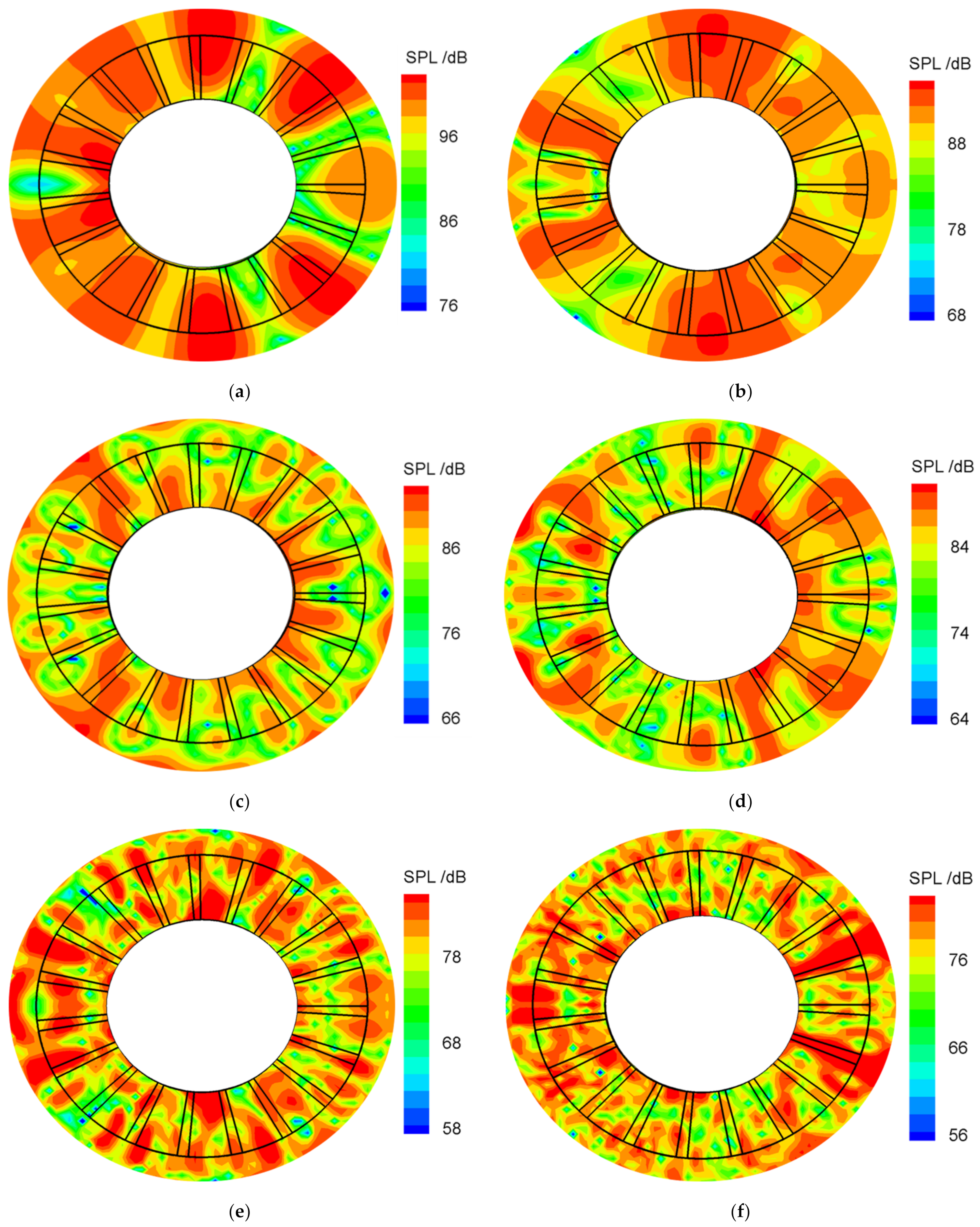
The radial resolution is very important to identify the spanwise distribution of a single blade sound source. Whether rotor blade or stator vane, determining how to quantify the noise sources on adjacent blades is required to improve the circumferential angle resolution in the process of source recognition as much as possible. For axial flow fans with high consistency consisting of multiple blades, it is important to improve the radial resolution to identify the spanwise noise source distribution of a single rotor/stator blade, especially to quantitatively evaluate the sound source intensity at blade root and tip. Moreover, due to the compact arrangement of blades, determining how to quantify the contribution of adjacent blades to noise radiation depends on the circumferential identification of sound sources. Figure 8 shows the reconstructed sound source maps evaluated for a one-third octave band from 2000 Hz to 6300 Hz at fan rotation with 49.6 Hz. The noise source maximum changes with increasing frequency, so the maps are displayed with different legends while the range of the color legend is always 26 dB. In the figure, the outer and inner black rings refer to the contour of the fan blade tip and the position where the blade root connects with the hub. Noise inside inner circles is hidden for convenience, this is because the region is not an actual physical noise source, but a by-product of possible reflections occurring during sound wave propagation. At low frequencies in Figure 8, between 2000 Hz and 2500 Hz, the noise source generated by each rotor blade cannot be effectively distinguished due to the large beamwidth allied to a few cut-on modes. In other words, the noise source appears more “blurred” around the blades. However, discrete noise sources above 2500 Hz are clearly shown around the tip area and fuzzy noise sources present in the hub region. At 3150 Hz, 4000 Hz, 5000 Hz, and 6300 Hz the sound source area of each blade is more obvious, and the noise contribution of each blade can be observed intuitively in the figure. Artificial output close to the hub walls also starts to become evident. It needs to be noted that these artifacts are not the actual noise sources, but the sound reflection from the duct wall and the obvious sidelobes caused by the microphone array itself, which is limited in size and installation position. These phenomena are consistent with the situation presented in Figure 5 and Figure 6. By comparing the source regions with the blade positions, the result appears good, knowing that: (a) the turbofan duct is annular, so there is no line of sight between each sound source and each microphone; (b) there is no liner between rotor and duct flush-mounted array. A distinctive feature of beamforming outputs is that the sound sources appear to be concentrated in the tip region rather than distributed along the span. This may mean that the sources appear in tip regions (e.g., tip vortices due to rotor blades) are of major importance. Note that the source position on the sound source map does not exactly match the desired source position under the mainlobe of the beamwidth at 2000 Hz and 2500 Hz due to the small number of modal waves cut-on in the flow duct at low frequencies. At higher frequencies, the source discriminability increases, followed by a reduction in sidelobe levels, thanks to the large number of cut-on modes that allow for better representation of source location. Overall, these visualizations validate the code. In this frequency band, the main sound source is located near the tip region. This is reasonable because the circumferential velocity increases from the hub to the tip, which results in a stronger interaction mechanism between the leading edge of the fan blade and the inflow flow [25]. Although there are no obstacles upstream, for fans, the sound source is expected to be in the leading edge region, as the inflow usually maintains some degree of turbulent intensity, even under free inflow conditions. In addition, tip leakage flow can lead to instability of the flow field in the tip region, especially for un-skewed fans, with greatly increased turbulence intensity levels [26].
5. Conclusions
An evaluation method of ducted rotating sources is presented. Based on this approach, the interpolated sound pressure due to the synchronized rotation of the virtual array and the modal steering vectors are generated coupled with the resampling processing of time series signals. By considering the influence of duct wall on acoustic wave propagation and the phase variation caused by source rotation, the data postprocessing embedded in this method allows the application of complex source characterization methods that are only suitable for fixed sources. Beamforming with the wall flush-mounted array exhibited noise sources appear to be concentrated in the tip region rather than distributed along the span. In other words, sources distributed along the fan seem to be of minor importance. The good quality of a wall flush-mounted array beamforming image is well understood while considering the presence of reflecting walls to generate the modal steering vector. Further research is needed to use a coaxially-mounted circular array with more microphones to investigate the detailed distribution of the sound field inside the flow duct.
Author Contributions
Conceptualization, K.X.; Formal analysis, K.X. and W.Q.; Investigation, W.Q. and Z.W.; Data curation, Y.S.; Funding acquisition, Z.W. All authors have read and agreed to the published version of the manuscript.
Funding
This work was supported by National Natural Science Foundation of China (Grant Nos.12002150), Ministry of Education (Grant No. 20YJCZH196), Natural Science Foundation of Jiangsu Province, China (Grant No. BK20201041).
Data Availability Statement
No new data were created or analyzed in this study. Data sharing is not applicable to this article.
Conflicts of Interest
The authors declare no conflict of interest.
Abbreviations
| sound source | |
| speed of sound | |
| acoustic sound pressure | |
| density of the flow | |
| frequency of interest | |
| emission time | |
| radial shape function of the (m, n) mode | |
| R | duct radius |
| n | radial mode order |
| t | time |
| Xm(t) | acoustic information |
| point spread function | |
| Green function | |
| intensity distribution of dipole source | |
| unit vector | |
| axial wave number of (m, n) mode | |
| m | circumferential mode order |
References
- Pannert, W.; Maier, C. Rotating beamforming–motion-compensation in the frequency domain and application of high-resolution beamforming algorithms. J. Sound Vib. 2013, 333, 1899–1912. [Google Scholar] [CrossRef]
- Herolda, G.; Sarradj, E. Microphone array method for the characterization of rotating sound sources in axial fans. Noise Control Eng. 2015, 63, 546–551. [Google Scholar] [CrossRef]
- Sijtsma, P. Feasibility of In-duct Beamforming. In Proceedings of the 13th AIAA/CEAS Aeroacoustics Conference, AIAA 2007-3696, Rome, Italy, 21–23 May 2022. [Google Scholar]
- Sijtsma, P. Using Phased Array Beamforming to Locate Broadband Noise Sources Inside a Turbofan Engine; NLR Report, NLR-TP-2009-689; National Aerospace Laboratory NLR: Amsterdam, The Netherlands, 2010. [Google Scholar]
- Sijtsma, P.; Oerlemans, S.; Holthusen, H. Location of Rotating Sources by Phased Array Measurements; NLR Report, NLR-TP-2001-135; National Aerospace Laboratory NLR: Amsterdam, The Netherlands, 2001. [Google Scholar]
- Minck, O.; Binder, N.; Cherrier, O.; Lamotte, L.; Pommier-Budinger, V. Fan noise analysis using a microphone array. In Proceedings of the Fan 2012-International Conference on Fan Noise, Technology, and Numerical Methods, FR, Senlis, France, 18–20 April 2012; pp. 1–9. [Google Scholar]
- Holland, K.R.; Nelson, P.A. An experimental comparison of the focused beamformer and the inverse method for the characterisation of acoustic sources in ideal and non-ideal acoustic environments. J. Sound Vib. 2012, 331, 4425–4437. [Google Scholar] [CrossRef]
- Brooks, T.F.; Humphreys, W.M., Jr. Deconvolution Approach for the Mapping of Acoustic Sources (DAMAS) determined from phased microphone arrays. In Proceedings of the 10th AIAA/CEAS Aeroacoustics Conference, Manchester, UK, 10–12 May 2004. [Google Scholar]
- Sijtsma, P. CLEAN Based on Spatial Source Coherence; NLR Report, NLR-TP-2007-345; National Aerospace Laboratory NLR: Amsterdam, The Netherlands, 2007. [Google Scholar]
- Sarradj, E. A fast signal subspace approach for the determination of absolute levels from phased microphone array measurements. J. Sound Vib. 2019, 329, 1553–1569. [Google Scholar] [CrossRef]
- Dougherty, R.P.; Ramachandran, R.C.; Raman, G. Deconvolution of sources in aeroacoustic images from phased microphone arrays using linear programming. Int. J. Aeroacoustics 2013, 12, 699–717. [Google Scholar] [CrossRef]
- Underbrink, J.R.; Dougherty, R.P. Array design for non-intrusive measurement of noise sources. Proc. Noise-Con 1996, 96, 10019651198. [Google Scholar]
- Dougherty, R.; Walker, B. Virtual rotating microphone imaging of broadband fan noise. In Proceedings of the 15th AIAA/CEAS Aeroacoustics Conference, AIAA 2009-3121, Miami, FL, USA, 11–13 May 2009. [Google Scholar]
- Lowis, C.R.; Joseph, P. A focused beamformer technique for separating rotor and stator-based broadband sources. In Proceedings of the 12th AIAA/CEAS Aeroacoustics Conference, AIAA-2006-2710, Cambridge, MA, USA, 8–10 May 2006. [Google Scholar]
- Lowis, C.R. In-Duct Measurement Techniques for the Characterisation of Broadband Aeroengine Noise. Ph.D. Thesis, University of Southampton, Southampton, UK, 2007. [Google Scholar]
- Poletti, M.A.; Teal, P.D. Comparison of methods for calculating the sound field due to a rotating monopole. J. Acoust. Soc. Am. 2011, 129, 3513–3520. [Google Scholar] [CrossRef] [PubMed]
- Poletti, M.A. Series expansion of rotating two and three dimensional sound fields. J. Acoust. Soc. Am. 2010, 128, 3513–3520. [Google Scholar] [CrossRef] [PubMed]
- Carley, M. Series expansion for the sound field of rotating sources. J. Acoust. Soc. Am. 2006, 120, 1252–1256. [Google Scholar] [CrossRef] [Green Version]
- Carley, M. Inversion of spinning sound fields. J. Acoust. Soc. Am. 2009, 125, 690–697. [Google Scholar] [CrossRef] [PubMed] [Green Version]
- Carley, M. Sound radiation from propellers in forward flight. J. Sound Vib. 1999, 225, 353–374. [Google Scholar] [CrossRef]
- Finez, A.; Leneveu, R.; Picard, C.; Leneveu, R.; Souchotte, P. In-Duct Acoustic Source Detection Using Acoustic Imaging Techniques. In Proceedings of the 19th AIAA/CEAS Aeroacoustics Conference, Berlin, Germany, 27–29 May 2013. [Google Scholar]
- Gérard, A.; Berry, A.; Masson, P. Control of tonal noise from subsonic axial fan, Part 1. J. Sound Vib. 2015, 288, 1049–1075. [Google Scholar] [CrossRef]
- Caldas, L.C.; Greco, P.C.; Pagani, C.C.; Baccalá, L.A. Comparison of different techniques for rotating beamforming at the University of São Paulo fan rig test facility. In Proceedings of the 6th Berlin Beamforming Conference, BeBeC-2016-D14, Berlin Germany, 24–25 February 2016. [Google Scholar]
- Johnson, D.H.; Dudgeon, D.E. Array Signal Processing: Concepts and Techniques; Prentice Hall: Hoboken, NJ, USA, 1993. [Google Scholar]
- Krömer, F.; Müller, J.; Becker, S. Investigation of aeroacoustic properties of low-pressure axial fans with different blade stacking. AIAA J. 2018, 56, 1507–1518. [Google Scholar] [CrossRef]
- Zhu, T.; Lallier-Daniels, D.; Sanjosé, M.; Moreau, S.; Carolus, T. Rotating coherent flow structures as a source for narrowband tip clearance noise from axial fans. J. Sound Vib. 2018, 417, 198–215. [Google Scholar] [CrossRef]
Figure 1.
Noise radiation from rotating dipole sound sources in infinitely long duct.

Figure 2.
Schematic diagram of fan experimental test with an anechoic termination outlet duct.

Figure 3.
Inlet noise measuring section in semi-anechoic chamber and photo of axial flow fan.

Figure 4.
Modal cut-on function spectrum of single-stage fan. (a) Modal cut-on function. (b) Radial modes of mode order m.
Figure 4.
Modal cut-on function spectrum of single-stage fan. (a) Modal cut-on function. (b) Radial modes of mode order m.
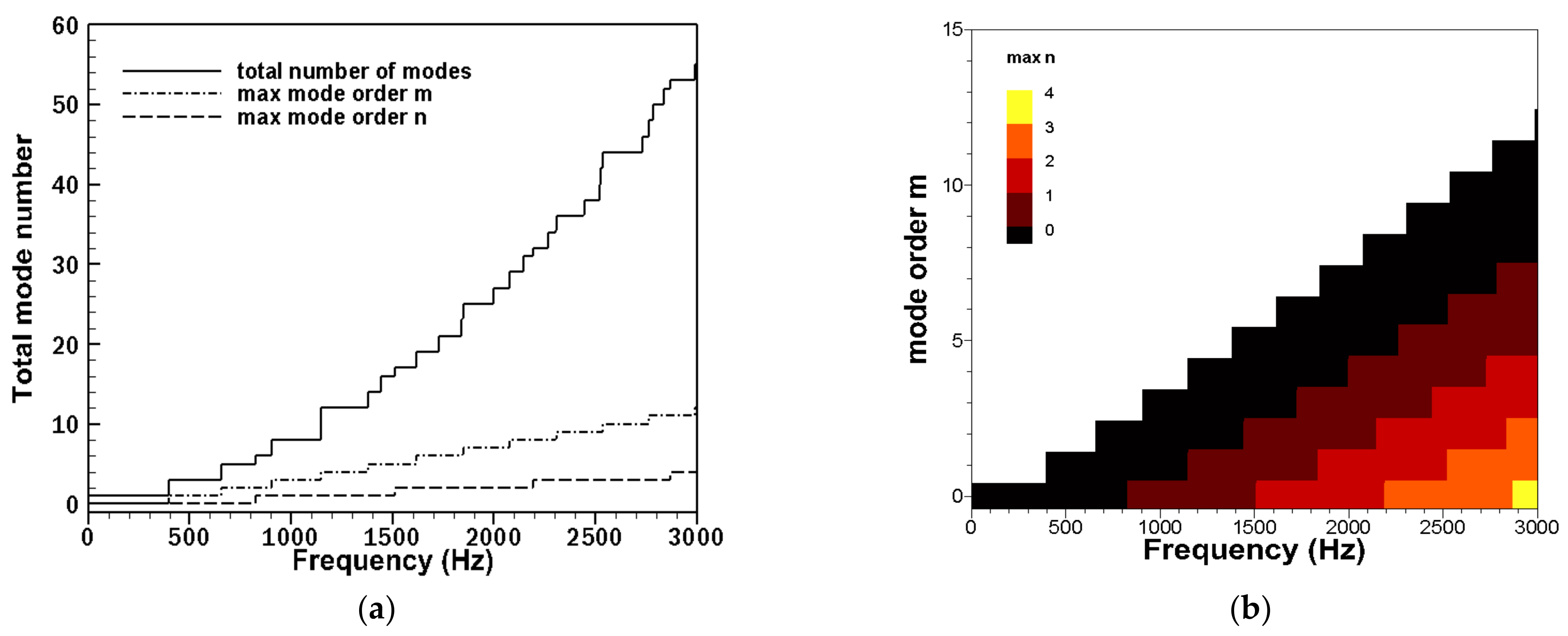
Figure 5.
Conventional beamforming coupled with virtual rotating array for three sources at R = 0.3 m and angles are 0, 0.5 , 1.0 , processing frequency = 3000 Hz, rotating frequency = 49.6 Hz. (a) 0 s; (b) 0.15s; (c) 0.3 s; (d) 0.45 s; (e) 0.6 s; (f) 0.75 s; (g) 0.9 s; (h) 1.05 s; (i) 1.2 s.
Figure 5.
Conventional beamforming coupled with virtual rotating array for three sources at R = 0.3 m and angles are 0, 0.5 , 1.0 , processing frequency = 3000 Hz, rotating frequency = 49.6 Hz. (a) 0 s; (b) 0.15s; (c) 0.3 s; (d) 0.45 s; (e) 0.6 s; (f) 0.75 s; (g) 0.9 s; (h) 1.05 s; (i) 1.2 s.
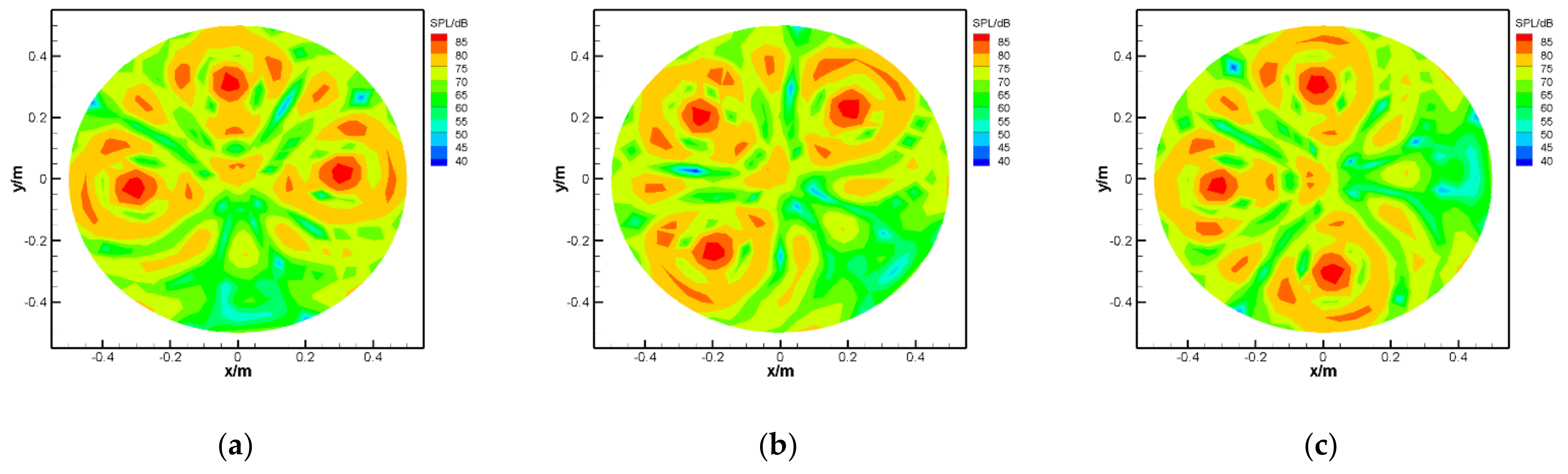

Figure 6.
Sound maps of three rotating sources simulation. (a) Conventional beamforming; (b) Clean-SC method; (c) DAMAS method.
Figure 6.
Sound maps of three rotating sources simulation. (a) Conventional beamforming; (b) Clean-SC method; (c) DAMAS method.

Figure 7.
Noise source map in axial flow fan at 3150 Hz: (a) using free-field Green function to generate steering vector; (b) using ducted Green function to generate steering vector; (c) using ducted Green function to generate steering vector with resampling process.
Figure 7.
Noise source map in axial flow fan at 3150 Hz: (a) using free-field Green function to generate steering vector; (b) using ducted Green function to generate steering vector; (c) using ducted Green function to generate steering vector with resampling process.

Figure 8.
Sound source maps for an axial fan for eight different frequencies between 2000 Hz and 6300 Hz. (a) 2000 Hz; (b) 2500 Hz; (c) 3150 Hz; (d) 4000 Hz; (e) 5000 Hz; (f) 6300 Hz.
Figure 8.
Sound source maps for an axial fan for eight different frequencies between 2000 Hz and 6300 Hz. (a) 2000 Hz; (b) 2500 Hz; (c) 3150 Hz; (d) 4000 Hz; (e) 5000 Hz; (f) 6300 Hz.
Publisher’s Note: MDPI stays neutral with regard to jurisdictional claims in published maps and institutional affiliations. |
© 2022 by the authors. Licensee MDPI, Basel, Switzerland. This article is an open access article distributed under the terms and conditions of the Creative Commons Attribution (CC BY) license (https://creativecommons.org/licenses/by/4.0/).
Share and Cite
MDPI and ACS Style
Xu, K.; Shi, Y.; Qiao, W.; Wang, Z. The Methodological and Experimental Research on the Identification and Localization of Turbomachinery Rotating Sound Source. Energies 2022, 15, 8647. https://doi.org/10.3390/en15228647
AMA Style
Xu K, Shi Y, Qiao W, Wang Z. The Methodological and Experimental Research on the Identification and Localization of Turbomachinery Rotating Sound Source. Energies. 2022; 15(22):8647. https://doi.org/10.3390/en15228647
Chicago/Turabian StyleXu, Kunbo, Yun Shi, Weiyang Qiao, and Zhirong Wang. 2022. "The Methodological and Experimental Research on the Identification and Localization of Turbomachinery Rotating Sound Source" Energies 15, no. 22: 8647. https://doi.org/10.3390/en15228647
Note that from the first issue of 2016, this journal uses article numbers instead of page numbers. See further details here.