
A Filter-Less Time-Domain Method for Reference Signal Extraction in Shunt Active Power Filters


1
ECE Department, Faculty of Engineering, Beirut Arab University, Beirut 11-5020, Lebanon
2
LaRGES, CRSI, Faculty of Engineering, Lebanese University, Tripoli 1300, Lebanon
3
College of Engineering and Technology, American University of the Middle East, Kuwait
*
Author to whom correspondence should be addressed.
Energies 2022, 15(15), 5568; https://doi.org/10.3390/en15155568
Submission received: 7 July 2022
/
Revised: 21 July 2022
/
Accepted: 28 July 2022
/
Published: 31 July 2022
(This article belongs to the Special Issue Active Power Filters and Power Quality)
Abstract
:Current distortion degrades power quality and affects system performance, especially for sensitive loads that require pure sinusoidal waves. Owing to its excellent dynamic response, a well-designed active power filter (APF) can achieve a total harmonic distortion (THD) within the acceptable limits defined by IEEE 3002 standards through compensating harmonic distortions. The APF consists of two main modules: a reference signal extraction module and a modulation module. This paper adapts the matrix pencil method, a well-known model-based parameter estimation technique, to the problem of reference extraction. Contrary to conventional time-domain methods such as the synchronous reference frame (SRF) and the reactive power theory (PQ theory) that rely on low-pass filters in their implementations, the proposed method does not use a filter. However, it extracts the reference signal by first decomposing the load current into its constituent frequency components, and then subtracting the pure sine wave synthesized from the obtained fundamental component from the load current. Results on simulated data from MATLAB/Simulink confirm the higher accuracy and fast response time of the proposed method in extracting the reference signal.
1. Introduction
Nowadays, the widespread usage of nonlinear loads in households and industries is affecting power quality. Loads ranging from small personal appliances and devices such as laptops, chargers, and LED lights, to industrial equipment such as arc furnaces, variable-frequency drives, variable-speed motors drives, and railway systems [1,2] all result in voltage and current harmonic distortions on the grid. If not compensated, these harmonics may have many negative effects on the power system as they can contribute to voltage drop, an increase in losses, overheating of power equipment and higher neutral currents which may lead to insulation failure and breakdown. Most of the power equipment can, to some extent, withstand poor power quality. However, modern equipment that is electronically controlled, either through power conversions such as DC and AC drives or through peripheral controls such as programmable logic controllers and microprocessor controllers, are more sensitive to harmonic distortions [3]. This has raised the issue of power quality among consumers who are increasingly concerned about the power quality they are receiving from the power companies [4].
An active power filter (APF), owing to its dynamic response and reliability, constitutes a viable solution for harmonic compensation. It is designed to eliminate harmonics, correct power factor, and balance AC power networks. These filters are referred to as active since they have a dynamic response to the change of load, unlike passive filters designed to compensate for specific harmonics at a specific load [5]. Although active filters are more expensive, their load variation response guarantees to a certain extent the achievement of the total harmonic distortion (THD) level within the IEEE required level. A shunt APF eliminates the harmonics of the source current by injecting an opposite and equal compensating current [6]. Since reference signal extraction is the first module of the active power filter, accurate and fast extraction of the reference has an impact on the overall performance of the filter. Two of the most used time-domain methods for reference signal extraction in active power filters are the synchronous reference frame (SRF) and the instantaneous reactive power theory (PQ). A main advantage of these methods is their simple implementation [7,8]. However, they involve a low-pass filter in their implementation, which can cause large amplitude and phase errors and, as a result, can lead to poor harmonic compensation [9,10].
In this paper, a model-based parameter estimation method called the matrix pencil method (MPM) is proposed for the problem of reference signal extraction in the time domain without using a filter. Assuming the non-linear load current can be expressed as a linear combination of sinusoidal signals, the MPM estimates the amplitude and frequency of each frequency component in the load current. This decomposition of the load current into its constituent frequency components enables synthesizing the pure sine wave of the fundamental component, which is then subtracted from the load current to obtain the reference signal. In comparison with the SRF and PQ methods, the MPM achieves higher accuracy and a faster response time.
The rest of the paper is organized as follows. Section 2 gives the structure of the shunt active power filter simulated in this paper. Section 3 reviews the theory behind the SRF and PQ methods. In Section 4, the signal model of the current drawn by the nonlinear load and the steps of the proposed method are given. Section 5 evaluates the performance of the proposed method in terms of accuracy and response time. Finally, Section 6 draws the conclusions of this work.
2. Shunt Active Power Filter (SAPF) Structure
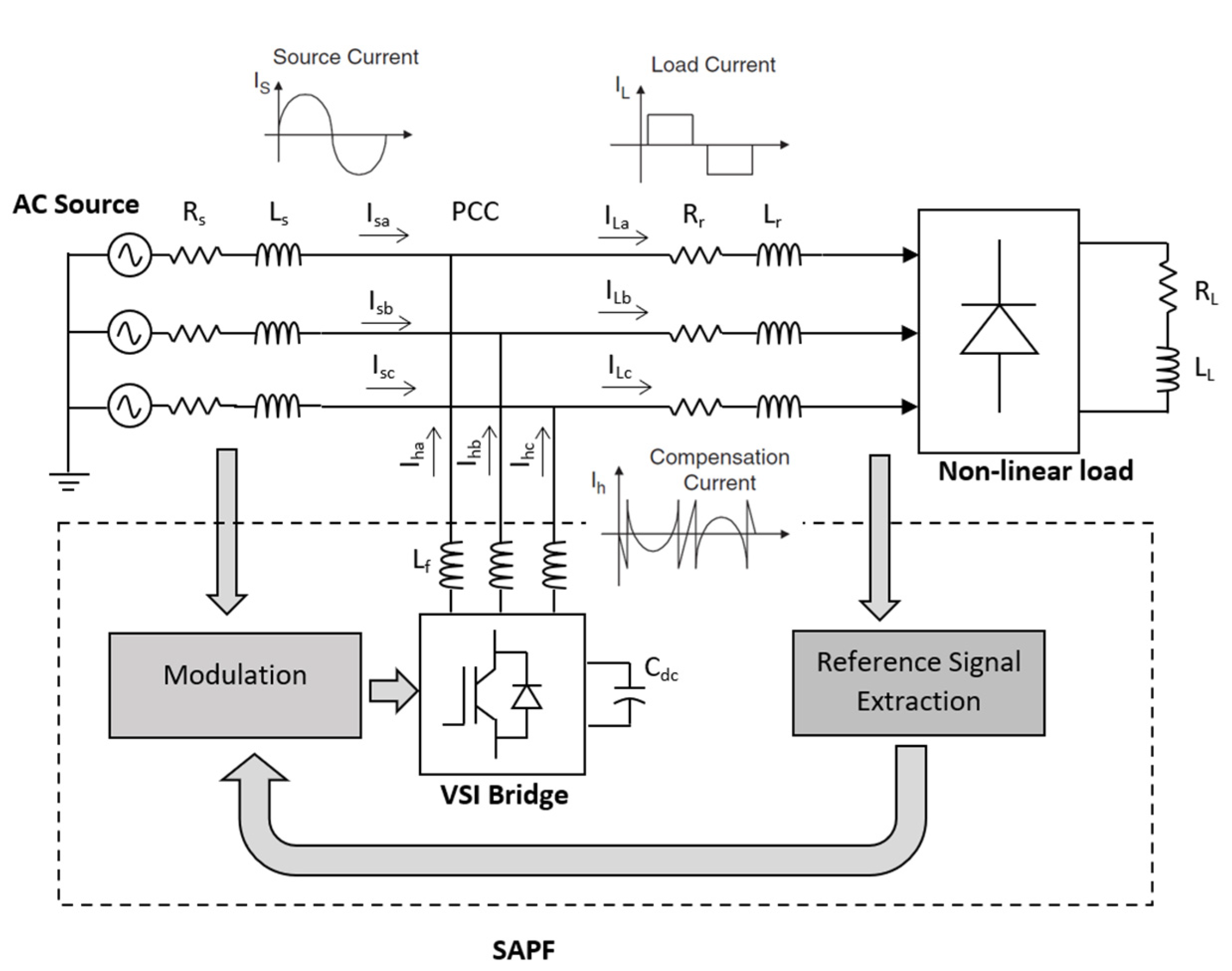
SAPF as a circuit structure consists of a voltage source inverter (VSI) with a modulation process, and a reference signal extraction process as shown in Figure 1. The modulation process, which is commonly known as the pulse width modulation (PWM), enables the DC voltage source to be converted into AC and injected into the system for harmonic elimination. Other modulation processes are also used, such as the hysteresis control and the space vector modulation. The physical structure of the active filter is mature in principle. However, the two main parts, including the extraction of the reference signal and the modulation process, are still under improvement to achieve a lower THD of the source current, a faster response of the source current in reaching a constant THD, and an increased efficiency [5].
The power circuit of the SAPF consists of a three phase AC source with source impedance (Rs, Ls), supplying a non-linear load which consists of a full bridge rectifier containing load (RL, LL) through a line impedance (Rr, Lr). The VSI DC link containing capacitor (Cdc), with its modulation control and reference signal extraction process, forms the SAPF which is connected to the power circuit at the point of common coupling (PCC) through a coupling reactance (Lf). Isa, Isb, and Isc represent the mains source currents. ILa, ILb, and ILc represent the load currents. Iha, Ihb, and Ihc represent the compensated injected currents to the power system. The SAPF works by injecting the compensating currents, which are equal but opposite harmonics currents at the PCC. This results in eliminating the load harmonic currents and, consequently, making the source current sinusoidal.
3. Commonly Used Signal Extraction Methods
Accurate reference signal extraction is essential for a high-performance system with minimum source current harmonic distortion, since it forms the controlling signal of the VSI switches. Its estimation depends on system variables and can be computed in time and frequency domains [11]. The most used extraction techniques are the PQ theory and the synchronous reference frame theory. Some recent developments of these techniques can be found in [12,13,14].
3.1. Synchronous Reference Frame Theory
In three-phase three-wire systems, the SRF harmonic extraction technique is widely used as the simplest and most easily implemented technique. In comparison to the p-q theory, the SRF approach provides the best compensation output because it is insensitive to voltage disturbances. The load current signal is converted into a synchronous reference frame. The AC mains voltage is used to synchronize the reference frame. The synchronization control has many techniques as described in [15,16]. The SRF could be derived as per the below equations, considering a symmetrical balanced system and hence neglecting the zero sequence components:
where p and q represent the total active and reactive powers, and are the currents in the alpha-beta frame, and and are the currents in d-q frame.
The angle between id and iq is 90 degrees, and that between the α axis and id is (rotation angle) which is attained using the phase locked loop (PLL). Then:
From the above equations, the active and reactive power depends on the id and iq.
The d-q currents are calculated by means of the following equation:
and
where is the DC component of corresponding to the only desired power (active power) is the AC component, and are the DC and the AC components of . The , and need to be eliminated by the use of the low pass filter, so the required d and q currents will be and :
This algorithm enables calculation of the reference frame currents directly from the load current without the usage of mains voltages. As a result, mains voltage distortion or unbalance does not affect the reference compensating currents. To generate theta of the Clarke transformation, a PLL is required.
3.2. Instantaneous Reactive Power Theory
The PQ theory is considered the most widely used extraction method in the APF due to its fast response and acceptable THD. Akagi in [17] started developing the control strategies considering both transient and steady-state efficiency.
This procedure is derived based on the Clarke transformation, and the required compensation current is then calculated using the two-axis technique. The p-q approach is then used to convert mains current and voltage into two-axis representations. The instantaneous actual power and instantaneous imaginary power consumed by the loads are then computed. These control components receive reference compensating currents. The reference compensated currents are calculated using inverse transformation; the reference currents are then obtained.
First, the three-phase load currents source voltages are used to get the equivalent currents in an alpha-beta frame using Clarke power transformation:
Then the active and reactive powers are calculated using the following equation:
Inversing the above matrix equation, we get:
Then expanding it we get:
where:
Expanding the above equation further we get:
where:
This equation demonstrates the whole theory that load currents on the alpha-beta axis are composed of four powers:
The instantaneous total active current and total reactive currents are p and q, respectively. The total power, either p or q, is divided into a DC component and an AC component. The DC component relative to instantaneous power p is , which is the desired power component to be supplied by the power source. The AC component of the instantaneous power p is , related to the harmonic current. The DC component of the imaginary instantaneous power q is and is associated with the reactive power. The AC component of the imaginary instantaneous power q is , associated with the harmonic current [18]. The current mitigation could be achieved by calculating the value of the undesired powers and reinjecting them negatively at the coupling point. The only desired power is the DC component of p: .
To mitigate the reactive power and current harmonics, the reference extracted signal of the APF must include the values of and . Hence the required currents are:
where:
We then do an inverse Park transformation to obtain the filter/controller currents:
The PQ theory and SRF are two different approaches used for the extraction of the reference signal (harmonics) that is injected into the coupling point to mitigate the current harmonics drawn from the supply source. These methods were modified and optimized in [19].
4. The Proposed Signal Extraction Method
4.1. Signal Model
For a sinusoidal source voltage, the current flowing in a nonlinear load can be modeled by virtue of Euler’s formula as a summation of cisoids (complex-valued sinusoidal signals) weighted by complex residues according to the following damped exponential signal model [20]:
where is the complex residue of the cisoid and is its frequency. After sampling, the time variable, , is replaced by , where is the sampling period and is the sample index. The discrete current signal becomes:
where is the complex pole and N is the number of samples. Under matrix form, the signal model is expressed by:
where
The superscript denotes the transpose operator.
The problem of extracting the reference signal can now be stated as follows. Given the load current data sequence , we can estimate the amplitudes and the frequencies . The estimated parameters of the fundamental frequency are then used to construct the fundamental component of the nonlinear load current, i.e., a pure sine wave. This sine wave is subtracted from the load current to obtain the reference signal.
4.2. The Matrix Pencil Method
This section details the steps of the matrix pencil method (MPM), which is a model-based high-resolution algorithm. MPM exploits the matrix pencil structure of the underlying signals to estimate the parameters of the damped/undamped exponential model. It has been successfully used for parameter estimation in dispersive media [21,22,23], direction-of-arrival estimation [24], extraction of wave objects from scattering data [25], and frequency-dependent multi-path resolving [26]. In this work, the amplitudes and frequencies estimated by the MPM from the nonlinear load current will be used to construct the reference signal of the active power filter.
The following steps summarize the principle of the MPM.
- Step 1. Select the pencil parameter, , so that The proper choice of makes the MPM robust against noise.
- Step 2. Using the current data sequence , construct a Hankel data matrix:
- Step 3. Remove the first and last columns of to obtain the following two matrices, which in MATLAB notation are given by:
- Step 4. Use and to form a matrix pencil defined as , with a scalar parameter. In the case of a noiseless exponential data model, and admit the following Vandermonde decomposition [23]:andwhere
The Vandermonde decomposition reveals the shift-invariance property along the column and row spaces, and allows writing the matrix pencil as e:
- Step 5. Estimate the complex poles as the generalized eigenvalues of the matrix pair . The frequencies can then be estimated from the poles.
- Step 6. Estimate the amplitudes using a least-squares fit with the following solution: where the superscript denotes the conjugate-transpose operator.
5. Simulation Results and Discussion
To check the effectiveness of the MPM in active power filter applications, a comparison is done with the PQ and the SRF methods for two different systems: a reduced system and a complete system. The parameters used in the simulation are shown in Table 1. For the reduced system, only the reference signal extraction module of the SAPF shown in Figure 1 is simulated, while the modulation module, the DC-link capacitor, and the coupling inductance are not considered. Under these conditions, the source current is determined by directly subtracting the extracted reference signal from the load current without having to undergo any modulation or switching. The rationale behind using a reduced system is to isolate any contribution to the current THD other than that of the extraction method.
As for the complete system, both the extraction and modulation modules are considered, including the DC-link capacitor, the coupling inductor, a PWM for the modulation process, and a proportional integrator (PI) controller to maintain the DC-link capacitor at the desired reference voltage value. This system represents a practical SAPF and has the purpose of evaluating the performance MPM in a more realistic setting.
5.1. Reduced System
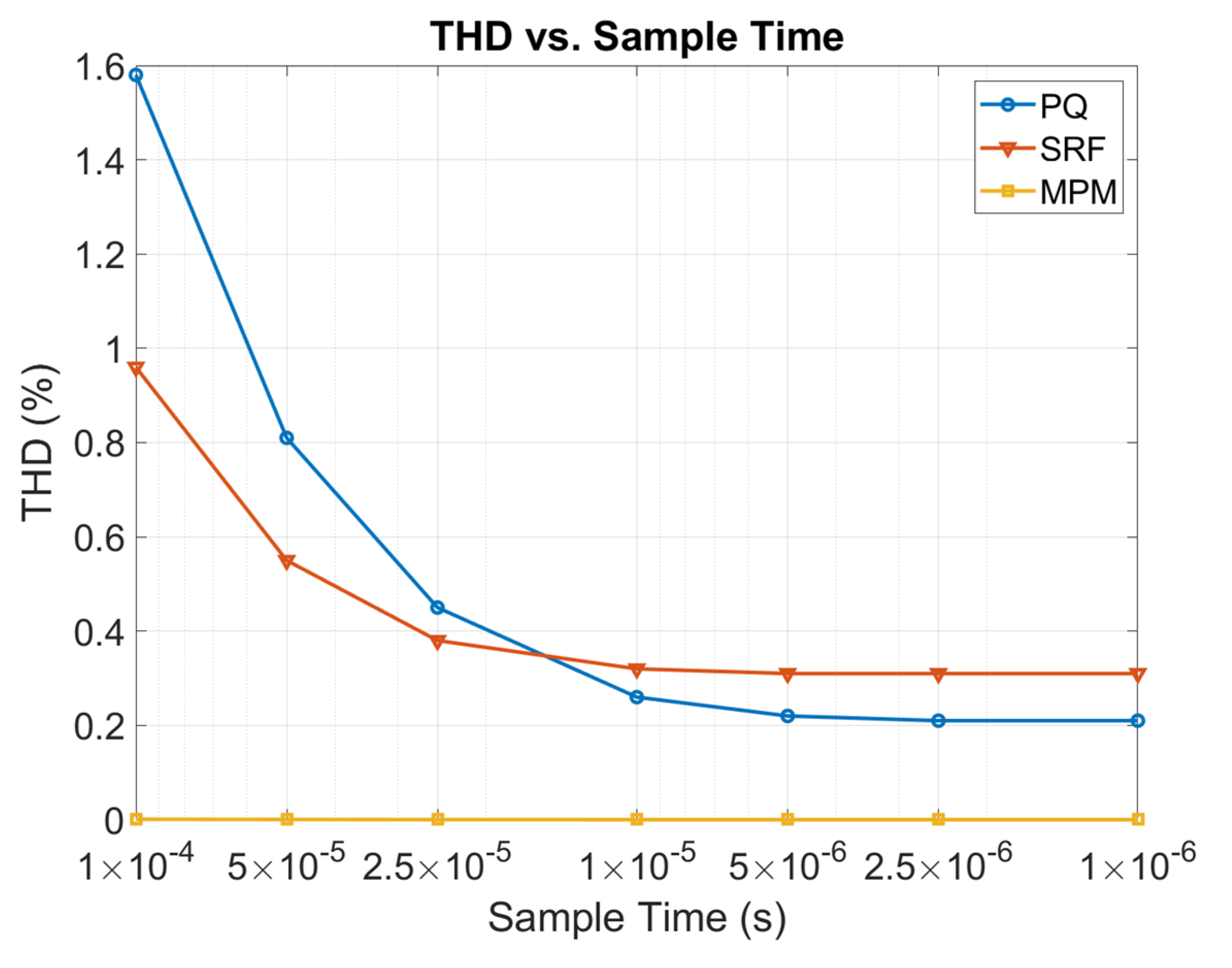
In this system, the harmonic compensation performance is evaluated with respect to accuracy which is the source current THD value and the response time. For the THD comparison, seven discrete time simulations are performed. Each one has a different time step, which is denoted as the simulation sample time starting from 1 × 10⁻⁴ s until 1 × 10⁻⁶ s as shown in Figure 2. The signal extraction accuracy at the steady state condition is undertaken by measuring the source current THD (%) at the different simulation sample times, to examine the effect of the discrete simulation time step change. The signal extraction response time evaluation is addressed by measuring the THD (%) in a transient state at a specific selected sample time (5 × 10⁻⁵ s) for the PQ, SRF, and MPM extraction methods.
The source current THD with no filter is 25.61%, which is higher than the 5% required by IEEE 3002 standards [27]. The APF is designed to maintain the source current THD less than 5%. The THD value that remains after installing the APF is due to modulation process errors and the signal extraction process errors. To identify the THD resulting from the signal extraction itself, independently from the THD resulting from the modulation process, the load current containing the harmonics is subtracted from the extracted reference signal to represent the source current after harmonic mitigation. The THD measured represents the error of the signal extraction method itself, regardless of the modulation process.
The system is simulated seven times using a discrete simulation type, each at different sample time steps representing the extraction methods performance. The steady state source current THD (%) for each extraction method is measured in each simulation and is represented in Figure 3. The PQ and SRF performance depend on the sample time step; the THD decreases when the sample time step decreases. The PQ reaches its best THD of 0.21% at 2.5 × 10⁻⁶ s sample time, and the SRF reaches its best THD of 0.31% at 5 × 10⁻⁶ s sample time. As for the MPM, the results reveal that it is independent of the sample time change and has a THD of 1.49 × 10⁻⁶%, which is almost zero in the reduced system. These results are represented in Figure 2. Therefore, the MPM gives a more accurate and better performance in reference signal extraction. It overcomes the phase and magnitude errors in reference signal extraction due to the presence of the low pass filter in PQ and SRF. Moreover, it is not affected when changing the discrete simulation time step, unlike the PQ and SRF which has higher source current % THD with a larger time step.
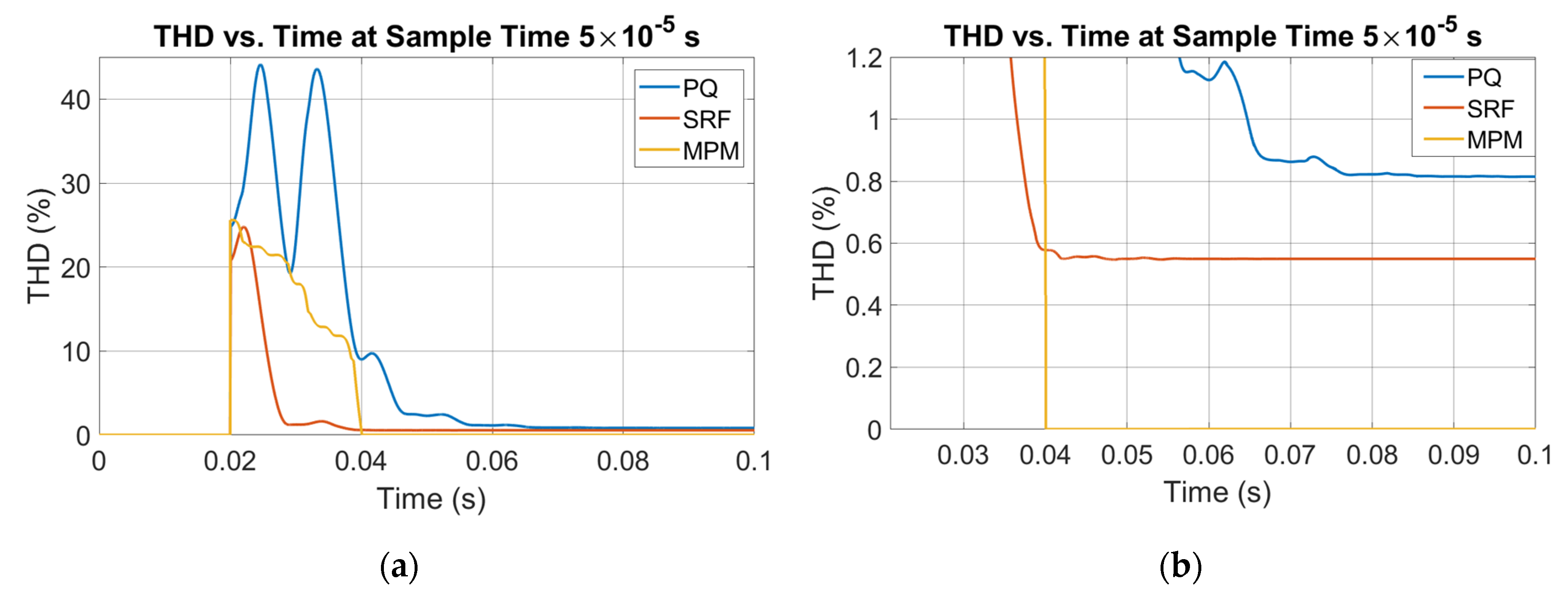
As for the transient response, Figure 3 shows the THD measurements for the three methods with respect to time at a specific sample time step of 5 × 10⁻⁵ s. Having the source frequency of 50 Hz, the first 0.02 s represent the first cycle, which is the minimum time needed for calculating the THD. Hence the time span from 0 to 0.02 s does not represent any THD calculations.
The results show the first cycle THD which is calculated at time 0.02 s starts from a value near 25.61% for all the three methods. This represents the value of the source current THD without SAPF. The second cycle THD is measured at 0.04 s and shows that the three methods reach a THD value less than that with no filter. The PQ reaches the steady state of 0.81% THD at 0.095 s, the SRF reaches the steady state of 0.55% THD at 0.055 s, whereas the MPM reaches steady state THD of almost zero at 0.04 s. The results confirm the faster response of the MPM compared with the PQ and SRF when a reduced system is considered.
5.2. Complete System
After achieving a better performance and a faster response of the MPM in the reduced system over the PQ and SRF, the proposed method is evaluated for a complete practical SAPF. The complete system includes a DC-link capacitor and a coupling inductor and uses a PWM modulation at 12.5 kHz switching frequency. The sample time step of the discrete simulation is set to 1 × 10⁻⁶ s.
5.2.1. Static Response
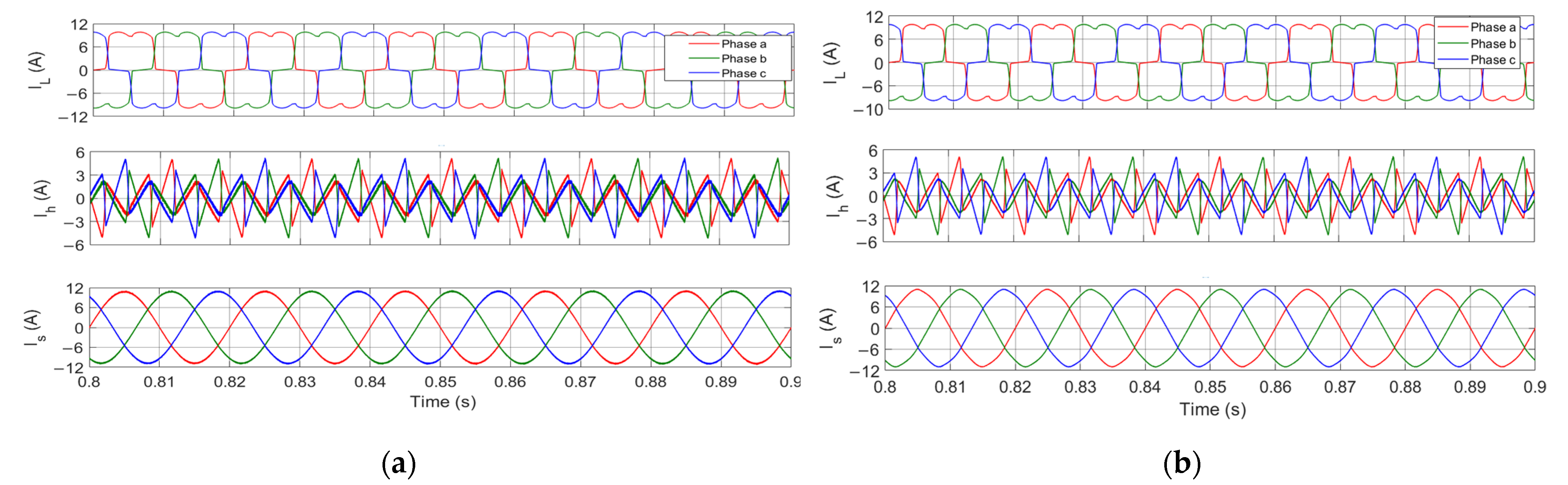
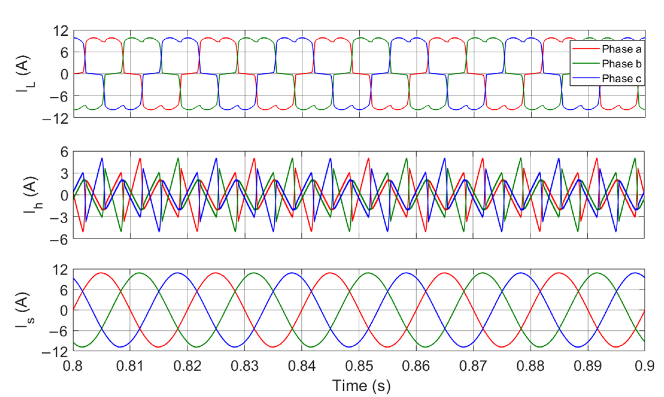
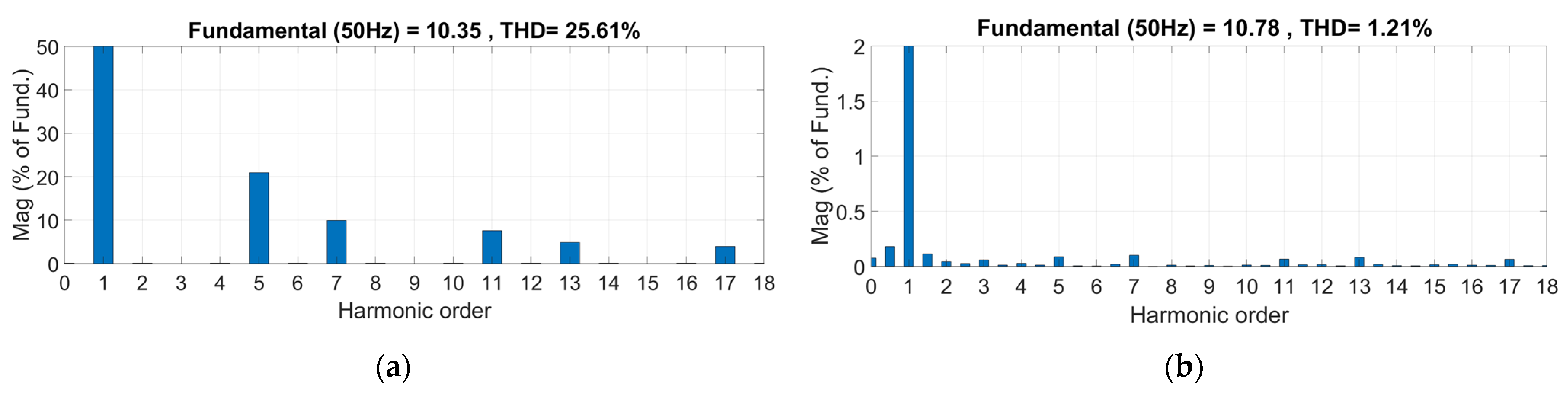
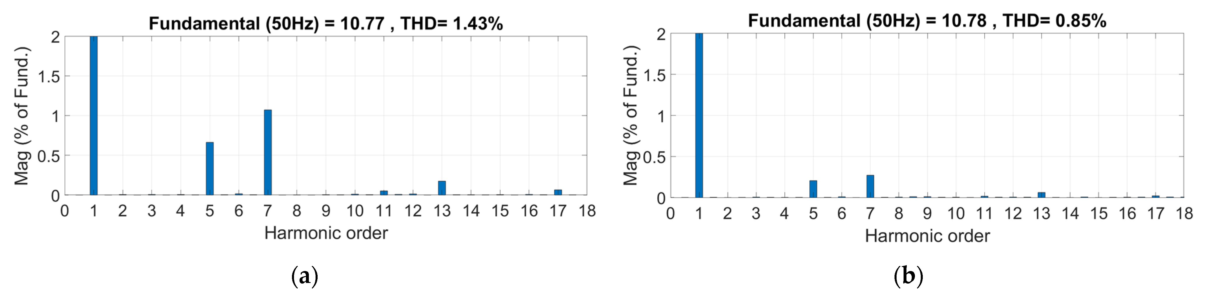
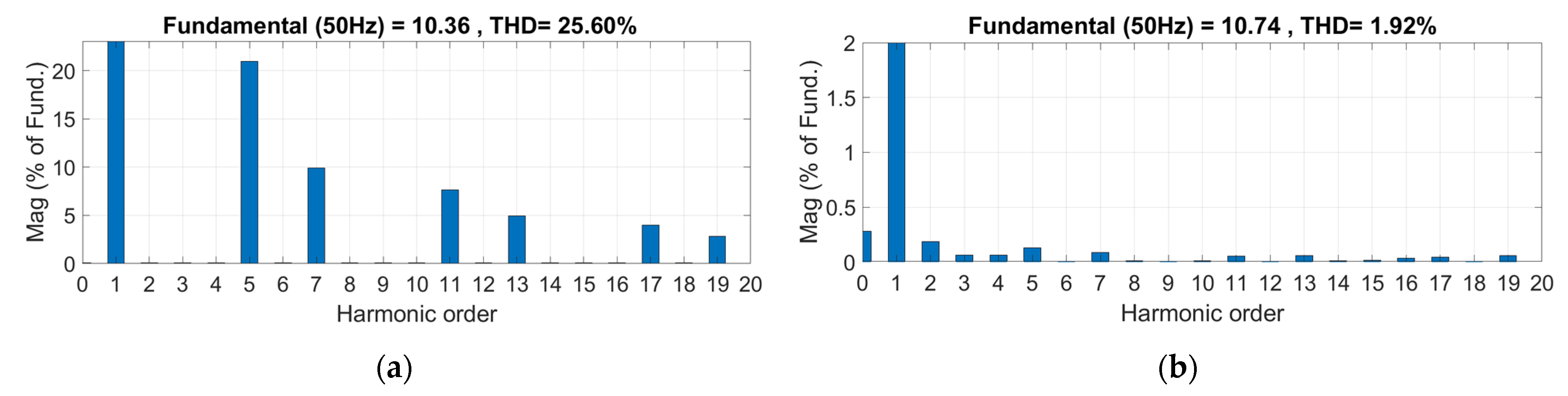
The fast Fourier transform (FFT) analysis of the source current without APF shows a THD of 25.61%. To reduce the power system harmonic distortion, the harmonics are compensated by injecting the mitigation current at the PCC. Figure 4 and Figure 5 represent the steady state waveforms of SAPF when using the PQ, SRF, and MPM. Each of the figures include the load current IL, the harmonics reference signal extracted Ih, and the source current Is. From the figures, it can be seen that all three methods succeed in compensating current harmonics and restoring the sinusoidal waveform of the source current. However, a closer look with the FFT analyzer in Figure 6 and Figure 7 shows that that MPM has a better performance, since it effectively reduces the 25.61% THD of the source current to 0.85%, whereas the PQ and SRF reduce it from 25.61% to 1.21% and 1.43%, respectively. The results are summarized in Table 2.
5.2.2. Response Time
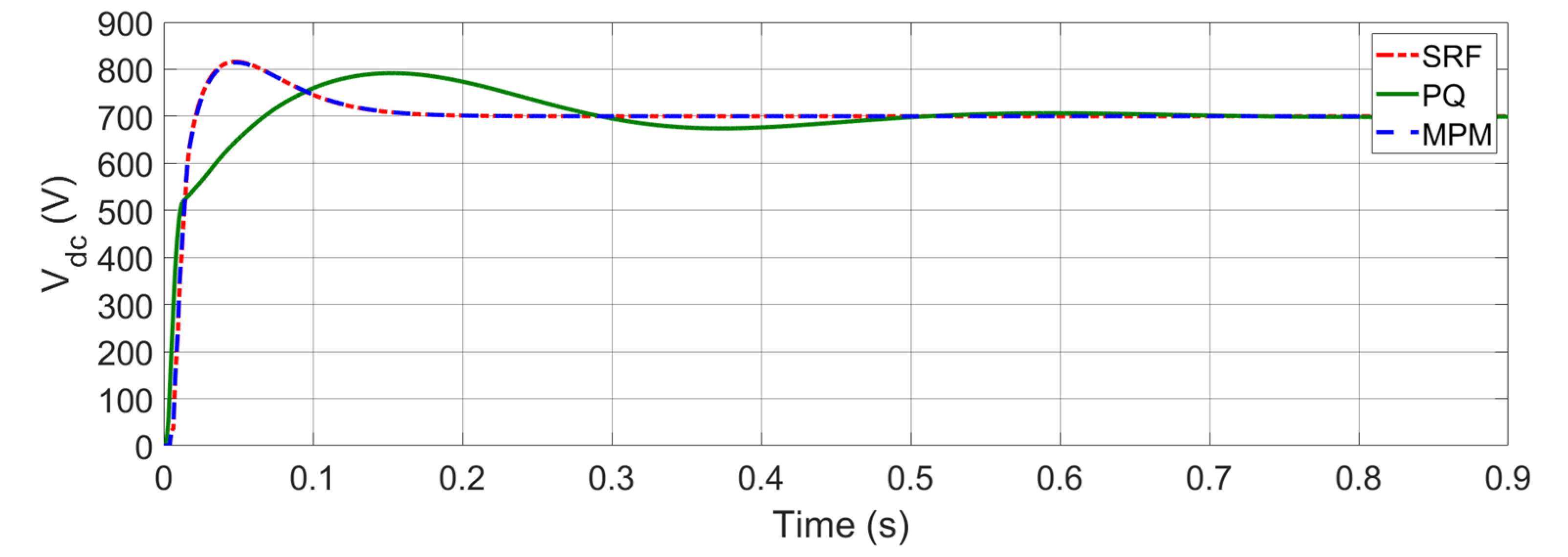
To check the response time of the MPM in a practical complete system, the capacitor voltage is measured in the transient state and the response time, which is the time needed for the capacitor voltage to reach its reference value of 700 V, is observed. Figure 8 represents the DC-link capacitor voltage value using the PQ, SRF, and MPM. The figure shows that the system takes around 0.8 s to reach its steady state when using the PQ, and approximately 0.2 s when using the SRF or MPM. Therefore, the MPM achieves a faster response than the PQ and almost the same response time as the SRF.
5.2.3. Dynamic Response
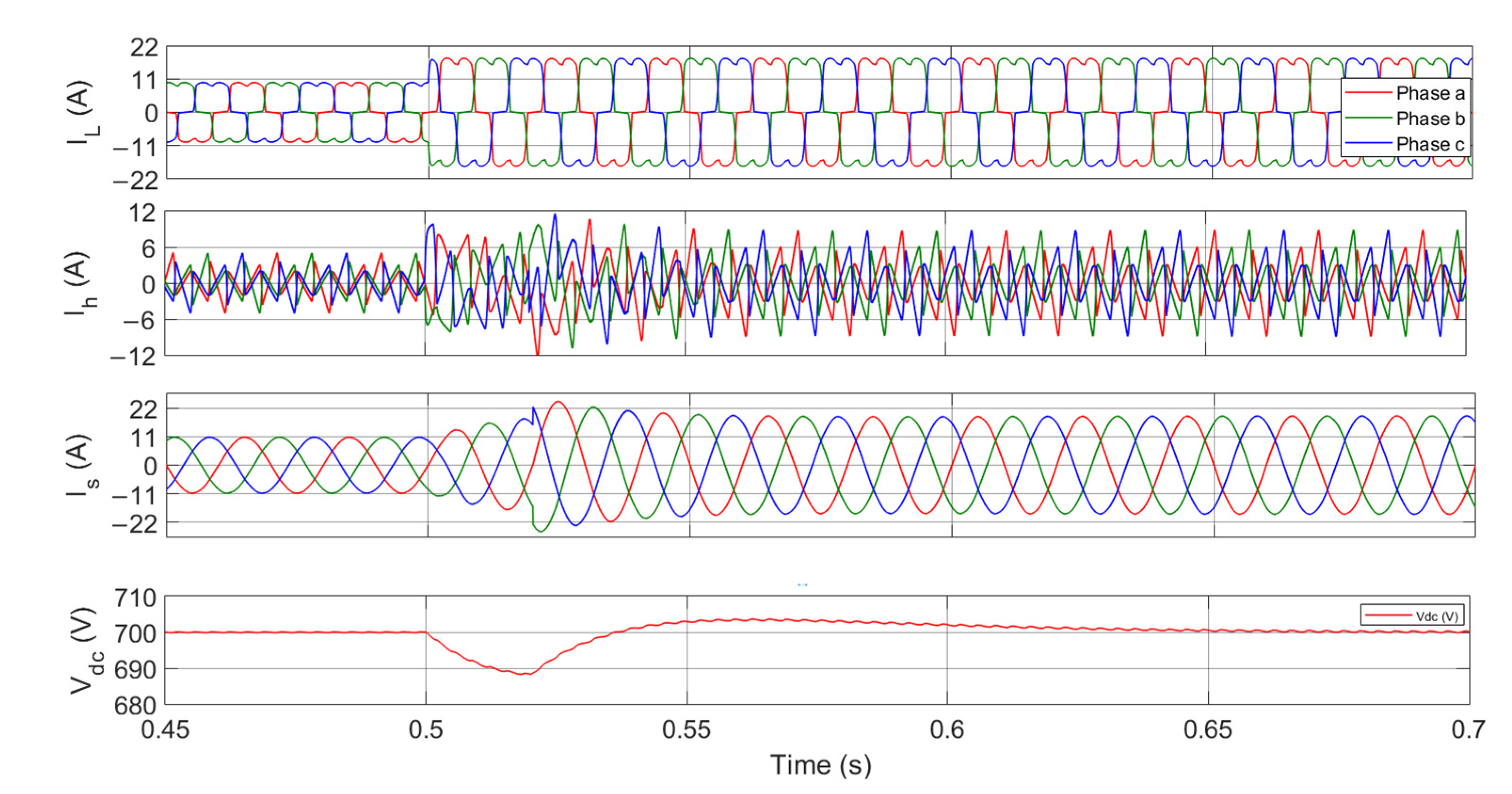
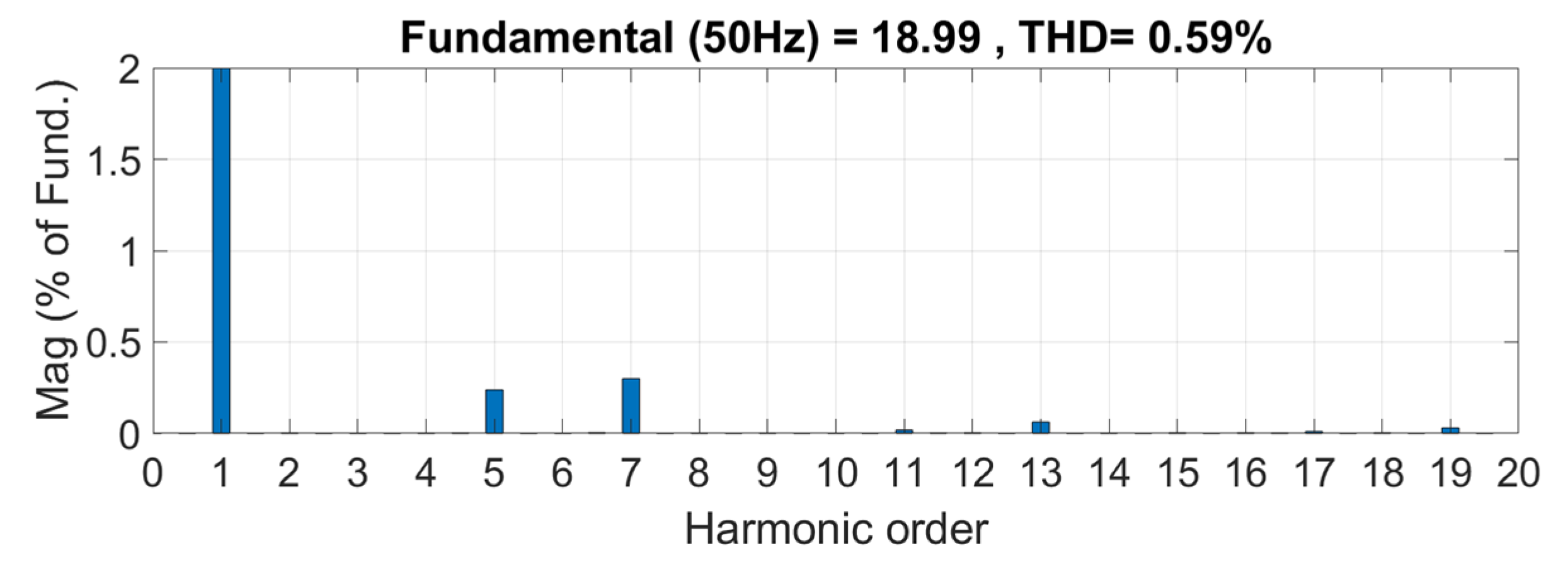
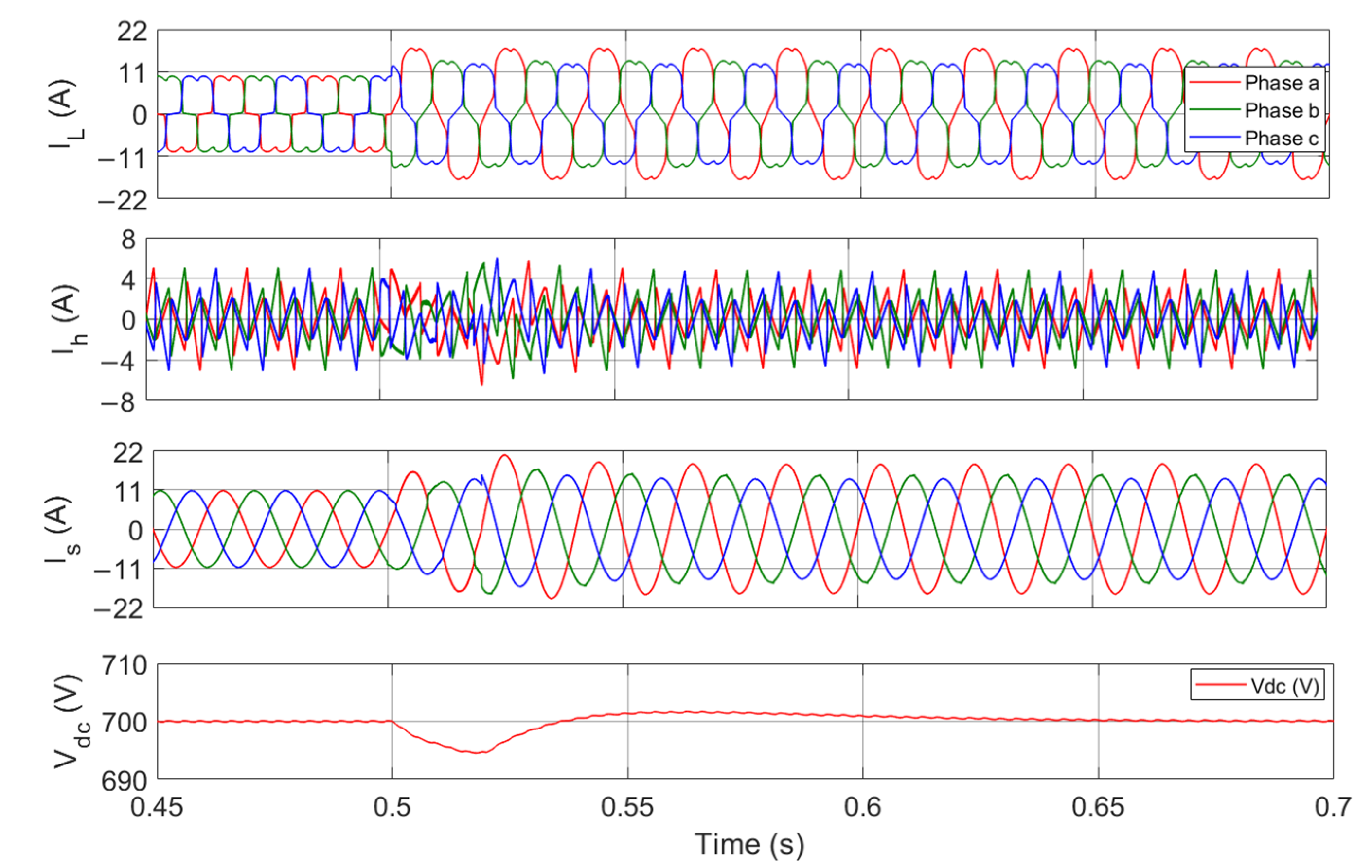
To study the MPM dynamic response during load variation, a transient-state condition is created by changing the resistance of the non-linear load RL from 40 Ω to 20 Ω at t = 0.5 s. The load current, harmonic current, and source current waveforms, in addition to the DC-link voltage, are shown in Figure 9. This shows the transient response of the APF in compensating the source harmonics under load change when using the MPM. The results in Figure 10 show a THD of 0.59% and thus the ability of the MPM to compensate current harmonics under dynamic changes of the load.
5.2.4. Measurement Delay
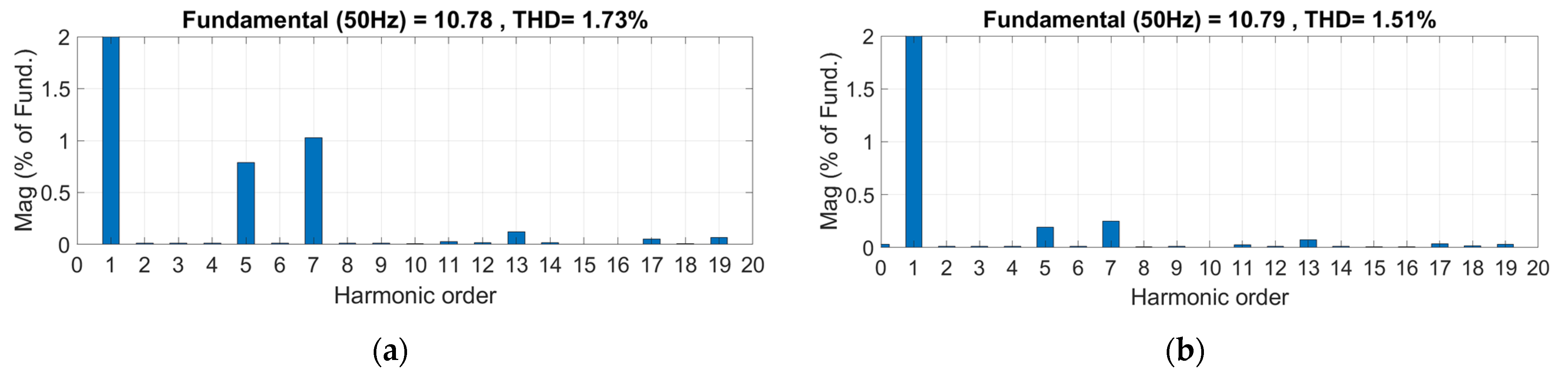
In this system, the extraction techniques are also tested by introducing delays that normally occur in the measurement path. A delay of 1 µs, which is equal to the simulation step size, is added to all measurement units including the voltage source measurement, the load current measurement, the injected harmonics measurement, and the source current measurement. Figure 11 and Figure 12 represent the FFT of the source current, including these delays for the SAPF using the different extraction techniques. It can be deduced from the results that delays can introduce errors and hence increase the source current THD. However, the MPM again achieves a lower source current THD of 1.51% compared to that of the PQ of 1.92% and SRF of 1.73%. These results are summarized in Table 3.
5.2.5. Asymmetrical Load Conditions
In this section, the MPM is evaluated under asymmetrical load conditions, where the asymmetrical load is added parallel to the existing non-linear load. For this purpose, an asymmetrical load (Ra = 25 Ω, Rb = 45 Ω, Rc = 55 Ω) is added parallel to the non-linear load at t = 0.5 s. The load current, harmonic current, and source current waveforms in addition to the DC-link voltage of the proposed method are shown in Figure 13. The results reveal the capability of the MPM to compensate the harmonics under asymmetrical load conditions, with a lower source current THD for each phase. This is summarized in Table 4 and compared to the PQ and SRF.
6. Conclusions
This paper proposed the MPM for reference signal extraction in active power filters that compensate source current harmonics by injecting the extracted signal at the PCC between the source and the load. The THD of the source current resulting from the extraction process was first studied for a reduced system, where the source current was obtained by directly subtracting the harmonics generated from the load current. The results showed that the conventional methods have their THDs dependent on the sample time step change, with best results of 0.21% for the PQ theory and 0.31% for the SRF. However, the MPM reduced the source current THD from 25.61% to almost zero independent of the sample time step, indicating that the MPM was more accurate than either the PQ or SRF. Also, in this reduced system the response time for the THD to reach steady state was studied and showed that the MPM had a faster response, as it reached its steady state THD after 0.04 s, whereas the PQ and SRF reached their steady-state THDs at 0.095 s and 0.055 s, respectively. The MPM was then evaluated for a complete system, taking into consideration a PWM control with 12.5 kHz switching frequency, a coupling inductor, and a capacitor in the DC-link. The obtained results showed that the MPM achieved a better performance by reducing the source current THD to a lower percentage than the other two methods for static, dynamic, and asymmetrical load conditions, even when measurement delays were introduced. As for the response time under the complete system, the MPM achieved a faster response than that of the PQ and a comparable response to that of the SRF.
Author Contributions
Conceptualization, A.E.G. and K.C.; methodology, A.E.G. and K.C.; software, A.E.G. and K.C.; validation, A.E.G., N.M., K.C. and M.T.; formal analysis, A.E.G.; resources, M.T. and N.M.; data curation, A.E.G. and K.C.; writing—original draft preparation, A.E.G. and K.C.; writing—review and editing, M.T. and N.M.; visualization, A.E.G.; supervision, K.C., M.T. and N.M. All authors have read and agreed to the published version of the manuscript.
Funding
This research received no external funding.
Institutional Review Board Statement
Not applicable.
Informed Consent Statement
Not applicable.
Data Availability Statement
Not applicable.
Conflicts of Interest
The authors declare no conflict of interest.
References
- Femine, A.D.; Gallo, D.; Giordano, D.; Landi, C.; Luiso, M.; Signorino, D. Power Quality Assessment in Railway Traction Supply Systems. IEEE Trans. Instrum. Meas. 2020, 69, 2355–2366. [Google Scholar] [CrossRef]
- De Santis, M.; Silvestri, L.; Vallotto, L.; Bella, G. Environmental and Power Quality Assessment of Railway Traction Power Substations. In Proceedings of the 2022 6th International Conference on Green Energy and Applications (ICGEA), Singapore, 4 March 2022; pp. 147–153. [Google Scholar]
- Dugan, R.C.; McGranaghan, M.F.; Santoso, S.; Beaty, H.W. Electrical Power Systems Quality, 3rd ed.; McGraw Hill: New York, NY, USA, 2012; ISBN 9780071761550. [Google Scholar]
- Jain, S. Control Strategies of Shunt Active Power Filter. In Modeling and Control of Power Electronics Converter System for Power Quality Improvements; Elsevier: Amsterdam, The Netherlands, 2018; pp. 31–84. ISBN 9780128145685. [Google Scholar]
- Lam, C.-S.; Choi, W.-H.; Wong, M.-C.; Han, Y.-D. Adaptive DC-Link Voltage-Controlled Hybrid Active Power Filters for Reactive Power Compensation. IEEE Trans. Power Electron. 2012, 27, 1758–1772. [Google Scholar] [CrossRef]
- Rashid, M.H. (Ed.) Power Electronics Handbook: Devices, Circuits, and Applications Handbook, 3rd ed.; Elsevier: Burlington, MA, USA, 2011; pp. 1193–1228. ISBN 9780123820365. [Google Scholar]
- Qazi, S.H.; Mustafa, M.W.B.; Soomro, S.; Larik, R.M. Comparison of Reference Signal Extraction Methods for Active Power Filter to Mitigate Load Harmonics from Wind Turbine Generator. In Proceedings of the 2015 IEEE Conference on Energy Conversion (CENCON), Johor Bahru, Malaysia, 19–20 October 2015; pp. 463–468. [Google Scholar]
- Akagi, H. Modern Active Filters and Traditional Passive Filters. Bull. Pol. Acad. Sci. Tech. Sci. 2006, 54, 255–269. [Google Scholar]
- Chen, D.; Xiao, L.; Yan, W.; Li, Y.; Guo, Y. A Harmonics Detection Method Based on Triangle Orthogonal Principle for Shunt Active Power Filter. Energy Rep. 2021, 7, 98–104. [Google Scholar] [CrossRef]
- Kashif, M.; Hossain, M.J.; Fernandez, E.; Taghizadeh, S.; Sharma, V.; Ali, S.M.N.; Irshad, U.B. A Fast Time-Domain Current Harmonic Extraction Algorithm for Power Quality Improvement Using Three-Phase Active Power Filter. IEEE Access 2020, 8, 103539–103549. [Google Scholar] [CrossRef]
- Das, S.R.; Ray, P.K.; Sahoo, A.K.; Ramasubbareddy, S.; Babu, T.S.; Kumar, N.M.; Elavarasan, R.M.; Mihet-Popa, L. A Comprehensive Survey on Different Control Strategies and Applications of Active Power Filters for Power Quality Improvement. Energies 2021, 14, 4589. [Google Scholar] [CrossRef]
- Hoon, Y.; Mohd Radzi, M.; Hassan, M.; Mailah, N. A Dual-Function Instantaneous Power Theory for Operation of Three-Level Neutral-Point-Clamped Inverter-Based Shunt Active Power Filter. Energies 2018, 11, 1592. [Google Scholar] [CrossRef] [Green Version]
- Büyük, M.; İnci, M.; Tan, A.; Tümay, M. Improved Instantaneous Power Theory Based Current Harmonic Extraction for Unbalanced Electrical Grid Conditions. Electr. Power Syst. Res. 2019, 177, 106014. [Google Scholar] [CrossRef]
- Patel, A.; Mathur, H.D.; Bhanot, S. A New SRF-Based Power Angle Control Method for UPQC-DG to Integrate Solar PV into Grid. Int. Trans. Electr. Energy Syst. 2019, 29, e2667. [Google Scholar] [CrossRef] [Green Version]
- Musa, S.; Radzi, M.; Hizam, H.; Wahab, N.; Hoon, Y.; Zainuri, M. Modified Synchronous Reference Frame Based Shunt Active Power Filter with Fuzzy Logic Control Pulse Width Modulation Inverter. Energies 2017, 10, 758. [Google Scholar] [CrossRef]
- Hoon, Y.; Mohd Radzi, M.A.; Mohd Zainuri, M.A.A.; Zawawi, M.A.M. Shunt Active Power Filter: A Review on Phase Synchronization Control Techniques. Electronics 2019, 8, 791. [Google Scholar] [CrossRef] [Green Version]
- Akagi, H.; Nabae, A.; Atoh, S. Control Strategy of Active Power Filters Using Multiple Voltage-Source PWM Converters. IEEE Trans. Ind. Appl. 1986, IA-22, 460–465. [Google Scholar] [CrossRef]
- Imam, A.A.; Sreerama Kumar, R.; Al-Turki, Y.A. Modeling and Simulation of a PI Controlled Shunt Active Power Filter for Power Quality Enhancement Based on P-Q Theory. Electronics 2020, 9, 637. [Google Scholar] [CrossRef]
- Buła, D.; Grabowski, D.; Maciążek, M. A Review on Optimization of Active Power Filter Placement and Sizing Methods. Energies 2022, 15, 1175. [Google Scholar] [CrossRef]
- Chahine, K. Towards Automatic Setup of Nonintrusive Appliance Load Monitoring—Feature Extraction and Clustering. Int. J. Electr. Comput. Eng. 2019, 9, 1002. [Google Scholar] [CrossRef]
- Chahine, K.; Baltazart, V.; Wang, Y. Interpolation-Based Matrix Pencil Method for Parameter Estimation of Dispersive Media in Civil Engineering. Signal Process. 2010, 90, 2567–2580. [Google Scholar] [CrossRef]
- Chahine, K.; Baltazart, V.; Wang, Y. Parameter Estimation of Dispersive Media Using the Matrix Pencil Method with Interpolated Mode Vectors. IET Signal Process. 2011, 5, 397. [Google Scholar] [CrossRef]
- Chahine, K.; Baltazart, V.; Wang, Y. Parameter Estimation of Damped Power-Law Phase Signals via a Recursive and Alternately Projected Matrix Pencil Method. IEEE Trans. Antennas Propag. 2011, 59, 1207–1216. [Google Scholar] [CrossRef]
- Fernandez del Rio, J.E.; Catedra-Perez, M.F. The Matrix Pencil Method for Two-Dimensional Direction of Arrival Estimation Employing an L-Shaped Array. IEEE Trans. Antennas Propag. 1997, 45, 1693–1694. [Google Scholar] [CrossRef]
- McClure, M.; Qiu, R.C.; Carin, L. On the Superresolution Identification of Observables from Swept-Frequency Scattering Data. IEEE Trans. Antennas Propag. 1997, 45, 631–641. [Google Scholar] [CrossRef]
- Qiu, R.C.; Lu, I.T. Multipath Resolving with Frequency Dependence for Wide-Band Wireless Channel Modeling. IEEE Trans. Veh. Technol. 1999, 48, 273–285. [Google Scholar] [CrossRef]
- IEEE Std 3002.8-2018; IEEE Recommended Practice for Conducting Harmonic Studies and Analysis of Industrial and Commercial Power Systems. IEEE: Piscataway, NJ, USA, 2018; ISBN 9781504451772.
Figure 1.
Three phase shunt active power filter Block Diagram.

Figure 2.
THD vs. Sample time.

Figure 3.
THD measurement vs. time in transient state at sample time 5 × 10⁻⁵ s (a) overall figure and (b) enlarged figure.
Figure 3.
THD measurement vs. time in transient state at sample time 5 × 10⁻⁵ s (a) overall figure and (b) enlarged figure.

Figure 4.
Waveforms of IL, Ih, and Is (a) using PQ extraction (b) using SRF extraction.

Figure 5.
Waveforms of IL, Ih, and Is using the proposed MPM extraction.

Figure 6.
FFT analyzer for source current (a) without APF (b) with APF using PQ extraction.

Figure 7.
FFT analyzer for source current (a) with APF using SRF extraction (b) with APF using MPM extraction.
Figure 7.
FFT analyzer for source current (a) with APF using SRF extraction (b) with APF using MPM extraction.

Figure 8.
DC-link capacitor’s voltage value PQ, SRF, and MPM.

Figure 9.
Waveforms and DC-link voltage during load change using MPM technique.

Figure 10.
FFT analyzer for source current with APF using MPM extraction at load change.

Figure 11.
FFT analyzer considering delays for source current (a) without APF (b) with APF using PQ extraction.
Figure 11.
FFT analyzer considering delays for source current (a) without APF (b) with APF using PQ extraction.

Figure 12.
FFT analyzer considering delays for source current (a) with APF using SRF extraction (b) with APF using MPM extraction.
Figure 12.
FFT analyzer considering delays for source current (a) with APF using SRF extraction (b) with APF using MPM extraction.

Figure 13.
Waveforms and DC-link voltage under asymmetrical load conditions using MPM technique.


Table 1.
Circuit Parameters.
| Parameter | Value |
|---|---|
| Supply frequency | 50 Hz |
| Peak value of phase supply voltage | 220 V |
| Source resistance (Rs) | 0.15 Ω |
| Source inductance (Ls) | 0.03 mH |
| Line resistance (Rr) | 1 Ω |
| Line inductance (Lr) | 1 mH |
| Load resistance (RL) | 40 Ω |
| Load inductance (LL) | 2 mH |
| Coupling inductance (Lf) | 3 mH |
| DC-Link capacitance (Cdc) | 3000 µF |
| DC-Link reference voltage | 700 V |
Table 2.
Source Current % THD comparison.
| Extraction Method | % THD of Source Current |
|---|---|
| No Filter | 25.61% |
| PQ | 1.21% |
| SRF | 1.43% |
| Proposed MPM | 0.85% |
Table 3.
Source Current % THD comparison including delays.
| Extraction Method | % THD of Source Current |
|---|---|
| No Filter | 25.60% |
| PQ | 1.92% |
| SRF | 1.73% |
| Proposed MPM | 1.51% |
Table 4.
Source Current % THD comparison under asymmetrical load conditions.
| Extraction Method | % THD of Source Current | ||
|---|---|---|---|
| Phase a | Phase b | Phase c | |
| PQ | 1.09% | 2.01% | 1.84% |
| SRF | 3.32% | 3.77% | 3.79% |
| Proposed MPM | 0.59% | 1.08% | 0.74% |
Publisher’s Note: MDPI stays neutral with regard to jurisdictional claims in published maps and institutional affiliations. |
© 2022 by the authors. Licensee MDPI, Basel, Switzerland. This article is an open access article distributed under the terms and conditions of the Creative Commons Attribution (CC BY) license (https://creativecommons.org/licenses/by/4.0/).
Share and Cite
MDPI and ACS Style
El Ghaly, A.; Tarnini, M.; Moubayed, N.; Chahine, K. A Filter-Less Time-Domain Method for Reference Signal Extraction in Shunt Active Power Filters. Energies 2022, 15, 5568. https://doi.org/10.3390/en15155568
AMA Style
El Ghaly A, Tarnini M, Moubayed N, Chahine K. A Filter-Less Time-Domain Method for Reference Signal Extraction in Shunt Active Power Filters. Energies. 2022; 15(15):5568. https://doi.org/10.3390/en15155568
Chicago/Turabian StyleEl Ghaly, Abdallah, Mohamad Tarnini, Nazih Moubayed, and Khaled Chahine. 2022. "A Filter-Less Time-Domain Method for Reference Signal Extraction in Shunt Active Power Filters" Energies 15, no. 15: 5568. https://doi.org/10.3390/en15155568
Note that from the first issue of 2016, this journal uses article numbers instead of page numbers. See further details here.