
A New Uncertainty-Based Control Scheme of the Small Modular Dual Fluid Reactor and Its Optimization


1
Chair of Nuclear Technology, Department of Mechanical Engineering, Technical University of Munich (TUM), 85748 Garching, Germany
2
School of Resource & Environment and Safety Engineering, University of South China, Hengyang 421001, China
*
Author to whom correspondence should be addressed.
Energies 2021, 14(20), 6708; https://doi.org/10.3390/en14206708
Submission received: 2 August 2021
/
Revised: 1 October 2021
/
Accepted: 10 October 2021
/
Published: 15 October 2021
(This article belongs to the Special Issue Advances in Fluid Power Systems)
Abstract
:The small modular dual fluid reactor is a novel variant of the Generation IV molten salt reactor and liquid metal fast reactor. In the primary circuit, molten salt or liquid eutectic metal (U-Pu-Cr) is employed as fuel, and liquid lead works as the coolant in the secondary circuit. To design the control system of such an advanced reactor, the uncertainties of the employed computer model and the physicochemical properties of the materials must be considered. In this paper, a one-dimensional model of a core is established based on the equivalent parameters achieved via the coupled three-dimensional model, taking into account delayed neutron precursor drifting, and a power control system is developed. The performance of the designed controllers is assessed, taking into account the model and property uncertainties. The achieved results show that the designed control system is able to maintain the stability of the system and regulate the power as expected. Among the considered uncertain parameters, the reactivity coefficients of fuel temperature have the largest influence on the performance of the control system. The most optimized configuration of the control system is delivered based on the characteristics of uncertainty propagation by using the particle swarm optimization method.
1. Introduction
The dual fluid reactor, which adopts molten salt or liquid eutectic metal (U-Pu-Cr) as fuel and liquid lead as a coolant, has a considerable number of advantages over conventional reactors. It is a novel variant of the Generation IV molten salt reactor and liquid metal fast reactor. A relevant study can be traced back to 1966, when a two-fluid molten salt breeder reactor (MSBR) was designed at Oak Ridge National Laboratory [1]. The proposed MSBR was investigated for its load-following capability under various ramp rates of the power demand without a controller [2], and its enlarged version of 2 GW thermal output was proposed by Taube et al. in 1974 [3]. Later, a new design of the two-fluid molten salt reactor, named the dual fluid reactor (DFR), was proposed by researchers at the Institue for Solid-State Nuclear Physics (IFK) [4]. By using liquid lead, the dual fluid reactor has a high capability to transfer heat produced in the core and can be operated at a considerably high power density without any safety issues. The characteristics of the steady-state physics of the dual fluid reactor concept were investigated [5,6], and a comparative study of the two fuel options was conducted [7]. The distribution zone of the dual fluid reactor concept has been designed and analyzed from the perspective of thermal hydraulics [8,9]. According to previous studies, the dual fluid reactor concept has a unique feature. Based on this fact, special attention has to be paid to the design and optimization of its control system to ensure that the reactor is able to follow the load as desired and has little overshoot/fluctuation as possible. However, to date, research on the control system of the dual fluid reactor concept has not been conducted, and the strategy for optimization of the controller is unknown. Moreover, the uncertainties introduced during the modeling process must be considered to ensure that the optimized control system is always reliable in spite of the deviations between the numerical model and reality.
In this work, a one-dimensional model of the core of the small modular dual fluid reactor (SMDFR) is built based on the equivalent parameters achieved by the coupled three-dimentional model, taking into account delayed neutron precursor (DNP) drifting, and a power control system is developed. Then, the most representative uncertain parameters of this model are chosen based on the experience of a previous study [10], and their influences on the numerical model are quantified. Finally, the technique of particle swarm optimization (PSO) is implemented to optimize the controller of the core considering its uncertainties.
2. Description of SMDFR and Control System
2.1. Small Modular Dual Fluid Reactor
Unlike the original dual fluid reactor design, the nominal power of the small modular dual fluid reactor was reduced to: = 0.1 GW = 100 MW , which is much lower compared to the original designed thermal power of 3 GW. The schematic of the SMDFR is shown in Figure 1. There are three circuits in the schematic: the primary circuit of molten salt as fuel is depicted in deep red; the secondary circuit of liquid lead as the primary coolant is depicted in yellow; and the tertiary circuit of liquid lead as the secondary coolant is depicted in blue. The mass flow rate of the molten salt in the primary circuit is notably low and is intended solely for online fuel processing instead of heat removal. The heat produced by fission in the core is majorly taken by the liquid lead as the primary coolant in the secondary circuit and then transferred to the secondary coolant in the tertiary circuit for utilization, such as hydrogen production, electricity generation, and water desalination.
In this work, the core of the SMDFR is chosen as the research object, which is made of three parts: the distribution zone, core zone, and collection zone. Starting from the bottom part of the core, the fuel (molten salt) goes into the distribution zone, flows through the core zone, and then leaves the collection zone. The coolant (liquid lead) flows in the same direction and takes heat generated by the fission reaction taking place in the molten salt. Since this work focuses on the one-dimensional model of the core, a detailed description of the geometry is beyond the scope of this paper, and the reader is referred to the literature [9].
The major design parameters are listed in Table 1. In this work, the molten salt, which is a mixture of uranium tetrachloride and plutonium tetrachloride, is selected as fuel, and silicon carbide is employed as the pipe wall.
2.2. Uncertainty-Based Particle Swarm Optimization of the Control System
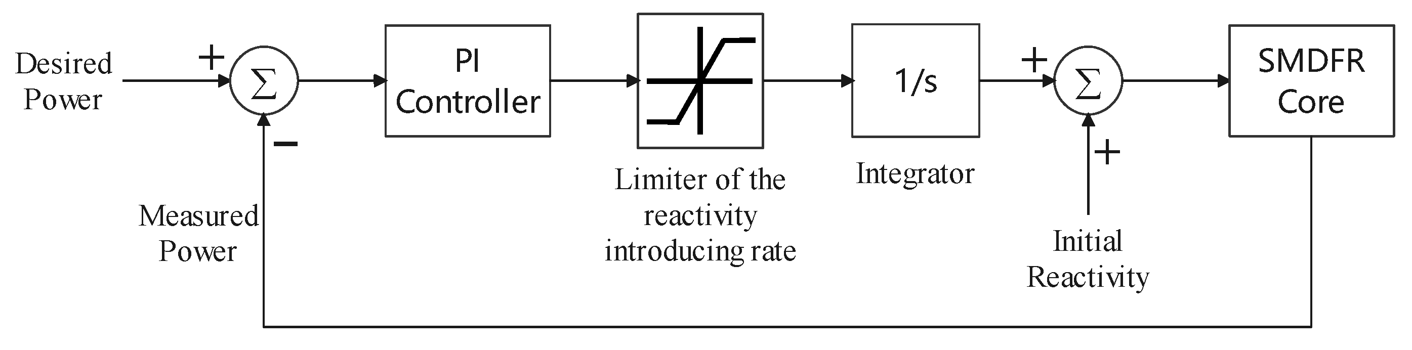
A control system is designed for the control of power of the SMDFR. Its working principle is shown in Figure 2. The desired power is determined based on the load demand and then compared with the measured power. Their difference is sent to the PI controller to adjust the value of reactivity to be introduced. It can be observed that a limiter of ±15 pcm/s is applied to limit the introduction rate of reactivity, considering the criticality safety of the core and engineering feasibility [11]. The reactivity is assumed to be introduced by the control rod and applied uniformly to the whole core. As initial values, Kp is set to 200 and Ki is set to 50. Firstly, the feasibility of the designed control system is investigated, and then optimization of the examined control system is conducted.
To achieve the best performance, the particle swarm optimization technique is employed to settle the PI parameters for the control system. The uncertainties of the model and property have to be quantified to ensure that the optimization is always valid. The structure of the uncertainty-based PSO optimization of the PI controller is shown in Figure 3.
3. Methodology
In this work, a one-dimensional model of the SMDFR core is established based on the equivalent parameters achieved by the coupled three-dimensional model, taking into account the delayed neutron precursor drifting by modifying the point kinetic model. The reactivity feedback, resulting from the temperature and density change in the two fluids, is considered by a linearized correlation of the introduced reactivity and the changed temperatures. After finishing the core model, a PI controller is added to control the power via the introduction of positive or negative reactivity based on the difference between the set value and the measured value of core power. Finally, the uncertainty-based control system is designed and optimized using the PSO technique considering the uncertainty quantification.
3.1. Reactor Core Modeling
In order to obtain basic data for the establishment of the one-dimensional model of the SMDFR core, the parameters needed for the neutronic and thermodynamic equations are acquired from the coupled three-dimensional model. In addition, the point kinetic model has to be modified to accurately describe the process of delayed neutron precursor drifting. The thermodynamic model is built based on the assumption that the fuel, the piping wall, and the coolant in the core are divided into 12 parts and each part has lumped properties. The point kinetic model and the thermodynamic model are then linked by the reactivity feedback.
3.1.1. Data Used for Analysis
For the simulation, two types of data are required, the neutronics data (Table 2) and the thermodynamics data (Table 3). The neutronics data are obtained by using Serpent 2.1.31 with the ENDF/B-VII nuclear data library, applying the calculated temperature and density distributions of the fuel and coolant. The thermodynamics data are calculated using the fully resolved CFD model via COMSOL Multiphysics version 5.6 [12] together with its CFD module [13] and heat transfer module [14].
3.1.2. Modified Point Kinetic Model
In order to accurately capture the neutronic behavior of the SMDFR, the point kinetic model [15] with 6 delayed neutron groups (i = 1, ..., 6) is adopted and modified. Although the fuel outside of the core is kept subcritical, the decay process of delayed neutron precursors has to be considered to describe its influence on neutron distribution in the core. Traditionally, the effect of the delayed neutrons due to the flowing fuel is described by two additional terms [16]: the precursor loss when the fuel leaves the core, and the precursor gain when the fuel re-enters the core, which are the 3rd and the 4th terms on the right side of the delayed neutron precursors equations, respectively, as shown in Equation (1). However, the time delay term introduces some complexities to the modeling process, and some special treatments have to be applied to solve this kind of equation. To eliminate this time delay term, the concentrations of the six groups of delayed neutron precursors outside of the core, , are defined, and then the balance of delayed neutron precursors can be described as shown in Figure 4. The concentrations of the six group delayed neutron precursors inside the core can be given by Equation (2). Since six depend variables are introduced, an additional six equations (Equation (3)) describing the evolution of the DNP concentrations outside of the core, together with the equation of the neutron density (Equation (4)), have to be added to close the set of equations for the point kinetic model.
3.1.3. Thermodynamic Model
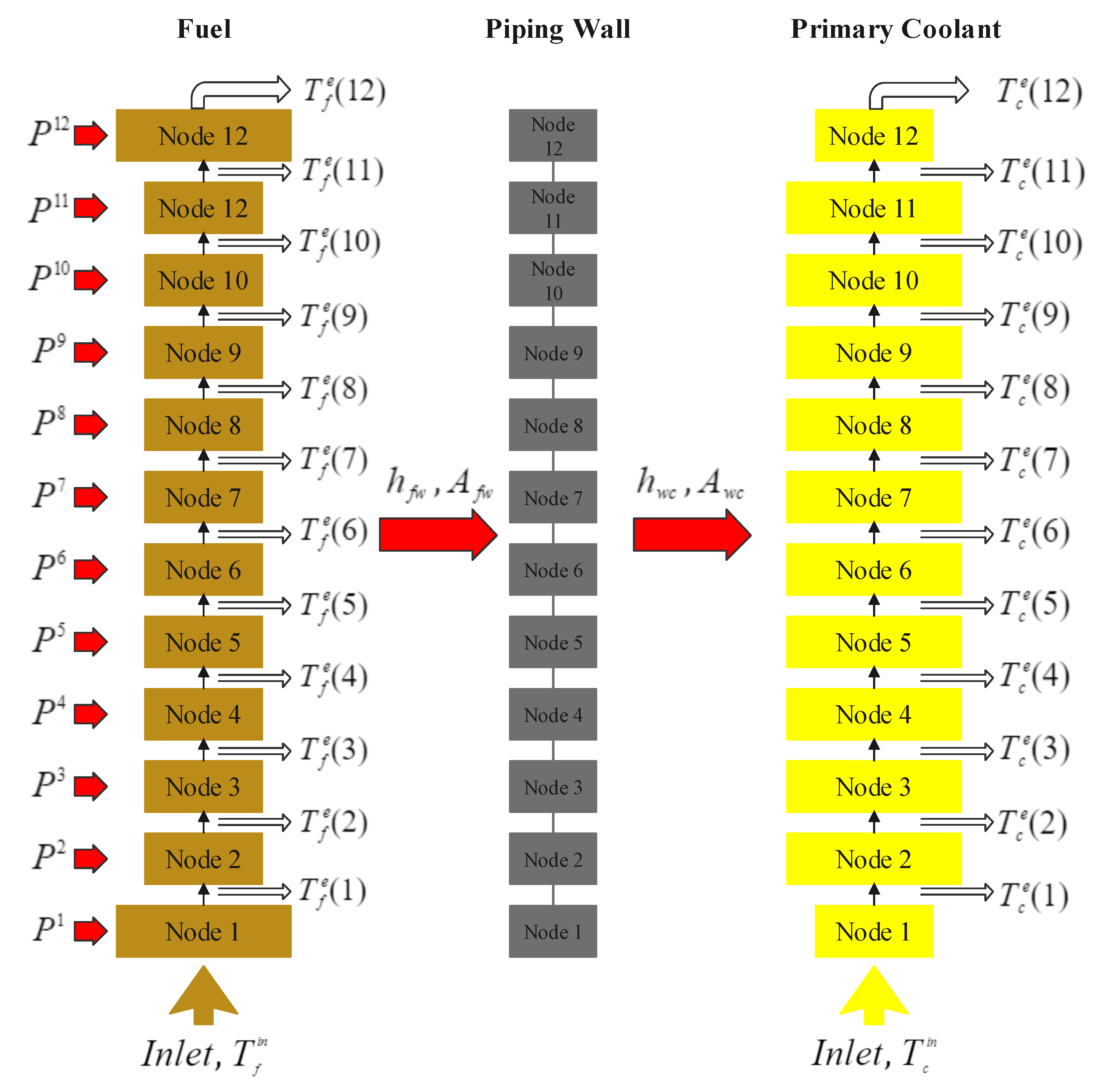
Considering the geometry structure of the core, 12 nodes are defined: Node 1 for the distribution zone, Node 2–11 for the core zone, and Node 12 for the collection zone, as shown in Figure 5. Each node has a height of 0.2 m. The energy balance of Node 1 is described by Equations (8)–(10). For the remaining nodes (Node 2–12, i = 2, ..., 12), the heat transfer process is governed by Equations (11)–(13). As shown in Figure 5, the heat generated by the nuclear fission is transferred from the fuel to the piping wall and then to the primary coolant. Finally, the fission energy is taken by the primary coolant and transferred to the secondary coolant for utilization. The power is assumed to be proportional to the neutron density, as shown in Equation (14).
3.1.4. Reactivity Feedback
The change in temperatures of the fuel or coolant introduces additional reactivity, which is called reactivity feedback, and it has an important impact on the operation of the reactor. The reactivity consists of the initial reactivity, the reactivity introduced by the variation in temperatures of the fuel and coolant, and the externally inserted reactivity from control rods or other sources, as shown by Equation (15):
where is the temperature feedback coefficient of fuel; is the temperature feedback coefficient of the coolant; and are the initial mean temperatures of the fuel and coolant, respectively; and and denote the real time mean temperatures.
3.2. PI Controller
In this work, the PI controller is adopted for the control system. As a variation of proportional integral derivative (PID) control, only the proportional and integral terms are used in proportional integral (PI) control. The difference between the set value and the real (measured) value, , is given to the PI controller as the feedback error, and then the value of the controller output is calculated in the time domain from the feedback error by Equation (17) and then fed into the system as the manipulated variable input. It is clear that the two parameters and have a significant influence on the system response and, thus, should be optimized for the best control performance.
3.3. Uncertainty Quantification
In order to quantify the system uncertainties, the input uncertainties of the system must be identified, and their ranges and probability densities function must be determined. Several methods are available for the quantification of uncertainty, but the nondestructive technique, tolerance limits [17], is selected in this work considering its reduced consumption of computational resources. The Monte-Carlo method, which is much more computationally expensive, is used to verify the performance of the delivered control system.
3.3.1. Input Uncertainties of the Numerical Model
Regardless of the accuracy that the numerical model can achieve, since approximations and assumptions are essential in the modeling and calculation process, a degree of uncertainty is always expected and has to be well quantified to deliver reliable results with adequate assurance. However, since not all of the uncertain parameters can be considered due to the limited computational resources and the limited knowledge, only the most representative uncertain parameters are taken into account based on the experience of a previous study [10]. Their influences on the numerical model have to be quantified and considered during the design and optimization of the control system.
The selected uncertain parameters, which are considered as the input of the uncertainty quantification procedure, were assumed to be uniformly distributed in their ranges and are given in Table 4. The ranges are determined in the following manner:
- Thermal power, mass flow rates, and inlet temperatures are specified with reference to the reported experimental uncertainty in the literature [18].
- The heat capacity of liquid lead (coolant) is specified according to the uncertainty bounds found in [19].
- The heat capacity of molten salt (fuel) is specified referring to the value of liquid lead. Since no data are available for the molten salt, and there is a heat transfer process between the two fluids, a consistent uncertainty range is applied to both of them in order to achieve a conservative assumption for the heat transfer process. In the future, its value will be adapted when experimental data of the molten salt are generated/available.
- Temperature feedback coefficients and heat transfer coefficients are taken with a ±10% uncertainty range from the default value. Since no data are available, this assumption is considered to be sufficiently conservative. When more data are obtained, their ranges will be updated accordingly.
3.3.2. Tolerance Limits
The idea of applying tolerance limits for uncertainty quantification was proposed by Glaeser [17]. By employing this technique, the required sample size, which is the required runs of the computer model, is reduced, while the resulting statistical interval binds with confidence (usually 95%). According to the definition made by Krishnamoorthy and Mathew [20], two types of tolerance limits can be achieved: one-sided tolerance limits and two-sided tolerance limits.
The upper/lower tolerance limit can be explained as follows: the upper/lower confidence limit can be granted for at least the percentile of the population. A percentage of the population would be bounded by the upper/lower tolerance limit with a confidence of .
The two-sided tolerance limits can be explained as follows: The two-sided confidence limits can be granted for at least the percentile of the population. A percentage of the population would be bounded by the two-sided tolerance limits with a confidence of .
The confidence level can be calculated by [21]
When a one-sided upper/lower tolerance limit is considered, has to be set to 0. When two-sided tolerance limits are expected, normally, r is set to be equal to s to ensure a consistent grade of upper and lower limits. Given r, s, p (population proportion of interest) and , the required sample size (N) is given by Equation (18).
In this work, 59 runs were performed to obtain the one-sided upper tolerance limit based on the 1D computer model. Making the confidence level equal to 0.95, the population proportion of interest p would be 0.95 according to Equation (18).
3.3.3. Sensitivity Quantification
The effect of the sensitivity of input uncertainty on the system output can be investigated by the following four types of methods: graphical methods, screening analysis, regression-based analysis, and variance-based analysis. The sensitivity is quantitatively analyzed by the latter two methods in this paper, as the former two methods are qualitative.
Regression-based techniques are often used to quantitatively analyze sensitivity when the system has a linear response between the input and output. The computational cost is lower than that of the variance-based technique. In this work, the standardized regression coefficient (SRC), which is given by Person’s ordinary correlation coefficients (Equation (19)) based on standardized variables (Equation (20)), is selected as the index to quantify the importance of input variables. The squared value of SRC is considered to be the fraction of the output variance linearly explained by the input [22]. The coefficient of multiple determination [23] (Equation (21)) is used to examine the linearity of this relationship. Only when it is larger than 0.6 (cut-off value) can a high enough fraction of the output variability be explained by the input variability under a linear relation. The closer its value to 1.0, the more significant the linear relationship.
The variance-based technique (Sobol indices) was proposed by Ilya M. Sobol [24,25]. The output variance is decomposed, and the contribution of each input variable to output variance is identified by a certain percentage. This technique can quantify the global sensitivity regardless of whether or not the system is linear, while the interaction between input variables properly occurs. The major drawback of this method is the high computational cost: , where k denotes the amount of input variables and N denotes the sample size, with a value typically larger than 1000. By defining two commonly used Monte-Carlo estimators, S1 and ST, the first-order sensitivity index and the total effect index [25,26], the sensitivity can be quantified taking into account the linear and non-linear relationships. A detailed discussion of the Sobol method is beyond the scope of this paper; more details on its algorithm and estimators can be found in the literature [10].
3.4. PSO Optimization with Uncertainties
Particle swarm optimization is a technique used to optimize a problem [27]. By moving the candidate particles in the search space according to the defined formula, the particles are guided toward the best positions based on a given criterion. Finally, the best position will be found as the optimal solution. Since this paper focuses on the uncertainty-based design and optimization of the control system, a more detailed discussion of the algorithm of particle swarm optimization and its development is beyond the scope of this work. Further details can be found in the literature [27,28,29]. In this work, the Matlab toolbox, Constrained Particle Swarm Optimization version 1.31.4 [30], is used for the PSO algorithm.
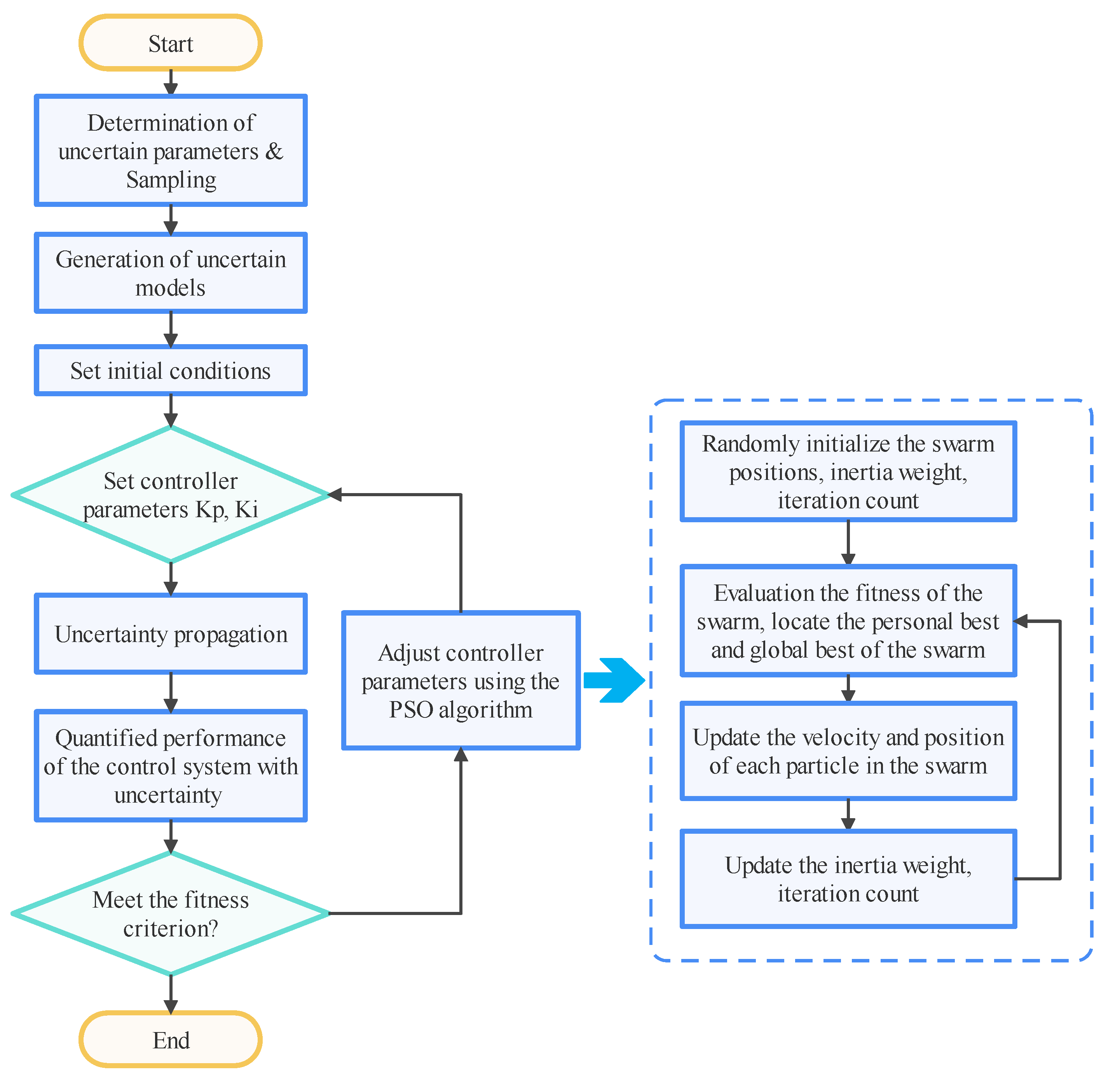
The process of the PSO algorithm with uncertainties of the control system is shown in Figure 6. Firstly, the input parameters are sampled based on the given distributions shown in Table 4, and then the initial conditions of the computer models are set. After setting the controller parameters, the system uncertainty is quantified, and then the performance of the given control system is assessed. By continuously adjusting controller parameters using the PSO algorithm, the optimized control system considering the existence of uncertainty will be achieved. Notably, not only can this working flow be applied to the design of the control system of the nuclear system, but it can also be used for the control system of any other energy systems subjected to uncertainties.
4. Results and Discussion
The Results and Discussion Section is divided into four parts: verification, feasibility of the control system, optimization, and performance assessment.
4.1. Verification
Since the SMDFR is a new concept, and no experimental data are available at this stage, the 1D Matlab model has to be verified against the high-fidelity 3D COMSOL model. A comparison is shown in Figure 7, where asterisks represent the temperature of fuel, the downward-pointing triangle represents the temperature of piping wall, and the cross represents the temperature of the coolant. The results from COMSOL model are depicted in red and those from the Matlab model in black. Taking the COMSOL model as a reference, it can be seen that the shapes of temperature distributions of fuel, the piping wall, and the coolant are generally well captured by the Matlab model. Besides Node 12, the temperature differences in all of the other nodes are within ±20C. Matlab model was demonstrated to have sufficient capacity to capture the system behaviors and correctly predict the temperature distributions, which means that this 1D Matlab model can be used for the design and investigation of the control system.
4.2. Feasibility of the Control System
In order to investigate the feasibility of the control system, three transients, with and without the control system, are calculated: ±100 pcm insertion of reactivity, ±20 C variation in the inlet temperature, and ±10% variation in the coolant mass flow rate.
The results of the system response for ±100 pcm insertion of reactivity are shown in Figure 8. The power evolution of the system without a control system is depicted in red and that with a control system in black. Without a control system, as shown in Figure 8a, 100 pcm reactivity is inserted into the core at t = 10 s, causing the power to increase by around 6%. Since more power is generated to heat the fuel and coolant, their temperatures are increased. Due to the negative reactivity feedback of the fuel and coolant, a negative reactivity is introduced, and, thus, the power returns to 102.5% of its nominal power and stays constant at this level. However, the power level changes due to this perturbation, which is not preferred during the normal operation when an unchanged power level is expected despite perturbation. With the control system, the power goes back to its nominal value after several oscillations, and the peak value of the power is 1% lower than that without a control system. For the transient with –100 pcm reactivity insertion (Figure 8b), the system with a control system is also capable of retaining the nominal power after perturbation. For both cases, the time needed for the system to go back to its original state is within 150 s.
The results of the system response for ±20 C variation in the inlet temperature are shown in Figure 9. Without a control system, as shown in Figure 9a, the coolant inlet temperature increases by 20 C at t = 10 s, causing the power to decrease by around 8% due to the negative reactivity feedback of the coolant. The decreased power results in a decrease in fuel temperature. Thus, the negative reactivity introduced by the coolant is countered by the positive reactivity introduced by the decrease in fuel temperature. Finally, the power stays constant at the level of 92.5% of its nominal power. With a control system, the power returns to its nominal value after several oscillations, and the peak value of the power is 1% lower than that without a control system. For the transient with the decrease of 20 C (Figure 9b), the system with a control system is also capable of retaining the nominal power after perturbation. For both cases, the time needed for the system to return to its original state is 150 s.
The results of the system response for ±10% variation in the coolant mass flow rate are shown in Figure 10. Without a control system, as shown in Figure 10a, the coolant mass flow rate increases by 10% at t = 10 s, causing the power to increase by around 4%. As soon as the coolant mass flow rate increases, the heat transfer between the fuel and coolant enhances, and their temperatures thus decrease, resulting in an introduction of positive reactivity due to the negative reactivity feedback. Once the power increases, the temperatures of fuel and coolant increase, and, then, the introduced positive reactivity is countered by the negative reactivity introduced due to the temperature increase in the fuel and coolant. Finally, the power stays constant at the level of 100.4% of its nominal power. With a control system, the power returns to its nominal value after several oscillations, and the peak value of the power is 1% lower than that without a control system. For the transient with the decrease in the coolant mass flow rate (Figure 10b), the system with a control system is also capable of retaining the nominal power after perturbation. For both cases, the time needed for the system to return to its original state is 150 s.
4.3. Optimization
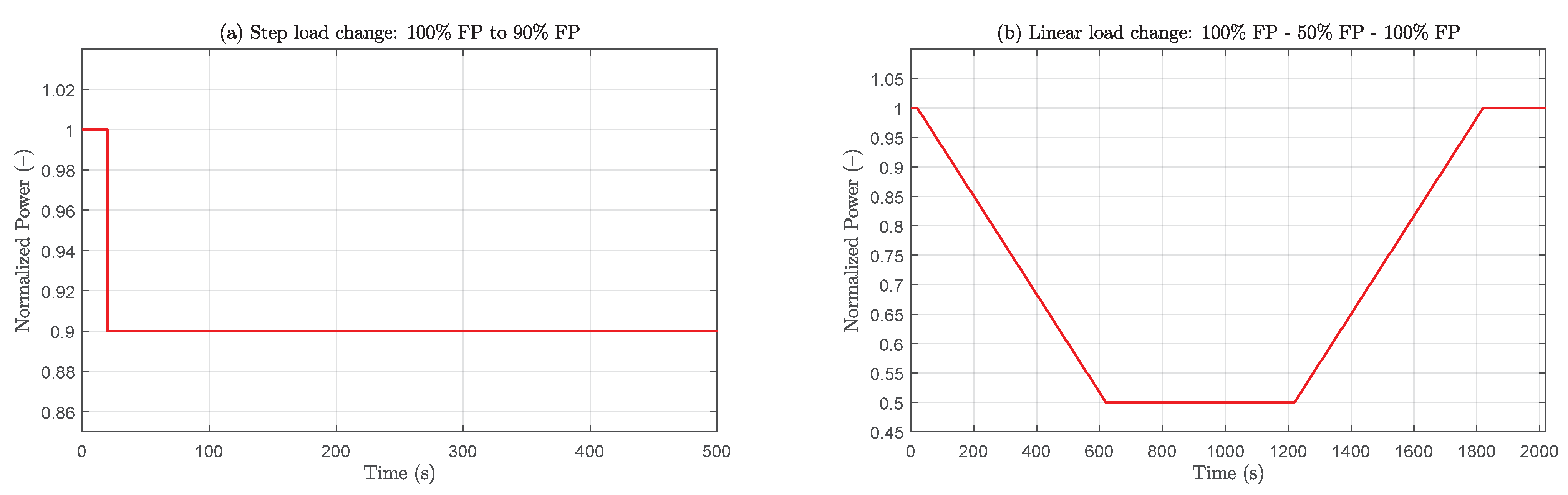
Although the control system is proved to be capable of handling various transients, its parameters have to be optimized to achieve the best performance. For the optimization of the control system, two scenarios are selected as benchmark cases: step load change: 100% FP to 90% FP; linear load change: 100% FP to 50% FP to 100% FP, as shown in Figure 11.
The integral time-weighted absolute error (ITAE), as defined by Equation (22), is selected as the criterion of performance of the control system for the case of step load change, since the errors that exist after a long time have to be weighted much more heavily than those at the start of the transient. For linear load change, the integral absolute error (IAE), as defined by Equation (23), is chosen as the criterion of performance, since the error should not be time weighted in this case any more. For both cases, the uncertain parameters in Table 4 are used to calculate the one-sided upper tolerance limit of the ITAE, which is chosen as the output of the fitness function of the PSO process. The achieved optimized solution has the following meaning: under the given uncertainty parameter ranges, at least 95% of the possible system states would have a better performance than that of the final optimized value achieved from the PSO process, with a probability of 95%. By applying the optimized parameters, the control system has a probability of 95% to deliver an optimized performance for more than 95% of the system states.
where is the error between the measured value of the controlled variable and its desired value.
4.3.1. Step Load Change
The major parameters for the PSO process are shown in Table 5. After 232 generations, the average cumulative change in the value of the fitness function over 50 generations is less than , and the final best point is: Kp = 7723.2, Ki = 872.29, with a fitness value of 70.78. The evolution of fitness value during the PSO process is shown in Figure 12, where the maximum and minimum values of the particles in each generation are depicted by the error bar. For the first 60 generations, large variations can be observed, as the particles were going through the entire domain to identify the best point (Figure 13). Then, they started to focus on a smaller region, where the best point can be found. After 130 generations, all particles were close to the final best point, and the optimization process finished after 232 generations.
4.3.2. Linear Load Change
The major parameters for the PSO process are kept the same as those for the step load change, as shown in Table 5. After 66 generations, the average cumulative change in the value of the fitness function over 50 generations is less than , and the final best point is: Kp = 10,000.0, Ki = 1000.0, with a fitness value of 0.014. The evolution of fitness value during the PSO process is shown in Figure 14, where the maximum and minimum values of the generation are depicted by the error bar. Unlike the step load change, the particles found the location of the best point after only 20 generations (Figure 15), and the optimization process was terminated after 66 generations. The amount of generation needed to identify the best point is much lower, since it is not so challenging for the control system to follow the load for the linear load change. Without the preset limits, Kp and Ki would obtain other values since they already reached their limits. However, the integral absolute error considering the limits lies below 0.015, which means that a well-optimized control system is obtained and no further optimization is necessary.
4.4. Performance Assessment
The performance of the optimized control system must be assessed considering its uncertainty and compared with its performance before optimization. Unlike the tolerance limits technique used in the optimization process, a Monte-Carlo method is adopted to assess the performance before and after optimization: 1000 uncertain runs are performed, and their confidence intervals (95% confidence) for quantiles 95% and 5% are chosen as the upper and lower boundaries, respectively.
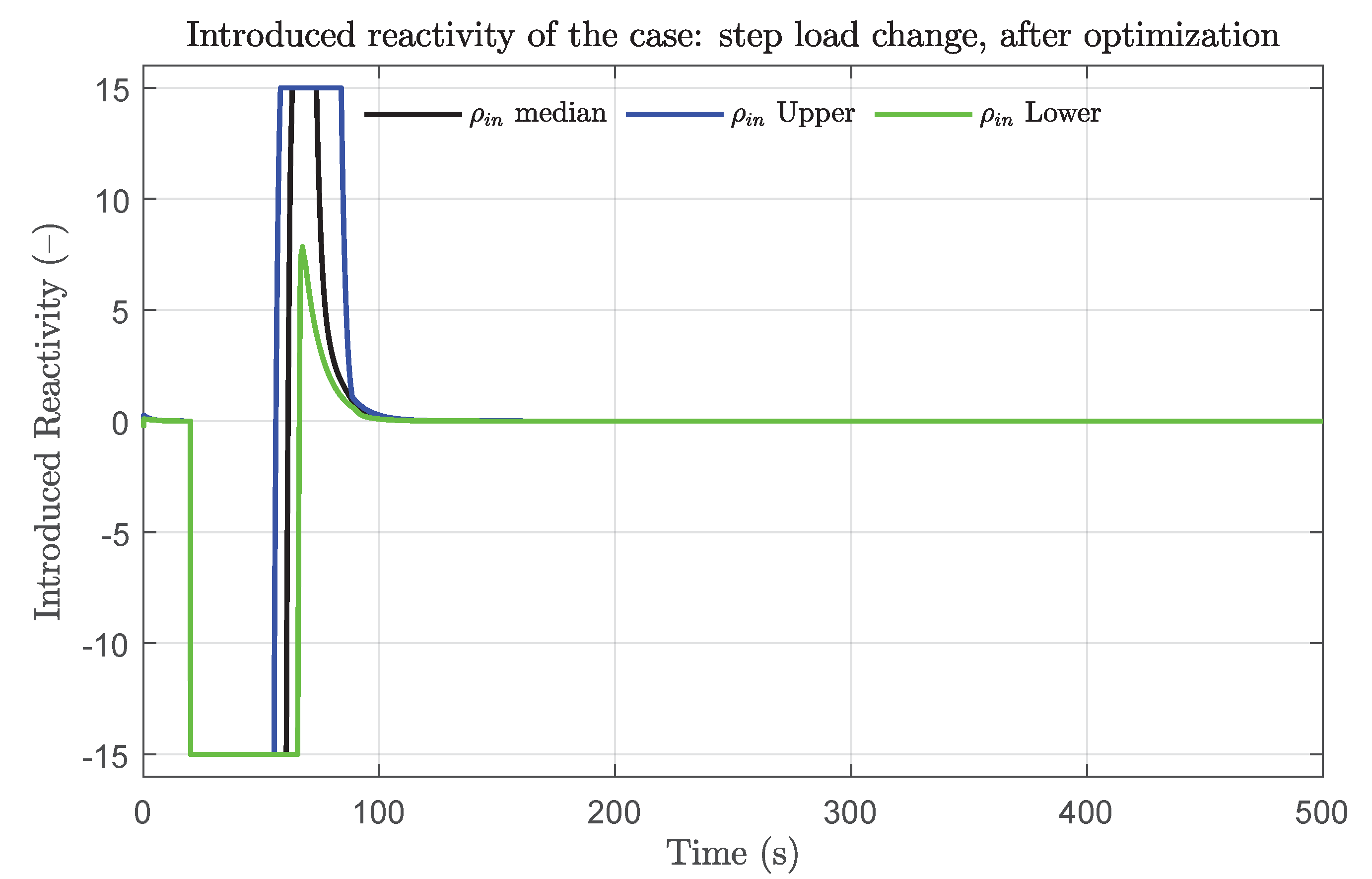
For step load change, the control system-introduced reactivity during the transient is shown in Figure 16, and the system responses before and after optimization are shown in Figure 17. The desired value is depicted in red; the median value of the real power (system response) is depicted in black; the blue and green lines depict the upper (95%) and lower (5%) uncertain boundaries of the system response, respectively.
The evolution of the introduced reactivity after optimization can be found in Figure 16. In the first stage of the transient (from t = 10 s to t = 60 s), the introduced reactivity reached its lower limit (–15 pcm/s), as the PI controller tried to eliminate the error introduced by the step signal as much as possible and thus made the output value equal to its lower limit to decrease the power. In the second stage (from t = 60 s to t = 90 s), since the reactor power was decreased by the introduced negative reactivity in the first stage, the fuel and coolant temperatures were lower than their original values. Due to the negative reactivity feedback coefficient of both fluids (Table 2), an additional positive reactivity was introduced and thus made the power higher than the set value. In order to counteract this effect, the PI controller switched its output from the lower limit to the upper limit (15 pcm/s) to reduce the reactor power. Finally, the power reached its set value at a new steady-state, and then the output signal of the PI controller returned to zero.
It is clear that the system response cannot be presented by a single fixed curve in time but by a region that is bounded by the upper and lower uncertain boundaries, which means that the system performance cannot be assessed by a simple curve but can be achieved based on the results of statistics with a certain confidence. However, after optimization, the performance of the control system is largely improved, as shown in Figure 17b, despite the existence of uncertainty, as it has a lower overshoot, less oscillation, and less time consumed to reach the new steady state.
The integral time-weighted absolute errors before and after optimization are shown in Figure 18. Before optimization, the upper boundary, the largest value that the system could deliver taking into account the existence of uncertainty with a confidence of 95%, is around 252.6 s, and its value is reduce to 70.5 s after optimization, which is consistent with the results presented in Section 4.3. Considering the uncertainties of the computer model and the physicochemical properties, the integral time-weighted absolute error of the optimized system has a probability of 95% to stay below 71 s with a confidence of 95%.
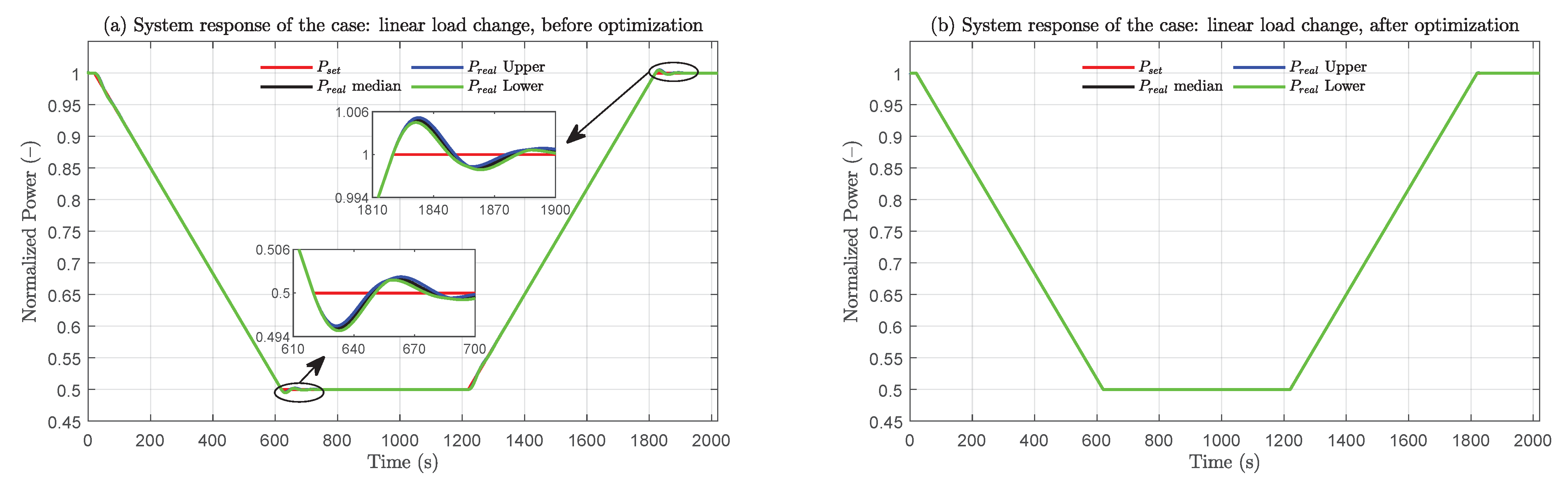
The system responses and IAE of the second case: linear load changes are shown in Figure 19 and Figure 20. It can be seen that the system response matches the desired power very well, and there is almost no discrepancy between the curves, which means that the control system can adjust the power according to the linear load change without any significant deviations or oscillations. However, before optimization, minor oscillations are observed right after the power ramps, which are eliminated after optimization.
The upper boundary of IAE is reduced from 0.7 s to 0.014 s through optimization. Considering the uncertainties, the integral absolute error of the optimized system has a probability of 95% to stay below 0.014 s with a confidence of 95%.
4.5. Sensitivity Analysis
As shown in Figure 21, parameter 2, the temperature feedback coefficient of fuel, has a major influence on the performance of the control system. The reason is that this feedback on reactivity plays an important role in adjusting neutron flux, and, thus, the power changes. Moreover, since its value is several times larger than that of other reactor concepts due to the large expansion rate of molten salt, its impact on power is significant, and determining its value should be prioritized to deliver a reliable model with less uncertainty. Moreover, parameter 8, the heat transfer coefficient between fuel and wall, has a non-negligible influence on output power. Careful calibration of the heat transfer coefficient has to be conducted in order to reduce the output uncertainty introduced by the heat transfer process. Since the coefficient of multiple determination is fairly close to 1.0, the system response can be assumed to be totally linear. This means that the results delivered by the regression-based technique have the same high quality as those from the variance-based technique. However, this does not imply that the system model is linear. This linear relationship can be only applied between the input variables and the selected system response: performance of the control system. From Figure 21b it can be observed that for parameter 2 and 8, the total effect indices, ST, are slightly higher than the first-order sensitivity indices, S1, which means these two parameters have certain co-effects on the system response together with other parameters, and these effects are captured by the total-effect indices.
Another option to reduce uncertainty is the application of a high-fidelity model, such as the CFD model or Monte-Carlo model. However, this will considerably increase the computational cost and, thus, is not suitable for the design and optimization of the control system under the given computational resources. A compromise between model accuracy and its computational cost is the employment of a fast model together with the corresponding uncertainty quantification, which could perfectly envelop the introduced error by uncertainty boundaries.
5. Conclusions
A one-dimensional model of the SMDFR core was established based on the equivalent parameters achieved by the coupled three-dimensional model, taking into account delayed neutron precursor drifting, and its accuracy was verified against the high-fidelity 3D COMSOL model. It was demonstrated that the built one-dimensional model in Matlab had sufficient capacity to capture and predict the system responses. A control system was designed, and its feasibility was verified under various scenarios.
The methodology of uncertainty based optimization of the control system was proposed and conducted for two cases, namely, step load change and linear load change, during which uncertainty was quantified by the tolerance limits technique, and its influence was quantitatively considered during the optimization process. The performances before and after optimization were assessed and compared with the uncertainty quantified by the Monte-Carlo method. Through the usage of different uncertainty propagation methods, namely, the tolerance limits and Monte-Carlo methods, the validity of the uncertainty quantification process in this work was cross-validated. It must be noted that the developed methodology of uncertainty-based optimization is not only suitable for the design of control systems of nuclear systems, but it is also applicable to the design of control systems of other energy systems subjected to uncertainties.
The achieved results showed that the designed control system was able to maintain the stability of the system and regulate the power as expected. By applying the methodology of uncertainty-based optimization, the delivered control system was optimal and demonstrated to have the best performance, demonstrating lower overshoot, less oscillation, and less time needed to reach the new steady state after optimization.
By performing quantitative sensitivity analysis, two key parameters were identified. A reference for the dimension reduction was delivered, and more efforts in this area must to be made in future modeling to effectively reduce the overall uncertainty of the system.
Author Contributions
Conceptualization, C.L., R.L. and R.M.-J.; methodology, C.L. and R.L.; software, C.L.; validation, C.L.; formal analysis, C.L.; investigation, C.L. and R.L.; resources, C.L. and R.M.-J.; data curation, C.L.; writing—original draft preparation, C.L.; writing—review and editing, C.L., R.L. and R.M.-J.; visualization, C.L. and R.L.; supervision, R.M.-J.; project administration, R.M.-J.; funding acquisition, R.L. All authors have read and agreed to the published version of the manuscript.
Funding
This research was funded by the China Scholarship Council (Grant No. 201908430062) and Scientific Research Foundation of the Education Department of Hunan Province, China (Grant No. 18B265).
Data Availability Statement
Not applicable.
Acknowledgments
We would like to thank the research group at IFK for providing basic data and fruitful discussions on the design characteristics of the DFR concept.
Conflicts of Interest
The authors declare no conflict of interest.
Abbreviations
The following abbreviations are used in this manuscript:
All of the quantities in this work are expressed according to the International System of Units (SI) and to the nomenclature listed below:
| SMDFR | Small modular dual fluid reactor |
| PSO | Particle swarm optimization |
| DNP | Delayed neutron precursors |
| FP | Full power |
| IAE | Integral absolute error |
| ITAE | Integral time-weighted absolute error |
| CFD | Computational fluid dynamics |
| SRC | Standardized regression coefficient |
| S1 | First-order sensitivity index |
| ST | Total effect index |
| Mean neutron generation time | |
| Fraction of the i-th DNP group | |
| Overall fraction of the DNP groups | |
| Decay constant | |
| Total neutron flux | |
| Inverse of the neutron velocity | |
| Initial neutron density | |
| Nominal power | |
| Transit time inside the core | |
| Transit time outside of the core | |
| Drifting-induced decay constant inside the core | |
| Drifting-induced decay constant outside of the core | |
| Reactivity feedback coefficient of fuel | |
| Reactivity feedback coefficient of coolant | |
| Initial reactivity | |
| Initial concentration of the i-th DNP group inside the core | |
| Initial concentration of the i-th DNP group outside of the core | |
| Heat transfer area between fuel and pipe wall | |
| Heat transfer area between coolant and pipe wall | |
| Mass flow rate of fuel | |
| Mass flow rate of coolant | |
| Mass of fuel | |
| Mass of pipe wall | |
| Mass of coolant | |
| Heat capacity of fuel | |
| Heat capacity of pipe wall | |
| Heat capacity of coolant | |
| Heat transfer coefficient between fuel and pipe wall | |
| Heat transfer coefficient between coolant and pipe wall | |
| Fuel temperature | |
| Pipe wall temperature | |
| Coolant temperature | |
| Fuel inlet temperature | |
| Coolant inlet temperature | |
| Difference between the set value and the real (measured) value | |
| Proportional gain | |
| Integral gain |
References
- Robertson, R.; Briggs, R.; Smith, O.; Bettis, E. Two-Fluid Molten-Salt Breeder Reactor Design Study (Status as of 1 January 1968); Technical Report; Oak Ridge National Lab: Oak Ridge, TN, USA, 1970. [Google Scholar]
- Singh, V.; Lish, M.R.; Wheeler, A.M.; Chvála, O.; Upadhyaya, B.R. Dynamic modeling and performance analysis of a two-fluid molten-salt breeder reactor system. Nucl. Technol. 2018, 202, 15–38. [Google Scholar] [CrossRef]
- Taube, M.; Ligou, J. Molten plutonium chlorides fast breeder reactor cooled by molten uranium chloride. Ann. Nucl. Sci. Eng. 1974, 1, 277–281. [Google Scholar] [CrossRef]
- Huke, A.; Ruprecht, G.; Weißbach, D.; Gottlieb, S.; Hussein, A.; Czerski, K. The Dual Fluid Reactor—A novel concept for a fast nuclear reactor of high efficiency. Ann. Nucl. Energy 2015, 80, 225–235. [Google Scholar] [CrossRef]
- Wang, X.; Macian-Juan, R. Steady-state reactor physics of the dual fluid reactor concept. Int. J. Energy Res. 2018, 42, 4313–4334. [Google Scholar] [CrossRef]
- Wang, X.; Zhang, Q.; He, X.; Du, Z.; Seidl, M.; Macian-Juan, R.; Czerski, K.; Dabrowski, M. Neutron physical feasibility of small modular design of Dual Fluid Reactor. In Proceedings of the International Conference on Nuclear Engineering (ICONE) 2019.27; The Japan Society of Mechanical Engineers: Tsukuba, Ibaraki, Japan, 2019; p. 1229. [Google Scholar]
- Sierchuła, J.; Weissbach, D.; Huke, A.; Ruprecht, G.; Czerski, K.; Da¸browski, M.P. Determination of the liquid eutectic metal fuel dual fluid reactor (DFRm) design—Steady state calculations. Int. J. Energy Res. 2019, 43, 3692–3701. [Google Scholar] [CrossRef]
- Wang, X.; Liu, C.; Macian-Juan, R. Preliminary hydraulic analysis of the distribution zone in the Dual Fluid Reactor concept. Prog. Nucl. Energy 2019, 110, 364–373. [Google Scholar] [CrossRef]
- Liu, C.; Li, X.; Luo, R.; Macian-Juan, R. Thermal Hydraulics Analysis of the Distribution Zone in Small Modular Dual Fluid Reactor. Metals 2020, 10, 1065. [Google Scholar] [CrossRef]
- Liu, C.; Papukchiev, A.; Macián-Juan, R. Uncertainty and sensitivity analysis of coupled multiscale simulations in the context of the SESAME EU-Project. Int. J. Adv. Nucl. React. Des. Technol. 2020, 2, 117–130. [Google Scholar] [CrossRef]
- Luo, R.; Liu, C.; Macián-Juan, R. Investigation of Control Characteristics for a Molten Salt Reactor Plant under Normal and Accident Conditions. Energies 2021, 14, 5279. [Google Scholar] [CrossRef]
- Introduction to COMSOL Multiphysics. COMSOL. 2020. Available online: https://cdn.comsol.com/doc/5.5/IntroductionToCOMSOLMultiphysics.pdf (accessed on 10 October 2021).
- CFD Module User’s Guide. COMSOL. 2020. Available online: https://doc.comsol.com/5.4/doc/com.comsol.help.cfd/CFDModuleUsersGuide.pdf (accessed on 10 October 2021).
- Heat Transfer Module User’s Guide. COMSOL. 2020. Available online: https://doc.comsol.com/5.4/doc/com.comsol.help.heat/HeatTransferModuleUsersGuide.pdf (accessed on 10 October 2021).
- Keepin, G. Physics of Nuclear Kinetics; Addison-Wesley Series in Nuclear Science and Engineering; Addison-Wesley Publishing Company: Boston, MA, USA, 1965. [Google Scholar]
- Wang, X.; Liu, C.; Macián-Juan, R. Dynamics and stability analysis of DFT using U-Pu and Tru fuel salts. In Proceedings of the 2018 International Congress on Advances in Nuclear Power Plants, ICAPP 2018, Charlotte, NC, USA, 8–11 April 2018. [Google Scholar]
- Glaeser, H. GRS method for uncertainty and sensitivity evaluation of code results and applications. Sci. Technol. Nucl. Install. 2008, 2008. [Google Scholar] [CrossRef] [Green Version]
- Grishchenko, D.; Papukchiev, A.; Liu, C.; Geffray, C.; Polidori, M.; Kööp, K.; Jeltsov, M.; Kudinov, P. TALL-3D open and blind benchmark on natural circulation instability. Nucl. Eng. Des. 2020, 358, 110386. [Google Scholar] [CrossRef]
- Fazio, C.; Sobolev, V.; Aerts, A.; Gavrilov, S.; Lambrinou, K.; Schuurmans, P.; Gessi, A.; Agostini, P.; Ciampichetti, A.; Martinelli, L.; et al. Handbook on Lead-Bismuth Eutectic Alloy and Lead Properties, Materials Compatibility, Thermal-Hydraulics and Technologies-2015 Edition; Organisation for Economic Co-Operation and Development: Paris, France, 2015. [Google Scholar]
- Krishnamoorthy, K.; Mathew, T. Statistical Tolerance Regions: Theory, Applications, and Computation; John Wiley & Sons: Hoboken, NJ, USA, 2009; Volume 744. [Google Scholar]
- Noether, G.E. Elements of Nonparametric Statistics; Wiley: Hoboken, NJ, USA, 1967. [Google Scholar]
- Helton, J.C.; Johnson, J.D.; Sallaberry, C.J.; Storlie, C.B. Survey of sampling-based methods for uncertainty and sensitivity analysis. Reliab. Eng. Syst. Saf. 2006, 91, 1175–1209. [Google Scholar] [CrossRef] [Green Version]
- Glaeser, H.; Krzykacz-Hausmann, B.; Luther, W.; Schwarz, S.; Skorek, T. Methodenentwicklung und exemplarische Anwendungen zur Bestimmung der Aussagesicherheit von Rechenprogrammergebnissen. GRS Rep. 2008, 1, 86–90. [Google Scholar]
- Saltelli, A.; Ratto, M.; Andres, T.; Campolongo, F.; Cariboni, J.; Gatelli, D.; Saisana, M.; Tarantola, S. Global Sensitivity Analysis: The Primer; John Wiley & Sons: Hoboken, NJ, USA, 2008. [Google Scholar]
- Sobol, I.M. Global sensitivity indices for nonlinear mathematical models and their Monte Carlo estimates. Math. Comput. Simul. 2001, 55, 271–280. [Google Scholar] [CrossRef]
- Saltelli, A.; Annoni, P.; Azzini, I.; Campolongo, F.; Ratto, M.; Tarantola, S. Variance based sensitivity analysis of model output. Design and estimator for the total sensitivity index. Comput. Phys. Commun. 2010, 181, 259–270. [Google Scholar] [CrossRef]
- Bonyadi, M.R.; Michalewicz, Z. Particle Swarm Optimization for Single Objective Continuous Space Problems: A Review. Evol. Comput. 2017, 25, 1–54. [Google Scholar] [CrossRef]
- Kennedy, J.; Eberhart, R. Particle swarm optimization. In Proceedings of the ICNN’95—International Conference on Neural Networks, Perth, WA, Australia, 27 November–1 December 1995; Volume 4, pp. 1942–1948. [Google Scholar] [CrossRef]
- Poli, R.; Kennedy, J.; Blackwell, T. Particle swarm optimization. Swarm Intell. 2007, 1, 33–57. [Google Scholar] [CrossRef]
- Chen, S. Constrained Particle Swarm Optimization. MATLAB File Exch. 2009–2018. Available online: https://www.mathworks.com/matlabcentral/fileexchange/25986 (accessed on 10 October 2021).
Figure 1.
Schematic of the small modular dual fluid reactor.

Figure 2.
Working principle of the power control system.

Figure 3.
Structure of the uncertainty-based particle swarm optimization of the control system.
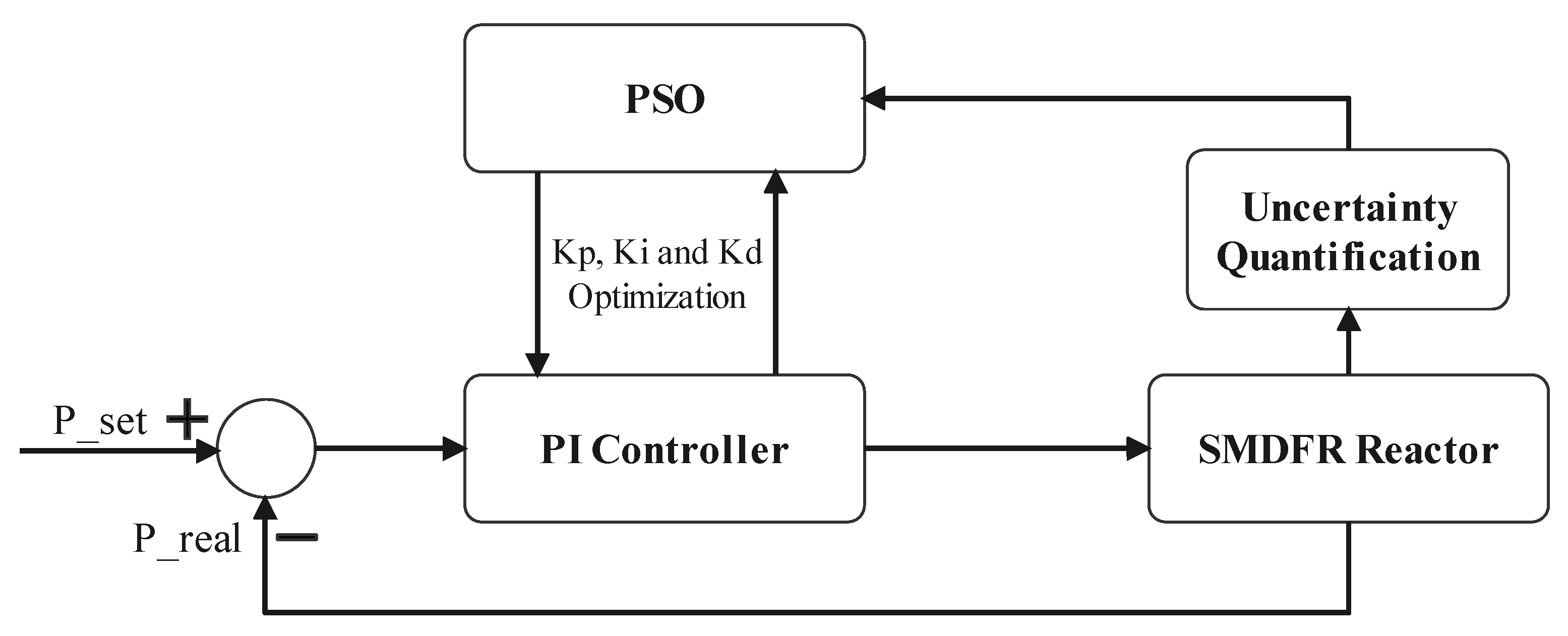
Figure 4.
Schematic of the balance of delayed neutron precursors.
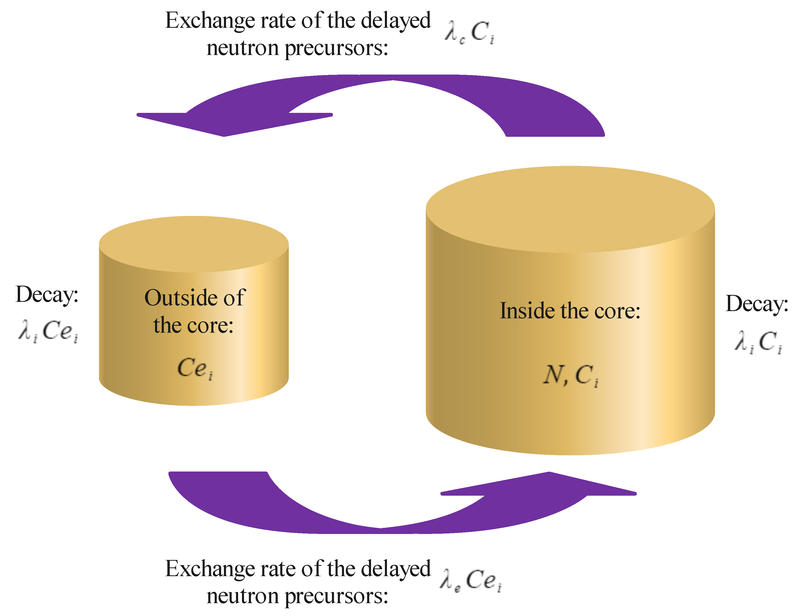
Figure 5.
Schematic of nodalization and energy balance.

Figure 6.
Flowchart of the design of the uncertainty-based control system.

Figure 7.
Verification of the 1D Matlab model against the 3D COMSOL model.

Figure 8.
System response of the insertion of reactivity: (a) insertion of reactivity at 100 pcm; (b) Insertion of reactivity at –100 pcm.
Figure 8.
System response of the insertion of reactivity: (a) insertion of reactivity at 100 pcm; (b) Insertion of reactivity at –100 pcm.

Figure 9.
System response of variation in inlet temperature: (a) inlet temperature increased by 20 C; (b) inlet temperature decreased by 20 C.
Figure 9.
System response of variation in inlet temperature: (a) inlet temperature increased by 20 C; (b) inlet temperature decreased by 20 C.

Figure 10.
System response of the variation in the coolant mass flow rate: (a) coolant mass flow rate increased by 10%; (b) coolant mass flow rate decreased by 10%.
Figure 10.
System response of the variation in the coolant mass flow rate: (a) coolant mass flow rate increased by 10%; (b) coolant mass flow rate decreased by 10%.
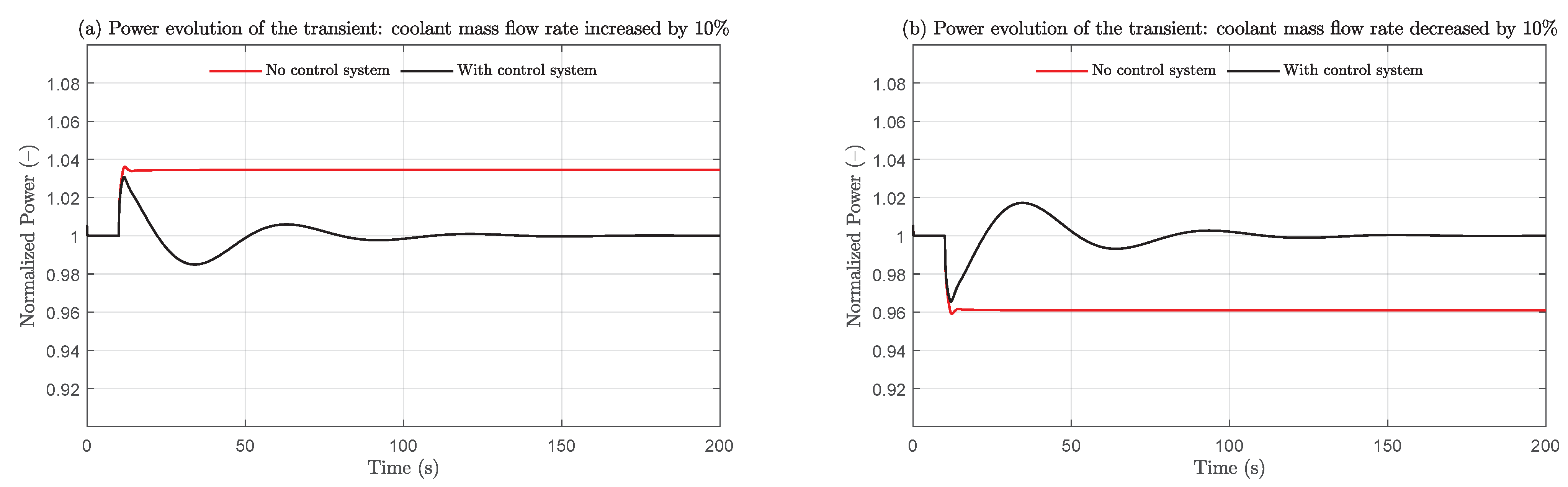
Figure 11.
Two benchmark cases: (a) step load change: 100% FP to 90% FP; (b) linear load change: 100% FP to 50% FP to 100% FP.
Figure 11.
Two benchmark cases: (a) step load change: 100% FP to 90% FP; (b) linear load change: 100% FP to 50% FP to 100% FP.

Figure 12.
Evolution of fitness value for the case of step load change.
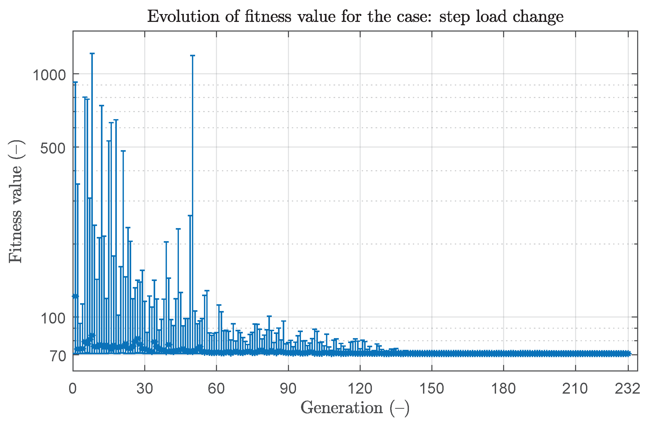
Figure 13.
Evolution of parameters for the case of step load change: (a) Kp; (b) Ki.

Figure 14.
Evolution of fitness value for the case of linear load change.

Figure 15.
Evolution of parameters for the case of linear load change: (a) Kp; (b) Ki.

Figure 16.
Introduced reactivity of the case of step load change.

Figure 17.
System responses of the case of step load change: (a) before optimization; (b) after optimization.
Figure 17.
System responses of the case of step load change: (a) before optimization; (b) after optimization.
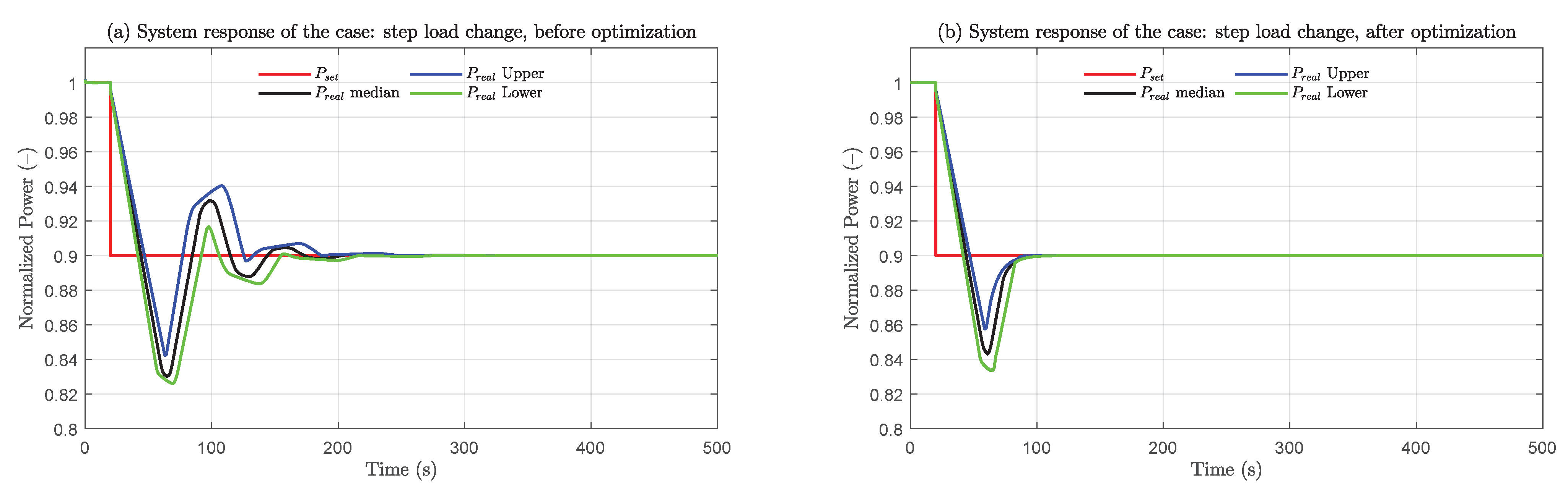
Figure 18.
Integral time-weighted absolute error of the case of step load change: (a) before optimization; (b) after optimization.
Figure 18.
Integral time-weighted absolute error of the case of step load change: (a) before optimization; (b) after optimization.
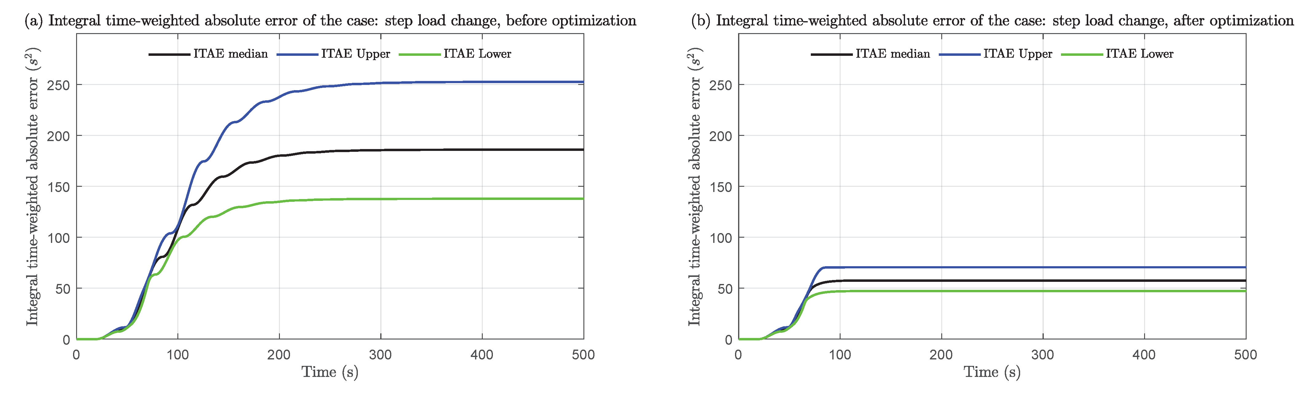
Figure 19.
System responses of the case of linear load change: (a) before optimization; (b) after optimization.
Figure 19.
System responses of the case of linear load change: (a) before optimization; (b) after optimization.

Figure 20.
Integral absolute error of the case of linear load change: (a) before optimization; (b) after optimization.
Figure 20.
Integral absolute error of the case of linear load change: (a) before optimization; (b) after optimization.
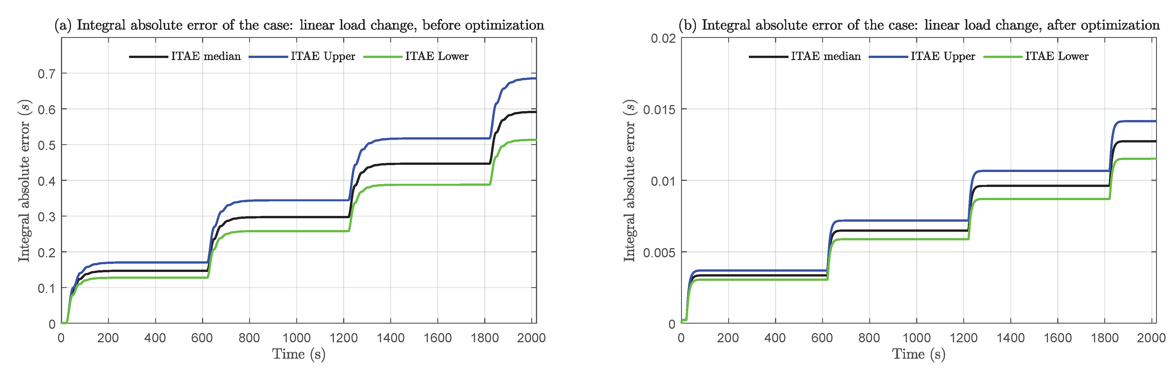
Figure 21.
Sensitivity analysis: (a) regression-based: SRC; (b) variance-based S1/ST.


Table 1.
SMDFR design parameters.
| Parameters | Values |
|---|---|
| Core zone D × H (m) | 0.95 × 2.0 |
| Distribution zone D × H (m) | 0.95 × 0.2 |
| Collection zone D × H (m) | 0.95 × 0.2 |
| Height of core (m) | 2.4 |
| Outer reflector diameter (m) | 1.25 |
| Tank D × H (m) | 1.65 × 3.4 |
| Number of fuel tubes | 1027 |
| Fuel pin pitch (m) | 0.025 |
| Outer/interior fuel tube diameter (m) | 0.008/0.007 |
| Outer/interior coolant tube diameter (m) | 0.005/0.004 |
| Mean linear power density (W/cm) | 609 |
| Fuel inlet/outlet temperature (K) | 1300/1300 |
| Coolant inlet/outlet temperature (K) | 973/1100 |
| Fuel inlet/in-core velocity (m/s) | 3/0.5225 |
| Coolant inlet/in-core velocity (m/s) | 5/1.3488 |
Table 2.
Neutronics data for the point kinetic model.
| Parameters | Value |
|---|---|
| ( ) | |
| ( ) | |
| ( ) | |
| 5.43 | |
| 10.0 | |
| 0.184 | |
| 0.1 | |
| ( ) | |
| ( ) |
Table 3.
Thermodynamics data.
| Parameters | Distribution Zone | Core Zone (1 from 10 Nodes) | Collection Zone |
|---|---|---|---|
| Fuel pipes (#) | - | - | 1027 |
| Coolant pipes (#) | 2166 | 2166 | - |
| 13.6 | 9.0 | 13.6 | |
| 10.9 | 10.3 | 10.9 | |
| 327.7 | 327.7 | 327.7 | |
| 5550.5 | 5550.5 | 5550.5 | |
| 307.7 | 116.4 | 307.7 | |
| 39.3 | 31.1 | 39.3 | |
| 219.9 | 770.5 | 219.9 | |
| 400 | 400 | 400 | |
| 690 | 690 | 690 | |
| 140.2 | 140.2 | 140.2 | |
| Heat taken by coolant (J) | 18,744,000 | 5,970,000 | 16,956,000 |
| 6546.0 | 4305.1 | 7629.5 | |
| 27,405.4 | 13,833.4 | 32,177.3 | |
| 1300.0 | - | - | |
| 973.0 | - | - |
Table 4.
Uncertain parameters.
| # | Parameters | Probability Density Function | Min. | Max. |
|---|---|---|---|---|
| 1 | Thermal power (factor) | Uniform | 0.98 | 1.02 |
| 2 | Temperature feedback coefficient of fuel (factor) | Uniform | 0.9 | 1.1 |
| 3 | Temperature feedback coefficient of coolant (factor) | Uniform | 0.9 | 1.1 |
| 4 | Mass flow rate of fuel (factor) | Uniform | 0.95 | 1.05 |
| 5 | Mass flow rate of coolant (factor) | Uniform | 0.95 | 1.05 |
| 6 | Heat capacity of fuel (factor) | Uniform | 0.95 | 1.05 |
| 7 | Heat capacity of coolant (factor) | Uniform | 0.95 | 1.05 |
| 8 | Heat transfer coefficient between fuel and wall (factor) | Uniform | 0.9 | 1.1 |
| 9 | Heat transfer coefficient between wall and coolant (factor) | Uniform | 0.9 | 1.1 |
| 10 | Fuel inlet temperature (additive) | Uniform | –2.2 | 2.2 |
| 11 | Coolant inlet temperature (additive) | Uniform | –2.2 | 2.2 |
Table 5.
Major parameters for the PSO process of step load change.
| Parameters | Value |
|---|---|
| Fitness function | |
| Number of variables | 2 |
| Constraints | none |
| Kp | 10~10,000 |
| Ki | 10~1000 |
| Population size | 20 |
| Generations | 300 |
| Social attraction | 1.25 |
Publisher’s Note: MDPI stays neutral with regard to jurisdictional claims in published maps and institutional affiliations. |
© 2021 by the authors. Licensee MDPI, Basel, Switzerland. This article is an open access article distributed under the terms and conditions of the Creative Commons Attribution (CC BY) license (https://creativecommons.org/licenses/by/4.0/).
Share and Cite
MDPI and ACS Style
Liu, C.; Luo, R.; Macián-Juan, R. A New Uncertainty-Based Control Scheme of the Small Modular Dual Fluid Reactor and Its Optimization. Energies 2021, 14, 6708. https://doi.org/10.3390/en14206708
AMA Style
Liu C, Luo R, Macián-Juan R. A New Uncertainty-Based Control Scheme of the Small Modular Dual Fluid Reactor and Its Optimization. Energies. 2021; 14(20):6708. https://doi.org/10.3390/en14206708
Chicago/Turabian StyleLiu, Chunyu, Run Luo, and Rafael Macián-Juan. 2021. "A New Uncertainty-Based Control Scheme of the Small Modular Dual Fluid Reactor and Its Optimization" Energies 14, no. 20: 6708. https://doi.org/10.3390/en14206708
Note that from the first issue of 2016, this journal uses article numbers instead of page numbers. See further details here.