Prediction of Electromagnetic Characteristics in Stator End Parts of a Turbo-Generator Based on MLP and SVR

Abstract

In order to study the multiple restricted factors and parameters of the eddy current loss of generator end structures, both the multi-layer perceptron (MLP) and support vector regression (SVR) are used to study and predict the mechanism of the synergistic effect of metal shield conductivity, relative permeability of clamping plates and structural characteristics of eddy current losses. Based on the eddy current losses of generator end structures under different metal shielding thicknesses and electromagnetic properties, the calculation accuracy of the MLP and SVR is compared. The prediction method gives an effective means for the complex design of the end region of the generator, which reduces the effort of the designers. It also promotes the design efficiency of the electrical generator.

1. Introduction

Due to the special nature of the end structure of turbo-generators, the distribution of magnetic flux leakage is complex. The distribution of eddy current loss is affected by many factors, such as the size, shape and physical properties of the end structure. The existing literature studies the influence of single factors on the electromagnetic loss of generator end structures and draws some basic research conclusions. Since the eddy current loss of generator end structures is affected by the conductivity, permeability and thickness of the structure, the relationship between these factors and the eddy current loss is difficult to display and record. Even if this corresponding function relationship makes sense to a certain extent, it may be a hypothetical one as a result of the ignorance of certain factors. The deviation analysis may be large and with a limited generalization ability of the obtained results.

Recently, scholars and researchers have performed extensive investigations on magnetic fields and eddy current issues of electrical machines. S. Utegenova et al. analyzed the magnetic issue of a wound-rotor motor by using an equivalent circuit method and introducing the principle of the magnetic equivalent circuit model [1]. J. Nam et al. proposed a new closed-path magnetic system. A mapping method was proposed to utilize the FEM and polynomial regression in order to analyze the magnetic field [2]. In [3], the impact of the leading degree on the eddy losses was analyzed. J. J. Perez-Loya et al. calculated the generator loss with a parallel path of the stator. Considering the unbalanced magnetic pull, both the currents of the damper bar and the circulating currents of stator winding were researched [4]. S. Kahourzade et al. conducted an electromagnetic analysis for a tapered axial flux PM machine. A new procedure of loss breakdown and efficiency estimation was introduced by both the experiment and the FEM [5]. In [6], some laws were proposed for using analytical methods to analyze eddy current losses of AC generators. J. L. Risti’c-Djurovi’ et al. introduced a new method to add extra stator windings to enlarge the length of the variation along a test volume direction [7]. In [8], the circulating currents of the double-stator Roebel bars were calculated by using several models. The calculation results and test data were compared, and the advantage of each model was discussed. J. Lee et al. proposed a calculation method to include the additional losses, which is not considered in many cases [9]. In [10], A. Tessarolo et al. conducted research on the eddy currents by the time-harmonic FEA. In some methods, they are alternative. In [11], the influence of the main deformation of the shape and size of the winding section of the circular solenoid on the magnetic field’s distribution and uniformity was studied. Y. Kwon et al. used two simplified nonlinear magnetic equivalent circuit models to analyze the magnetic field capability caused by the change in design parameters of the new soft magnetic composite prototype as compared with the basic model prototype [12]. In [13], a multi-objective optimization design for a non-core PM synchronous motor was introduced. By solving two Laplace equations, both the 3D performance analysis and the magnetic field distribution were obtained under open circuit conditions. In [14], Vraisanen et al. proposed a time harmonic model, which can be used to deal with multi-layer cylindrical rotors. In order to consider the influence of the stator slot on eddy current loss, the calculation model was linked to a finite element solution by covering the stator. M. Z. Youssef et al. introduced a new electromagnetic analysis method by optimizing the cost of the electromagnetic system based on mathematical analysis [15]. In [16], a numerical model of the magnetic bearing was proposed. The 3D magnetic field’s distribution between the stator and the rotor was calculated. In addition, the magnetic forces of the hybrid magnetic bearing system were studied under different stator currents. P. Hekmati et al. established the magnetic analytical models for different rotor structures of electrical machines. The electromagnetic parameters of both stator and rotor sides were obtained [17]. G. G. Sotelo et al. suggested a new design method for a motor. By changing the load condition, the proposed motor can operate both under a synchronous state and a hysteresis state [18]. S. G. Min et al. presented a novel analytical solution to obtain the best electromagnetic performances of concentrated windings of the stator and of the permanent magnet machines [19]. J. Lee et al. conducted an electromagnetic analysis for a PM sensor. Both the position and structure of the PM Hall sensor were considered. The proposed magnetic equivalent circuit model gained a fast calculation result [20]. P. R. Eckert et al. developed a model for obtaining the flux distribution and the stator voltage. The method was validated by an experiment of an actual prototype [21]. In [22], a support vector machine (SVM) was used to classify and evaluate induction motor faults. The calculation results showed that, compared with the other two machine learning algorithms, the SVM calculation results were more accurate. The fuzzy C-Means machine learning algorithm was used to analyze the influence of the flux sensor position on the automatic classification. The results proved the potential of the method for its future incorporation into autonomous condition monitoring systems that can be satisfactorily applied to determine the health of these machines [23]. In [24], the linear prediction coefficients and mel frequency cepstral coefficients were extracted from the machine sound to develop. Machine learning (ML) models were created to monitor and identify the malfunctioning machines based on the operating sound. The experimental results showed the performance of ML models for the machine sound recorded, with different signal-to-noise ratio levels for normal and abnormal operations.

In this paper, a mathematical model of a 3D magnetic field in the complex end domain of the generator end is established by a time-step FEM. A neural network and support vector regression are used to study and predict the mechanism of the synergistic effect of the metal shield conductivity, relative permeability of clamping plates and structural characteristics of the eddy current loss of end structures. The prediction accuracy of the MLP and SVR are compared. This research provides an effective means for the complex design of generator end regions, which reduces the effort of designers. In addition, it promotes the design efficiency of the electrical generator.

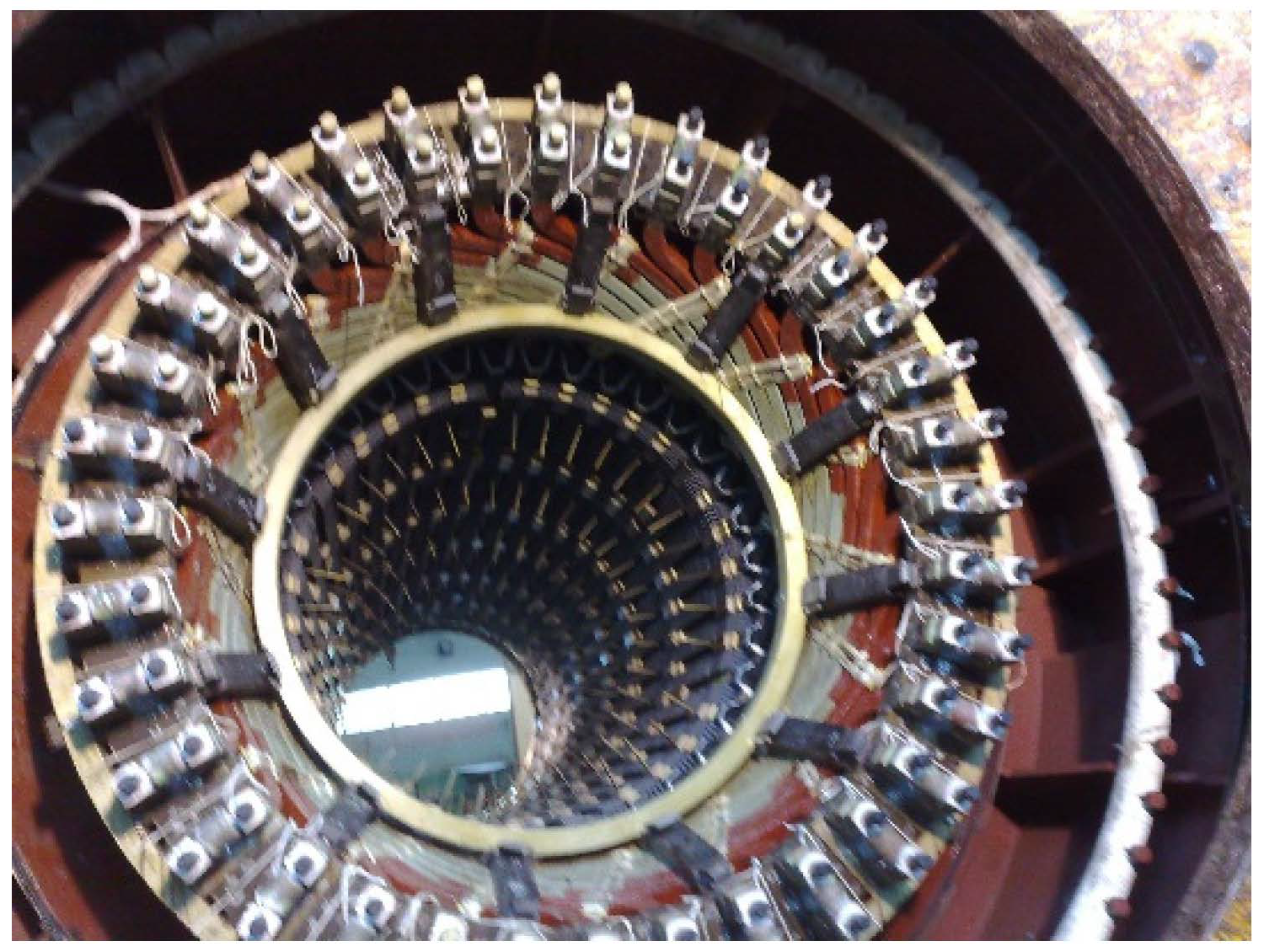
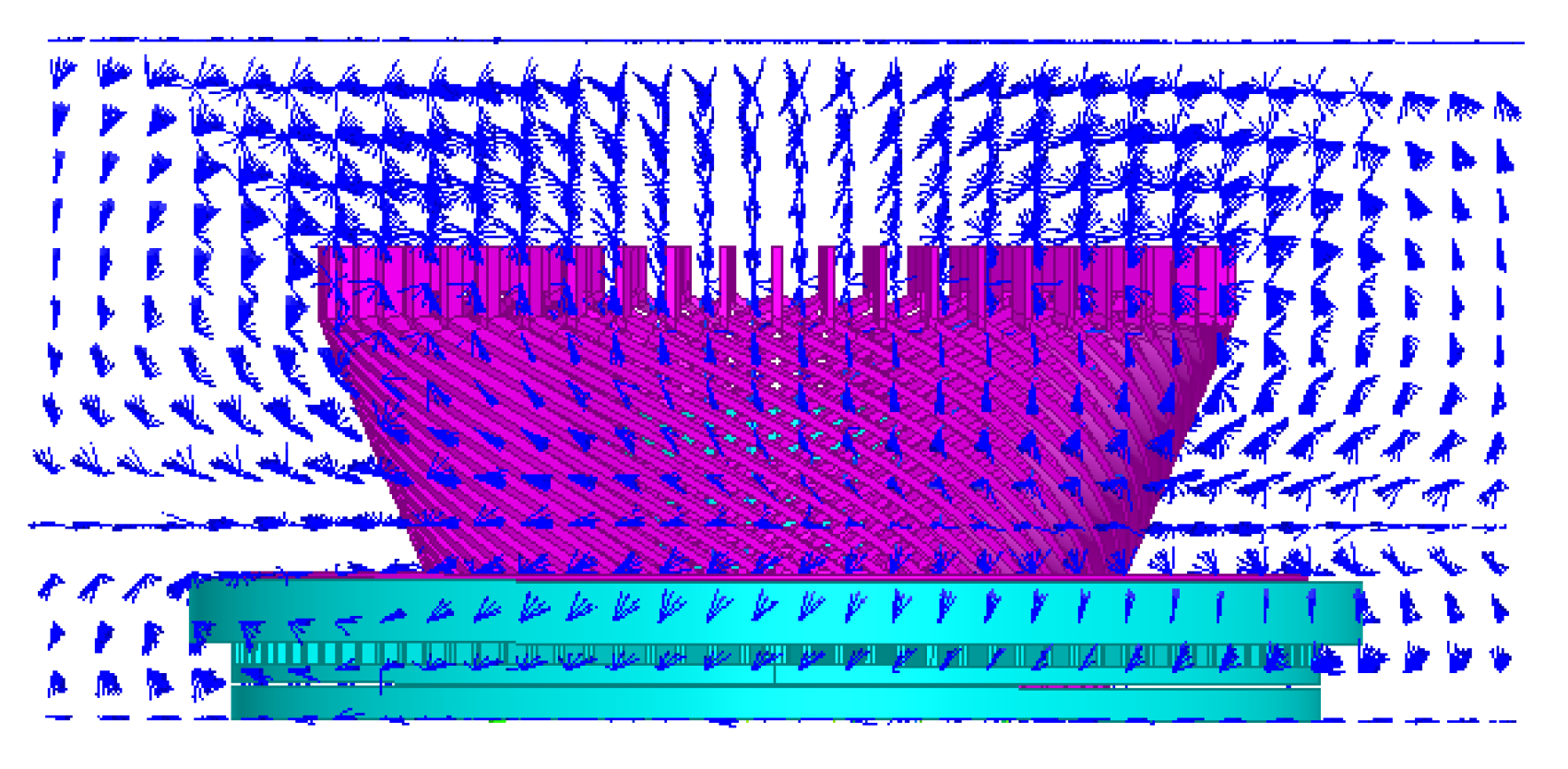
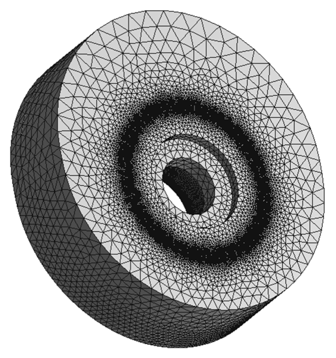
2. 3D Electromagnetic Field Analysis

The stator end windings have an involute structure. There are many different metal structures, such as a finger plate, copper screen and clamping plate.

Table 1. Basic parameters.

Parameters	Values
Power	330 MW
Stator voltage	20 kV
Stator current	11.2 kA
Speed	3000 rpm
Rated efficiency	98.8%
Cooling medium	Hydrogen

gives the basic parameters of this 330 MW hydrogen turbo-generator, which is used to calculate the flux of the end domain.

Figure 1 shows the end structure of a hydrogen-cooled turbo-generator prototype. Based on the actual size of the generator end domain, a 3D electromagnetic field model was established, which is shown in Figure 2. Because the generator pole number is small, both the end winding span and the total end domain space are relatively large.

In order to truly reflect the actual results, the end domain of the 330 MW generator was established based on the actual shape and dimensions of the prototype. The whole solution domain Ω contains the eddy current domain V₁ and the non-eddy current domain V₂.

Figure 3 shows the solution domain of the 330 million W water–hydrogen–hydrogen-cooling turbo-generator. The mathematical model contains vector potential T and the scalar potential Ψ. The solution formulas are shown in (1)–(5) [25].

$$\{\begin{array}{l}\nabla \times \rho \nabla \times \mathit{T}-\nabla \rho \nabla ·\mathit{T}+\frac{\partial \mu (\mathit{T}-\nabla \psi )}{\partial t}+\frac{\partial \mu {\mathit{H}}_s}{\partial t}=0\\ \nabla ·\mu (\mathit{T}-\nabla \psi )=-\nabla ·\mu {\mathit{H}}_s\end{array}$$

(1)

$$\nabla ·\mu \nabla \psi =\nabla ·\mu {\mathit{H}}_s \mathrm{in} V_2$$

(2)

where

$${\mathit{H}}_s=\frac{1}{4\pi }{\displaystyle {\int }_{{\Omega }_s}\frac{{\mathit{J}}_s\times \mathit{r}}{r^3}}\mathrm{d}\Omega$$

(3)

Boundary conditions:

$$\{\begin{array}{l}{\frac{\partial \psi }{\partial n}|}_{S_1,S_2}=0\\ {\psi |}_{S_3}={\psi }_0\end{array}$$

(4)

The initial conditions:

$$\{\begin{array}{l}{T|}_{V_1}=T_0\\ {\psi |}_{\Omega }={\psi }_0\end{array}$$

(5)

where ${\mathit{J}}_s$ is the source current density in the windings(in A/m²), $\mu$ is the permeability(in H/m), $\rho$ is the resistivity (in Ω·m), $T_0$ is the electric vector potential at the initial time, ${\psi }_0$ is the scalar magnetic potential at the initial time, $t$ is the time(in s), and $n$ is the normal vector of the surface.

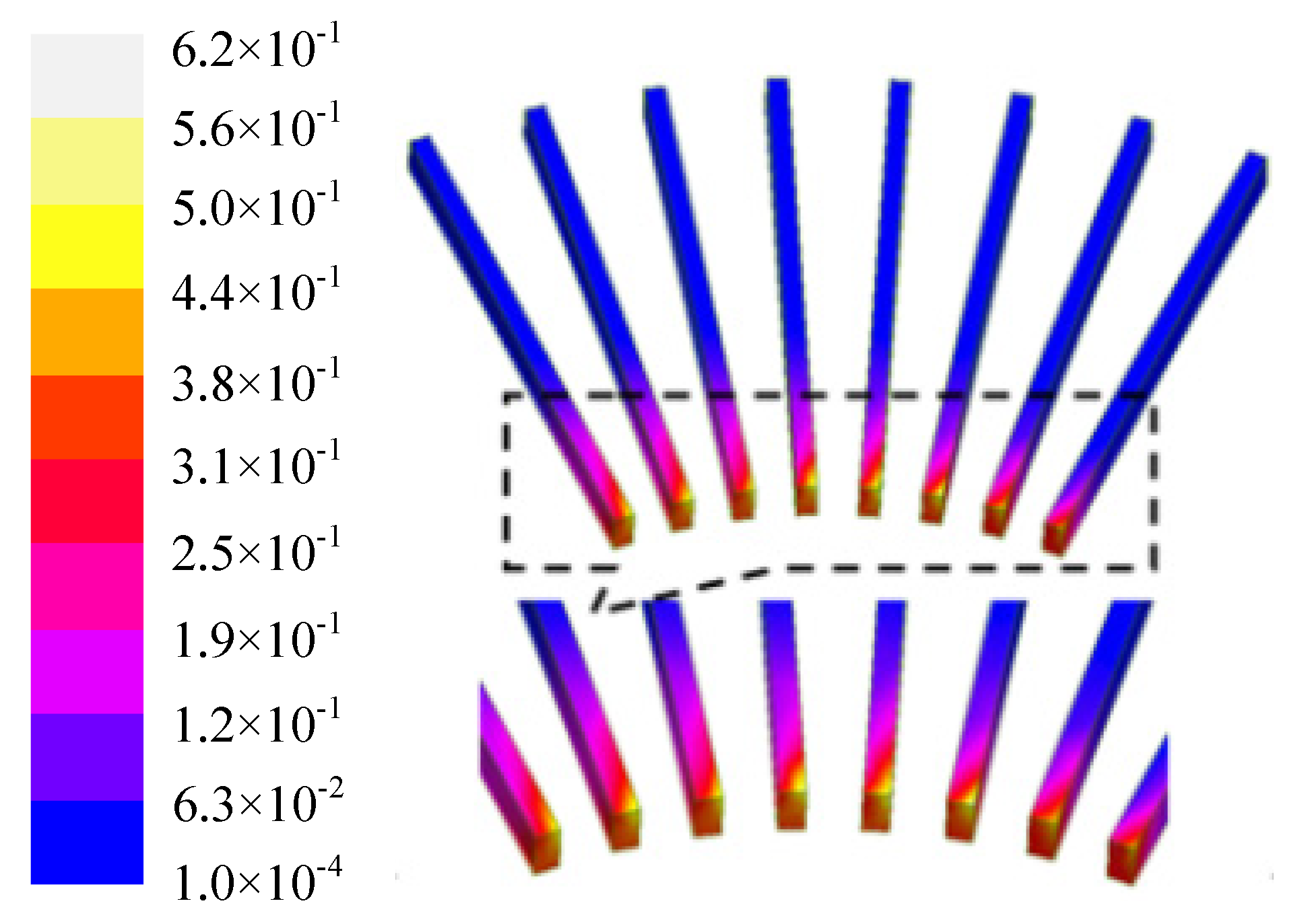
3. Electromagnetic Losses of Metal Parts

3.1. Electromagnetic Loss Calculation and Analysis

Figure 4 gives the distribution of the leakage flux field in the end domain of the turbo-generator. This shows that the magnetic flux leakage passes around the armature windings. The magnetic flux leakage is essentially parallel to the outer surface of the copper screen.

Figure 5 shows the eddy current distribution in the copper screen. The yellow arrow shows the path of the eddy current in the copper screen. The distribution of the eddy current density indicates that the copper screen is essential for preventing the intrusion of the end leakage flux into the clamping plate.

Figure 6 gives the value of the magnetic flux density of the finger plates. The magnetic flux density is high at the front of the finger plates. The value reduces from the front parts to the back parts. In the end domain, the eddy current losses are not only impacted by the radial component of the total flux; due to the complex structure, the axial component of the flux also exists in this domain.

The eddy current loss of metal structures is calculate by (6)

$$P_e=\frac{1}{T_c}{\displaystyle \underset{T_c}{\int }{\displaystyle \sum _{i=1}^k{J}_e^2{\mathsf{\Delta }}_e}{\sigma }_r^{-1}\mathrm{d}t}$$

(6)

where $P_e$ is losses of the element (in W), $J_e$ is the eddy current density (in A/m²), ${\Delta }_e$ is the element volume (in m³), ${\sigma }_r$ is the metal component conductivity (in S/m), T_c is the period (in s), k is the total element number in volume, and e is the element number.

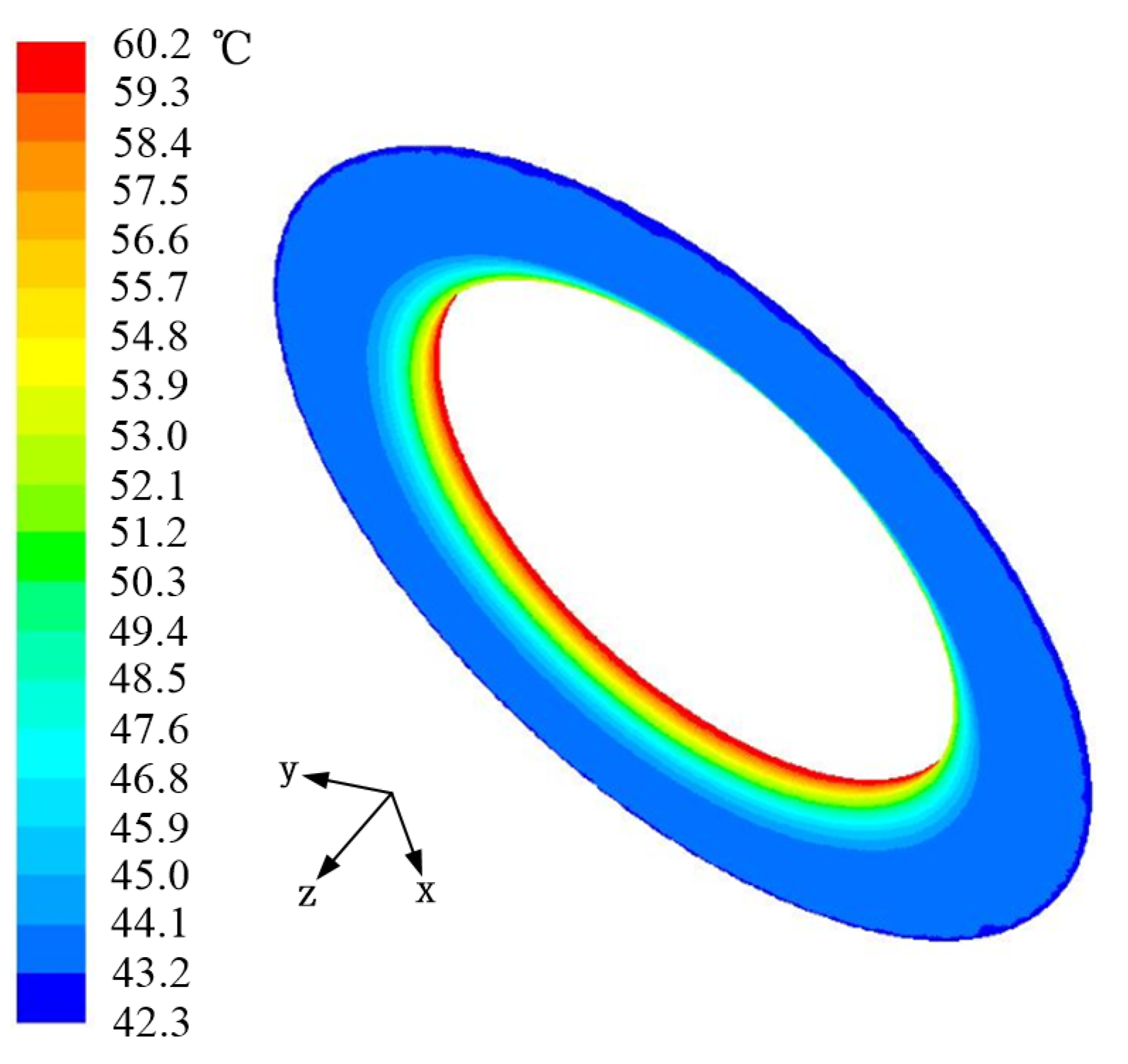
3.2. Verification for Electromagnetic Loss Calculation by Thermal Test

Using the results of the electromagnetic losses as heat sources, the temperature field of the end domain can be calculated [26]. The fluid–solid coupled model is given in Figure 7. Figure 8 gives the mesh results of the solution domain. The total number of mesh elements is 7,932,399.

Figure 9 gives the temperature of the copper screen.

Table 2. Test values.

	Position M	Position N	Position P
Temperature (°C)	74.3	63.6	56.9

shows the measured values of the temperature. Figure 10 and Figure 11 give the locations of the temperature sensors and the copper screen used for the test.

The end structures may not be absolutely symmetric, such as the distance between the adjacent windings and the distance between the adjacent water pipes in the stator windings. These factors could cause the velocity distribution of the cooling medium to be asymmetric. The deformation of the end structures could also result in asymmetric distribution of loss. The measured results are different values at different positions, which may be caused by these asymmetric factors. For the simulation results, the highest temperature of the copper screen is 60.2 °C. The average temperature of the copper screen is 57.3 °C.

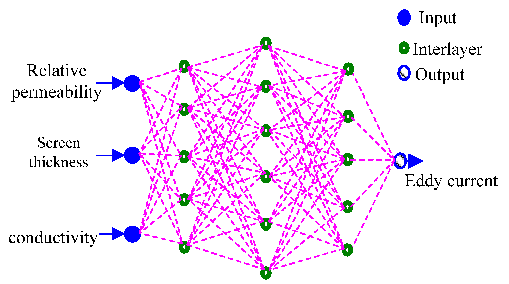
4. Prediction and Result Analysis Using Multi-Layer Perceptron

4.1. Prediction and Analysis Based on Multi-Layer Perceptron

In order to research the collaborative impact of multiple factors on the eddy current losses of end structures, the back propagate neural network (BPNN) model is established to study the known samples that are calculated by the FEM. The input nodes are the multi-factors, which have the thickness of a metal screen, the conduction characteristics of a metal screen and the permeability performance of a clamping plate. These factors are the elements of the input vector of the BPNN model. The output vector is the total eddy current of the end structures. The BPNN model is shown in Figure 12. To improve the prediction accuracy of forecasting samples and the generalization ability of the BPNN model, the middle hidden layer has multiple layers. In this paper, the hidden layer of the BPNN model has three layers, which are 5, 6, and 5.

The input vector A = (ur, thk, sim), the output vector Y = (loss).

where ur is the relative permeability of the clamping plate, thk is the thickness of the copper screen, sim is the conductivity of the metal screen, and loss is the total eddy current losses of end structures.

(1)

In the process of information forward propagation, if $a_i^{(1)}=x_i$ is the input value (activation value) of layer 1 neurons, the activation value of the next layer is [27]:

$$\{\begin{array}{l}{a}_j^{(1)}=x_i\hfill \\ a_j^{(l+1)}=f\left(z_j^{(l+1)}\right)\hfill \\ z_j^{(l+1)}={\displaystyle \sum _{i=1}^n}{W}_{ji}^{(l)}{a}_i^{(l)}{b}_j^{(l)}\hfill \end{array}$$

(7)

where $x_i$ is the input value of neuron i node data of the first layer of sample data; $a_i^{(l)}$ represents the output value of the i-th node of the l-th layer; and $z_j^{(l)}$ represents the activation value of node j of layer 1. $W_{ji}^{(l)}$ is the connection weight parameter between the i-th node of layer l and the j-th node of layer l + 1; $b_j^{(l)}$ is the intercept term of node j on layer l + 1. f is the sigmoid activation function, and the expression is $\phi (x)=\frac{1}{1+e^{-x}}$.

(2)

Error back propagation process [28]

$$C(W,b)=\frac{1}{2}\sum _{i\in \mathrm{outputs}}\Vert y_i-a_i{}^2\Vert$$

(8)

where $y_i$ is the true value of node i traffic of the sample data output layer; $a_i$ is the flow output value of node i in the sample data output layer.

(3)

Determination of optimization objectives

W (weight) and b (bias) minimize the loss function C(W,b), and the flow prediction value output by the model will be closer to the real value. The iterative formula of W and b is as follows [29]:

$$\{\begin{array}{l}{W}_{ji}^{(l)}=W_{ji}^{(l)}-\alpha \frac{\partial C(W,b)}{\partial W_{ji}^{(l)}}\hfill \\ b_j^{(l)}=b_j^{(l)}-\alpha \frac{\partial C(W,b)}{\partial b_j^{(l)}}\hfill \end{array}$$

(9)

where $\alpha$ is the learning rate, and the value range is (0, 1).

4.2. Deviation Analysis and Generalization Ability Based on Multi-Layer Perceptron Prediction

Table 3. The training sample sets of eddy current losses.

Sample	Relative Permeability	Thickness (mm)	Conductivity (S/m)	Eddy Current Loss (kW)
1	1	12	46,082,949	25.42
2	10	12	46,082,949	24.40
3	20	12	46,082,949	24.01
4	30	12	46,082,949	23.95
5	40	12	46,082,949	24.01
6	50	12	46,082,949	24.09
7	1	12	46,082,949	25.42
8	1	14	46,082,949	22.80
9	1	16	46,082,949	22.12
10	1	18	46,082,949	21.24
11	1	20	46,082,949	20.90
12	1	22	46,082,949	20.33
13	1	12	6,418,485	53.79
14	40	12	6,418,485	37.86
15	100	12	6,418,485	26.22

shows the training sample sets of the total eddy current losses of end structures. Before predicting the eddy current losses of test sample sets, data training and learning should be conducted for the training sample sets.

The highly precise learning results are gained through the training samples of the eddy current loss of each structure based on the BPNN with a middle layer of the 5–6–5 type, as shown above. Figure 13 gives the learning results of the eddy current losses of each of the structures based on the BPNN with a middle layer of the 5–6–5 type. From Figure 13, we learn that the variation trend of the FEM and MLP is the same, and the eddy current loss is the largest around the seventh sampling point.

Table 4. Predicted eddy current losses of the test sample set (Kw).

Relative Permeability	Thickness (mm)	Conductivity (S/m)	Losses
			FEM	MLP
1	12	28,589,902	32.57	32.77
1	20	28,589,902	28.02	27.99
2	12	46,082,949	25.06	25.07
4	12	46,082,949	24.99	24.93
8	12	46,082,949	24.57	24.67

gives a comparison between the predicted results of the test sample and the calculated results by the finite element method. It is shown that even if the electrical conductivity of metal aluminum material is not provided in the training sample, the MLP predicts that the loss value of the end structure parts is close to the calculated values by the finite element method when the end of generator is shielded by metal aluminum.

When the hidden layers are changed to two layers, the predicted result of (32.77, 27.99, 25.07, 24.93, 24.67) is changed to (33.81, 30.00, 25.22, 25.02, 24.67). It shows that, for the prediction loss results of the end structure parts of a turbo-generator by the BPNN, the deviation between the eddy current loss of end structure parts by the MLP and its calculated results by the finite element method decreases with the increase in hidden layers of the neural network.

5. Prediction and Results Analysis by SVR

5.1. Mathematical Principle of Support Vector Regression

Support vector regression (SVR) belongs to the category of statistics, and the idea is to use classification as the leading factor. SVR has the characteristics of low risk, which avoid the defects of blind training, over-learning and entering the minimum region of traditional prediction methods. SVR is suitable for the data mining of small sample sets, and its generalization ability is strong. SVR is often the first choice in order to study small sample data. This data-mining model maps high-dimensional space to low-dimensional space by selecting the kernel function, which makes the problem less complex. During this period, it does not increase the difficulty of calculation and effectively avoids the issue of dimension. Therefore, SVR is widely used in predicting engineering problems [30,31,32,33,34,35].

Let the sample set be $\left\{(x_i,y_i)|x_i\in R^n;y_i\in \left\{-1,+1\right\},i=1,\dots ,I\right\}$, and find an optimal hyperplane that has two types of points labeled +1 and −1 that are not only separated but also have the largest separation interval.

Linear separation can be achieved in n-dimensional Euclidean space; that is, there is a hyperplane that divides the sample set on both sides according to the labels −1 and +1. Since the mathematical expression of the hyperplane in n-dimensional Euclidean space is a linear equation $<w,x>+b=0$, this means that among them, $w$ is a coefficient vector, $x$ is a n-dimensional variable, $<w,x>$ is an inner product, and $b$ is a constant. The distance from point $x_i$ to hyperplane $L$ in space is denoted as $d(x_i,L)=\frac{|<w,x_i>+b|}{\left|\right|w\left|\right|}$. For maximization, $d(x_i,H)$ is equivalent to $\frac{1}{2}\left|\right|w|{|}^2$ minimum. Next, we obtain an extreme value problem under the following constraints.

$$\{\begin{array}{l}\min \frac{1}{2}\left|\right|w|{|}^2\\ y_i(<w,x_i>+b)\ge 1,i=1,2,\dots ,I\end{array}$$

(10)

By introducing Lagrange multiplier $\alpha =({\alpha }_1,{\alpha }_2,\dots ,{\alpha }_I)$, we can solve the equation about the parameter by (11).

$$Q(\alpha )={\displaystyle \sum _{i=1}^I{\alpha }_i-\frac{1}{2}}{\displaystyle \sum _{i,j=1}^I{\alpha }_i}{\alpha }_j{y}_i{y}_j<x_i,x_j>$$

(11)

The above formula is called the Lagrange dual function, and its constraint is expressed as (12).

$${\displaystyle \sum _{i,j=1}^I{\alpha }_i}{y}_i=0,{\alpha }_i\ge 0,i=1,2,\dots ,I$$

(12)

Under this constraint, if $\alpha$ makes $Q(\alpha )$ reach the maximum value, there are many ${\alpha }_i$ whose values are 0. However, the sample $x_i$ corresponds to ${\alpha }_i$, which is not 0 and is the support vector.

When linear separation cannot be achieved in the input space, it is assumed that non-linear mapping $\varphi$ is found. It can map the sample set that is expressed as $\left\{(x_i,y_i)|x_i\in R^n; y_i\in \left\{-1,+1\right\},i=1,\dots ,I\right\}$ into the high-dimensional feature space $H$.

Presently, we consider the linear classification of the set $\left\{(\varphi (x_i),y_i)|x_i\in R^n; y_i\in \left\{-1,+1\right\},i=1,\dots ,I\right\}$ in $H$ by constructing a hyperplane in $H$. Its weight coefficient $w$ satisfies similar extreme value problems. Since exceptions are allowed in some areas, slack terms can be introduced, that is, rewritten as:

$$\{\begin{array}{l}\min \frac{1}{2}{||w||}^2+C{\displaystyle \sum _{i=1}^L{\xi }_i}\\ y_i(<w,x_i>+b)\ge 1-{\xi }_i,{\xi }_i\ge 0,i=1,2,\dots ,I\end{array}$$

(13)

A classification problem is an extreme case, but it is very useful. Let $\{x_i|x_i\in R^n,i=1,\dots ,I\}$ be a finite observation point in space $R^n$. Find the smallest sphere containing these points with $a$ as the center and $R$ as the radius. Therefore, a classification is the best method for finding the minimum envelope surface of a compound component. Exactly as above, let $\varphi$ be the embedded mapping derived from a kernel function $K(x,s)$ from the input space to the feature space, and finally we understand the quadratic programming problem.

$$\{\begin{array}{l}{\min }_{\alpha }\frac{1}{2}\alpha \prime D\alpha +c\prime \alpha \\ y\prime \alpha =0,0\le \alpha ={({\alpha }_1,\dots {\alpha }_I)}^T\le A={(C,\dots ,C)}^T\end{array}$$

(14)

where $y={(y_1,\dots ,y_I)}^T$, $c={(-1,\dots ,-1)}^T$, and $D={(K(x_i,x_j)y_i{y}_j)}_{1\le i,j\le I}$ are matrixes. $K(x,s)$ is a kernel function. Then,

$$f(x)=K(x,x)-2{\displaystyle \sum _{i=1}^L{\alpha }_{i}K(x,x_i)+{\displaystyle \sum _{j=1}^L{\displaystyle \sum _{i=1}^L{\alpha }_i{\alpha }_j}}}K(x_i,x_j)$$

(15)

where all points satisfy the relationship with $f(x)\le R^2$. The parameter $C$ controls the number of points that fall outside the ball. The interval of change is $1/L<C<1$.

5.2. Prediction of Eddy Current Loss Based on SVR

According to the prediction principle of SVR, the mathematical prediction model of the eddy current loss of generator end structures with multiple factors, such as metal shielding thickness, metal shielding conductivity and relative permeability of clamping plates, is constructed. The training sample set above is studied again, and the test sample set is predicted. Figure 14 shows the learning result of the eddy current losses of turbo-generators based on SVR. From Figure 14 displaying the learning results of eddy current loss based on SVR, it can be observed that there are deviations in individual points of the learning results, but the deviations in the overall learning results are small.

Table 5. Predictive eddy current losses in the test sample based on SVR.

Relative Permeability	Thickness (mm)	Conductivity (S/m)	Losses (kW)
			FEM	SVR
1	12	28,589,902	32.57	31.72
1	20	28,589,902	28.02	27.20
2	12	46,082,949	25.06	25.32
4	12	46,082,949	24.99	25.22
8	12	46,082,949	24.57	25.03

gives the prediction results of the loss of generator end structures in the test samples based on SVR. It is not difficult to see that the eddy current loss has a high prediction accuracy and strong generalization ability based on SVR. The deviation of learning results of individual elements in the training set does not affect the accurate prediction of eddy current loss of the test samples from SVR.

6. Conclusions

In this paper, in order to study the multiple restricted factors of the eddy current loss of generator end structures, a mathematical model of the 3D electromagnetic field in the complex end domain is established by the time-step FEM. Both the neural network and the support vector regression are used to study and predict the mechanism of the synergistic effect of metal shield conductivity, relative permeability of clamping plates and structural characteristics on the eddy current loss of end structures. The different prediction types are compared, and the accuracy of the prediction of loss results is studied.

(1)

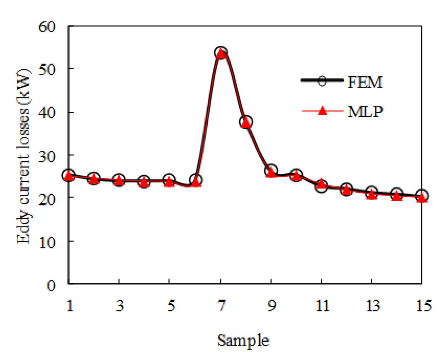
The learning results and predicted eddy current loss of the test samples fit well with the numerical calculation from the FEM. This shows that even if the electrical conductivity of metal aluminum material is not provided in the training sample, the MLP can predict that the loss value of end structure parts is close to the calculated values by the finite element method when the end of the generator is shielded by metal aluminum. When the relative permeability is 1, the conductivity is 28,589,902 S/m, and the thickness increases from 12 to 20 mm, the eddy current loss obtained by the FEM is reduced by 14%, and the eddy current loss obtained by the MLP is reduced by 14.6%. When the relative permeability increases from 2 to 4, the conductivity is 46,082,949 S/m and the thickness is 12 mm, the eddy current loss obtained by the FEM is reduced from 25.06 to 24.99 kW, and the eddy current loss obtained by the MLP is reduced from 25.07 to 24.93 kW. When the relative permeability increases from 4 to 8, the conductivity is 46,082,949 S/m and the thickness is 12 mm, the eddy current loss results obtained by the FEM and MLP are also reduced.

(2)

For the prediction results of the eddy current loss of end structure parts of the turbo-generator by the BPNN, the deviation between the eddy current loss of end structure parts by the MLP and the eddy current loss gained by the FEM decreases with the increase in hidden layers of the neural network.

(3)

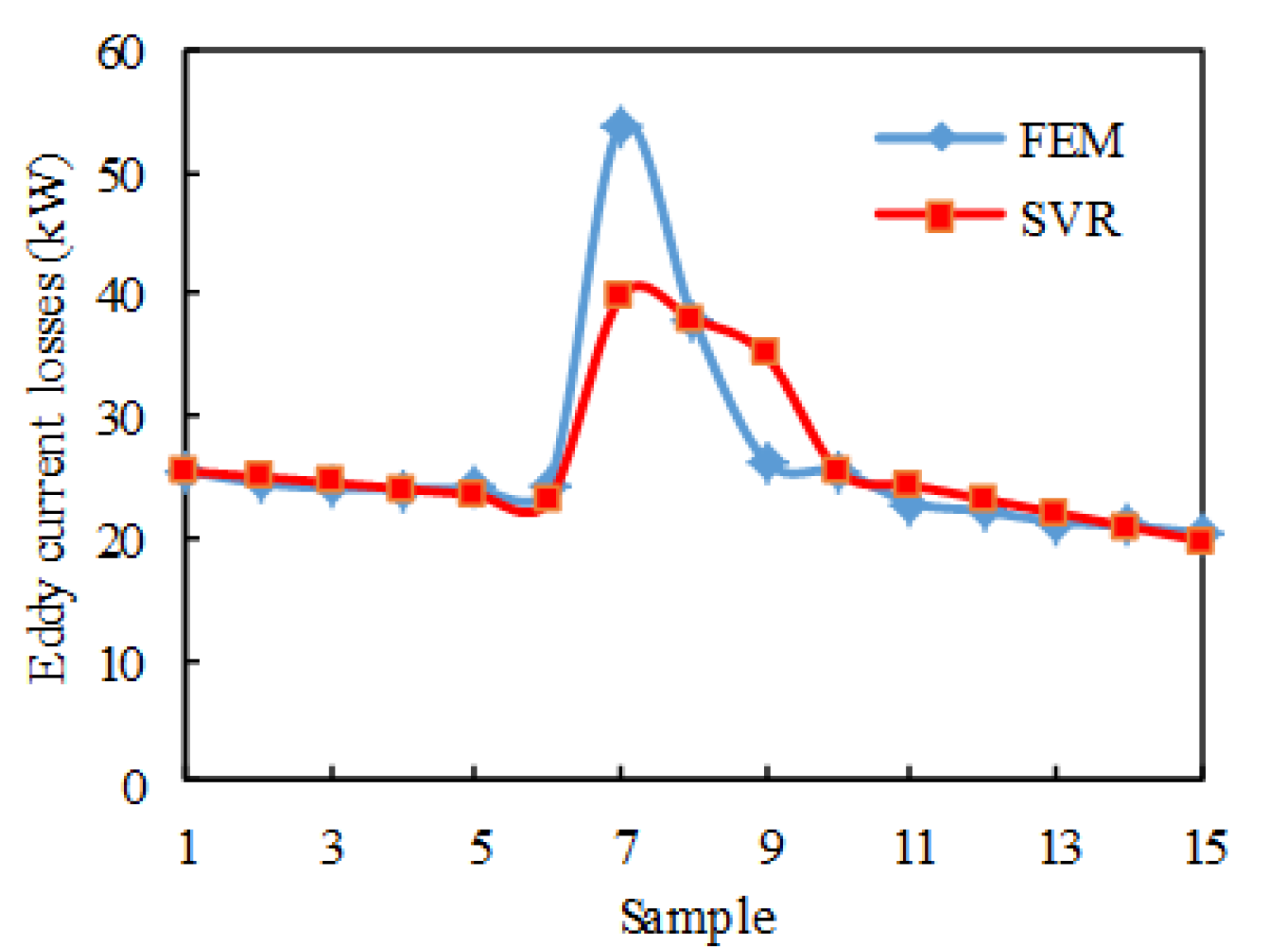
From the results of the eddy current loss learning based on SVR, there are deviations in individual points of the learning results, but the deviations in the overall learning results are small. Eddy current loss has a high prediction accuracy and strong generalization ability based on SVR. The deviation of learning results of individual elements in the training sets does not affect the accurate prediction results of the eddy current loss of the test samples based on SVR.

This method gives an effective means for the complex design of the end region of the generator, which reduces the effort of designers. It also promotes the design efficiency of the electrical generator.

In future studies, a large data sample for a three-dimensional mathematical model of the end transient electromagnetic field of a turbine generator will be constructed, and the effect of the end magnetic leakage on the loss of the structural parts will be studied separately in combination with deep learning. In addition, big data samples with more influencing factors will be constructed, and models with more layers will be applied to further improve the accuracy of the prediction model.

References

1. Utegenova, S.; Dubas, F.; Jamot, M.; Glises, R.; Truffart, B.; Mariotto, D.; Lagonotte, P.; Desevaux, P.; Utegenova, S.; Desevaux, P. An Investigation Into the Coupling of Magnetic and Thermal Analysis for a Wound-Rotor Synchronous Machine. IEEE Trans. Ind. Electron. 2017, 65, 3406–3416. [Google Scholar] [CrossRef]
2. Nam, J.; Lee, W.; Jung, E.; Jang, G. Magnetic Navigation System Utilizing a Closed Magnetic Circuit to Maximize Magnetic Field and a Mapping Method to Precisely Control Magnetic Field in Real Tim. IEEE Trans. Ind. Electron. 2018, 65, 5673–5681. [Google Scholar] [CrossRef]
3. Wang, L.; Li, W. Influence of underexcitation operation on electromagnetic loss in the end metal parts and stator step packets of a turbogenerator. IEEE Trans. Energy Convers. 2014, 29, 748–757. [Google Scholar] [CrossRef]
4. Perez-Loya, J.J.; Abrahamsson, C.J.D.; Lundin, U.; Abrahamsson, J. Electromagnetic Losses in Synchronous Machines During Active Compensation of Unbalanced Magnetic Pull. IEEE Trans. Ind. Electron. 2018, 66, 124–131. [Google Scholar] [CrossRef]
5. Kahourzade, S.; Ertugrul, N.; Soong, W.L. Loss Analysis and Efficiency Improvement of an Axial-Flux PM Amorphous Magnetic Material Machine. IEEE Trans. Ind. Electron. 2018, 65, 5376–5383. [Google Scholar] [CrossRef]
6. Drubel, O.; Stoll, R.L. Comparison between analytical and numerical methods of calculating tooth ripple losses in salient pole synchronous machines. IEEE Trans. Energy Convers. 2001, 16, 61–67. [Google Scholar] [CrossRef]
7. Ristić-Djurović, J.L.; Gajić, S.S.; Ilić, A.Ž. Design and Optimization of Electromagnets for Biomedical Experiments with Static Magnetic and ELF Electromagnetic Fields. IEEE Trans. Ind. Electron. 2018, 65, 4991–5000. [Google Scholar] [CrossRef]
8. Haldemann, J. Transpositions in Stator Bars of Large Turbogenerators. IEEE Trans. Energy Convers. 2004, 19, 553–560. [Google Scholar] [CrossRef]
9. Jun, H.-W.; Lee, J.-W.; Yoon, G.-H.; Lee, J. Optimal Design of the PMSM Retaining Plate with 3D Barrier Structure and Eddy-Current Loss-Reduction Effect. IEEE Trans. Ind. Electron. 2017, 65, 1808–1818. [Google Scholar] [CrossRef]
10. Tessarolo, A.; Agnolet, F.; Luise, F.; Mezzarobba, M. Use of Time-Harmonic Finite-Element Analysis to Compute Stator Winding Eddy-Current Losses Due to Rotor Motion in Surface Permanent-Magnet Machines. IEEE Trans. Energy Convers. 2012, 27, 670–679. [Google Scholar] [CrossRef]
11. Beiranvand, R. Effects of the Winding Cross-Section Shape on the Magnetic Field Uniformity of the High Field Circular Helmholtz Coil Systems. IEEE Trans. Ind. Electron. 2017, 64, 7120–7131. [Google Scholar] [CrossRef]
12. Kwon, Y.-S.; Kim, W.-J. Electromagnetic Analysis and Steady-State Performance of Double-Sided Flat Linear Motor Using Soft Magnetic Composite. IEEE Trans. Ind. Electron. 2016, 64, 2178–2187. [Google Scholar] [CrossRef]
13. Min, S.G.; Sarlioglu, B. 3D Performance Analysis and Multiobjective Optimization of Coreless-Type PM Linear Synchronous Motors. IEEE Trans. Ind. Electron. 2018, 65, 1855–1864. [Google Scholar] [CrossRef]
14. Raisanen, V.; Suuriniemi, S.; Kurz, S.; Kettunen, L. Rapid computation of harmonic eddy-current losses in high-speed solid-rotor induction machines. IEEE Trans. Energy Convers. 2013, 28, 782–790. [Google Scholar] [CrossRef]
15. Abdelrahman, A.S.; Sayeed, J.; Youssef, M.Z. Hyperloop Transportation System: Analysis, Design, Control, and Implementation. IEEE Trans. Ind. Electron. 2018, 65, 7427–7436. [Google Scholar] [CrossRef]
16. Zad, H.S.; Khan, T.I.; Lazoglu, I. Design and Adaptive Sliding-Mode Control of Hybrid Magnetic Bearings. IEEE Trans. Ind. Electron. 2017, 65, 2537–2547. [Google Scholar] [CrossRef]
17. Hekmati, P.; Yazdanpanah, R.; Mirsalim, M.; Ghaemi, E. Radial-Flux Permanent-Magnet Limited-Angle Torque Motors. IEEE Trans. Ind. Electron. 2017, 64, 1884–1892. [Google Scholar] [CrossRef]
18. Sotelo, G.G.; Sass, F.; Carrera, M.; Lopez-Lopez, J.; Granados, X. Proposal of a Novel Design for Linear Superconducting Motor Using 2G Tape Stacks. IEEE Trans. Ind. Electron. 2018, 65, 7477–7484. [Google Scholar] [CrossRef] [Green Version]
19. Min, S.G.; Bramerdorfer, G.; Sarlioglu, B. Analytical Modeling and Optimization for Electromagnetic Performances of Fractional Slot PM Brushless Machines. IEEE Trans. Ind. Electron. 2018, 65, 4017–4027. [Google Scholar] [CrossRef]
20. Seol, H.-S.; Lim, J.; Kang, D.-W.; Park, J.S.; Lee, J. Optimal Design Strategy for Improved Operation of IPM BLDC Motors with Low-Resolution Hall Sensors. IEEE Trans. Ind. Electron. 2017, 64, 9758–9766. [Google Scholar] [CrossRef]
21. Eckert, P.R.; Filho, A.F.F.; Perondi, E.A.; Dorrell, D.G. Dual Quasi-Halbach Linear Tubular Actuator with Coreless Moving-Coil for Semi-Active and Active Suspension. IEEE Trans. Ind. Electron. 2018, 65, 9873–9883. [Google Scholar] [CrossRef]
22. Choudhary, A.; Goyal, D.; Letha, S.S. Infrared Thermography-Based Fault Diagnosis of Induction Motor Bearings Using Machine Learning. IEEE Sens. J. 2021, 21, 1727–1734. [Google Scholar] [CrossRef]
23. Iglesias-Martinez, M.E.; Antonino-Daviu, J.; de Cordoba, P.F.; Conejero, J.A.; Dunai, L. Automatic Classification of Winding Asymmetries in Wound Rotor Induction Motors based on Bicoherence and Fuzzy C-Means Algorithms of Stray Flux Signals. IEEE Trans. Ind. Appl. 2021. [Google Scholar] [CrossRef]
24. Natesha, B.V.; Guddeti, R.M.R. Fog-Based Intelligent Machine Malfunction Monitoring System for Industry 4.0. IEEE Trans. Ind. Inform. 2021, 17, 7923–7932. [Google Scholar] [CrossRef]
25. Bi, X.; Wang, L.; Marignetti, F.; Zhou, M. Research on Electromagnetic Field, Eddy Current Loss and Heat Transfer in the End Region of Synchronous Condenser with Different End Structures and Material Properties. Energies 2021, 14, 4636. [Google Scholar] [CrossRef]
26. Zhang, S.; Li, W.; Li, J.; Wang, L.; Zhang, X. Research on Flow Rule and Thermal Dissipation between the Rotor Poles of a Fully Air-cooled Hydro-generator. IEEE Trans. Ind. Electron. 2015, 62, 3430–3437. [Google Scholar] [CrossRef]
27. Hussain, I.; Agarwal, R.K.; Singh, B. MLP Control Algorithm for Adaptable Dual-Mode Single-Stage Solar PV System Tied to Three-Phase Voltage-Weak Distribution Grid. IEEE Trans. Ind. Inform. 2018, 14, 2530–2538. [Google Scholar] [CrossRef]
28. Sharifi, A.; Sharafian, A.; Ai, Q. Adaptive MLP neural network controller for consensus tracking of Multi-Agent systems with application to synchronous generators. Expert Syst. Appl. 2021, 184, 115460. [Google Scholar] [CrossRef]
29. Devi, R.M.; Murugesan, P.; Venkatesan, M.; Keerthika, P.; Sudha, K.; Kannan, J.; Suresh, P. Development of MLP-ANN model to predict the Nusselt number of plain swirl tapes fixed in a counter flow heat exchanger. Mater. Today 2021, 46, 8854. [Google Scholar]
30. Borrás, M.D.; Bravo, J.C.; Montaño, J.C. Disturbance Ratio for Optimal Multi-Event Classification in Power Distribution Networks. IEEE Trans. Ind. Electron. 2016, 63, 3117–3124. [Google Scholar] [CrossRef]
31. Laufer, S.; Rubinsky, B. Tissue Characterization with an Electrical Spectroscopy SVM Classifier. IEEE Trans. Biomed. Eng. 2009, 56, 525–528. [Google Scholar] [CrossRef] [PubMed]
32. Koda, S.; Zeggada, A.; Melgani, F.; Nishii, R. Spatial and Structured SVM for Multilabel Image Classification. IEEE Trans. Geosci. Remote Sens. 2018, 56, 2357–2369. [Google Scholar] [CrossRef]
33. Hosseini, Z.S.; Mahoor, M.; Khodaei, A. AMI-Enabled Distribution Network Line Outage Identification via Multi-Label SVM. IEEE Trans. Smart Grid 2018, 9, 5470–5472. [Google Scholar] [CrossRef]
34. Adankon, M.M.; Cheriet, M.; Biem, A. Semisupervised Learning Using Bayesian Interpretation: Application to LS-SVM. IEEE Trans. Neural Netw. 2011, 22, 513–524. [Google Scholar] [CrossRef] [PubMed]
35. Jindal, A.; Dua, A.; Kaur, K.; Singh, M.; Kumar, N.; Mishra, S. Decision Tree and SVM-Based Data Analytics for Theft Detection in Smart Grid. IEEE Trans. Ind. Inform. 2016, 12, 1005–1016. [Google Scholar] [CrossRef]
Figure 1. End structure of hydrogen-cooled turbo-generator prototype.
Energies 14 05908 g001
Figure 2. Physical model of the 330 million W water–hydrogen–hydrogen-cooling generator.
Energies 14 05908 g002
Figure 3. Solution region of the 3D transient electromagnetic field.
Energies 14 05908 g003
Figure 4. Leakage magnetic field.
Energies 14 05908 g004
Figure 5. The path of eddy current.
Energies 14 05908 g005
Figure 6. Flux density of the finger plate (T).
Energies 14 05908 g006
Figure 7. 3D fluid–solid coupled model of the end domain.
Energies 14 05908 g007
Figure 8. Mesh plot of end region for thermal–fluid solution model.
Energies 14 05908 g008
Figure 9. Temperature distribution of the copper screen.
Energies 14 05908 g009
Figure 10. Locations of test sensors.
Energies 14 05908 g010
Figure 11. The practical copper screen.
Energies 14 05908 g011
Figure 12. BPNN model with different hidden layers of a 5–6–5 structure.
Energies 14 05908 g012
Figure 13. Learning results based on MLP.
Energies 14 05908 g013
Figure 14. Learning results based on SVR.
Energies 14 05908 g014