Active Filter Reference Calculations Based on Customers’ Current Harmonic Emissions


Faculty of Electrical Engineering, University of Ljubljana, Tržaška 25, 1000 Ljubljana, Slovenia
*
Author to whom correspondence should be addressed.
Energies 2021, 14(1), 220; https://doi.org/10.3390/en14010220
Submission received: 27 November 2020
/
Revised: 20 December 2020
/
Accepted: 29 December 2020
/
Published: 4 January 2021
(This article belongs to the Special Issue Active Power Filters and Power Quality)
Abstract
:This paper deals with harmonics compensation in industrial and distribution networks using an active filter (AcF). When defining the AcF’s reference current, it is important to properly consider the network background harmonic distortion. Within this paper, we propose an AcF reference current calculation method, based on customers’ current harmonic emissions. The main novelty of the paper is the AcF reference current calculation method that considers only the customer’s contributions to the harmonic distortion at the point of common coupling (PCC). By separating the harmonic current at the PCC into components that can be attributed to the customer and to the network, it is possible to limit the required AcF power. To determine the customer’s emission, the customer’s harmonic impedance must be known. As the actual harmonic impedance cannot be determined in a real environment, a reference harmonic impedance can be used instead. To test the proposed AcF reference current calculation method, we developed a control algorithm of an AcF in the PSCAD software and tested this on a medium-voltage benchmark simulation model.
1. Introduction
Presently, active power filters are used worldwide in power networks for reactive power compensation and power quality parameter improvement (harmonic distortion improvement, resonance damping, etc.). The application of active filters (AcFs) can be easily justified, particularly in industrial networks, where both reactive power compensation and harmonics filtering are often required [1].
Much research has been done on improving the different aspects of AcF control, such as its efficiency, robustness, speed, performance, and control methods, and considering the AcF’s functionality as an additional function of existing equipment. For example, in [2], the authors used fuzzy logic to improve the performance of a three-level AcF, and in [3], fuzzy logic was used to improve the speed and convergency (singularity problem). A pre-existing solar photovoltaic system can also be used for power quality improvement (functions of AcF), as in [4,5,6,7]. Wind power plants are connected to a grid with high-power converters that produce harmonics at relatively low frequencies [8].
In [8], a method for finding the best location for AcF implementation and a solution to compensate harmonics with a hybrid AcF was proposed. In [9], a combination of a hybrid AcF and a thyristor-controlled reactor was used to compensate for the reactive power and harmonic distortion of a non-linear load, and in [10], an LCLC coupling filter was proposed and compared to pre-existing coupling filters. In [11], a selective controller was presented for filtering individual harmonics extracted from the load current. However, the control algorithm could not differentiate between the network and customer components of the distortion at the point of common coupling (PCC).
In [12], an algorithm was designed to control harmonic distortion (separately for each harmonic component) and resonance damping using selective closed-loop control of the PCC voltage. In [13], an AcF minimized the harmonic distortion at the PCC; this AcF was based on a control algorithm design, including actual harmonic impedance estimation. However, the latter is impossible to achieve in a real environment, where both the network- and customer-side impedances are constantly changing.
As can be concluded from the literature overview, an AcF control algorithm is typically designed to keep the harmonic distortion within the limits set by the standards, e.g., [14,15,16], and makes no distinction between the customer’s contributions to the total harmonic distortion (THD) at the PCC and the existing background distortion. These methods do not enable differentiation among harmonic distortions due to nonlinear loads and due to impedance resonances, causing the amplification of harmonics. Such approaches may result in an oversized AcF for a particular customer.
Our main aim in this paper was to develop an AcF reference current calculation algorithm that considers only the customer’s contribution to the THD at the PCC. Such an approach clearly separates the responsibilities for harmonic distortion and limits the required AcF power. The proposed reference calculation algorithm determines the customer’s contribution to the measured harmonic distortion at the PCC in real time. To calculate the customer and the network shares in total harmonic distortion, the network and customer harmonic impedances are needed. As the actual harmonic impedances are time dependent and are mostly unavailable in a real environment, reference harmonic impedances are used in this paper [17].
The proposed AcF compensation function is compared to the conventional approach.
2. Determination of Active Filter Reference Based on Customer’s Emission
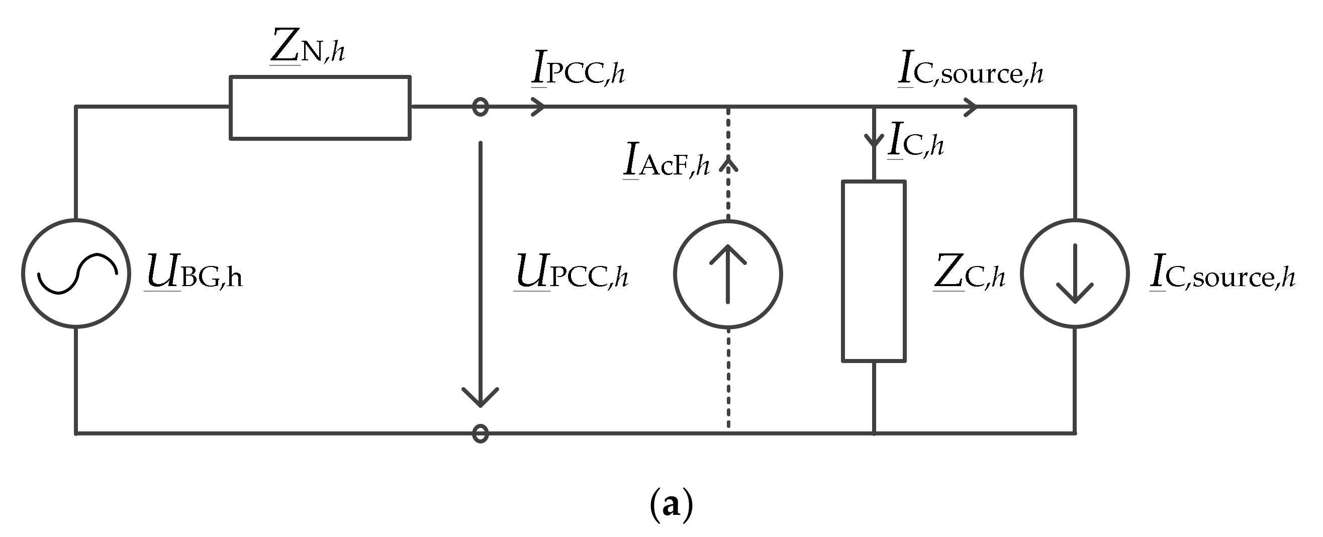
To determine the AcF reference based on the customer’s emission, the equivalent current source on the customer side and the equivalent voltage source on the network side have to be calculated. The calculation is based on the equivalent circuit given in Figure 1. The network side is represented by the Thevenin equivalent, also including other network customer emissions, because it presents background distortion at the PCC and this distortion is usually defined by harmonic voltage distortion. The customer side is represented with the Norton equivalent. For the calculation, measurements of the voltage and current harmonics (and their phase angles) at the PCC are needed, and all impedances must be known. As the actual network-side and customer-side impedances are usually not known and also change over time in a real network, reference impedances can be used instead [17,18].
Reference impedances and the determination of the customer’s emissions in the presence of active filter to the harmonic component are introduced in this section.
2.1. Customer’s Emission in Presence of the Active Filter
The proposed method for the AcF reference calculation is based on the mixed equivalent circuit shown in Figure 1, where the voltage source represents the background harmonic distortion at the harmonic component , which includes other customer emissions and background distortion (from a higher voltage level) at the PCC, given with Equation (1). The customer side is modeled with a Norton equivalent circuit. The harmonic current , which flows through the customer impedance, is caused by voltage distortion. Notably, the customer is not responsible for this harmonic current. The proposed method determines the reference for AcF, which only compensates for customer emissions—the customer harmonic current source (Equation (2)).
However, before calculating the customer harmonic emissions, the influence of the AcF on the voltage and current at the PCC must be determined. Namely, the customer emissions are calculated from the measured harmonic voltage and current, and , respectively, and clearly these quantities are influenced by the operation of the AcF, which would inevitably lead to the wrong calculation of the customer harmonic current source . To account for this influence, the apparent voltage and current quantities at the PCC are introduced with Equations (3) and (4).
As it can be seen from the equations, the apparent values of voltage () and current () are equal to the measured values of voltage and current when AcF is out of operation (i.e., ). The main influence of the AcF current is based on the main shunt device impedance (e.g., passive reactive power compensator) and network harmonic impedance (see Figure 1b). The parallel connection of shunt devices and load impedance forms the customer impedance . Because the load impedance does not have significant influence on the calculation of the apparent distortion, only the shunt device impedance is considered.
The load impedance is impossible to determine in a real environment because industrial customers typically have many loads and they change with time. The shunt device impedance is the harmonic impedance of a shunt device (e.g., passive compensator), and this impedance is only used for determining the apparent harmonic distortion. The customer emission calculation is based on the customer reference harmonic impedance (Equation (2)).
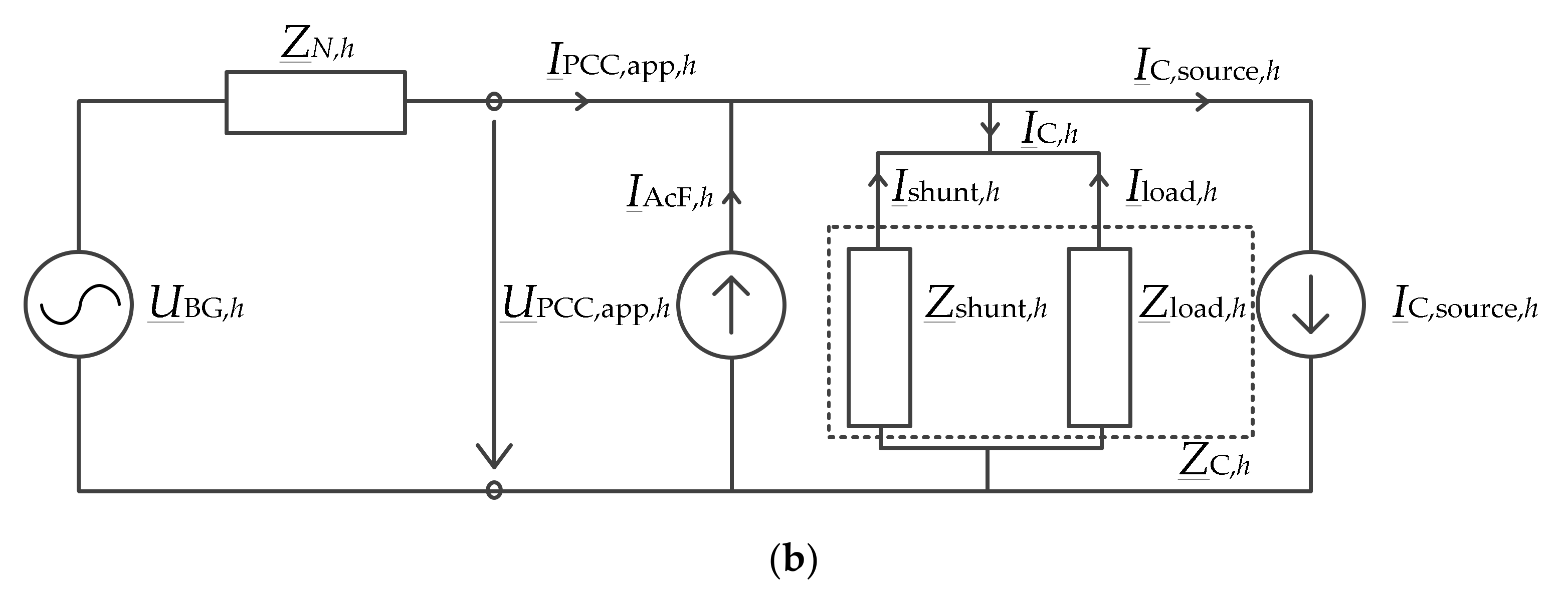
In order to maximize the AcF impact in terms of the harmonic distortion reduction at the PCC, we propose using the projection values (Equation (5)) of the current vector (customer harmonic current source) on the current vector for the AcF reference calculations. Namely, the projection value directly influences the measured current harmonic component () because it has the phase angle . An exemplary case is shown in Figure 2. Figure 2a shows the phasor diagram for the currents in Equation (2) and their projections on the vector . The projections are calculated with Equations (5) and (6). Figure 2b shows the same phasor diagram with the exception that the AcF generates the current , i.e., it compensates . The AcF reference is finally determined using Equation (7).
For the calculation of the customer’s emission in the presence of the AcF to harmonic distortion, measurements of voltage and current harmonics and their phase angles at the PCC are needed, and all impedances must be known. The reference impedances are introduced in the next section.
2.2. Reference Impedances
At the PCC, the harmonic impedances must be determined for the network and customer sides. The reference harmonic impedances on the network side of the circuit can be determined from the short-circuit ratio or from the harmonic impedance at the fundamental component. A detailed description of the calculation can be found in [17,18,19].
Customer reference impedance is defined as a resistive load (). The calculation is based on PCC measurements of the active power () and voltage () at the fundamental frequency and is given by Equation (8):
The reference customer harmonic impedance is constant for all harmonic components (). In basic terms, this means that a customer should (electrically) behave as a resistance at all harmonic frequencies, which is the same logic used for reactive power at the fundamental frequency. The difference between the customer’s actual and reference harmonic impedances translates into a change of the current source , which consequently results in a change in the customer’s emission to the harmonic distortion at the PCC.
To summarize, the customer’s emission to the harmonic current at the PCC includes not only the customer non-linear equipment but also the passive equipment causing an amplification of the harmonics due to resonances. With the customer reference harmonic impedance, the customer compensates all harmonic currents, excluding those originating from the interactions of the resistive load and the network background distortion.
3. Implementation of the Active Filter Compensation Function in the Control Algorithm
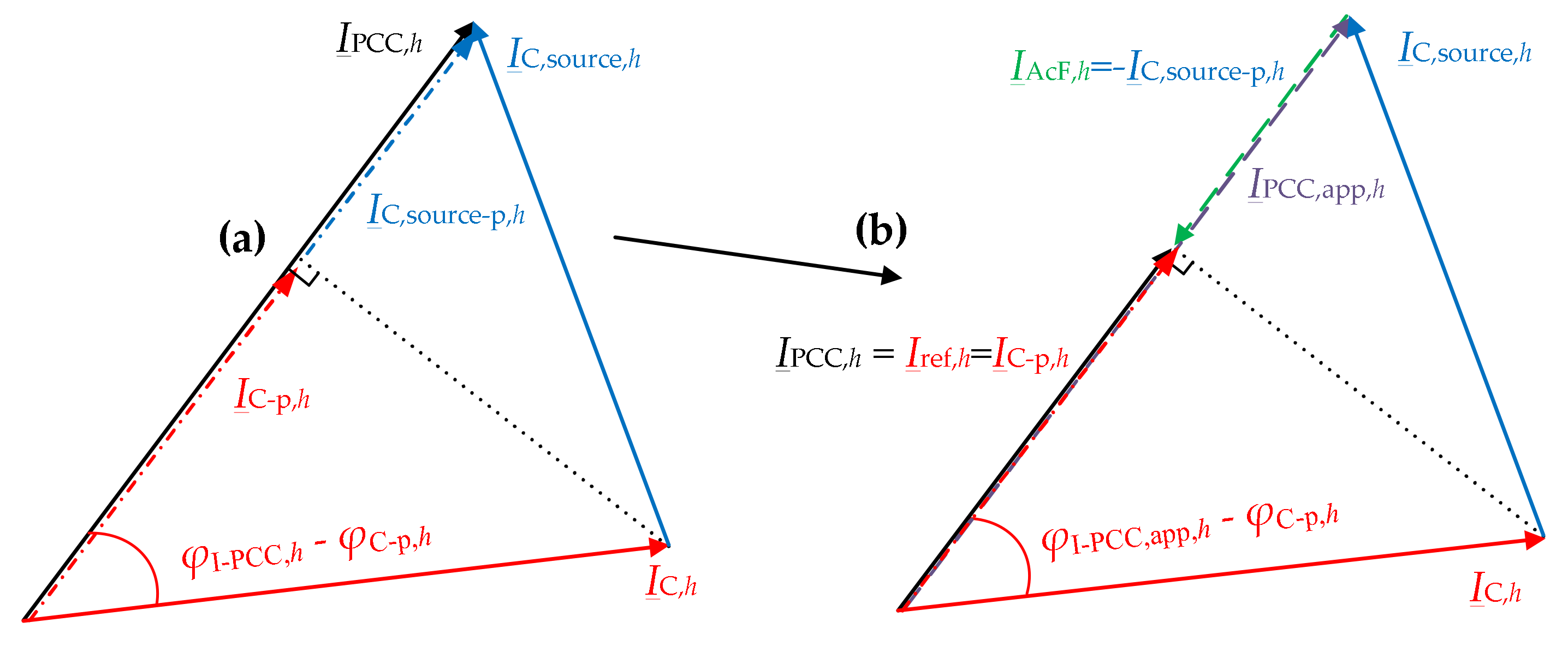
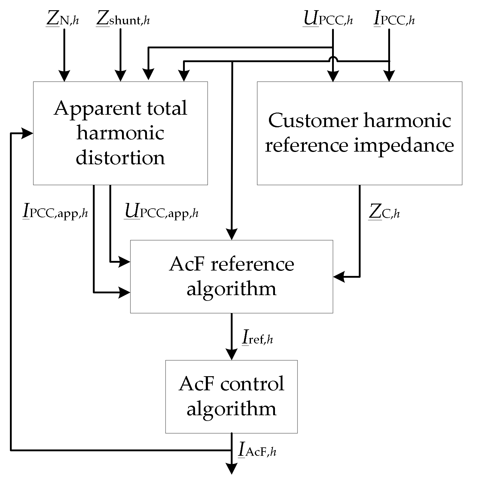
The structure of the proposed AcF compensation function based on customer emissions is given by the flowchart diagram in Figure 3. The proposed function has only four external inputs, and these inputs are the measured harmonic current and voltage , network harmonic impedance , and harmonic impedance of other customer’s shunt devices (e.g., passive reactive power compensators), which is also known or can be easily determined.
In the first block, the apparent harmonic distortion is determined, which presents the harmonic component at the PCC, when the AcF is not compensating any harmonic current. The apparent harmonic distortion is used to calculate the AcF reference in the third block, which is the main block of the compensation function. Here, the AcF reference is calculated. The inputs of the third block are the customer harmonic impedance and the apparent harmonic distortion. The AcF reference is an input to the AcF control algorithm (fourth block) that controls the filter current .
In the following subchapter, the third and fourth block are described in detail.
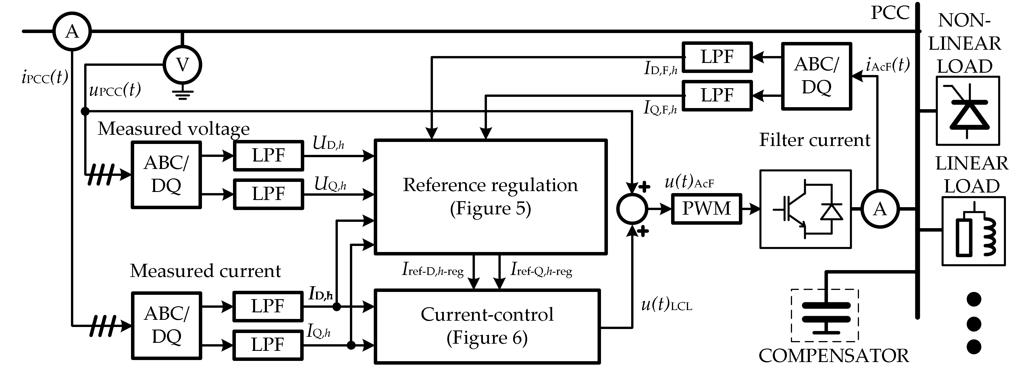
AcF Control Algorithm
To test the proposed method for the AcF reference calculations, the control block diagram shown in Figure 4, the reference control shown in Figure 5, and the current-control block diagram shown in Figure 6 were developed in PSCAD software (v4.6.0, Manitoba Hydro International Ltd., Winnipeg, MB, Canada). Each low-order harmonic component at the frequencies 250, 350, 550, and 650 Hz was extracted from the measurements at the PCC with the DQ transform using low-pass filtering (LPF), with a cut-off frequency of 10 Hz. Each harmonic component was controlled individually by the AcF.
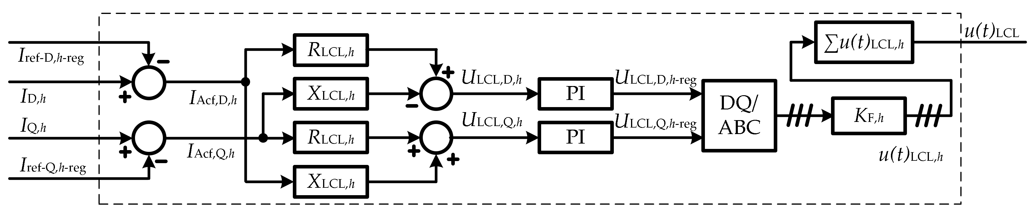
The AcF control algorithm in Figure 4 is divided into two loops: the reference calculation loop (Figure 5) and the current-control loop (Figure 6). For the current-control loops, conventional vector controllers in the DQ coordinate system were used [20,21,22] that represent an established control principle, offering a good balance between stability and performance. The switching signals for individual transistors were generated with pulse-width modulation (PWM—the switching frequency was 10 kHz). All AcF parameters are listed in Table 1.
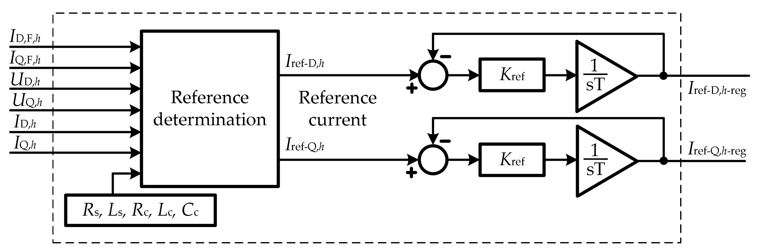
The additional control loop for AcF reference determination is provided, which includes the AcF reference algorithm and can be seen in Figure 5. The harmonic reference current (Iref-D,h and Iref-Q,h) is the output of the reference calculation block and is controlled by the gain (Kref) and integrator (Ti) to obtain the output (reference) currents of the control loop Iref-D,h-reg and Iref-Q,h-reg.
4. Simulation Results
The main aim of the simulations was to show the AcF operation with the proposed reference current calculation. The focus point was the performance of the proposed AcF reference algorithm in a network with background harmonic distortion and with impedance resonances on the customer side. Namely, these are the usual operating conditions at a distribution level. The medium-voltage benchmark model (MV BNM) [18] was used for testing the proposed method.
The results of the application of the proposed AcF reference in the MV benchmark model are presented and discussed. The analysis of the results also shows the required power ratings (reducing the filter current) of the AcF in different operating conditions. In the conventional approach, used for comparison, the AcF compensates all current harmonics at the PCC. The conventional approach is labelled as “ref. 0,” and the reference is set to zero value.
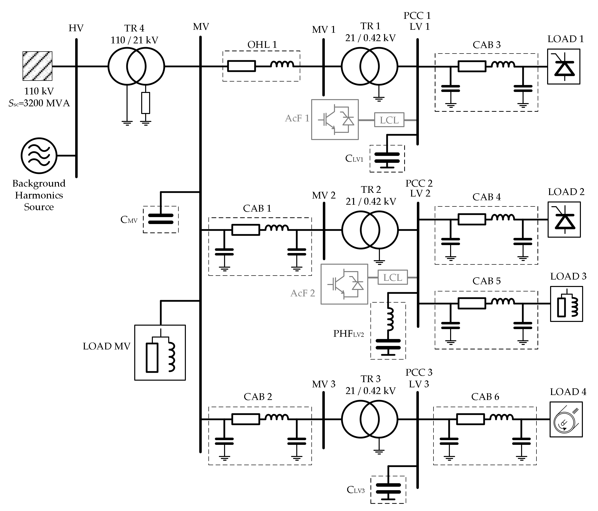
4.1. MV Benchmark Test Model Description
The proposed method was tested on the MV benchmark test model (BNM), which is shown in Figure 7 and described in detail in [18]. The MV BNM was chosen because it was developed specifically for harmonic distortion studies. This model has three customers with different equipment, including loads and passive shunt compensation. The proposed method was tested separately for Customer 1 (PCC 1) and Customer 2 (PCC 2), which is shown by the added active filters AcF 1 and AcF 2. In this paper, background harmonic distortion in the high-voltage (HV) grid was also added to the original model.
4.2. Application of the Proposed Reference Calculation Method with AcF on the MV Benchmark Model
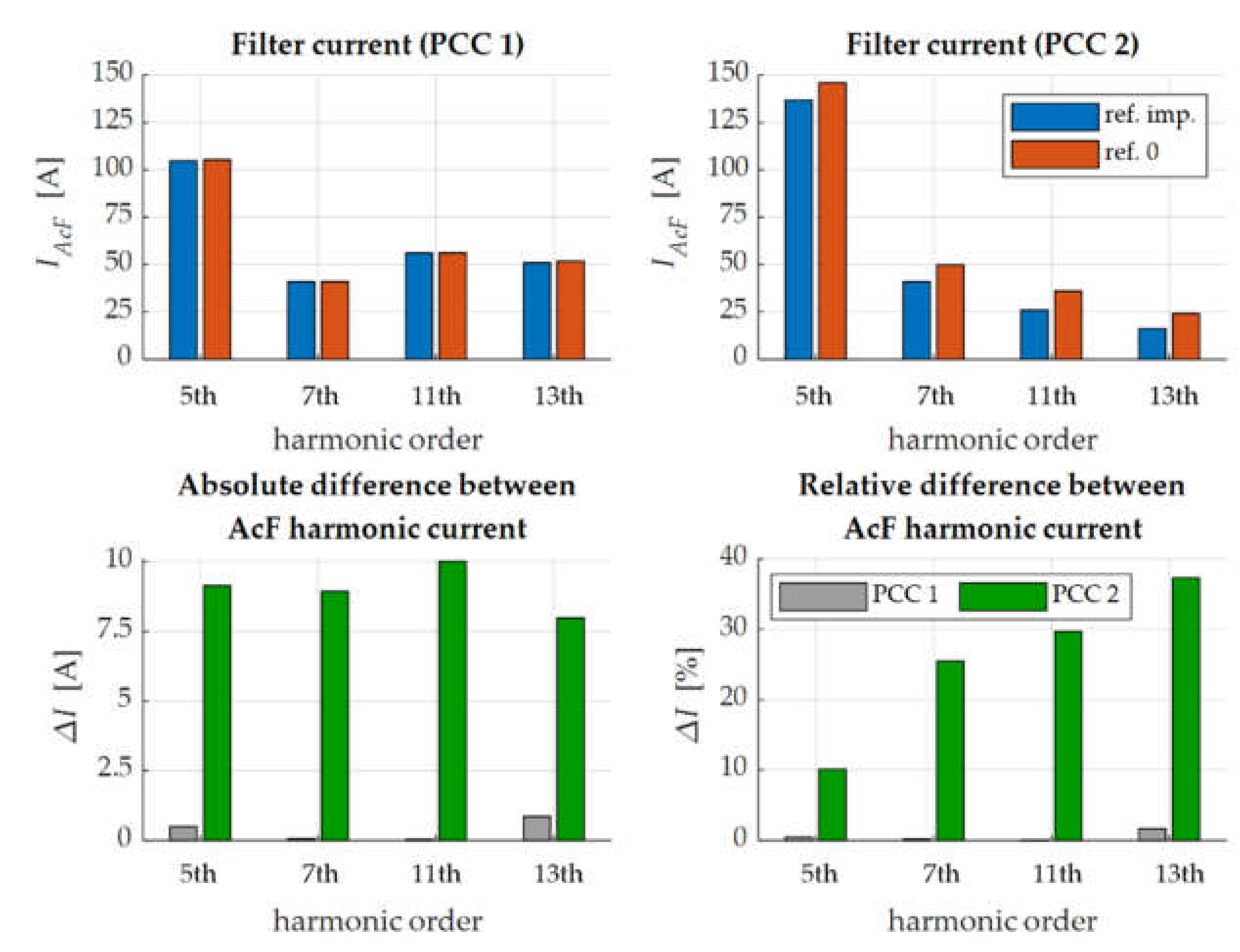
The reference calculation method of the AcF was tested on the MV benchmark model, including background distortion. The absolute value of the background distortion was constant (1.5%), whereas the phase angles changed randomly from −180° to 180° for each harmonic component. The results are shown in Figure 8, which presents the average filter current and difference between the reference impedance and conventional (compensating all harmonic current) approach. The average current is the mean value of the current at all simulated (number of simulations, ) background phase angles, as defined by Equation (9):
When the conventional case (ref. 0) was used, the AcF compensated all harmonic currents to 0. When the proposed reference was used, customers needed to compensate only the harmonic currents that deviated from the ideal resistance. Customer 1 had the resonance condition due to a detuned passive compensator (CLV1), and its impedance deviated from the ideal resistance. This is the reason why the AcF current at PCC 1 in this case was similar to the ref. 0 case (see Table 2). Customer 2 did not have any resonance conditions, which can also be seen from the customer’s results (Table 2 and Figure 8), as there is a difference between using the two approaches for calculating the AcF reference. For example, looking at the fifth harmonic component, the AcF current, calculated with the proposed reference impedance (ref. imp.), was approximately 10% lower compared to the conventional approach (ref. 0).
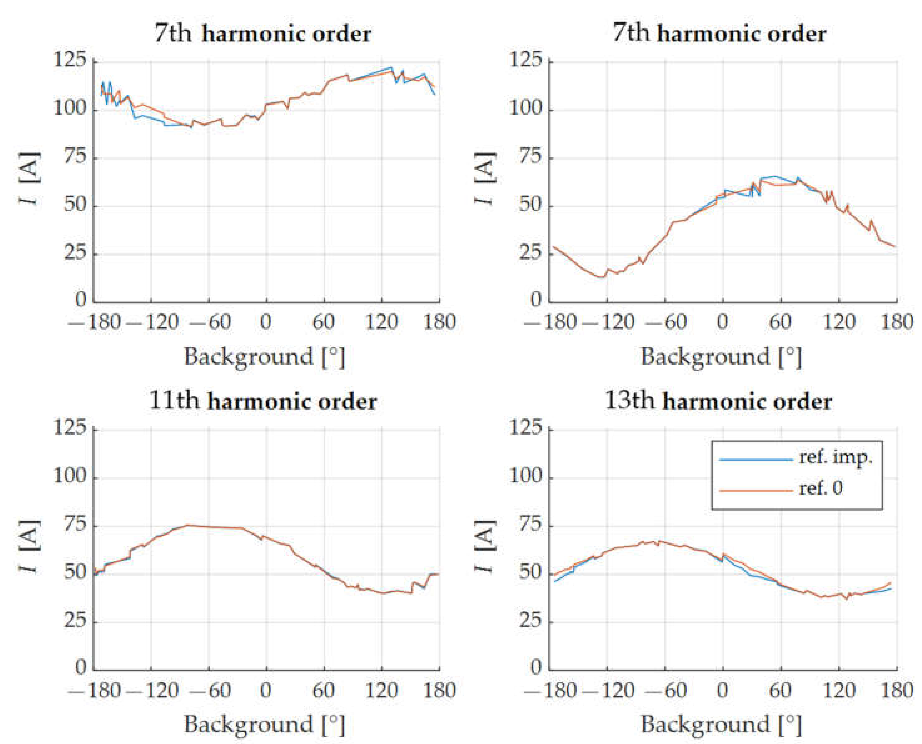
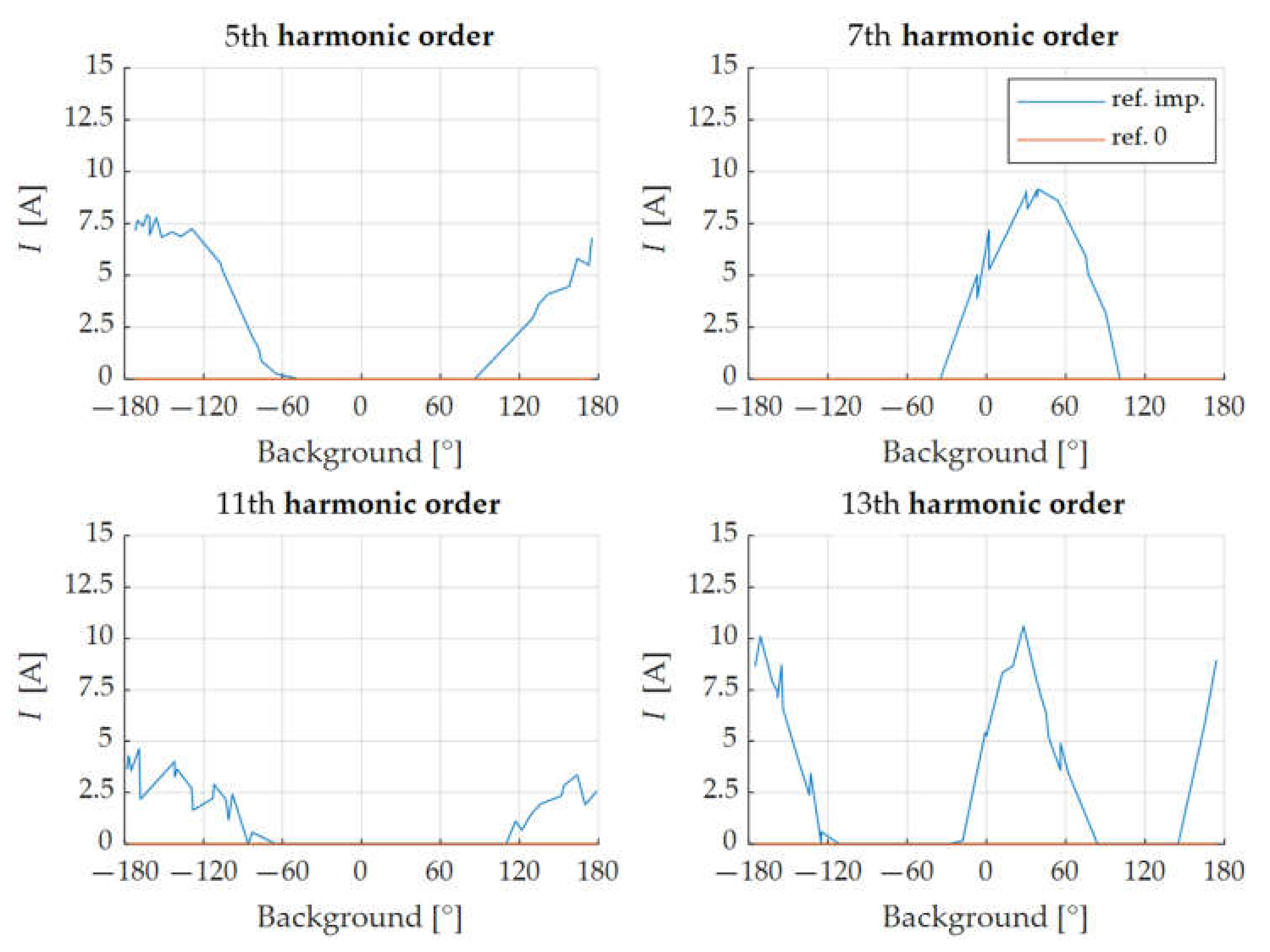
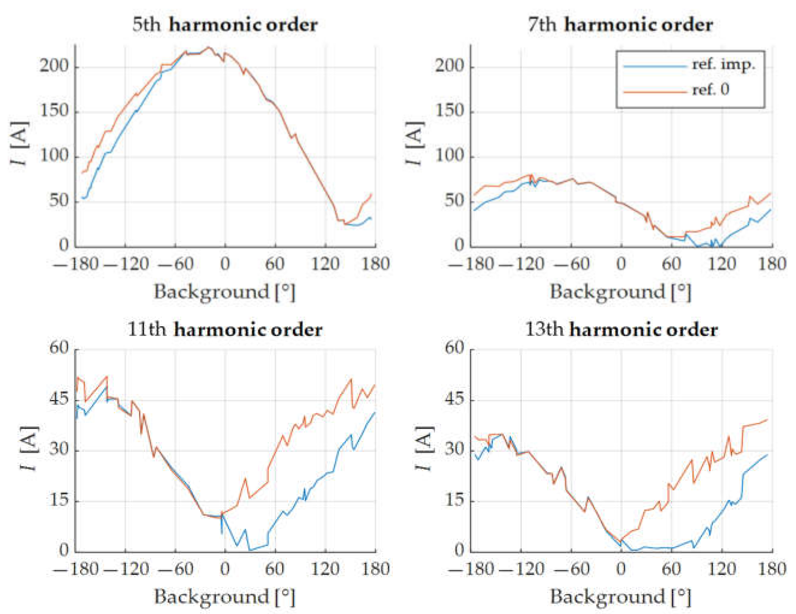
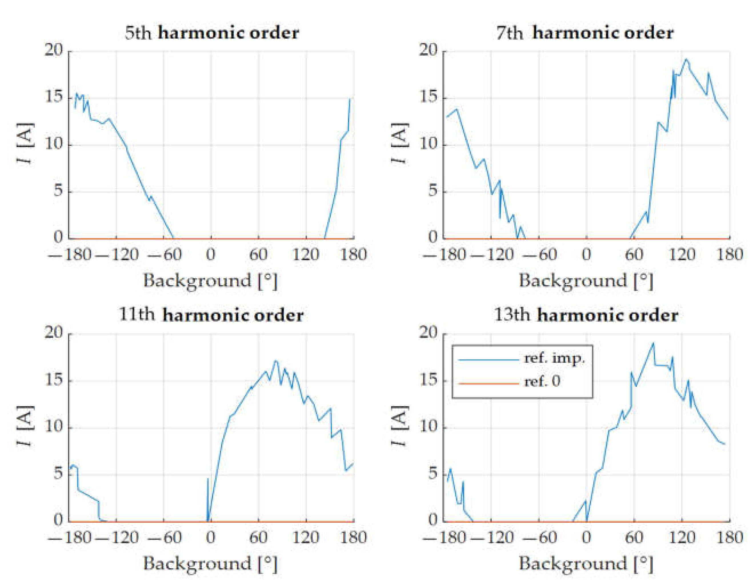
The figures below show the reference and AcF currents for different phase angles of background harmonic distortion. Figure 9 and Figure 10 show the results for PCC 1, and Figure 11 and Figure 12 show the results for PCC 2. The reference current of the AcF also provided information on how much harmonic current still flowed through the PCC after AcF compensation (see Figure 2).
The reason for the changes in the filter current with the background distortion phase angle is that with particular phase angles, the customer could compensate for or contribute to the harmonic distortion. When the customer compensated for the background distortion, the filter current decreased, and the filter current increased in the opposite case.
For Customer 1, the AcF current was comparable for both approaches. As can be seen from Figure 10, the approach of the reference impedance had a slightly lower AcF harmonic current because the AcF reference was not set to zero value at all phase angles by the reference impedance approach. The main difference in the AcF reference between approaches was at the 13th harmonic component; however, the difference was still small (see Figure 10). Customer 1 had a low impedance at the 11th harmonic impedance due to a detuned passive compensator (CLV1), and this is the reason why the difference between approaches was very low. The reference impedance approach also determined that the customer needed to compensate for all harmonic currents caused by the resonance condition.
For Customer 2, the AcF reference calculated with the reference impedances did not have zero value at all phase angles of background distortion, as can be seen in Figure 12. From Figure 12, the zero values of the AcF reference were at specific phase angles of the background distortion.
The smallest difference between the approaches as a percentage was at the fifth harmonic component, as can be observed from Figure 8, because Customer 2 had a tuned passive filter (for reactive power compensation, tuned at the fifth harmonic) that compensated for the fifth current harmonic component. This is why the AcF current was higher than at other harmonic components, as can be seen in Figure 8 and Figure 11. The difference in the AcF current (see Figure 11) and AcF reference (see Figure 12) between approaches was higher at the 7th, 11th, and 13th harmonic components because the customer harmonic impedance did not substantially deviate from the ideal resistive impedance due to the tuned passive filter (PHFLV2).
5. Conclusions
In this paper, we presented an AcF reference current calculation method based on customers’ current harmonic emissions. This method enables the consideration of only the customer’s contribution to the harmonic distortion at the PCC. The proposed method is especially beneficial when used by customers in industrial networks, where a high background harmonic distortion is often present. In such environments, the customer’s AcF does not need to compensate the harmonic current caused by the interaction of background distortion and passive loads, which reduces the required power of the AcF and, consequently, the investment and operational costs.
The theoretical analysis along with the simulation results of the proposed compensation function showed that the use of the reference harmonic impedances in the AcF controller reference calculation procedure provided good results. Using reference impedances determined, as expected, the AcF reference in accordance with the emission of the linear load, which reduced the required AcF current.
However, as the simulation results have shown, the AcF current reduction can only be achieved with customers that do not cause resonance amplification of the harmonics present in the network. In this case, when the customer’s equipment is in resonance with the network, the AcF current with the proposed compensation function is similar to the conventional approach (e.g., ref. 0). Even in such cases, using the proposed compensation function is still justified, because this ensures that future changes in the network (in particular, new linear loads) will not cause unnecessary filter loading.
As the proposed method influences only the reference calculations of the AcF controller, it can be applied to all types of AcF control algorithms. The proposed method also provides valid results when the network side or customer side changes because it is based on the reference harmonic impedance.
In the future, this research will continue with testing the AcF static and dynamic control performance on a real-time digital simulator (RTDS).
Author Contributions
Conceptualization, A.Š., I.P., and L.H.; investigation, A.Š.; methodology, A.Š., I.P., and L.H.; project administration, I.P. and L.H.; software, A.Š., B.B., and L.H.; supervision, B.B., I.P., and L.H.; validation, I.P. and L.H.; visualization, A.Š.; writing—original draft, A.Š.; writing—review and editing, A.Š., B.B., I.P. and L.H. All authors have read and agreed to the published version of the manuscript.
Funding
This research received no external funding.
Institutional Review Board Statement
Not applicable.
Informed Consent Statement
Not applicable.
Data Availability Statement
The datasets used and analyzed during the current study are available from the corresponding author on reasonable request.
Conflicts of Interest
The authors declare no conflict of interest.
References
- Akagi, H.; Watanabe, E.H.; Aredes, M. Instantaneous Power Theory and Applications to Power Conditioning, 2nd ed.; Wiley: Hoboken, NJ, USA, 2017. [Google Scholar]
- Belaidi, R.; Haddouche, A.; Guendouz, H. Fuzzy Logic Controller Based Three-Phase Shunt Active Power Filter for Compensating Harmonics and Reactive Power under Unbalanced Mains Voltages. Energy Procedia 2012, 18, 560–570. [Google Scholar]
- Hou, S.; Fei, J.; Chen, C.; Chu, Y. Finite-Time Adaptive Fuzzy-Neural-Network Control of Active Power Filter. IEEE Trans. Power Electron. 2019, 34, 10298–10313. [Google Scholar] [CrossRef]
- Devassy, S.; Singh, B. Design and Performance Analysis of Three-Phase Solar PV Integrated UPQC. IEEE Trans. Ind. Appl. 2018, 54, 73–81. [Google Scholar] [CrossRef]
- Alfaris, F.E.; Bhattacharya, S. Control and Real-Time Validation for Convertible Static Transmission Controller Enabled Dual Active Power Filters and PV Integration. IEEE Trans. Ind. Appl. 2019, 55, 4309–4320. [Google Scholar] [CrossRef]
- Devassy, S.; Singh, B. Implementation of Solar Photovoltaic System with Universal Active Filtering Capability. IEEE Trans. Ind. Appl. 2019, 55, 3926–3934. [Google Scholar] [CrossRef]
- Shukl, P.; Singh, B. Recursive Digital Filter Based Control for Power Quality Improvement of Grid Tied Solar PV System. IEEE Trans. Ind. Appl. 2020, 56, 3412–3421. [Google Scholar] [CrossRef]
- Hasan, K.N.B.Md.; Rauma, K.; Luna, A.; Candela, J.I.; Rodríguez, P. Harmonic Compensation Analysis in Offshore Wind Power Plants Using Hybrid Filters. IEEE Trans. Ind. Appl. 2014, 50, 2050–2060. [Google Scholar] [CrossRef]
- Rahmani, S.; Hamadi, A.; Al-Haddad, K.; Dessaint, L.A. A Combination of Shunt Hybrid Power Filter and Thyristor-Controlled Reactor for Power Quality. IEEE Trans. Ind. Electron. 2014, 61, 2152–2164. [Google Scholar] [CrossRef]
- Xiang, Z.; Pang, Y.; Wang, L.; Wong, C.-K.; Lam, C.-S.; Wong, M.-C. Design, control and comparative analysis of an LCLC coupling hybrid active power filter. IET Power Electron. 2020, 13, 1207–1217. [Google Scholar] [CrossRef]
- Chen, X.; Dai, K.; Xu, C.; Peng, L.; Zhang, Y. Harmonic compensation and resonance damping for SAPF with selective closed-loop regulation of terminal voltage. IET Power Electron. 2017, 10, 619–629. [Google Scholar] [CrossRef]
- Yi, H.; Zhuo, F.; Zhang, Y.; Li, Y.; Zhan, W.; Chen, W.; Liu, J. A Source-Current-Detected Shunt Active Power Filter Control Scheme Based on Vector Resonant Controller. IEEE Trans. Ind. Appl. 2014, 50, 1953–1965. [Google Scholar] [CrossRef]
- Biswas, P.P.; Suganthan, P.N.; Amaratunga, G.A.J. Minimizing harmonic distortion in power system with optimal design of hybrid active power filter using differential evolution. Appl. Soft Comput. 2017, 61, 486–496. [Google Scholar] [CrossRef]
- Electromagnetic Compatibility (EMC)-Part 3-6 Limits-Assessment of Emission Limits for the Connection of Distorting Installations to MV, HV and EHV Power Systems; IEC TR Std. 61000-3-6; International Electrotechnical Commission: Geneva, Switzerland, 2008.
- Voltage Charecteristic of Electricity Supplied by Public Electricity Networks; EN 50160:2010; CENELEC: Brussels, Belgium, 2010.
- IEEE Recommended Practice and Requirements for Harmonic Constrol in Electric Power Systems; IEEE 519-2014; IEEE: New York, NY, USA, 2014.
- Pfajfar, T.; Blazic, B.; Papic, I. Harmonic Contributions Evaluation with the Harmonic Current Vector Method. IEEE Trans. Power Deliv. 2008, 23, 425–433. [Google Scholar] [CrossRef]
- Papič, I.; Matvoz, D.; Špelko, A.; Xu, W.; Wang, Y.; Mueller, D.; Miller, C.; Ribeiro, P.F.; Langella, R.; Testa, A. A Benchmark Test System to Evaluate Methods of Harmonic Contribution Determination. IEEE Trans. Power Deliv. 2019, 34, 23–31. [Google Scholar] [CrossRef]
- Špelko, A.; Blažič, B.; Papič, I.; Pourarab, M.; Meyer, J.; Xu, X.; Djokic, S.Z. CIGRE/CIRED JWG C4.42: Overview of common methods for assessment of harmonic contribution from customer installation. In Proceedings of the 2017 IEEE Manchester PowerTech, Manchester, UK, 18–22 June 2017; pp. 1–6. [Google Scholar]
- Božiček, A.; Papič, I.; Blažič, B. Performance evaluation of the DSP-based improved time-optimal current controller for STATCOM. Int. J. Electr. Power Energy Syst. 2017, 91, 209–221. [Google Scholar] [CrossRef]
- Herman, L.; Božiček, A.; Blažič, B.; Papič, I. Real-time simulations of a parallel hybrid active filter with hardware-in-the-loop. In Proceedings of the 2014 16th International Conference on Harmonics and Quality of Power (ICHQP), Bucharest, Romania, 25–28 May 2014; pp. 576–580. [Google Scholar]
- Božiček, A.; Blažič, B.; Papič, I. Time-optimal operation of a predictive current controller for voltage source converters. In Proceedings of the 2011 International Conference on Power Engineering, Energy and Electrical Drives, Malaga, Spain, 11–13 May 2011; pp. 1–7. [Google Scholar]
Figure 1.
Mixed equivalent circuit at harmonic component h: (a) general representation and (b) configuration for calculation of the apparent values of point of common coupling (PCC) harmonic voltage and current.
Figure 1.
Mixed equivalent circuit at harmonic component h: (a) general representation and (b) configuration for calculation of the apparent values of point of common coupling (PCC) harmonic voltage and current.


Figure 2.
Phasor diagram of customers’ currents (a) without active filter (AcF) and (b) with AcF.

Figure 3.
Flow chart diagram.

Figure 4.
Control block diagram of the AcF.

Figure 5.
Reference regulation block diagram.

Figure 6.
Current-control block diagram.

Figure 7.
The medium-voltage (MV) benchmark model [18].
Figure 7.
The medium-voltage (MV) benchmark model [18].

Figure 8.
Comparison of the average AcF harmonic currents and the difference.

Figure 9.
Filter current at PCC 1.

Figure 10.
Reference current at PCC 1.

Figure 11.
Filter current at PCC 2.

Figure 12.
Reference current at PCC 2.


Table 1.
The control parameters.
| KF,h | Regulator Parameters | LCL Filter | ||
|---|---|---|---|---|
| Harmonic Order | PCC1 | PCC2 | PCC1 and PCC2 | LLCL,1 = 0.1 mH |
| 5th | −1 | −1 | Kref = 0.5 | LLCL,2 = 0.01 mH |
| 7th | 1 | 1 | Ti = 0.01 | RLCL,1 = RLCL,2 = 0.001 Ω |
| 11th | 1 | −1 | Kp = 1 | RLCL = 0.001 Ω |
| 13th | −1 | 1 | CLCL = 42 μF | |
Table 2.
Results showing the average AcF harmonic currents.
| PCC 1 | PCC 2 | |||||||
|---|---|---|---|---|---|---|---|---|
| Harmonic Order | Ref. 0 [A] | Ref. Imp. [A] | Difference [A] | Difference [%] | Ref. 0 [A] | Ref. Imp. [A] | Difference [A] | Difference [%] |
| 5th | 105.26 | 104.77 | 0.49 | 0.47 | 145.93 | 136.79 | 9.14 | 10.11 |
| 7th | 40.97 | 40.91 | 0.06 | 0.18 | 49.82 | 40.89 | 8.93 | 25.49 |
| 11th | 56.13 | 56.09 | 0.04 | 0.08 | 35.97 | 25.96 | 10.01 | 29.70 |
| 13th | 51.78 | 50.93 | 0.86 | 1.66 | 24.10 | 16.12 | 7.98 | 37.28 |
Publisher’s Note: MDPI stays neutral with regard to jurisdictional claims in published maps and institutional affiliations. |
© 2021 by the authors. Licensee MDPI, Basel, Switzerland. This article is an open access article distributed under the terms and conditions of the Creative Commons Attribution (CC BY) license (http://creativecommons.org/licenses/by/4.0/).
Share and Cite
MDPI and ACS Style
Špelko, A.; Blažič, B.; Papič, I.; Herman, L. Active Filter Reference Calculations Based on Customers’ Current Harmonic Emissions. Energies 2021, 14, 220. https://doi.org/10.3390/en14010220
AMA Style
Špelko A, Blažič B, Papič I, Herman L. Active Filter Reference Calculations Based on Customers’ Current Harmonic Emissions. Energies. 2021; 14(1):220. https://doi.org/10.3390/en14010220
Chicago/Turabian StyleŠpelko, Aljaž, Boštjan Blažič, Igor Papič, and Leopold Herman. 2021. "Active Filter Reference Calculations Based on Customers’ Current Harmonic Emissions" Energies 14, no. 1: 220. https://doi.org/10.3390/en14010220
Note that from the first issue of 2016, this journal uses article numbers instead of page numbers. See further details here.