Software Solution for Modeling, Sizing, and Allocation of Active Power Filters in Distribution Networks


Electrical Engineering and Computer Science Department, Faculty of Electrical Engineering, Silesian University of Technology, 44-100 Gliwice, Poland
*
Author to whom correspondence should be addressed.
Energies 2021, 14(1), 133; https://doi.org/10.3390/en14010133
Submission received: 23 November 2020
/
Revised: 14 December 2020
/
Accepted: 23 December 2020
/
Published: 29 December 2020
(This article belongs to the Special Issue Active Power Filters and Power Quality)
Abstract
:The paper is related to the problem of modeling and optimizing power systems supplying, among others, nonlinear loads. A software solution that allows the modeling and simulation of power systems in the frequency domain as well as the sizing and allocation of active power filters has been developed and presented. The basic assumptions for the software development followed by the models of power system components and the optimization assumptions have been described in the paper. On the basis of an example of a low-voltage network, an analysis of the selection of the number and allocation of active power filters was carried out in terms of minimizing losses and investment costs under the assumed conditions for voltage total harmonic distortion (THD) coefficients in the network nodes. The presented examples show that the appropriate software allows for an in-depth analysis of possible solutions and, furthermore, the selection of the optimal one for a specific case, depending on the adopted limitations, expected effects, and investment costs. In addition, a very high computational efficiency of the adopted approach to modeling and simulation has been demonstrated, despite the use of (i) element models for which parameters depend on the operating point (named iterative elements), (ii) active filter models taking into account real harmonics reduction efficiency and power losses, and (iii) a brute force algorithm for optimization.
1. Introduction
This paper is the result of a few years of research related to the active power filter sizing and allocation in a power supply system with distorted current and voltage waveforms. Studies have shown that this issue has a significant impact both on the quality of compensation and the cost of active power filter (APF) connection. The algorithms developed to optimize the sizing and placement of active power filters [1] and hybrid active power filters [2] brought the expected results [3,4,5]. In particular, they allowed analyzing the possibility of minimizing the investment cost in the case of using active compensation. At the time when the authors started their first research work (2010), the issue of APF placement optimization had not yet been widely analyzed in international publications [6,7,8]. Currently, with the increase in the use of active compensation, many scientists are conducting research on the optimization placement of passive [9] and active [10] compensators. The possibilities of using various optimization approaches and algorithms are analyzed, i.e., particle swarm optimization (PSO) [11], music-inspired [12], firefly [13], grey wolf [14], differential evolution algorithm (DEA) [15], genetic algorithm (GA) [16,17], fuzzy [18,19,20], trade-off/risk [21] and others aimed at assessing the possibility of minimizing the power losses [22,23]. New research works are also related to the use of the optimal allocation of power quality conditioners in microgrid networks [24,25,26], which is related to the increasing content of this type of installations in the global power network.
The analysis of the power supply system using a numerical simulation requires two basic components: component models and software for the analysis of the system state. This software can additionally implement the system’s working point optimization (according to a given criterion). A model can be defined as a set of assumptions, concepts, and relationships between them, allowing describing (usually in an approximate way) a certain selected fragment of reality. Most often, the language of mathematics is used to describe the model. The complexity of the power system requires the use of various types of simplifications, both in the area of model parameters identification and in the area of analysis. The most important thing is to ignore all nonlinearities that may occur in the system. Computer methods of system analysis most often use the so-called frequency method [27], which uses the decomposition of current and voltage waveforms in the Fourier series (additionally, other types of modeling, such as hybrid [28] or fractional order [29], are also developed). For each of the components of the Fourier series obtained in this way, the relationships between the current and voltage as well as the impedances of individual system components for the considered harmonics are determined. In this way, the amplitude-frequency and phase-frequency characteristics of the system are obtained. This type of analysis is possible with the assumption that the analysed signals are periodic. This is the most commonly used method for quasi-steady state system analysis. The software used so far for this type of analysis can be divided into two basic groups:
- Dedicated to harmonic analysis, including commercial software, such as ETAP or research and educational software, such as PCFLO,
- General-purpose software, such as numerical computing environments such as Mathematica or Matlab.
The use of software from the second group allows us to not only to analyze the system but also to perform additional tasks, e.g., optimization of the sizing and placement of active power filters in the system, as it is associated with a large number of built-in libraries. However, this requires the development and verification of a basic module that calculates the power flow for individual harmonics. In this case, a good solution seems to be the combination of the properties of programs from both groups. Table 1 and Table 2 show a comparison of the functionality and capabilities of the available software dedicated to the power system analysis. The harmonic analysis (HA) column presents the possibility of analyzing systems containing higher harmonics in the supply current and voltage waveforms [30].
The analysis of the properties of the available software showed that there is no comprehensive solution on the market that would allow not only power flow optimization but also a definable criterion for optimizing the sizing and placement of active filters for compensating the negative impact of nonlinear receivers. As part of the previous research, hybrid software was developed, which was a combination of a program calculating the power flow and implementing harmonic analysis (PCFLO) and a general-purpose mathematical package (MATLAB), which implemented optimization solutions. This concept allowed us to obtain effective solutions but also showed very large limitations and a high demand for computing power. For example, Table 3 shows the calculation time of the optimal placement of 2 to 16 APF/HAPF in 16 nodes of a 445-node power supply system [31].
The results of the experiments obtained by the authors at this stage were used to develop new software that would enable not only the analysis of the steady state of the power supply system (in the frequency domain) but also the optimization of active power filter sizing and placement to obtain the operating state of the power supply system according to a given criterion [32]. The authors’ original contribution is the development of a fast and flexible modeling and simulation library with a new algorithm based on the frequency domain method and linear algebra. This algorithm allows the inclusion of nonlinear elements in simulations, such as constant power loads or APFs, as described later in this article. Furthermore, the flexibility of the proposed solution makes the use of additional elements dependent on higher harmonics in the models possible. An example is the proposed transformer model, taking into account power losses from eddy currents for higher harmonics. The computational efficiency of this solution allows application of the proposed approach to modeling and simulation in case of optimization problems of the power supply system in a steady state. According to the authors, this solution is unique on a global scale and may contribute to the popularization of the use of active power filters as the best solution to eliminate higher harmonics from current and voltage waveforms, which, due to high investment costs, is often replaced with a passive compensation. A further part of the paper describes the developed modeling and simulation algorithm, a description of exemplary models of the power system elements, and the results of the analysis of a real power system in one of the coal mines in Poland.
2. Pqs-Core—Frequency Domain Software Modeling Framework for Power System Simulation
In order to perform a computer simulation of a power system containing active power filters, a Java programming language library named “pqs-core” was developed. The library allows modeling power systems in the frequency domain. Earlier work has shown [33] that the frequency model can be sufficiently accurate from a power flow and harmonic flow point of view while maintaining a high computational efficiency. The computational efficiency is particularly important when iterative algorithms such as optimization, stochastic analysis, etc., are considered. The main features of the developed library are:
- Application of frequency models is based on the Fourier series (the current injection model in particular [34]).
- The main simulation algorithm is based on the Modified Nodal Analysis [35] extended for the harmonic model.
- The possibility to model any nonlinear and iterative element with a known frequency model (the iterative model’s operating point is found during the simulation).
- The ability to recursively define subsystems of any degree of complexity (each system can contain any number of nested subsystems).
- The possibility to integrate any algorithm in the higher layers of the library (e.g., optimization algorithms, stochastic analysis, etc.).
- No practical restrictions on the size of the system (the practical size depends on the available memory and computing power).
- Fully native Java code allows portability between different platforms and easy integration with other libraries (GUI, databases, etc.) and computing packages (e.g., Matlab).
- A simple and effective way of defining systems/subsystems ensuring code transparency.
- Full access to the source code and no restrictions on third party copyrights.
Development of the pqs-core library was deemed necessary, as none of the analysed computational packages provided all of the above-mentioned features simultaneously.
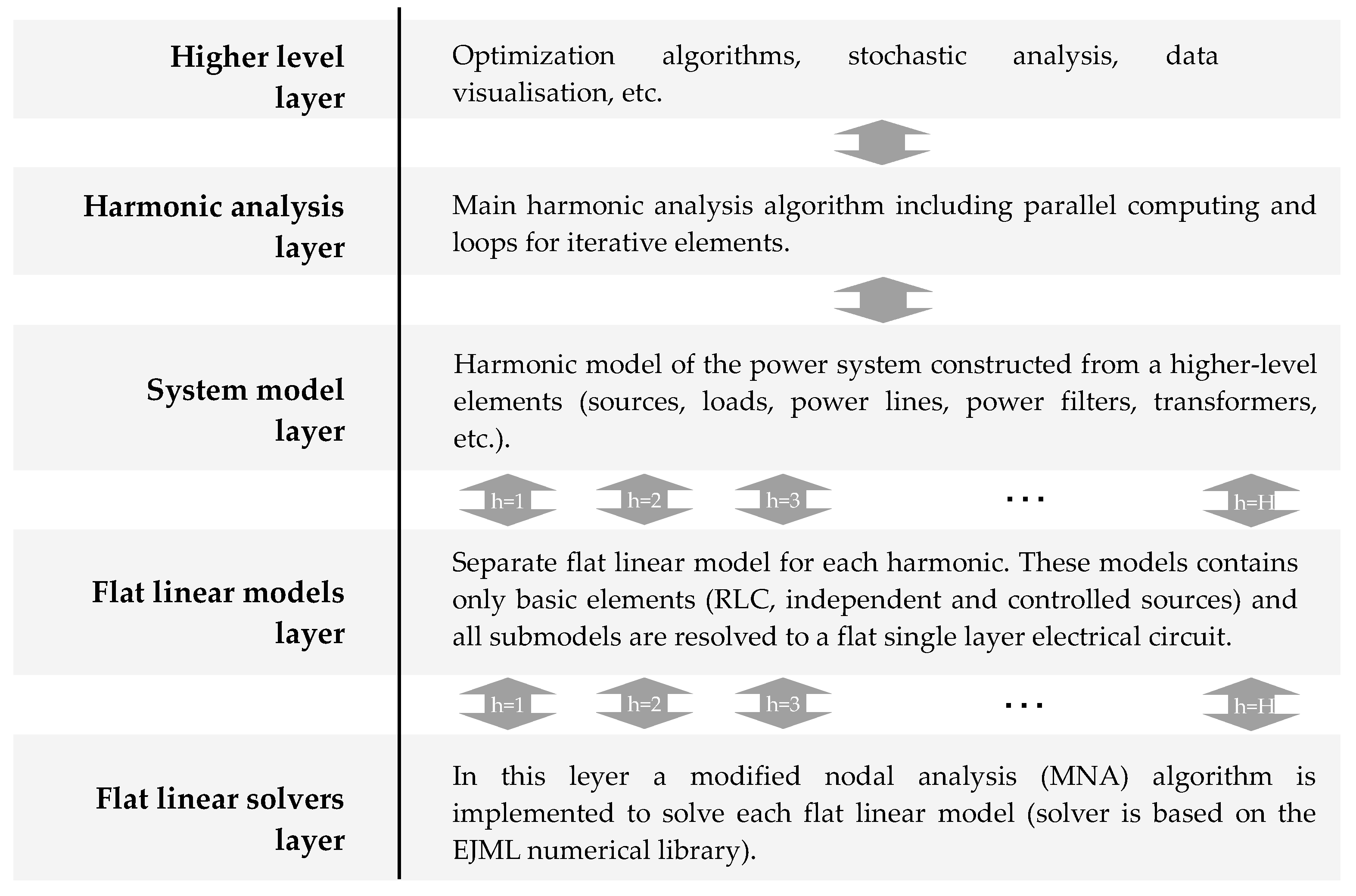
A general model of the developed pqs-core library is shown in Figure 1.
The higher-level layer of the pqs-core library (Figure 1) allows for the implementation of algorithms that are controlling the harmonic analysis layer (e.g., optimization algorithms) as well as providing tools for visualization of the obtained simulation results.
The harmonic analysis layer contains the main algorithm that computes the Fourier spectra of all currents and voltages in the power system for a selected harmonic range [1, H]. The implemented simulation algorithm is multithreaded and allows for the parallel computing of higher-order harmonics.
The system model layer allows the definition of an element connection list (topology) of the considered power system. Then, the defined model is reduced to the so-called “flat linear models”, which are independent for each single harmonic. This approach allows the defined models to be amorphous, i.e., for each harmonic, the model may contain other types of basic components (e.g., impedance for the first harmonic and current source for the higher harmonics). Flat linear models are single-layer models (all subsystems are unraveled) and contain only the basic R, L, C elements and autonomous and controlled current and voltage sources. From a circuit theory point of view, flat linear models are SLS class circuits generated separately for each harmonic at a certain operating point of the system.
In the lowest layer of the library, there is a separate solver object for each flat linear model. The solvers are based on the frequently used modified nodal analysis (MNA) and use the EJML library for calculations on complex matrices. The EJML library was selected because in the performed tests, it turned out to be the fastest among other Java numerical libraries. A computing speed comparison of selected libraries/computing packages is presented in Table 4. The initial selection of libraries was made upon publicly available tests [36].
The summary presented in Table 4 clearly shows that the best performance among Java libraries was achieved by the EJML library. There is also a clear discrepancy between the different libraries, especially when a large number of variables are considered. For example, the Apache Commons Math library for 1600 variables is over twenty times slower than EJML, although with 50 variables, the difference is only a few dozen percent. It can also be seen that the native solutions (Fortran/C++) used in Matlab and Scilab still guarantee the best computing performance. It is also worth mentioning that the pqs-core library enables (if necessary) the use of an external solver written in C++.
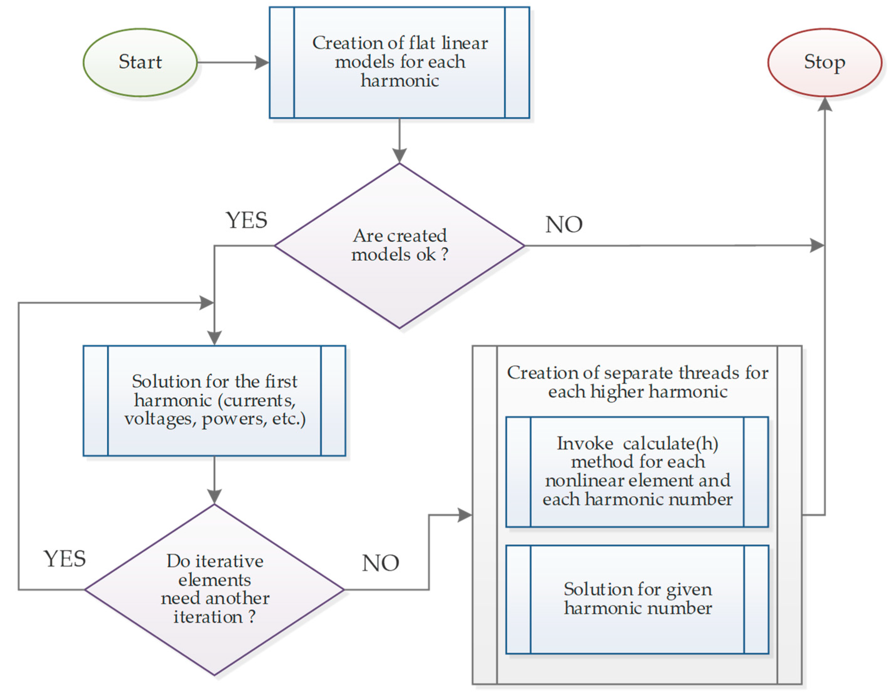
Figure 2 shows the main harmonic analysis algorithm. The algorithm allows us to perform simulations for a system containing linear, nonlinear, and iterative elements. The calculations are carried out at a certain operating point of the system and for each harmonic component. Therefore, the general assumptions for this algorithm are similar to the simulation methods used in popular programs (e.g., AC analysis in PSpice).
In the first step, the algorithm creates a flat linear model for each harmonic component. If the created models are considered correct, the model for the first harmonic is solved. This process can be iterative if the model contains elements described by parameters that are operating point dependant (e.g., loads with constant power consumption). The iterative process is performed using the fixed point method [37], which turned out to be entirely sufficient in this case. Since the operating point of the system is practically always close to the starting point of the algorithm (usually the nominal parameters of the system), even such a simple algorithm ensures good numerical stability and the achievement of the assumed accuracy in just a few iterations. After reaching the solution for the first harmonic, the operating point of the circuit is known, and thus the parameters of the nonlinear models for higher harmonics can be completely determined (it is assumed that a relationship between the first harmonic and the higher harmonics of the model may exist).
In the next step, the flat models for higher harmonics can be solved. Due to the fact that the flat models are fully independent of each other, calculations can be carried out in parallel, which in typical situations leads to a several times faster simulation (in the tested cases, the results were achieved about five times faster using four cores and eight threads). After completing the simulation process for all harmonics, the results are fed back to the system model for further analysis/visualization.
3. Harmonic Models of Power System Elements
3.1. Active Power Filters
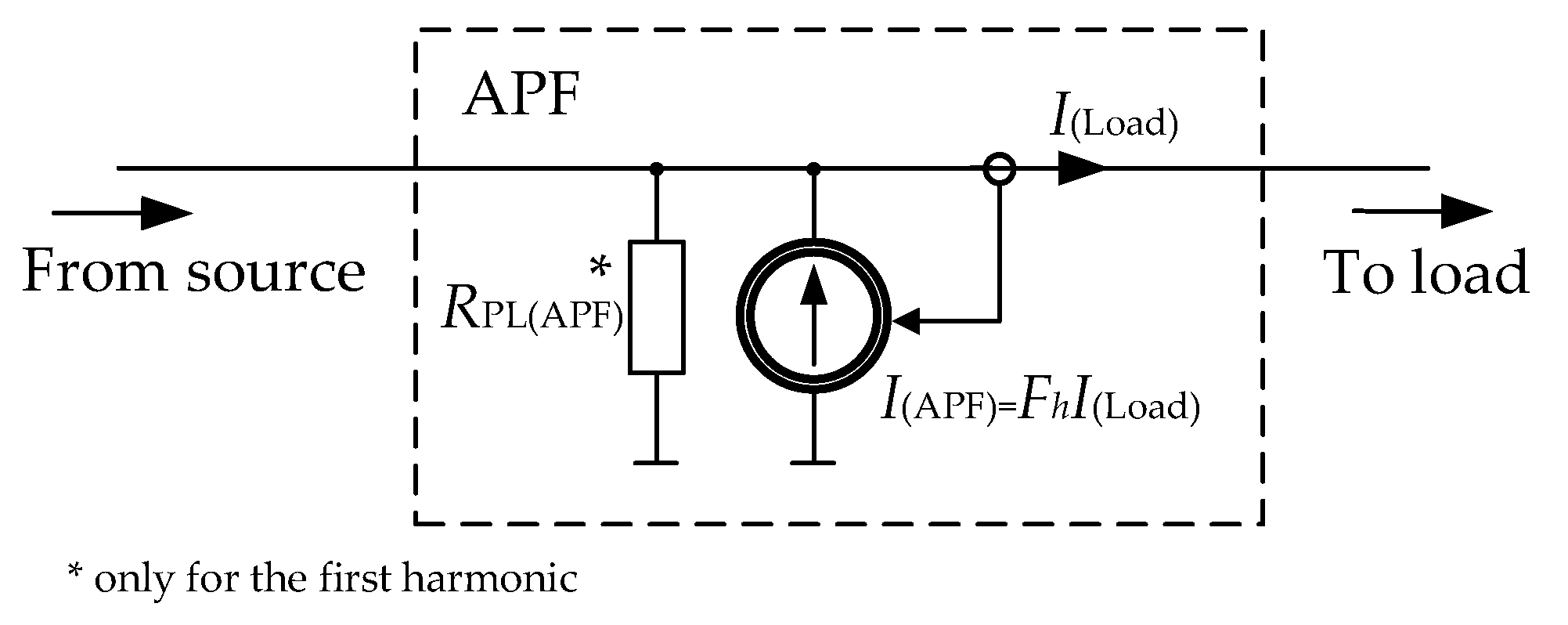
In the presented software, the active power filters have been modeled as current sources controlled by the load current. It was assumed that the active filter reduces the reactive power for the first harmonic and the higher harmonics of the load current. The model is shown in Figure 3.
This approach allows the determination of the control coefficients Fh independently for each harmonic. For the first harmonic, the control coefficient depends on reactive power. The reactive power of the fundamental harmonic should have the same value and opposite sign as the reactive power of load:
Meanwhile, the active power should be zero, so that:
Taking the above into consideration, one can write:
Thus,
Finally, the gain coefficient of the current source (APF) for the first harmonic is:
As one can notice, this coefficient depends on the load current, whereas it depends on the voltage operating point so that for the first harmonic, the APF model is an iterative element.
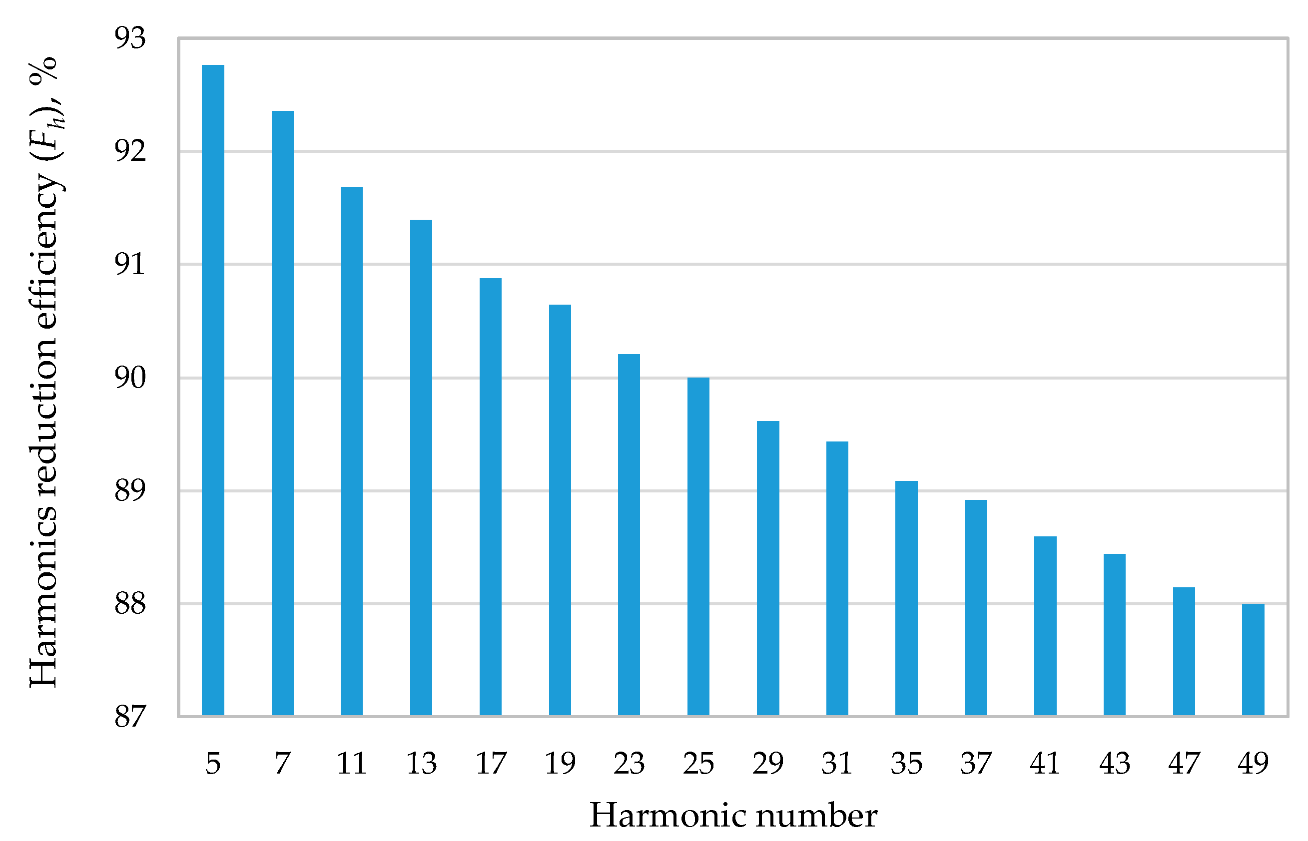
In the ideal case, for higher harmonics, the value of the control factor Fh is equal to one. However, in this case, it has been assumed that the efficiency of higher harmonic reduction is not ideal and depends on the harmonic number according to the characteristics in Figure 4.
Moreover, the implemented model of an active filter assumes that its power efficiency is defined as:
While takes a value of 98%. The active power losses have been modeled as additional resistors for the first harmonic in a parallel connection with APF. The value of the resistors depends on the APF apparent power and the first harmonic voltage value in operation point (9).
3.2. Loads
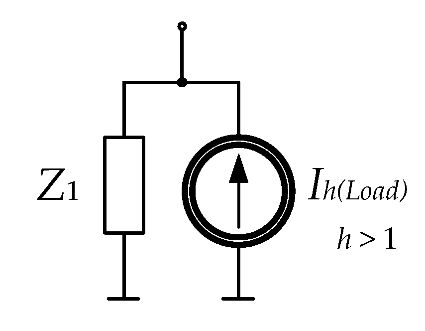
The nonlinear loads have been modeled as a linear impendence for the first harmonic and a current source for the higher harmonics (Figure 5). The impendence value depends on the requested active power and the power factor cos(φ) for the fundamental harmonic.
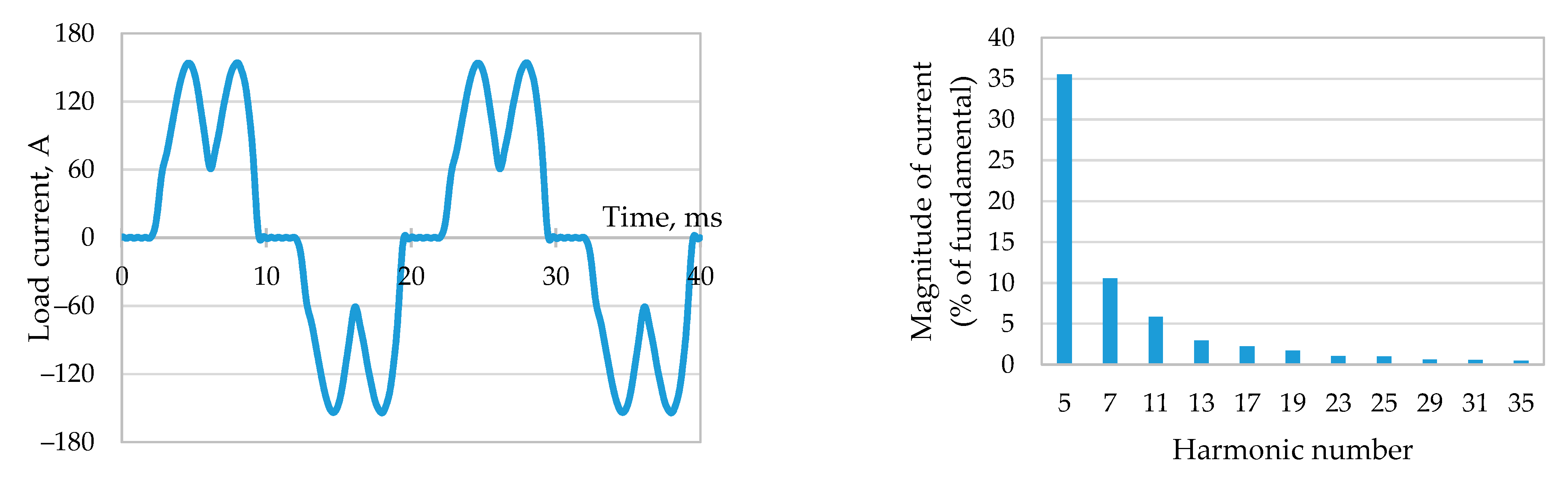
In the following example, the characteristics of a typical electric drive powered by an inverter (Figure 6) have been used. Due to the constant active power of the load, the impedance value for the first harmonic depends on the supply voltage. Therefore, for the first harmonic, it is an iterative element in the simulations.
3.3. Transformers and Lines
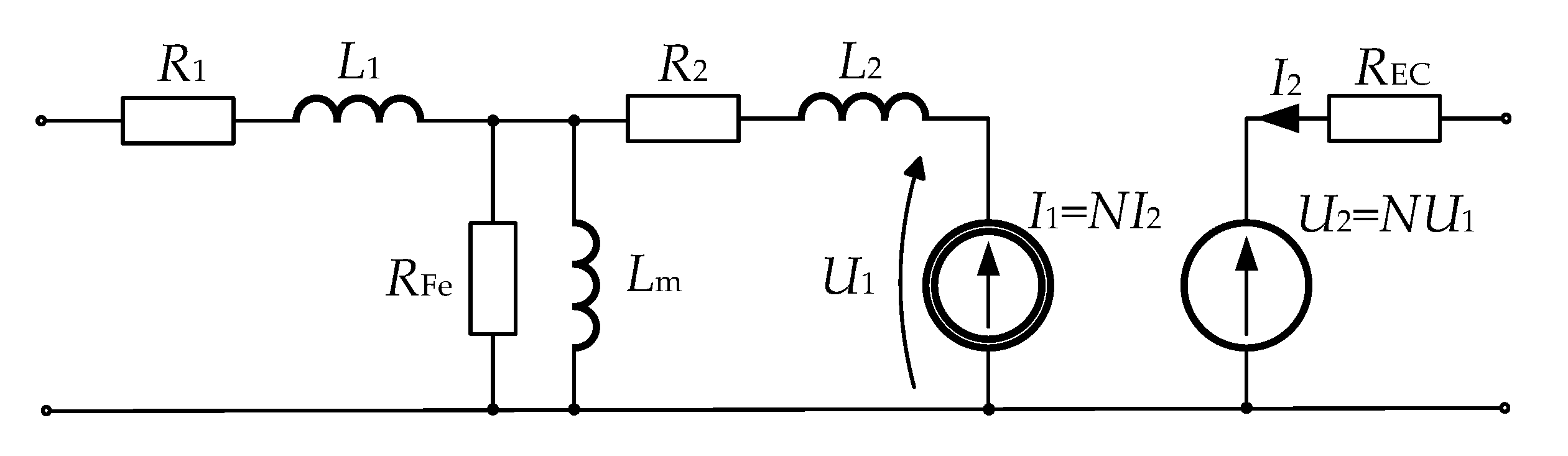
The model of the single-phase transformer shown in Figure 7 has been implemented in the presented software.
Most of the transformer model elements have been written about and reviewed in other papers and works [38], and their parameter values directly result from the data sheets of the transformers. However, an additional element is the resistor REC, which represents the influence of the eddy current losses. According to [39,40,41], the value of the eddy current losses depends on the square of the current harmonic number, i.e.,:
where
- PEC-R represents the winding eddy current losses for the sinusoidal rated load,
- PEC represents the corresponding losses for the non-sinusoidal load, and IR is the rated current.
Based on (10), one can obtain the active power for each h-harmonic:
The current Ih flowing thorough the resistor REC is known, so one can write:
Equation (12) shows the dependence of the resistance on the nominal parameters of the transformer and the square value of the harmonic number. The eddy current losses for the first harmonic differ depending on the transformer construction, and it can take a value from 1% to 20% of the total load losses [41]. In the analyzed example, losses equal to 10% have been assumed.
4. Power Loses and APF Cost Minimization
It is increasingly popular to apply an optimization approach for the sizing and allocation of active power filters [3,10,42,43]. The high cost of APFs makes optimization an essential step toward their wider application. The literature overview reveals that the research undertaken in this field takes into account the minimization of the filter RMS currents or the THD coefficients in the network and often does not include the economic criteria [44,45,46]. The distinctive feature of this paper consists not only in applying an economic approach but also in the minimization of the power losses caused by the higher harmonics in all system elements (mainly electric cables and transformers). Such a methodology is especially useful in relatively small networks working with almost no power margin and thus vulnerable to overloads or replacement of key and expensive components such as transformers. This paper follows the recommendation pointed out in [4] and is based on the conclusion that the optimization of APF sizes and allocation should one way or another include the economic consequences of the solution.
This paper is a continuation of the previous works—the detailed description of earlier applied optimization procedures and solutions obtained by means of different approaches for APF allocation and sizing in exemplary power systems have been presented previously in [4,5,32,47,48,49]. The problem of compensator sizing and allocation has been solved using, among others, genetic algorithms to reduce the calculation time for large-scale systems. In the case of small-scale problems, a simple combinatorial algorithm (Brute Force algorithm) leads to acceptable computation times. Thus, under the current project devoted to small-scale systems (the number of nodes in which APFs can be connected, not the total number of nodes, is a decisive factor), the comparison with genetic algorithms leads to the choice of the combinatorial algorithm that has been described in this chapter. Calculation times for the first choice and the simplest combinatorial algorithm were significantly less than the times obtained for the genetic algorithms applied in previous software developed in Matlab and PCFLO to solve a similar scale problem (see Table 3).
When developing software within this project, a standard assumption that the power system can be represented by a linear model in which nonlinear loads are replaced by current sources for each harmonic has been made. It enables performing power system frequency analysis separately for each harmonic, and it has been taken into consideration when defining the optimization problem. Moreover, it has been assumed that APFs are controlled with the help of a standard algorithm based on instantaneous power theory [1].
The APF cost depends mainly on its nominal current. The phase current of an APF placed in the node w can be expressed with the help of the Fourier series (the phase index has been omitted to simplify notation):
where
- H—number of harmonics generated by the compensator,
- ω0—fundamental frequency,
- Iwh—phasor of an h-th harmonic of the compensator located in the node w:
—RMS value and phase of the phasor for an h-th harmonic of the APF located in the node w,
—real and imaginary part of the phasor for an h-th harmonic of the APF located in the node w.
The decision-making variables x for the optimization problem under consideration include information on APFs location in the system. They can be represented by a bit array. Assuming its length to be the number of all nodes n, the array can be used to specify a subset of nodes with APFs, where a 1-bit indicates the presence and a 0-bit the absence of an APF:
The optimization of APF sizing and allocation can lead to different definitions of a goal function and constraints [32]. Discussions with industrial partners who want to implement the results obtained by the software developed within this project, as well as special aims important for them, have led to a goal function that includes a sum of losses P for all elements and all harmonics h, h = 1, …, H. However, the optimization process is two-dimensional, as the cost of the optimum solution is also important, and it is monitored in a set of solutions for a different number W of APFs applied. The solution with the minimum cost for which other constraints are fulfilled, e.g., on THD coefficient maximum value, should be chosen. Thus, multi-objective optimization can be applied to the minimization of a two-element vector of objectives:
where:
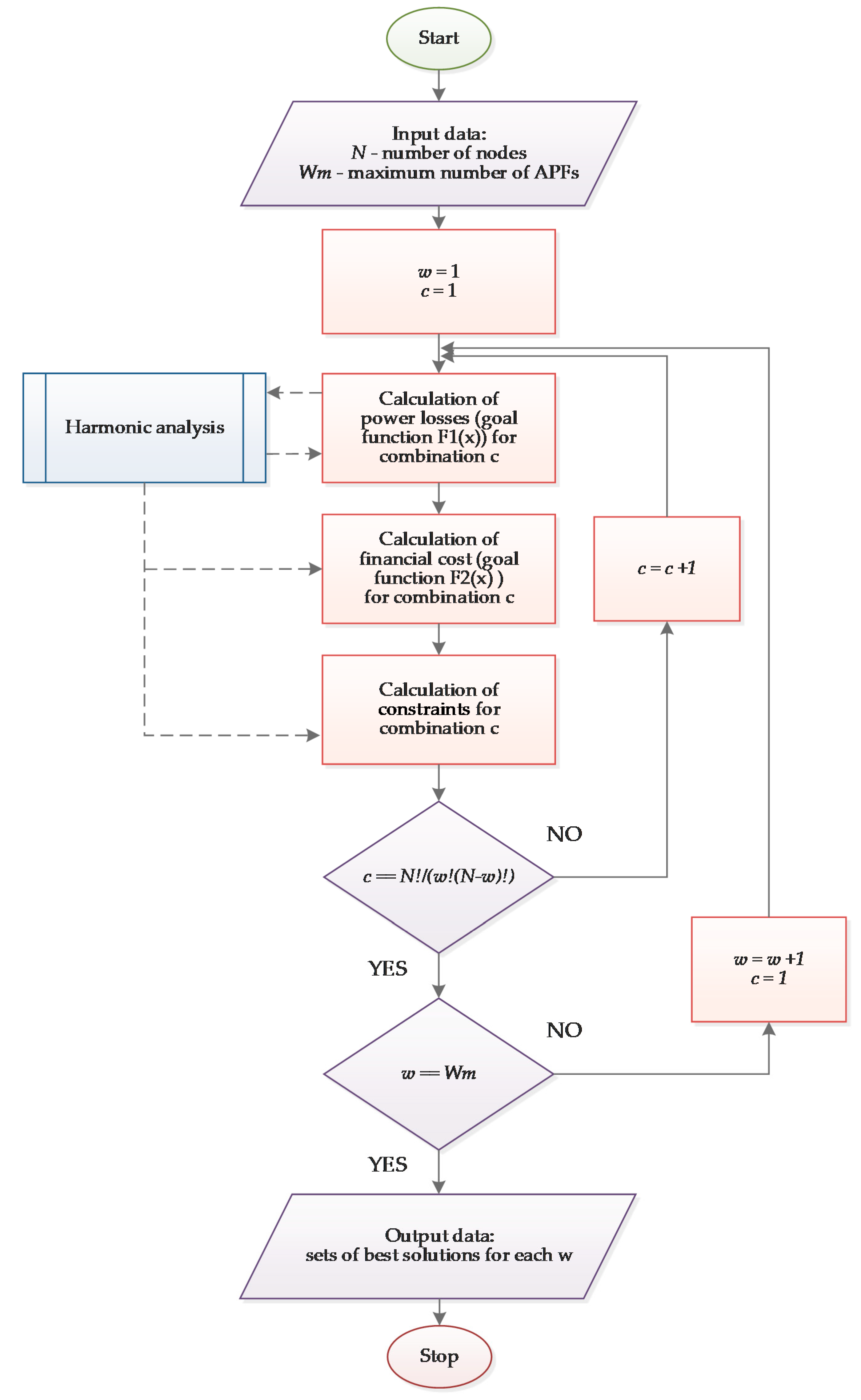
The proposed algorithm has been illustrated in Figure 9. Since the components of F(x) are competing—decreasing the power losses leads to increasing costs, there is no unique solution to this problem. Instead, the concept of Pareto optimality must be used to characterize the objectives. It expresses noninferior solutions for which an improvement in one objective function requires a degradation of the other. Finding the Pareto optima for the problem of APF allocation has been illustrated in an example presented in Chapter 5.
The function that reflects the cost of a single APF is discontinuous—some intervals of currents correspond to different costs being a result of an available set of APF nominal currents A = {, …, . Therefore, for a given APF, which has to be placed in the node w, we can define a subset of APF nominal currents Aw including elements such that:
The nominal current of the APF placed in the node w can be determined as the infimum of the subset Aw, i.e., .
The relation between APF price and nominal current is usually nonlinear, and it significantly influences the optimization results. An exemplary function, generated on the base of commercially available APFs price lists, has been shown in an example presented in Chapter 5.
Minimization of the cost must be accompanied by constraints that force acceptable and required by norms waveform distortions as well as power losses caused by higher harmonics. The most important one is:
where THDVmax denotes the maximum coefficient THD for voltage waveforms and usually is determined by standards, e.g., [50].
Finding a solution to the optimization problem enables us to answer the question: How many APFs, and in which nodes should they be installed in order to minimize the power losses and the financial cost, keeping the maximum voltage THD coefficient below the level imposed by the standards?
5. Case Study
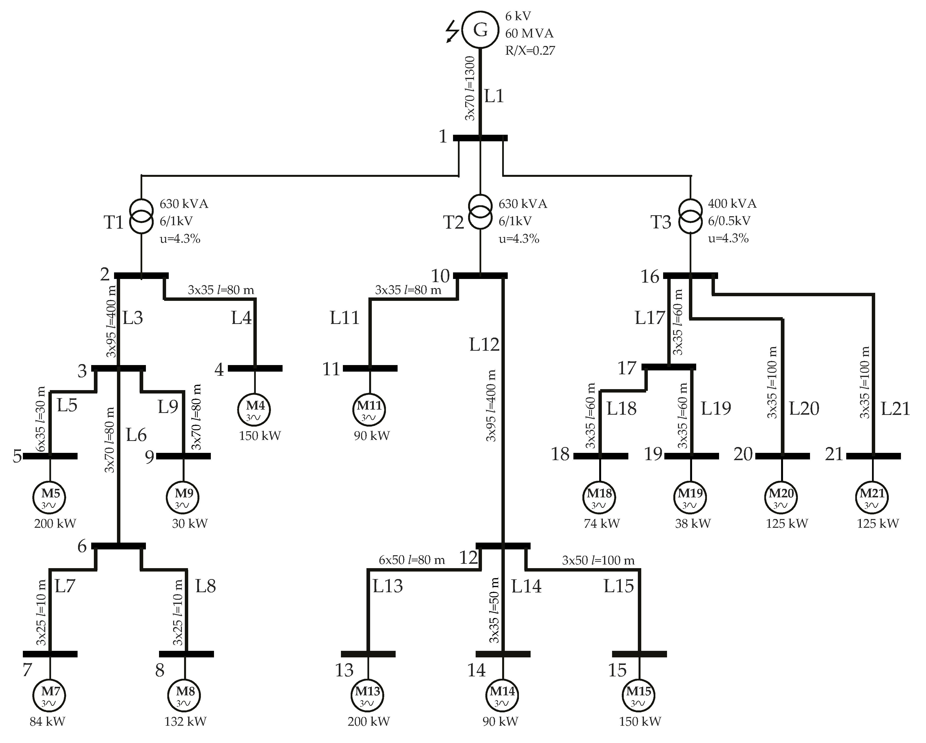
As an example for the optimization of the sizing and allocation of active power filters, a fragment of the real three-phase, three-wire low voltage power supply network located in one of the mines was selected. In such power systems, the load of transformers and power lines is essential in regard to safety and reliability motives. The significant length of cable lines causes voltage drop problems. The oversizing of the transformers and lines is not always possible for economic and technical (e.g., dimensions and weight of transformers) reasons. The power network shown in Figure 10 is composed of three transformers supplied by medium voltage line 6 kV AC. Two of the transformers form the 1 kV AC power network, whereas one-third of them form the 500 VAC network. These networks supply the mine’s machines, i.e., mine combines, fans, pumps, and conveyor belts with motors as executive elements. Currently, more and more of these motors are replaced by inverter drives. Therefore, in order to indicate potential problems in such networks and the possibility of using active filters, all drives are converter drives described by the models included in Chapter 3.2. The loads are three-phase balanced, so the entire network was modeled as an equivalent single-phase network.
It has been assumed that it is possible to add APF to the line over each node (except for node no. 1) of the low-voltage network. As a result, 20 possibilities of APF connection are achieved. The minimization of losses from higher harmonics has been taken as the basic optimization criterion. The additional condition is the voltage THD of no more than 5% attainment in all nodes. This supplementary condition causes that the optimal solution is sought only in cases where it is achieved. The nonideal APF with the efficiency characteristic shown in Figure 4, and 98% energy efficiency has been taken into consideration.
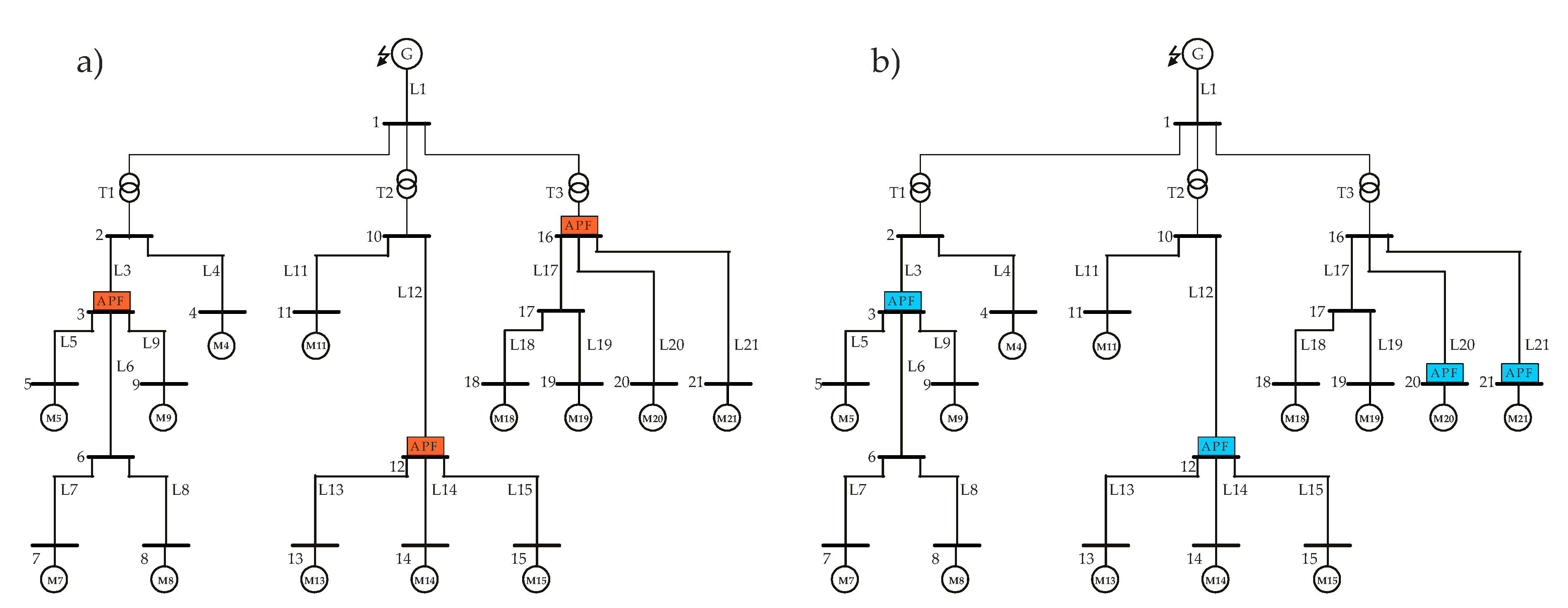
For example, the selection and placement optimization of one to six APFs systems has been determined. As it is shown in Table 5, only solutions with the application of three or more APFs can give the results with THD not higher than 5% in all nodes. The APF optimal connection places in the analyzed example of the power network for the case of three and four APFs are shown in Figure 11.
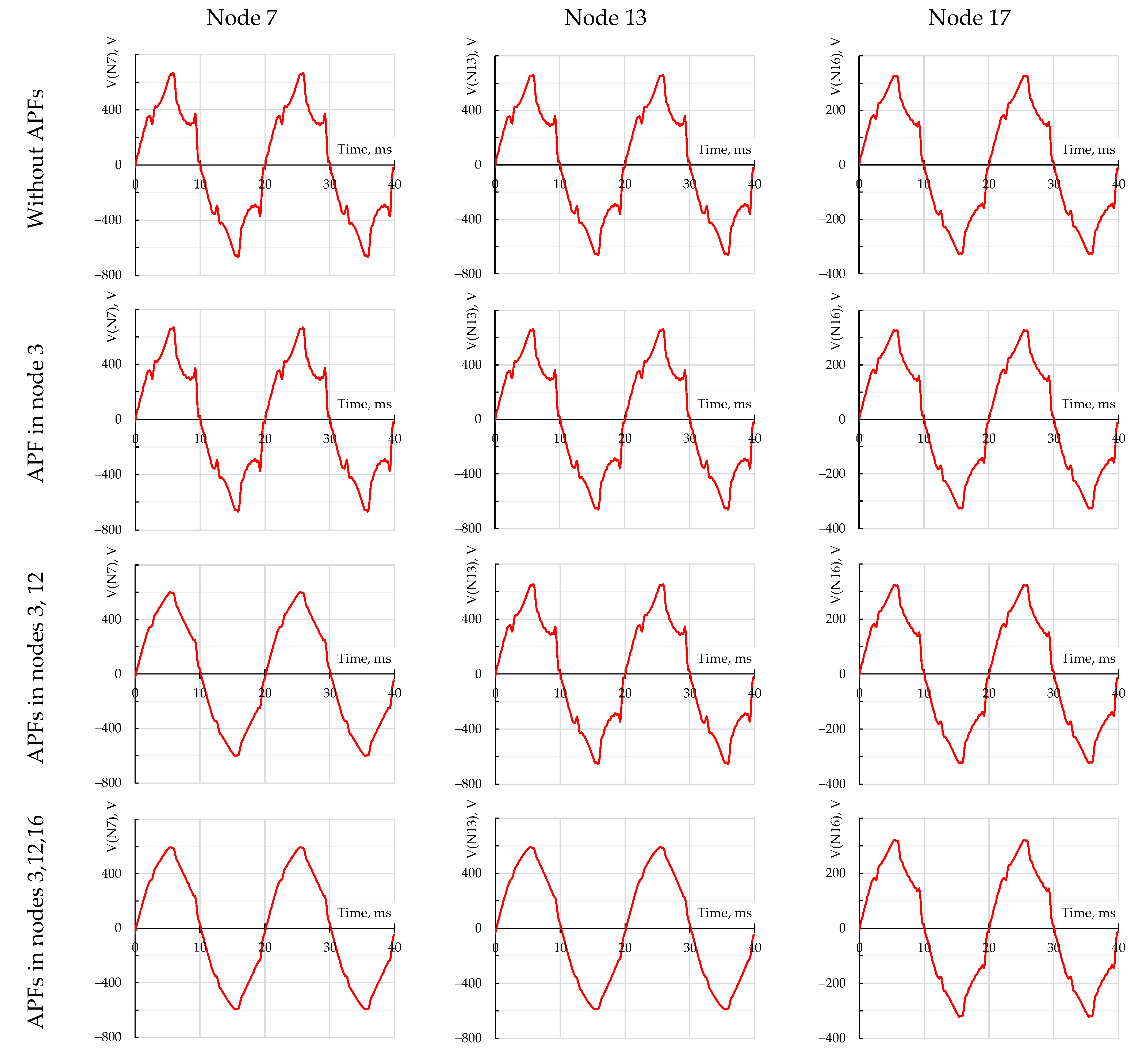
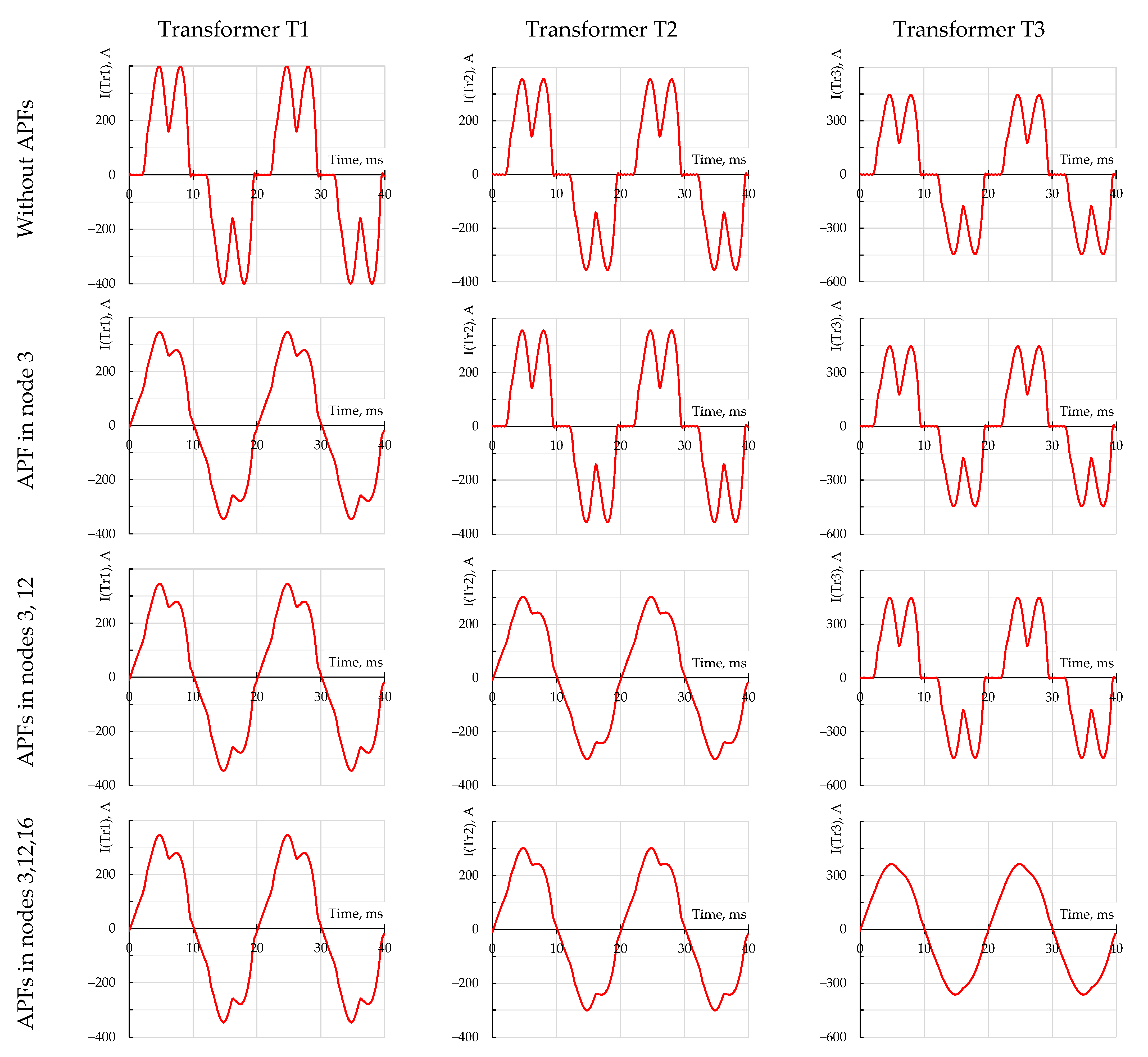
In the system without APF, the THD distortion can reach 18%. It is a result of the great length of the cable lines loaded with deformed current. The example of the voltage waveforms for the case of the system without APF and the system with one, two, and three APFs has been presented in Figure 12. Figure 13 shows the waveforms of the output currents for transformers in the same cases as the voltages in Figure 12. The THD factor of the currents in the case of three APFs for particular transformers was 12.2%, 9.2%, and 2.8%, respectively.
The results for the transformers, summarized in Table 6, are interesting, too. The particular values were calculated according to the definition:
- |ST|—output apparent power of the transformer,
- PT—output active power of the transformer,
- transformer output power factor:
- higher harmonics power losses of the transformer:
- total power losses of the transformer:
- percentage of losses:
The used model of the transformer allows us to take into account the eddy current losses for higher harmonics, which can be perceived while there is no APF connected. Then, the losses of the higher harmonics reach 36% of the total transformer losses. The active filter usage resulted in gaining the acceptable level of loss reduction. Furthermore, the reactive power compensation for the first harmonic leads to an output PF factor of all transformers close to unity even when only three APFs are used. From the transformer’s point of view, further adding APFs to the examined power network does not make much sense, because it does not reduce losses. As one can see, it is possible to reduce the total transformer losses by almost 30%. It is especially important in the mining environment because of the limited transformer cooling possibilities.
Table 7 shows the summary of the total losses related to a particular number of active filters. The coefficients are calculated according to the formulae:
- Source power factor:
- Higher harmonics power losses:
- Total power losses:
- Reduction of higher harmonics losses:
- Reduction of total power losses:
- Percentage of losses:
- Active power filter losses:
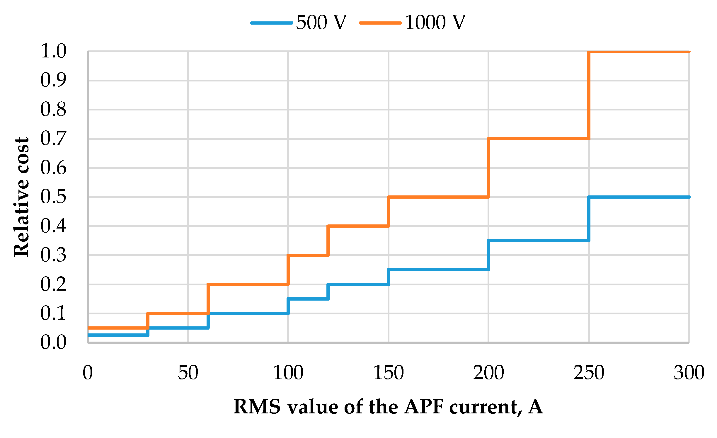
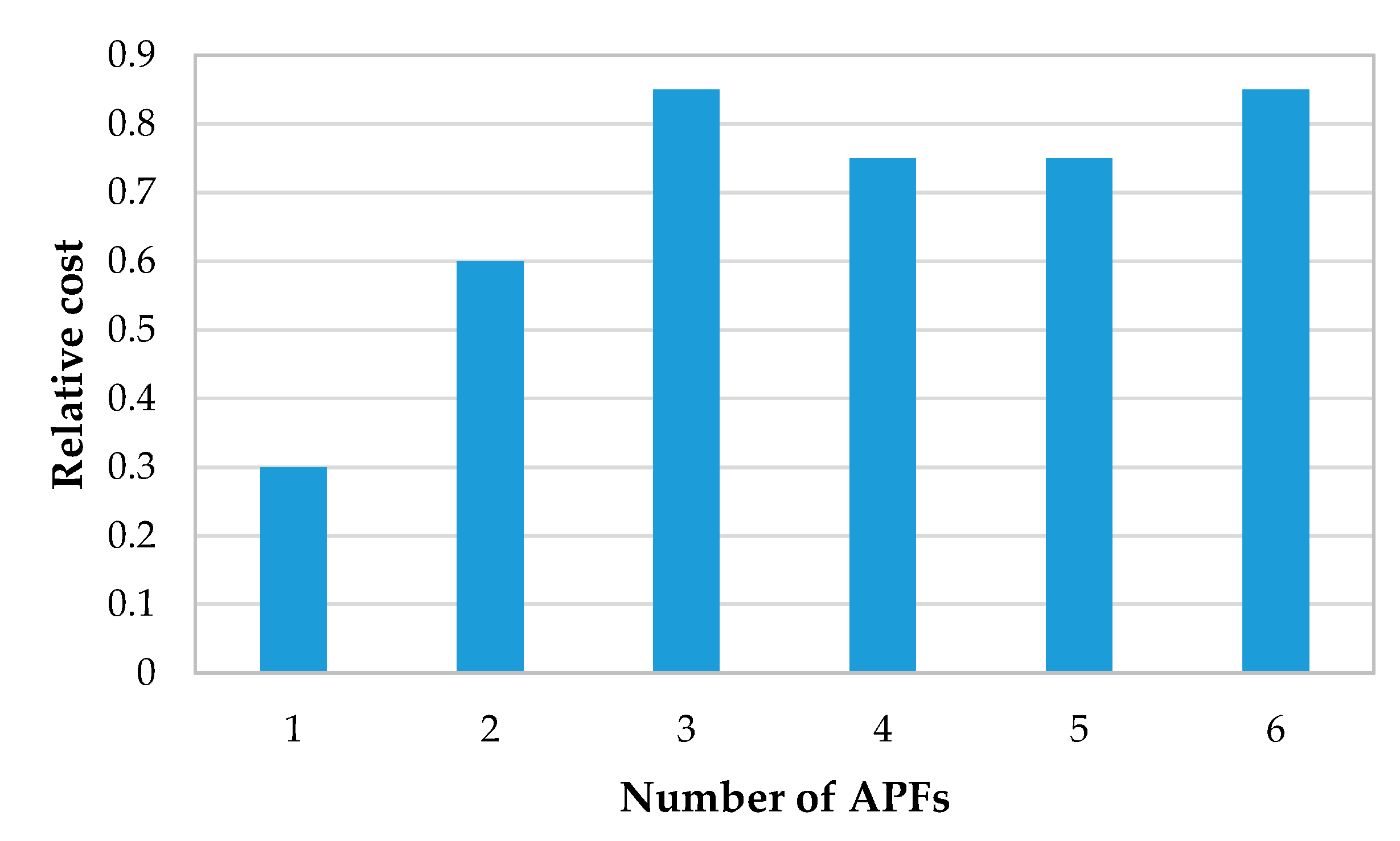
It is easy to notice that the reduction of higher harmonic losses and the improvement of the power factor (PF) of the generator depend on the number of active filters used in the system. However, taking into account that the real efficiency value of the APF model is 98%, it can be seen that adding more APFs to the network will not be associated with a further reduction of losses. The best losses reduction in comparison with the parameters of power network without APF has been reached in the case with four installed APFs. These results have been marked in green in Table 7. Interestingly, the total losses generated by the APFs and the cost of use of four filters are lower than that for three APFs. The analysis assumed the dependence of the cost on the APF RMS current value in accordance with the characteristics in Figure 14 (the most expensive APF is 100% of the cost). The relative cost of applying a particular number of APFs has been shown in Figure 15. The application of two less powerful APFs at nodes 20 and 21 proves to be more cost-effective than one APF at node 16.
Further results presented in Table 8 concern the time calculation of the optimization depending on the number of applied APFs. The increase in the number of connected APFs causes a significant increase in the number of possible cases. For the analyzed example, connecting six APFs in 20 possible nodes requires the calculation of 38,760 cases. The presented software shows a linear dependence of the calculation time on the number of cases. For the examined example, for which the dimension of the matrix A is 124 × 124, it was about 104 ms for a single case. For each of the cases, it is necessary to calculate the results for the circuit several times. This number results from the number of analyzed harmonics and the number of iterations for the fundamental harmonic. The average time of a single circuit calculation in this case was 0.6 ms.
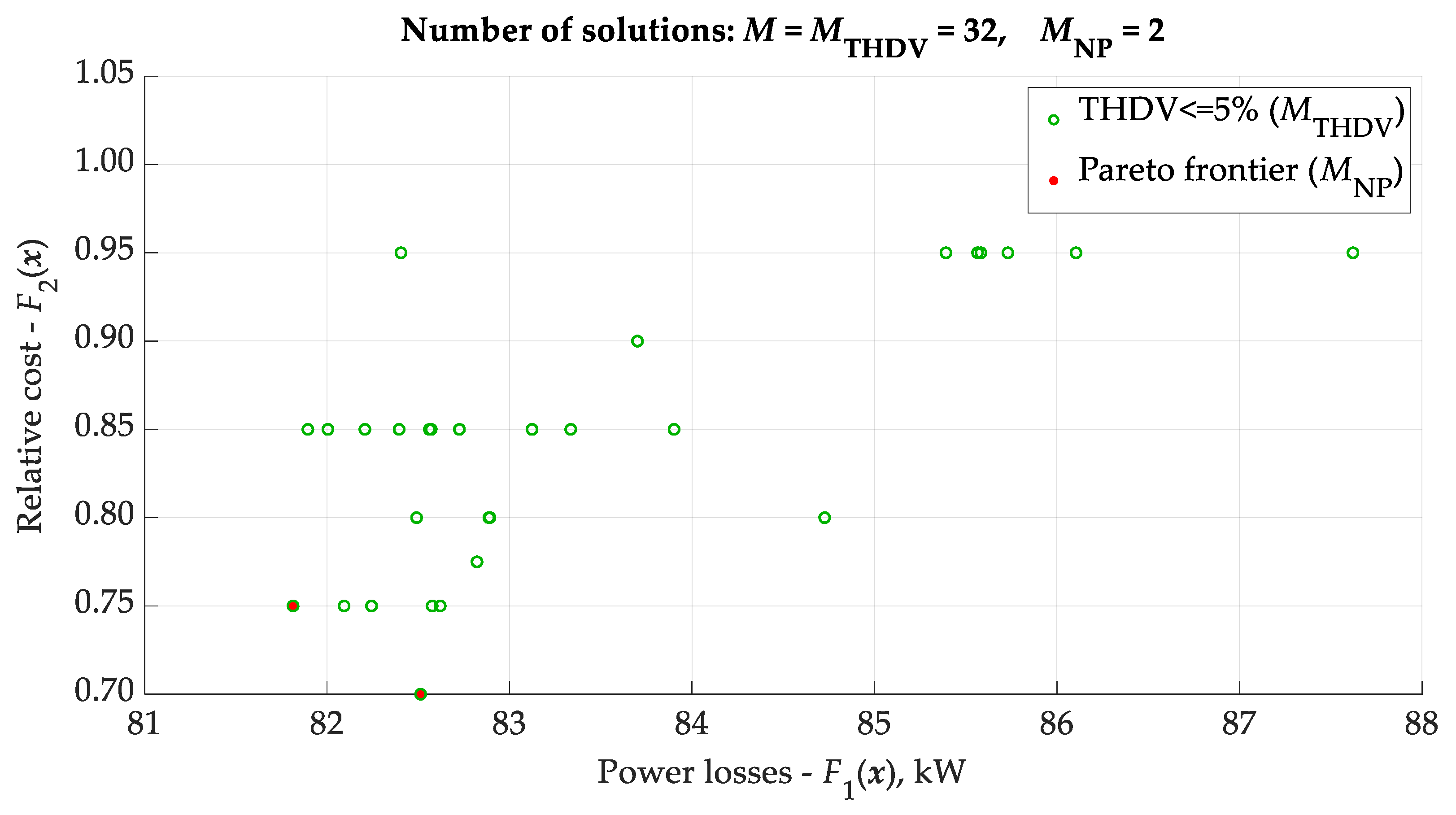
In order to illustrate the theoretical considerations presented in Chapter 4, for the case of four APFs in the system, all feasible solutions have been presented in Figure 16. As it can be read only for 32 solutions out of 4845 (see Table 8), the constraint (20) is fulfilled. Moreover, the Pareto frontier includes two solutions for which the vector of objective functions F given by (16) takes approximately the values [82.5; 0.70] and [81.8; 0.75]. Both solutions are optimal in the Pareto sense, and the choice of the one to be implemented can be based on other technical aspects, e.g., preferences in APF allocation in some nodes, or long-term analysis of the financial cost of each solution optimal in the Pareto sense.
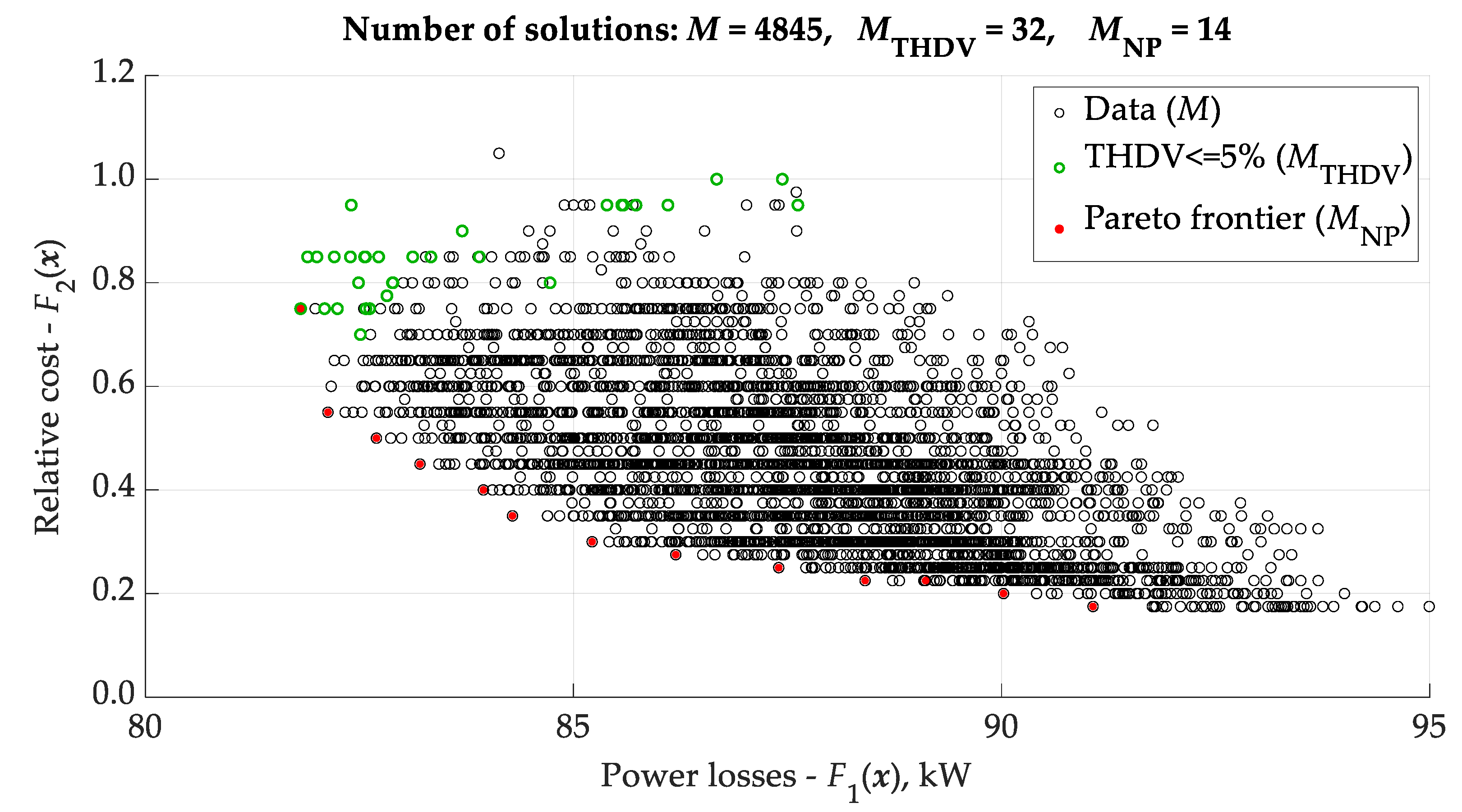
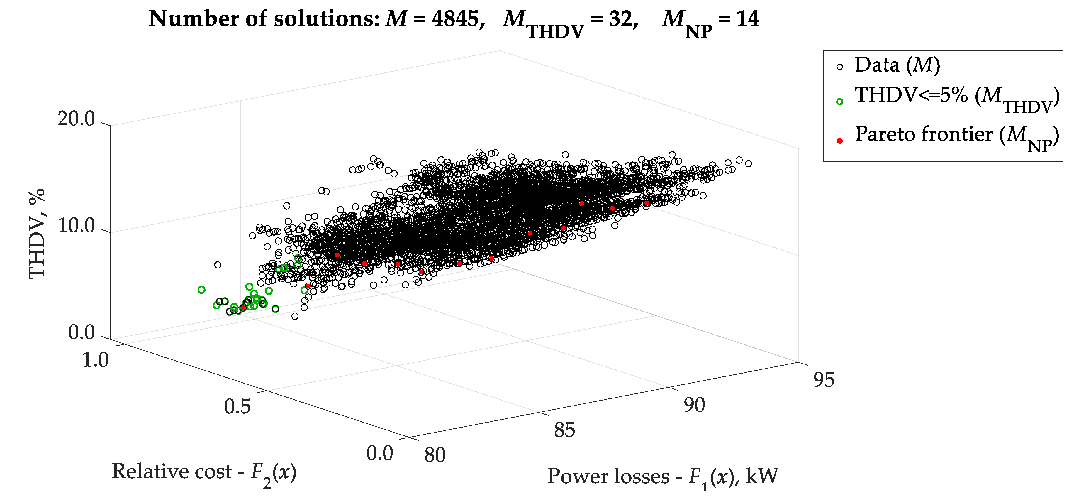
The deeper insight in this example can be reached if all solutions for four APFs are presented—see Figure 16. The Pareto frontier includes in this case 14 points that represent the optimum solutions for the unconstrained problem. The feasible points presented in Figure 16 have been also marked out in Figure 17. The same data have been used to show the solution in 3D space (see Figure 18).
6. Discussion
The paper presents the possibilities of the developed software for modeling and simulating power supply systems in the frequency domain. The use of frequency domain modeling and the appropriate construction of models allowed for the development of efficient and at the same time flexible software, in which it was possible to perform optimization tasks with a satisfactory performance despite the use of the Brute Force algorithm.
The presented examples show that the developed software allows for the construction of custom models of system components, as well as their efficient implementation, and the obtained results reflect the phenomena occurring in the analyzed system with good accuracy.
The developed software was used to optimize the allocation of active filters in the exemplary power supply system. Contrary to other works related to the optimization of the APFs allocation [3,4,5,6,7,8,9,10,11,12,13,14,15,16,17,18,19,20,21,22,23,24,25,26], the example considers a low-voltage network for which there are many APF solutions available on the market.
The applied APF model allows for the simulation of cases in which it is possible to reduce the efficiency of higher harmonics filtering and to take into account the losses generated by the APFs. Such a model much better reflects the real case, especially in terms of APFs efficiency (see Table 7). It turns out that in order to minimize the loss of active power, depending on the number of APFs used in the network, there is a certain optimum of the number of used APFs, and its further increase does not reduce losses despite the reduction of the THD coefficient in the network nodes (Table 5). The economic factor also turned out to be interesting for the analysis. From the analysis of the characteristics shown in Figure 17, it can be concluded that the solution next to the optimal one allows reducing the investment cost by over 26% with just a slight change in power losses and resignation from a strict limitation on voltage THD. This example shows that the appropriate software allows for an in-depth analysis of the possible solutions and the selection of the optimal one for a specific case, depending on the adopted restrictions, expected effects, and investment costs.
It is also worth mentioning the transformer model used in the presented simulations, in which the eddy current losses for higher harmonics were taken into account. As it was shown in Table 6, losses from higher harmonics of current are an important component of the total losses in the transformers, and their omission in the model would be a mistake considering the adopted optimization goal.
The achieved optimization times (see Table 8) with the similar number of nodes where APF systems can be connected (which means a similar number of combinations) were significantly lower than the times achieved in earlier works [31] (see Table 3). Despite the different sizes of the analyzed networks and different test environments, the undeniable advantage of the developed “pqs-core” software can be seen here.
Further work will focus on the possibility of using other known optimization algorithms that enable us to find global solutions to problems with multiple objectives and identify a Pareto front-like genetic algorithms or pattern search solvers, which may be necessary in the case of larger power systems. It is also planned to further expand the individual models of system elements and add new ones.
Author Contributions
Conceptualization, D.B., D.G., M.M., M.L., A.P.; methodology, D.B., D.G., M.M., M.L., A.P.; software, D.B., M.L.; validation, D.B., D.G., M.M., M.L., A.P.; formal analysis, D.G.; writing—original draft preparation, D.B., D.G., M.M., M.L., A.P.; writing—review and editing, D.B., D.G., M.M., M.L., A.P.; supervision, D.B., D.G. All authors have read and agreed to the published version of the manuscript.
Funding
This research was partly financed by the EU funding for 2014–2020 within Smart Growth Operational Programme.
Institutional Review Board Statement
Not applicable
Informed Consent Statement
Not applicable
Data Availability Statement
The data presented in this study are available on request from the corresponding author. The data are not publicly available due to at the date of publication, no data repository has been established yet.
Conflicts of Interest
The authors declare no conflict of interest.
Abbreviations
| THD | Total harmonic distortion |
| APF | Active power filter |
| HAPF | Hybrid active power filter |
| PSO | Particle swarm optimization |
| DEA | Differential evolution algorithm |
| GA | Genetic algorithm |
| RMS | Root mean square—effective value |
References
- Maciążek, M. Power theories applications to control active compensators. In Power Theories for Improved Power Quality; Benysek, G., Pasko, M., Eds.; Springer: London, UK, 2012; pp. 49–116. [Google Scholar]
- Buła, D.; Pasko, M. Model of hybrid active power filter in the frequency domain. In Analysis and Simulation of Electrical and Computer Systems; Gołębiowski, L., Mazur, D., Eds.; Springer: Berlin, Germany, 2011; pp. 15–26. [Google Scholar]
- Maciążek, M.; Grabowski, D.; Pasko, M. Active power filters-optimization of sizing and placement. Bull. Pol. Acad. Sci. Tech. Sci. 2013, 61, 847–853. [Google Scholar] [CrossRef] [Green Version]
- Grabowski, D.; Maciążek, M.; Pasko, M. Sizing of active power filters using some optimization strategies. COMPEL Int. J. Comput. Math. Electr. Electron. Eng. 2013, 32, 1326–1336. [Google Scholar] [CrossRef] [Green Version]
- Maciążek, M.; Grabowski, D.; Pasko, M. Genetic and combinatorial algorithms for optimal sizing and placement of active power filters. Int. J. Appl. Math. Comput. Sci. 2015, 25, 269–279. [Google Scholar] [CrossRef] [Green Version]
- Urrutia Ramos, F.; Cortes, J.; Torres, H.; Gallego, L.E.; Delgadillo, A.; Buitrago, L. Implementation of genetic algorithms in ATP for optimal allocation and sizing of active power line conditioners. In Proceedings of the IEEE/PES Transmission & Distribution Conference and Exposition, Latin America, Caracas, Venezuela, 8 August 2006; pp. 1–5. [Google Scholar]
- Dehghani, N.; Ziari, I. Optimal allocation of APLCs using genetic algorithm. In Proceedings of the 43rd International Universities Power Engineering Conference, Padova, Italy, 1 September 2008; pp. 1–4. [Google Scholar]
- Yan-song, W.; Hua, S.; Xue-min, L.; Jun, L.; Song-bo, G. Optimal allocation of the active filters based on the tabu algorithm in distribution network. In Proceedings of the International Conference on Electrical and Control Engineering, Wuhan, China, 25 June 2010; pp. 1418–1421. [Google Scholar]
- Ayoubi, M.; Hooshmand, R.A. A new fuzzy optimal allocation of detuned passive filters based on a Nonhomogeneous Cuckoo Search Algorithm considering resonance constraint. ISA Trans. 2019, 89, 186–197. [Google Scholar] [CrossRef]
- Carpinelli, G.; Russo, A.; Varilone, P. Active filters: A multi-objective approach for the optimal allocation and sizing in distribution networks. In Proceedings of the International Symposium on Power Electronics, Electrical Drives, Automation and Motion (SPEEDAM), Ischia, Italy, 18–20 June 2014; pp. 1201–1207. [Google Scholar]
- Ziari, I.; Jalilian, A. Optimal placement and sizing of multiple APLCs using a modified discrete PSO. Int. J. Electr. Power Energy Syst. 2012, 43, 630–639. [Google Scholar] [CrossRef]
- Shivaiea, M.; Salemniab, A.; Amelib, M.T. A multi-objective approach to optimal placement and sizing of multiple active power filters using a music-inspired algorithm. Appl. Soft Comput. 2014, 22, 189–204. [Google Scholar] [CrossRef]
- Farhoodneaa, M.; Mohameda, A.; Shareefa, H.; Zayandehroodib, H. Optimum placement of active power conditioner in distribution systems using improved discrete firefly algorithm for power quality enhancement. Appl. Soft Comput. 2014, 23, 249–258. [Google Scholar] [CrossRef]
- Lakum, A.; Mahajan, V. Optimal placement and sizing of multiple active power filters in radial distribution system using grey wolf optimizer in presence of nonlinear distributed generation. Electr. Power Syst. Res. 2019, 173, 281–290. [Google Scholar] [CrossRef]
- Chen, Y.; Chen, W.; Yang, R.; Li, Z. Optimal allocation method of hybrid active power filters in active distribution networks based on differential evolution algorithm. J. Power Electron. 2019, 19, 1289–1302. [Google Scholar]
- El-Arwash, H.M.; Azmy, A.M.; Rashad, E.M. A GA-based initialization of PSO for optimal APFS allocation in water desalination plant. In Proceedings of the Nineteenth International Middle East Power Systems Conference (MEPCON), Cairo, Egypt, 19 December 2017; pp. 1378–1384. [Google Scholar]
- Milovanović, M.; Radosavljević, J.; Klimenta, D.; Perovic, B. GA-based approach for optimal placement and sizing of passive power filters to reduce harmonics in distorted radial distribution systems. Electr. Eng. 2019, 101, 787–803. [Google Scholar] [CrossRef]
- Mojtaba Shivaie, M.; Salemnia, A.; Ameli, M.T. Optimal multi-objective placement and sizing of passive and active power filters by a fuzzy-improved harmony search algorithm. Electr. Energy Syst. 2015, 25, 520–546. [Google Scholar]
- Far, A.M.; Foroud, A.A. Cost-effective optimal allocation and sizing of active power filters using a new fuzzy-MABICA method. IETE J. Res. 2016, 62, 307–322. [Google Scholar]
- Moradifar, A.; Foroud, A.A. A hybrid fuzzy DIAICA approach for cost-effective placement and sizing of APFs. IETE Tech. Rev. 2017, 34, 579–589. [Google Scholar] [CrossRef]
- Carpinelli, G.; Proto, D.; Russo, A. Optimal planning of active power filters in a distribution system using trade-off/risk method. IEEE Trans. Power Deliv. 2017, 32, 841–851. [Google Scholar] [CrossRef]
- Subramani, C.; Jimoh, A.A.; Dash, S.S.; Harishkiran, S. PSO application to optimal placement of UPFC for loss minimization in power system. In Advances in Intelligent Systems and Computing, Proceedings of the 2nd International Conference on Intelligent Computing and Applications, Amsterdam, Netherlands, 22 February 2015; Springer: Singapore, 2017; pp. 223–230. [Google Scholar]
- Chakeri, V.; Hagh, M.T. Optimal allocation of the distributed active filters based on total loss reduction. Int. J. Smart Electr. Eng. 2017, 6, 171–175. [Google Scholar]
- Sedighizadeh, M.; Doyran, R.V.; Rezazadeh, A. Optimal simultaneous allocation of passive filters and distributed generations as well as feeder reconfiguration to improve power quality and reliability in microgrids. J. Clean. Prod. 2020, 265, 121629. [Google Scholar] [CrossRef]
- Li, D.; Wu, Z.; Zhao, B.; Zhang, X.; Zhang, L. An Adaptive active power optimal allocation strategy for power loss minimization in islanded microgrids. In Proceedings of the 45th Annual Conference of the IEEE Industrial Electronics Society (IECON), Lisbon, Portugal, 14–17 October 2019; pp. 292–297. [Google Scholar]
- Doyran, R.V.; Sedighizadeh, M.; Rezazadeh, A.; Alavi, S.M.M. Optimal allocation of passive filters and inverter based DGs joint with optimal feeder reconfiguration to improve power quality in a harmonic polluted microgrid. Renew. Energy Focus 2020, 32, 63–78. [Google Scholar] [CrossRef]
- Baggini, A. Handbook of Power Quality; John Wiley & Sons: Hoboken, NJ, USA, 2008. [Google Scholar]
- Buła, D.; Lewandowski, M. Steady state simulation of a distributed power supplying system using a simple hybrid time-frequency model. Appl. Math. Comput. 2018, 319, 195–202. [Google Scholar] [CrossRef]
- Sowa, M.; Majka, Ł. Ferromagnetic core coil hysteresis modeling using fractional derivatives. Nonlinear Dyn. 2020, 101, 775–793. [Google Scholar] [CrossRef]
- Power Systems Analytical Software Tools. Available online: https://www.itee.uq.edu.au/pssl/drupal7_with_innTheme/index.html@q=node%252F34.html (accessed on 4 November 2020).
- Maciążek, M.; Pasko, M. Optimum allocation of active power filters in large supply systems. Bull. Pol. Acad. Sci. Tech. Sci. 2016, 64, 37–44. [Google Scholar] [CrossRef] [Green Version]
- Grabowski, D.; Walczak, J. Strategies for optimal allocation and sizing of active power filters. In Proceedings of the 11th International Conference on Environment and Electrical Engineering (EEEIC), Venice, Italy, 18–25 May 2012; pp. 1–4. [Google Scholar]
- Buła, D.; Lewandowski, M. Comparison of Frequency Domain and Time Domain Model of a Distributed Power Supplying System with Active Power Filters (APFs). Appl. Math. Comput. 2015, 267, 771–779. [Google Scholar] [CrossRef]
- Lewandowski, M.; Walczak, J. Current Spectrum Estimation Using Prony’s Estimator and Coherent Resampling. COMPEL Int. J. Comput. Math. Electr. Electron. Eng. 2014, 33, 989–997. [Google Scholar] [CrossRef]
- DeCarlo, R.A.; Lin, P.M. Linear Circuit Analysis: Time Domain, Phasor and Laplace Transform Approaches; Oxford University Press: New York, NY, USA, 2001. [Google Scholar]
- Java Matrix Benchmark. Available online: https://lessthanoptimal.github.io/Java-Matrix-Benchmark/ (accessed on 26 October 2020).
- Borwain, J.M.; Lewis, A.S. Convex Analysis and Nonlinear Optimization: Theory and Examples; Springer: New York, NY, USA, 2000; pp. 179–213. [Google Scholar]
- Wildi, T. Electrical Machines, Drives and Power Systems, 5th ed.; Prentice-Hall: Englewood Cliffs, NJ, USA, 2000. [Google Scholar]
- Faiz, J.; Ghazizadeh, M.; Oraee, H. Derating of transformers under non-linear load current and non-sinusoidal voltage—An overview. IET Electron. Power Appl. 2015, 9, 486–495. [Google Scholar] [CrossRef]
- Elmoudi, A.; Lehtonen, M.; Nordman, H. Effect of harmonics on transformers loss of life. In Proceedings of the 2006 IEEE International Symposium on Electrical Insulation, Toronto, ON, Canada, 11–14 June 2006; pp. 408–411. [Google Scholar]
- Dugan, R.C.; McGranaghan, M.F.; Santoso, S.; Beaty, H.W. Electrical Power Systems Quality, 2nd ed.; McGraw-Hill: New York, NY, USA, 2003. [Google Scholar]
- Sindhu, M.R.; Jisma, M.; Maya, P.; Krishnapriya, P.; Vivek Mohan, M. Optimal placement and sizing of harmonic and reactive compensators in interconnected systems. In Proceedings of the 15th IEEE India Council International Conference (INDICON), Coimbatore, India, 16–18 December 2018; pp. 1–6. [Google Scholar]
- Yang, Z.; Zhuo, F.; Tao, R.; Zhang, Z.; Yi, G.; Wang, M.; Zhu, C. Implementation of multi-objective particle swarm optimization in distribution network for high-efficiency allocation and sizing of SAPFs. In Proceedings of the 22nd International Conference on Electrical Machines and Systems (ICEMS), Harbin, China, 11–14 August 2019; pp. 1–5. [Google Scholar]
- Moradifar, A.; Soleymanpour, H.R. A fuzzy based solution for allocation and sizing of multiple active power filters. J. Power Electron. 2012, 12, 830–841. [Google Scholar] [CrossRef] [Green Version]
- Keypour, R.; Seifi, H.; Yazdian-Varjani, A. Genetic based algorithm for active power filter allocation and sizing. Electr. Power Syst. Res. 2004, 71, 41–49. [Google Scholar] [CrossRef]
- Hong, Y.-Y.; Chang, Y.-K. Determination of locations and sizes for active power line conditioners to reduce harmonics in power systems. IEEE Trans. Power Deliv. 1996, 11, 1610–1617. [Google Scholar] [CrossRef]
- Grabowski, D.; Maciążek, M. Cost effective allocation and sizing of active power filters using genetic algorithms. In Proceedings of the 12th Int. Conf. on Environment and Electrical Engineering (EEEIC), Wrocław, Poland, 5–8 May 2013; pp. 467–472. [Google Scholar]
- Lewandowski, M.; Walczak, J. Comparison of classic and optimization approach to active power filters sizing and placement. COMPEL Int. J. Comput. Math. Electr. Electron. Eng. 2014, 33, 1877–1890. [Google Scholar] [CrossRef]
- Maciążek, M.; Grabowski, D.; Pasko, M.; Lewandowski, M. Compensation based on active power filters-the cost minimization. Appl. Math. Comput. 2015, 267, 648–654. [Google Scholar] [CrossRef]
- IEEE. Recommended practices and requirements for harmonic control in electric power systems. In IEEE Std519–2014 (Revision of IEEE Std 519–1992); IEEE: New York, NY, USA, 2014. [Google Scholar]
Figure 1.
General model of the pqs-core library.

Figure 2.
Harmonic analysis simulation algorithm.

Figure 3.
Model of active power filter.

Figure 4.
Example graph of harmonics reduction efficiency for an active power filter.

Figure 5.
Model of nonlinear load.

Figure 6.
Example current waveform and harmonic spectrum for nonlinear load.

Figure 7.
Model of a transformer.

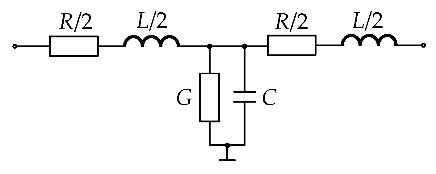
Figure 8.
Used model of the line.

Figure 9.
Block diagram of the combinatorial optimization algorithm for active power filter (APF) sizing and allocation.
Figure 9.
Block diagram of the combinatorial optimization algorithm for active power filter (APF) sizing and allocation.

Figure 10.
Diagram of the power network.

Figure 11.
The places of the optimal connection of the APFs devices in case of (a) three APFs, (b) four APFs.
Figure 11.
The places of the optimal connection of the APFs devices in case of (a) three APFs, (b) four APFs.

Figure 12.
Example of voltage waveforms of nodes 7, 13, and 16 for the cases of the system without APF and the system with one, two, and three APFs.
Figure 12.
Example of voltage waveforms of nodes 7, 13, and 16 for the cases of the system without APF and the system with one, two, and three APFs.

Figure 13.
Current waveforms for particular transformers without APF and the system with one, two, and three APFs.
Figure 13.
Current waveforms for particular transformers without APF and the system with one, two, and three APFs.

Figure 14.
The assumed relative cost of the APF depending on the current and rated voltage.

Figure 15.
The relative cost of using APF systems when optimally placed.

Figure 16.
Objective function values for all feasible solutions in the case of four APFs installed in the system (MTHDV—number of feasible solutions, MNP—number of noninferior points).
Figure 16.
Objective function values for all feasible solutions in the case of four APFs installed in the system (MTHDV—number of feasible solutions, MNP—number of noninferior points).

Figure 17.
Objective function values for all solutions in the case of four APFs installed in the system (M—total number of solutions, MTHDV—number of feasible solutions, MNP—number of noninferior points).
Figure 17.
Objective function values for all solutions in the case of four APFs installed in the system (M—total number of solutions, MTHDV—number of feasible solutions, MNP—number of noninferior points).

Figure 18.
Objective function and THDV values for all solutions in the case of four APFs installed in the system (M—total number of solutions, MTHDV—number of feasible solutions, MNP—number of noninferior points).
Figure 18.
Objective function and THDV values for all solutions in the case of four APFs installed in the system (M—total number of solutions, MTHDV—number of feasible solutions, MNP—number of noninferior points).


Table 1.
Comparison of the functionalities of free software for analyzing the operating state of power systems [30].
Table 1.
Comparison of the functionalities of free software for analyzing the operating state of power systems [30].
| Software | PF | OPF | TDS | HA | ETS |
|---|---|---|---|---|---|
| ATP | ☑ | ☑ | ☑ | ||
| MATPOWER | ☑ | ☑ | |||
| PCFLO | ☑ | ☑ | ☑ | ||
| PowerWorld | ☑ | ☑ | ☑ | ||
| PSAT | ☑ | ☑ | ☑ | ||
| PST | ☑ | ☑ | |||
| UWPFLOW | ☑ | ||||
| VST | ☑ | ☑ | ☑ |
Table 2.
Comparison of the functionalities of commercial software for analyzing the operating state of power systems [30].
Table 2.
Comparison of the functionalities of commercial software for analyzing the operating state of power systems [30].
| Software | PF | OPF | TDS | HA | ETS |
|---|---|---|---|---|---|
| CYME | ☑ | ☑ | ☑ | ☑ | ☑ |
| DigSILENT | ☑ | ☑ | ☑ | ☑ | ☑ |
| DINIS | ☑ | ||||
| DSATools | ☑ | ☑ | |||
| ETAP | ☑ | ☑ | ☑ | ☑ | |
| EUROSTAG | ☑ | ☑ | |||
| Mudpack | ☑ | ||||
| NEPLAN | ☑ | ☑ | ☑ | ☑ | |
| PowerWorld | ☑ | ☑ | ☑ | ||
| PSCAD | ☑ | ☑ | ☑ | ☑ | |
| PSS/E | ☑ | ☑ | ☑ | ||
| RTDS | ☑ | ☑ | ☑ | ||
| Simpow | ☑ | ☑ | ☑ | ||
| SimPowerSystems | ☑ | ☑ | ☑ | ☑ | |
| SKM PT | ☑ | ☑ | ☑ |
Where PF—Power Flow, OPF—Optimal Power Flow, TDS—Time Domain Simulation, HA—Harmonic Analysis, ETS –Electromagnetic Transient Studies.
Table 3.
Summary of calculation times for the optimization of the power supply system operation state with selected algorithms (GA—genetic algorithm, C—combinatorial algorithm).
Table 3.
Summary of calculation times for the optimization of the power supply system operation state with selected algorithms (GA—genetic algorithm, C—combinatorial algorithm).
| Algorithm | Compensator | Calculation Time |
|---|---|---|
| GA | APF | 2 h 15 m |
| GA | HAPF | 2 h 16 m |
| C | APF | 145 h 36 m |
| C | HAPF | 140 h 10 m |
Table 4.
Comparison of time in seconds of solving a system of complex equations (Intel Core i5-3210M, Win10_64, Java). 8).
Table 4.
Comparison of time in seconds of solving a system of complex equations (Intel Core i5-3210M, Win10_64, Java). 8).
| Number of Variables | 50 | 100 | 200 | 400 | 800 | 1600 | Algorithm | |
|---|---|---|---|---|---|---|---|---|
| Library | Apache Commons Math 3.6.1 | 0.023 | 0.045 | 0.307 | 1.154 | 9.251 | 84.01 | LU decomposition |
| ojAlgo 45.1 | 0.047 | 0.088 | 0.157 | 0.509 | 2.064 | 17.76 | ComplexMatrix.solve | |
| EJML 0.34 | 0.015 | 0.023 | 0.038 | 0.105 | 0.503 | 3.308 | LU decomposition | |
| Matlab 2010a | 0.00023 | 0.00090 | 0.0032 | 0.019 | 0.118 | 0.791 | X = B\A | |
| Scilab 6.0.1 | 0.00031 | 0.00067 | 0.0037 | 0.012 | 0.067 | 0.474 | X = B\A |
Table 5.
Voltage THD factors for particular nodes for optimal placement from one to six APFs.
| No. of APFs | 0 | 1 | 2 | 3 | 4 | 5 | 6 | |
|---|---|---|---|---|---|---|---|---|
| Nodes with APF | - | 3 | 3, 12 | 3, 12, 16 | 3, 12, 20, 21 | 3, 4, 12, 20, 21 | 3, 4, 12, 17, 20, 21 | |
| Above | Node | Voltage THD, % | ||||||
| G | 1 | 4.1 | 3.0 | 1.8 | 1.0 | 1.2 | 0.8 | 0.6 |
| T1 | 2 | 13.5 | 5.9 | 4.8 | 3.9 | 4.2 | 1.6 | 1.3 |
| 3 | 17.6 | 6.4 | 5.2 | 4.3 | 4.6 | 1.9 | 1.6 | |
| 4 | 18.1 | 6.3 | 5.6 | 4.7 | 5.0 | 2.2 | 2.0 | |
| 5 | 13.9 | 6.6 | 5.1 | 4.2 | 4.5 | 1.6 | 1.3 | |
| 6 | 17.8 | 6.8 | 5.4 | 4.5 | 4.8 | 2.0 | 1.8 | |
| 7 | 18.1 | 6.8 | 5.6 | 4.7 | 5.0 | 2.3 | 2.0 | |
| 8 | 18.1 | 6.8 | 5.6 | 4.7 | 5.0 | 2.3 | 2.0 | |
| 9 | 17.8 | 6.5 | 5.3 | 4.4 | 4.7 | 2.0 | 1.7 | |
| T2 | 10 | 12.5 | 11.3 | 3.8 | 3.0 | 3.2 | 2.8 | 2.6 |
| 11 | 16.5 | 11.5 | 4.2 | 3.3 | 3.6 | 3.2 | 2.9 | |
| 12 | 12.7 | 15.3 | 4.0 | 3.1 | 3.4 | 3.0 | 2.7 | |
| 13 | 16.9 | 15.7 | 4.6 | 3.7 | 4.0 | 3.6 | 3.3 | |
| 14 | 16.6 | 15.4 | 4.3 | 3.4 | 3.7 | 3.3 | 3.0 | |
| 15 | 16.9 | 15.7 | 4.6 | 3.7 | 4.0 | 3.5 | 3.2 | |
| T3 | 16 | 12.4 | 11.2 | 10.1 | 1.6 | 4.2 | 3.8 | 1.2 |
| 17 | 13.1 | 11.9 | 10.8 | 2.2 | 4.9 | 4.4 | 1.3 | |
| 18 | 13.4 | 12.2 | 11.0 | 2.5 | 5.0 | 4.7 | 1.5 | |
| 19 | 13.4 | 12.2 | 11.0 | 2.5 | 5.0 | 4.7 | 1.5 | |
| 20 | 13.8 | 12.6 | 11.4 | 2.8 | 4.4 | 4.0 | 1.3 | |
| 21 | 13.8 | 12.6 | 11.4 | 2.8 | 4.4 | 4.0 | 1.3 | |
Table 6.
Summary results for transformers without APF and optimally placed from one to six APFs.
| No. of APF | 0 | 1 | 2 | 3 | 4 | 5 | 6 |
|---|---|---|---|---|---|---|---|
| Transformer T1 | |||||||
| |ST|, kVA | 618 | 569 | 571 | 572 | 572 | 569 | 569 |
| PT, kW | 546 | 562 | 564 | 565 | 564 | 569 | 569 |
| PFT | 0.88 | 0.99 | 0.99 | 0.99 | 0.99 | 1.00 | 1.00 |
| PTHL, W | 2920 | 299 | 295 | 295 | 295 | 17 | 17 |
| PTTL, W | 10,471 | 7617 | 7634 | 7649 | 7644 | 7371 | 7375 |
| PTTL% | 1.92% | 1.36% | 1.35% | 1.35% | 1.36% | 1.30% | 1.30% |
| Transformer T2 | |||||||
| |ST|, kVA | 550 | 550 | 506 | 507 | 507 | 507 | 507 |
| PT, kW | 487 | 488 | 502 | 504 | 503 | 504 | 504 |
| PFT | 0.89 | 0.89 | 0.99 | 0.99 | 0.99 | 0.99 | 0.99 |
| PTHL, W | 2308 | 2323 | 133 | 133 | 133 | 133 | 133 |
| PTTL, W | 8774 | 8791 | 6424 | 6436 | 6432 | 6437 | 6441 |
| PTTL% | 1.80% | 1.80% | 1.28% | 1.28% | 1.28% | 1.28% | 1.28% |
| Transformer T3 | |||||||
| |ST|, kVA | 345 | 345 | 345 | 316 | 318 | 319 | 316 |
| PT, kW | 305 | 306 | 307 | 316 | 313 | 314 | 316 |
| PFT | 0.88 | 0.89 | 0.89 | 1.00 | 0.98 | 0.98 | 1.00 |
| PTHL, W | 1599 | 1611 | 1607 | 9.5 | 214 | 214 | 9.5 |
| PTTL, W | 6437 | 6450 | 6463 | 4721 | 4927 | 4931 | 4726 |
| PTTL% | 2.11% | 2.11% | 2.11% | 1.49% | 1.57% | 1.57% | 1.50% |
Table 7.
Summary results for an example power network in the case without APF and optimally placed from one to six APFs.
Table 7.
Summary results for an example power network in the case without APF and optimally placed from one to six APFs.
| No. of APF | 0 | 1 | 2 | 3 | 4 | 5 | 6 |
|---|---|---|---|---|---|---|---|
| PF | 0.886 | 0.933 | 0.972 | 0.990 | 0.985 | 0.990 | 0.990 |
| PHL, W | 15,866 | 9710 | 4468 | 2468 | 1979 | 1413 | 951 |
| PTL, W | 98,088 | 90,535 | 84,215 | 82,203 | 81,750 | 80,750 | 80,269 |
| δHL | - | 39% | 72% | 84% | 88% | 91% | 94% |
| Case with 100% energy efficiency of APF | |||||||
| PTL% | 7.03% | 6.65% | 5.92% | 5.75% | 5.70% | 5.64% | 5.59% |
| δTL | - | 7.4% | 14.1% | 16.2% | 16.8% | 17.7% | 18.2% |
| Case with 98% energy efficiency of APF | |||||||
| PAPFL, W | - | 3737 | 7454 | 10,374 | 9418 | 10,773 | 11,680 |
| PTL% | 7.03% | 6.92% | 6.44% | 6.48% | 6.33% | 6.39% | 6.40% |
| δTL | - | 3.89% | 6.54% | 5.62% | 7.05% | 6.69% | 6.26% |
Table 8.
Comparison of optimization time depending on the number of applied APFs (i7-9750H, 16GB RAM, Win10, Java 8).
Table 8.
Comparison of optimization time depending on the number of applied APFs (i7-9750H, 16GB RAM, Win10, Java 8).
| No. of APFs | 1 | 2 | 3 | 4 | 5 | 6 |
|---|---|---|---|---|---|---|
| Possible cases | 20 | 190 | 1140 | 4845 | 15,504 | 38,760 |
| No. of calculations | 377 | 3242 | 19,346 | 82,164 | 262,624 | 654,373 |
| Time, s | 0.3 | 2 | 11 | 48 | 163 | 405 |
Publisher’s Note: MDPI stays neutral with regard to jurisdictional claims in published maps and institutional affiliations. |
© 2020 by the authors. Licensee MDPI, Basel, Switzerland. This article is an open access article distributed under the terms and conditions of the Creative Commons Attribution (CC BY) license (http://creativecommons.org/licenses/by/4.0/).
Share and Cite
MDPI and ACS Style
Buła, D.; Grabowski, D.; Lewandowski, M.; Maciążek, M.; Piwowar, A. Software Solution for Modeling, Sizing, and Allocation of Active Power Filters in Distribution Networks. Energies 2021, 14, 133. https://doi.org/10.3390/en14010133
AMA Style
Buła D, Grabowski D, Lewandowski M, Maciążek M, Piwowar A. Software Solution for Modeling, Sizing, and Allocation of Active Power Filters in Distribution Networks. Energies. 2021; 14(1):133. https://doi.org/10.3390/en14010133
Chicago/Turabian StyleBuła, Dawid, Dariusz Grabowski, Michał Lewandowski, Marcin Maciążek, and Anna Piwowar. 2021. "Software Solution for Modeling, Sizing, and Allocation of Active Power Filters in Distribution Networks" Energies 14, no. 1: 133. https://doi.org/10.3390/en14010133
Note that from the first issue of 2016, this journal uses article numbers instead of page numbers. See further details here.