Dynamic Behavior of Wind Turbine Generator Configurations during Ferroresonant Conditions


Department of Electrical, Electronics and Computer Engineering, University of KwaZulu-Natal, Durban 4001, South Africa
*
Author to whom correspondence should be addressed.
Energies 2019, 12(4), 639; https://doi.org/10.3390/en12040639
Submission received: 21 October 2018
/
Revised: 15 November 2018
/
Accepted: 16 November 2018
/
Published: 16 February 2019
(This article belongs to the Collection Wind Turbines)
Abstract
:In this paper the dynamic behavior of different wind turbine generator configurations including doubly fed induction generators (DFIG), squirrel cage induction generator (SCIG), wound rotor induction generator (WRIG), and permanent magnet synchronous generator (PMSG) under ferroresonant conditions of energization and de-energization was investigated using Simulink/MATLAB (version 2017B, MathWorks, Natick, MA, USA). The result showed that SCIG had the highest overvoltage of 10.1 PU during energization, followed by WRIG and PMSG, while the least was DFIG. During de-energization, PMSG had the highest overvoltage of 9.58 PU while WRIG had the least. Characterization of the ferroresonance was done using a phase plane diagram to identify the harmfulness of the ferroresonance existing in the system. It was observed that for most of the wind turbine configurations, a chaotic mode of ferroresonance exists for both energization and de-energization scenarios. Although overvoltage during energization for wind turbine generator configurations was higher than in the de-energization with an exception of PMSG, their phase plane diagrams showed that de-energization scenarios were more chaotic than energization scenarios. The study showed that WRIG was the least susceptible to ferroresonance while PMSG was the most susceptible to ferroresonance.
1. Introduction
During the last six decades, power produced from wind turbines has grown from 20 kW to 3 MW [1]. This increase has been caused by various modifications and developments undertaken to the Gedser wind turbine concept developed in 1957, which was the first wind turbine to produce 20 kW [1]. One such modification was the introduction of the variable pitch blade; another modification was the introduction of asynchronous generators with wound rotors. Furthermore, the use of synchronous generators as wind turbine generators to replace asynchronous generators was another concept that was introduced in 1993 [1]. The depletion of the ozone layer caused by the usage of conventional energy and the development of wind energy technology has increased the interest in power generation from wind energy to the grid. One of the developments in wind power has been the integration of power electronics and their control strategies. Different technological concepts of the wind turbine generators obtained were from different combinational configurations of generators, power electronics, and control strategies. These have provided solutions to contingencies that arose from grid connected wind energy resulting in improved system efficiency and effectiveness [1,2]. Four of the popular wind turbine generator configuration types are: doubly fed induction generators (DFIG), squirrel cage induction generator (SCIG), wound rotor induction generator (WRIG), and permanent magnet synchronous generator (PMSG).
With the increased implementation of wind energy to the grid, it is important to consider various limitations that could affect its full functionality. One such limitation is temporary overvoltage as a result of ferroresonance events on a wind farm. Ferroresonance may occur in the event of a disturbance in a circuit with a non-linear inductor, capacitor, and voltage source. Even though ferroresonance falls under temporary overvoltage with its frequency ranging from 0.1 Hz to 1 kHz, the undamped characteristics of its overvoltage have effects on the service life of the equipment [3,4,5]. Ferroresonance may occur on a wind farm since all the components and conditions facilitating its occurrence exist. However, it is anticipated that different configurations of wind turbine generator types could behave differently in an event of ferroresonance. Thus, in this paper, the dynamic behavior of four wind turbine types namely: DFIG, SCIG, WRIG and PMSG, were analyzed during ferroresonant events.
Some studies have analyzed the behavior of wind turbine generator configurations when subjected to disturbances [6,7,8,9,10,11]. Neto et al. carried out a dynamic analysis of a grid connected wind farm using ATP software. They considered three configurations: DFIG, SCIG, and PMSG, while evaluating their behavior during the occurrence of disturbances on the wind farm. The disturbances evaluated were wind speed disturbance, loss of transmission lines, and three phase faults. It was observed that DFIG was the least affected by the disturbances, followed by SCIG, and PMSG was the most affected by the disturbance [6]. Erlich and Shewarega carried out simulations of system dynamics on wind turbines. They observed the response of the control system to a three phase grid fault on DFIG and PMSG. The generic model and detailed quasi-stationary (QSS) model were compared for the purpose of accuracy. It was found that the voltage results for the QSS model was 50% of the pre-fault value [7]. Ekanayeke and Jenkins studied the response of DFIG, SCIG, and PSMG wind turbines to change in network frequency and concluded that PSMG and SCIG released kinetic energy of their rotating mass when the power frequency was reduced, while DFIG could reduce its speed via the controller as an inertia response [8]. Karaagac et al. conducted research on ferroresonance on a wind farm involving a power transformer, inductive voltage transformer, and capacitive voltage transformer. The simulation was performed using EMTP-RV and the wind turbines were modelled as DFIG. Finally, the characterization of the ferroresonance was done using spectral analysis [9]. Siahpoosh et al. also worked on the assessment of ferroresonance on a wind farm which was caused by the cut-in operation of the wind speed, earth fault at the LV side of the transformer, and three phase to earth fault on the MV busbar. It was observed that all these disturbances were cleared by 0.2 s after their occurrence [10]. Corea-Araujo et al. worked on ferroresonance on a power transformer connected to SCIG. They experimented on different configurations of the power transformer connected to the SCIG and found that the delta–delta configuration of the transformer did not yield ferroresonance while the other yielded [11].
In this paper, temporary overvoltage due to ferroresonance was investigated on DFIG, SCIG, WRIG, and PSMG. The major contributions of this study is that the behavior of different wind turbine configuration types were analyzed under ferroresonant conditions to evaluate which wind turbine generator exhibited the highest overvoltage, and characterization of the ferroresonance was done using the phase plane in order to identify which mode of ferroresonance existed on each wind turbine configuration. At the time of writing this paper and to the best our knowledge, no literature has evaluated and compared the behavior of wind turbine generator configurations when subjected to ferroresonance.
This paper is sectioned as follows: an introduction is presented in Section 1, which includes a brief background and highlights our contribution to the topic. Section 2 deals with modelling the SCIG, WRIG, DFIG, and PMSG wind turbines. Section 3 shows the results of all the wind turbine generators under ferroresonant conditions. Finally, Section 4 discusses the summary of results and Section 5 presents the conclusions of this paper.
2. Modelling of the Wind Turbine Generator Types
Simulink/MATLAB was used as the simulation tool in this study. The rotor of the wind turbine was connected to the wind turbine generator through the gear box, whose function is to match the speed of the turbine to that of the generator. The output voltage of the generator was 0.69 kV, which was connected either directly or via electronic converter to the step-up transformer rated 0.69/33 kV, 2 MVA, and then supplied to the load. Mechanical torque was obtained from the wind turbine which acted as the prime mover. The most commonly available wind turbine today is the horizontal axis wind turbine (HAWT) with three blades. The output power resulting from the turbine blade due to the kinetic energy of the wind is given as Equation (1):
where R is the radius of the wind blade; ρ is the density of the air; v is the wind speed; and Cp is the power coefficient of the turbine, which depends on tip speed ratio, λ, and pitch angle, β. The tip speed ratio is represented by Equation (2):
where is the angular velocity of the rotor.
2.1. Modelling of the Drive Train
The torque is transferred from the rotor to the generator shaft via the gear box. The gear box consists of a drive train system that converts the low rotational speed of the turbine shaft to high speed to drive the generator. The gear box was modelled as a two-mass model as in [12] and Equations (3)–(7) depict the transmission of rotational speed from the turbine shaft to the generator shaft:
where Jt and Jg are the inertial of turbine shaft and generator side; and are the turbine and generator speed; Tt and Tg are the aerodynamic and generator torque; and are the shaft torsion of the turbine and generator; Dm is the damping coefficient; Kgear is the gear ratio; Ks is the stiff coefficient of the drive; and Kt and Kg are the friction coefficient of the turbine and generator, respectively.
2.2. Modelling of the Induction Generators
The operation of induction generators can be easily explained in two axes, the d-q coordinate axis. The mathematical representations of the induction generator are expressed as the following equations:
where Vsd, Vsq are the stator voltages in the d and q axis, respectively; Vrd, Vrd are the rotor voltages in the d and q axis, respectively; are the stator and rotor resistances, respectively; are the stator and rotor inductances, respectively; , are the stator and rotor self-inductances, respectively; is the mutual inductance; , are the stator currents in the d and q axis, respectively; , are the rotor currents in the d and q axis, respectively; , are the angular velocity of the rotor and stator, respectively; , are the stator fluxes in the d and q axis, respectively; and , are the rotor fluxes in the d and q axis, respectively. The torque, active power, and reactive power generated by the generator can be obtained using Equations (18)–(20):
2.2.1. Modelling of the SCIG and WRIG Wind Turbine Configurations
The output current and voltage from the SCIG and WRIG are fed to the softer starter which reduces the start-up current. The start-up current could be eight times higher than the rated current and this could cause disruption in the grid network. The soft starter consists of two thyristors and a by-pass switch which are connected in anti-parallel for each phase [13]. The firing angle α of the thyristors can be set to achieve the desired voltage in the case where it ranges from zero degree to sixty degrees. A capacitor bank of 500 kVar connected in delta for the purpose of compensating the reactive power consumed by the generator at start-up was calculated using Equation (21):
Modelling of the SCIG Wind Turbine Configuration
SCIG is also regarded as a fixed speed wind turbine generator with a pre-set wind speed which it operates. It has the advantages of simplicity, cost effectiveness, and robustness [2]. The generator is connected to the step-up transformer via a soft starter and a capacitor bank as shown in Figure 1. In the case of sudden change in wind speed, the pitch controller controls the electrical power supplied to the load. Table 1 shows the SCIG wind turbine data used in the model.
Modelling of the WRIG Wind Turbine Configuration
The WRIG is similar to the SCIG in terms of construction, but their difference lies in the addition of a variable resistor to the rotor side of the generator as shown in Figure 2. The control of the generator is achieved at the rotor of the generator by controlling the rotor voltages through the variable resistor. It is more effective to connect the variable resistor through the power electronics device instead of using slip rings to reduce energy loss. The data of the WRIG is shown in Table 2.
2.2.2. Modelling of the DFIG Wind Turbine Configuration
This wind type is configured so that the rotor side is connected through a back-to-back converter to the tertiary side of the wind turbine transformer and slip rings to the grid side while the stator is connected directly to the grid. This allows the generator to operate with variable wind speed. The configuration of DFIG allows full control of the generator by controlling the rotor and grid current, which results in the control of the active and reactive power fed to the grid. Figure 3 shows the schematic diagram of DFIG; the back-to-back converter consists of a machine side converter (MSC) and grid side converter (GSC) connected through a DC link, and Table 3 shows the data for the DFIG wind turbine. Control of the back-to-back converter of DFIG was modelled according to [14,15,16].
Control of the DFIG Machine Side Converter
Control of the MSC of the DFIG is shown in Figure 4, and it is a full bridge rectifier consisting of six insulated-gate bipolar transistors (IGBTs), which is a rectifier transforming AC output from the wind generator to DC. The control strategy consists of maximum power point tracking (MPPT) which ensures that optimum output power of the rotor is delivered, pulse width modulation (PWM) which correlates the controlled signal to the signal of the converter, phase locked loop (PLL).
By making reference to the rotating stator field in the d-q coordinate axis and representing stator flux on the d-axis, hence:
Substituting Equation (22) into Equations (12) and (13) result in
Substituting Equations (23) and (24) into Equations (14) and (15), give the following equations:
where σ is the coefficient of dispersion for the generator. To obtain the compensations necessary for controlling the voltage output of the rotor, Equations (25)–(27) are substituted into Equations (10) and (11):
Control of the DFIG Grid Side Converter
Control of the DFIG grid side converter is shown in Figure 5. The outer control loop regulates the error correction of the voltage of the DC Link and input specified voltage, which gives the reference q-axis grid current Igqref.
Error correction of Igqref and Igq is done to give Igq*, and error correction of Igdref and Igd is done to give Igd*. The inner loop controls both Igq* and Igd* to give Vgq* and Vgd*, respectively. Both Vgq* and Vgd* are compensated by Vgq and Vgd, respectively, and decoupled by using a low pass filter. The resultant Vgq and Vgd are transformed to the abc coordinate axis and passed through the PWM block. The equation of the grid voltage in the dq coordinate axis related to the stator rotation field where Vsd = Vs and Vsq = 0 can be given in Equations (32) and (33):
2.3. Modelling of the PMSG Wind Turbine Configuration
This is a synchronous generator that is excited by a permanent magnet unlike inductor generators that consume excitation current at start up. This configuration allows the output of the generator to be sent directly to the grid through a back-to-back converter. It also operates on variable wind speed and the converters control the real and reactive power output. The schematic diagram and data of the PMSG are shown in Figure 6 and Table 4, respectively.
Output voltage from the PMSG stator in the d-q reference frame can be obtained using Equations (34) and (35) while the electrical torque, real power, and reactive power output of the PMSG can be obtained using Equations (36)–(38), respectively:
where Lsd and Lsq are the stator direct and quadrature inductances and ψf is the flux linkage.
Control of the PMSG Converter
Figure 7 shows the control of both the stator side converter (SSC) and GSC of the PSMG according to [17,18,19,20]. The SSC consists of three control loops (one outer control loop and two inner control loops). The outer control loop regulates the rotor speed with optimal angular velocity from the MPPT control, resulting in the reference q-axis current Isqref. Results of the error correction of Isqref and Isq are controlled by one of the inner loop controls to produce V*sq. On the other hand, the second inner loop control regulates the error correction of Isdref and Isd to give V*sd. Both V*sd and V*sq are compensated by Vsdref and Vsqref, respectively, as expressed in Equation (39). Resultant Vsd and Vsq are transformed into the abc coordinate axis and passed through the pulse width modulation (PWM) block.
The power flows through the DC link to the grid side converter. The grid voltage in the d-q reference frame is expressed as Equation (40):
2.4. Modelling of Wind Turbine Transformer
3. Results
A ferroresonant event was simulated for all of the wind turbine configurations by assuming that a nuisance operation of the circuit breaker connecting the wind turbine transformer to the grid occurred. Two scenarios were considered: a stuck pole during energization and the de-energization of the circuit breaker, however, this allowed two poles to operate. The time for the simulation was one second while the circuit breaker was operated for 0.6 s. The following subsections show the ferroresonance result measured at the low voltage side of the transformer of each wind turbine generator configuration.
3.1. Ferroresonance on the SCIG Wind Turbine
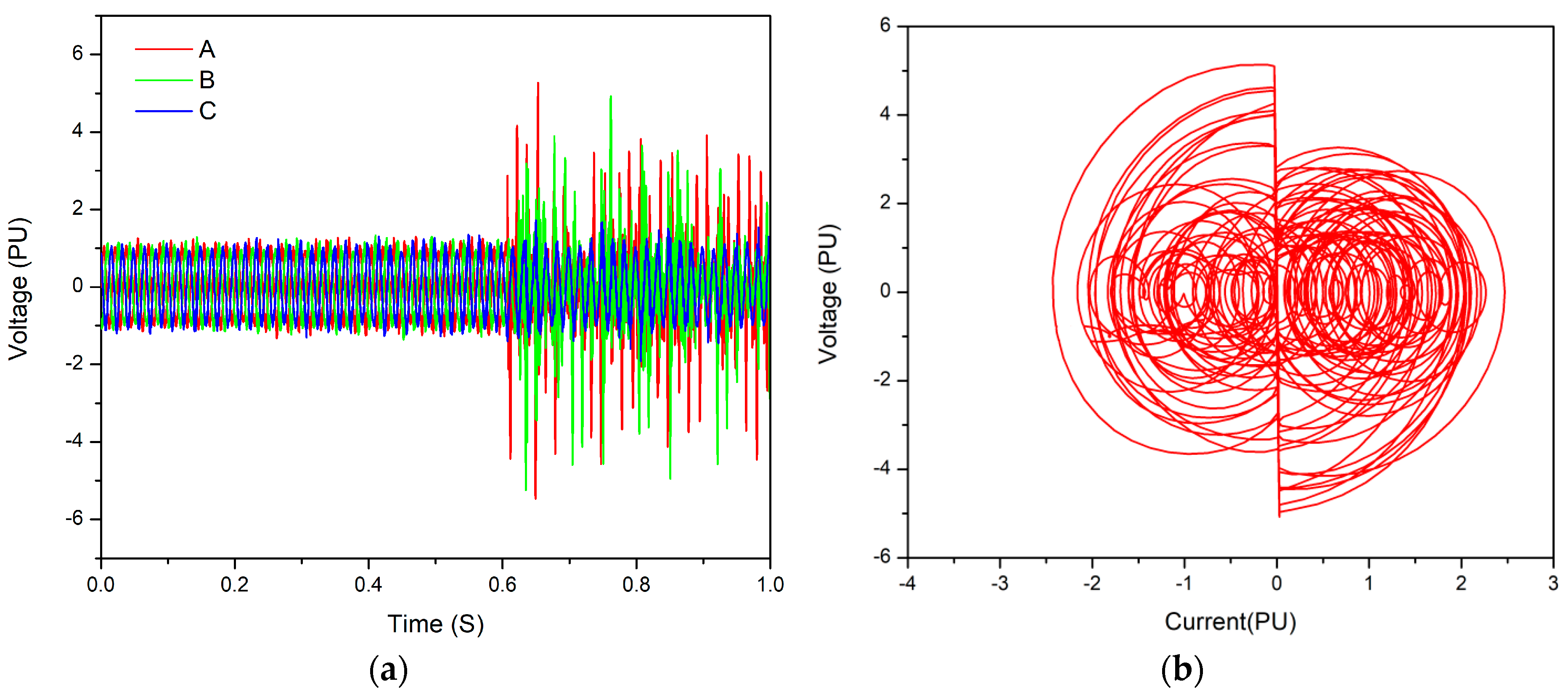
During energization of the SCIG to the grid, poles A and B were closed while pole C remained open. The interaction of the capacitor bank connected in delta with the wind turbine transformer caused ferroresonance phenomenon. Figure 8a shows the voltage waveform due to ferroresonance during the energization of SCIG with an overvoltage of 10.1 PU. Characterization of the ferroresonance was done using a phase plane diagram, resulting in a circular path form by the periodic signal of voltage and current. The non-regular circular path in Figure 8b depicts the ferroresonance in this system as chaotic since it did not follow either the periodic frequency nor any known frequency. However, during de-energization of SCIG, the overvoltage experienced was 5.71 PU as shown in Figure 9a. The chaotic mode also existed during de-energization as shown in Figure 9b. Even though the overvoltage during closing was more than that at opening, the degree of chaos during closing was less than at opening. Both overvoltages were higher than the power frequency withstanding level of the equipment according to [22].
3.2. Ferroresonance on the WRIG Wind Turbine
Figure 10a is the ferroresonant waveform during the energization of the WRIG, with an overvoltage of 8.22 PU and the overvoltage remained undamped throughout the duration of the simulation. The high ferroresonant overvoltage was caused by the direct interaction of the capacitor bank and saturated transformer. This could be dangerous for the wind turbine transformer, causing overheating of the transformer which could gradually deteriorate the insulation of the transformer winding. By characterizing the system using a phase plane diagram, it is slightly chaotic as shown in Figure 10b. On the other hand, during de-energization, the WRIG experienced 4.01 PU which is more chaotic than the energization scenario as shown in Figure 11a,b, respectively. The overvoltages of energization and de-energization were higher than the permissive power frequency withstanding level.
3.3. Ferroresonance on the DFIG Wind Turbine
Figure 12a shows the ferroresonant overvoltage of 5.08 PU due to the nuisance operation of the circuit breaker during energization on the DFIG wind turbine. Figure 12b shows the existence of a quasi-periodic ferroresonance mode during the energization of the DFIG wind turbine. Multiple circular paths without irregularity indicates multiple periodic frequency signals with their spectral in a discontinued order which is quasi-periodic ferroresonance. The existence of the back-to-back converter for the control of the reactive power eliminated the need for the compensating capacitor bank. Hence, there was no direct interaction between the wind turbine transformer and capacitor bank; this explains why the ferroresonant overvoltage due to energization on the SCIG and WRIG was higher than the DFIG. Figure 13a shows the ferroresonant overvoltage of 4.43 PU due to the nuisance operation of the circuit breaker during de-energization on the wind turbine. The phase plane diagram in Figure 13b shows that chaotic mode ferroresonance existed during de-energization. The two overvoltages were higher than the rated power frequency withstanding level.
3.4. Ferroresonance on the PMSG Wind Turbine
Overvoltage of 6.12 PU existed on the PMSG during energization as shown in Figure 14a. Characterization of the signal in Figure 14b showed the existence of a quasi-periodic mode of ferrroresonance during energization. While during de-energization, the ferroresonant overvoltage obtained was 9.58 PU as shown in Figure 15a and chaotic ferroresonance was observed when it was characterized as shown in Figure 15b.
4. Summary of Results
Table 7 shows the mode of ferroresonance and the overvoltages obtained during energization and de-energization for each wind turbine configuration. During energization, the SCIG had the highest overvoltage, followed by the WRIG; this was due to the direct interaction of the capacitor bank and the wind turbine transformer. The DFIG had the least overvoltage during energization. For de-energization, on the other hand, the PMSG had the highest ferroresonant overvoltage, which could be a result of the interaction of the transformer and the DC link capacitor followed by the SCIG and DFIG, while the WRIG had the least overvoltage. The same high overvoltage would also have existed on the DFIG, but the connection of the DFIG rotor output to the tertiary side of the transformer dampened the overvoltage. Overall, the overvoltage experienced during energization of the wind turbine configurations were more than that of de-energization, except for the PMSG, while the ferroresonance observed for de-energization was more dangerous than the energization. This paper included the WRIG in its study of ferroresonance, which performed the best among the wind turbine generator configurations, followed by the DFIG, while PMSG performed the worst. This was in agreement with the findings of [6,8], who did not consider the WRIG in their studies, so the DFIG performed best in their studies while PMSG performed the worst.
5. Conclusions
In this paper, the behavior of different wind turbine configurations was investigated during the ferroresonant conditions to determine their level of overvoltage and the mode of ferroresonance existing in each wind turbine configuration. During energization of the SCIG, overvoltage of 10.1 PU was experienced, while during de-energization, there was an overvoltage of 5.71 PU. In both switching operations, chaotic ferroresonance existed. Overvoltage of 8.22 PU and 4.01 PU existed during energization and de-energization of the WRIG, respectively and chaotic ferroresonance also existed in both scenarios. For the DFIG wind turbine, quasi-periodic ferroresonance and overvoltage of 5.08 PU existed during energization while chaotic ferroresonance and an overvoltage of 4.43 PU existed during de-energization. Finally, on the PMSG, ferroresonant overvoltages of 6.12 PU and 9.58 PU were obtained during energization and de-energization, respectively. All overvoltages were higher than the permissive power frequency withstanding voltage level. Characterization of the ferroresonance for each switching operation showed that the quasi-periodic mode existed in energization while the chaotic mode existed for de-energization. In conclusion, this study was able to identifythat WRIG was the least susceptible to ferroresonance while the PMSG was most susceptible to ferroresonance. This study has differentiated wind turbine generator types during ferroresonant conditions and identified the wind turbine generator type least susceptible to ferroresonance. Particularly for the purpose of microgrid, this could be a determining factor to be considered when purchasing a wind turbine generator, since ferroresonance mostly occur on distribution networks.
Author Contributions
This article is part of the Ph.D. work of A.A., which is supervised by A.S. and R.T. A.A. did the following in the manuscript: conceptual frame work, simulation on MATLAB, and write up. Both supervisors were responsible for the editing and technical correction of the manuscript.
Funding
This research received no external funding.
Conflicts of Interest
The authors declare no conflict of interest.
References
- Hansen, L.H.; Helle, L.; Blaabjerg, F.; Ritchie, E.; Munk-Nielsen, S.; Bindner, H.; Sørensen, P.; Bak-Jensen, B. Conceptual Survey of Generators and Power Electronics for Wind Turbines; Risø National Laboratory: Roskilde, Denmark, 2001; Volume 1205, pp. 71–73. [Google Scholar]
- Kumar, L.A.; Kumar, L.A.; Surekha, P. Solar PV and Wind Energy Conversion Systems; Springer: Cham, Switzerland, 2015. [Google Scholar]
- Radmanesh, H.; Gharehpetian, G.B. Ferroresonance suppression in power transformers using chaos theory. Int. J. Electr. Power Energy Syst. 2013, 45, 1–9. [Google Scholar] [CrossRef]
- Valverde, V.; Mazón, A.; Zamora, I.; Buigues, G. Ferroresonance in voltage transformers: Analysis and simulations. In Proceedings of the International Conference on Renewable Energies and Power Quality, Sevilla, Spain, 28–30 March 2007; pp. 465–471. [Google Scholar]
- Gönen, T. Electric Power Distribution System Engineering; McGraw-Hill: New York, NY, USA, 1986. [Google Scholar]
- Neto, A.S.; Neves, F.; Pinheiro, E.; Gaiba, R.; Silva, S. Dynamic analysis of grid connected wind farms using ATP. In Proceedings of the 2005 IEEE 36th Power Electronics Specialists Conference, Recife, Brazil, 16 June 2005; pp. 198–203. [Google Scholar]
- Erlich, I.; Shewarega, F.; Scheufeld, O. Modeling wind turbines in the simulation of power system dynamics. Sci. J. Riga Tech. Univ. Power Electr. Eng. 2010, 26, 41–47. [Google Scholar] [CrossRef]
- Ekanayake, J.; Jenkins, N. Comparison of the response of doubly fed and fixed-speed induction generator wind turbines to changes in network frequency. IEEE Trans. Energy Convers. 2004, 19, 800–802. [Google Scholar] [CrossRef]
- Karaagac, U.; Mahseredjian, J.; Cai, L. Ferroresonance conditions in wind parks. Electr. Power Syst. Res. 2016, 138, 41–49. [Google Scholar] [CrossRef]
- Siahpoosh, M.K.; Dorrell, D.; Li, L. Ferroresonance assessment in a case study wind farm with 8 units of 2 MVA DFIG wind turbines. In Proceedings of the 2017 20th International Conference on Electrical Machines and Systems (ICEMS), Sydney, NSW, Australia, 11–14 August 2017; pp. 1–5. [Google Scholar]
- Corea-Araujo, J.A.; Barrado-Rodrigo, J.A.; Gonzalez-Molina, F.; Guasch-Pesquer, L. Ferroresonance Analysis on Power Transformers Interconnected to Self-excited Induction Generators. Electr. Power Compon. Syst. 2016, 44, 359–368. [Google Scholar] [CrossRef]
- Okedu, K.E. Effects of drive train model parameters on a variable speed wind turbine. Int. J. Renew. Energy Res. 2012, 2, 92–98. [Google Scholar]
- Soriano, D.L.; Yu, W.; Rubio, J.d.J. Modeling and control of wind turbine. Math. Probl. Eng. 2013, 2013, 982597. [Google Scholar] [CrossRef]
- Kaloi, G.S.; Wang, J.; Baloch, M.H. Active and reactive power control of the doubly fed induction generator based on wind energy conversion system. Energy Rep. 2016, 2, 194–200. [Google Scholar] [CrossRef] [Green Version]
- Li, S.; Haskew, T.A.; Williams, K.A.; Swatloski, R.P. Control of DFIG wind turbine with direct-current vector control configuration. IEEE Trans. Sustain. Energy 2012, 3, 1–11. [Google Scholar] [CrossRef]
- Lamchich, M.T.; Lachguer, N. Matlab Simulink as simulation tool for wind generation systems based on doubly fed induction machines. In MATLAB-A Fundamental Tool for Scientific Computing and Engineering Applications; InTech: Rijeka, Croatia, 2012; Volume 2. [Google Scholar]
- Wu, Z.; Dou, X.; Chu, J.; Hu, M. Operation and control of a direct-driven PMSG-based wind turbine system with an auxiliary parallel grid-side converter. Energies 2013, 6, 3405–3421. [Google Scholar] [CrossRef]
- Ye, L.; Sun, H.B.; Song, X.R.; Li, L.C. Dynamic modeling of a hybrid wind/solar/hydro microgrid in EMTP/ATP. Renew. Energy 2012, 39, 96–106. [Google Scholar] [CrossRef]
- Errami, Y.; Ouassaid, M.; Maaroufi, M. Control of a PMSG based wind energy generation system for power maximization and grid fault conditions. Energy Procedia 2013, 42, 220–229. [Google Scholar] [CrossRef]
- Gajewski, P.; Pieńkowski, K. Advanced control of direct-driven PMSG generator in wind turbine system. Arch. Electr. Eng. 2016, 65, 643–656. [Google Scholar] [CrossRef] [Green Version]
- CIGRE. Guidelines for Representation of Network Elements when Calculating Transients; CIGRE Brochure 39; CIGRE: Paris, France, 1990. [Google Scholar]
- IEC: 60071-1; Insulation Co-ordination-Part 1; IEC: Geneva, Switerland, 2006; Volume 1, p. 67.
Figure 1.
Schematic diagram of the squirrel cage induction generator (SCIG).

Figure 2.
Schematic diagram of the wound rotor induction generator (WRIG).

Figure 3.
Schematic diagram of the doubly fed induction generators (DFIG).
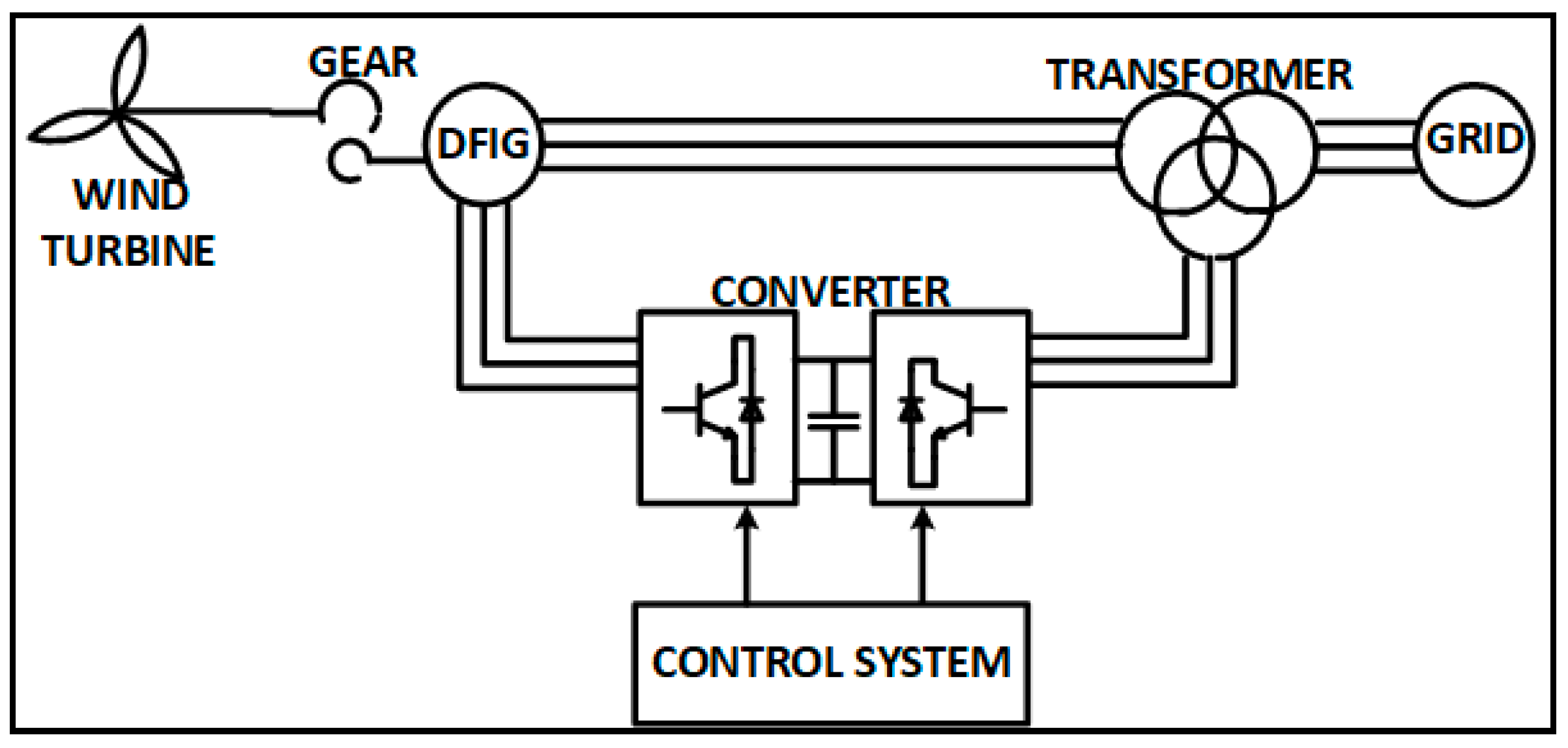
Figure 4.
Control of the machine side converter of the DFIG which includes maximum power point tracking (MPPT), phase locked loop (PLL) and Proportional integral (PI) controllers.
Figure 4.
Control of the machine side converter of the DFIG which includes maximum power point tracking (MPPT), phase locked loop (PLL) and Proportional integral (PI) controllers.
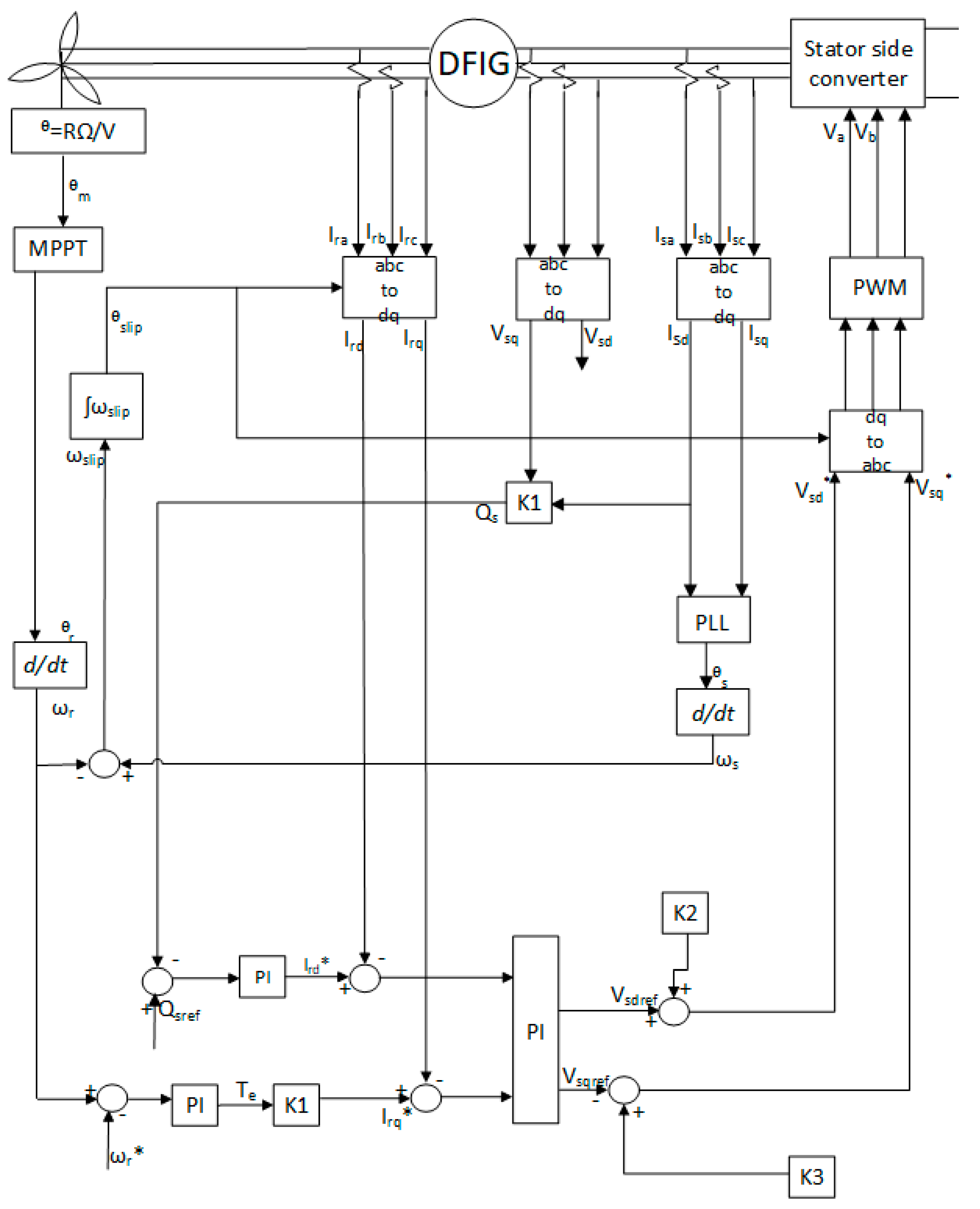
Figure 5.
Control of the grid side converter of the DFIG, including PI controllers, low pass filter, PLL and filter.
Figure 5.
Control of the grid side converter of the DFIG, including PI controllers, low pass filter, PLL and filter.

Figure 6.
Schematic diagram of the PSMG.

Figure 7.
Control of the PMSG, including MPPT, PI controllers, converters, PWM, PLL and filter.
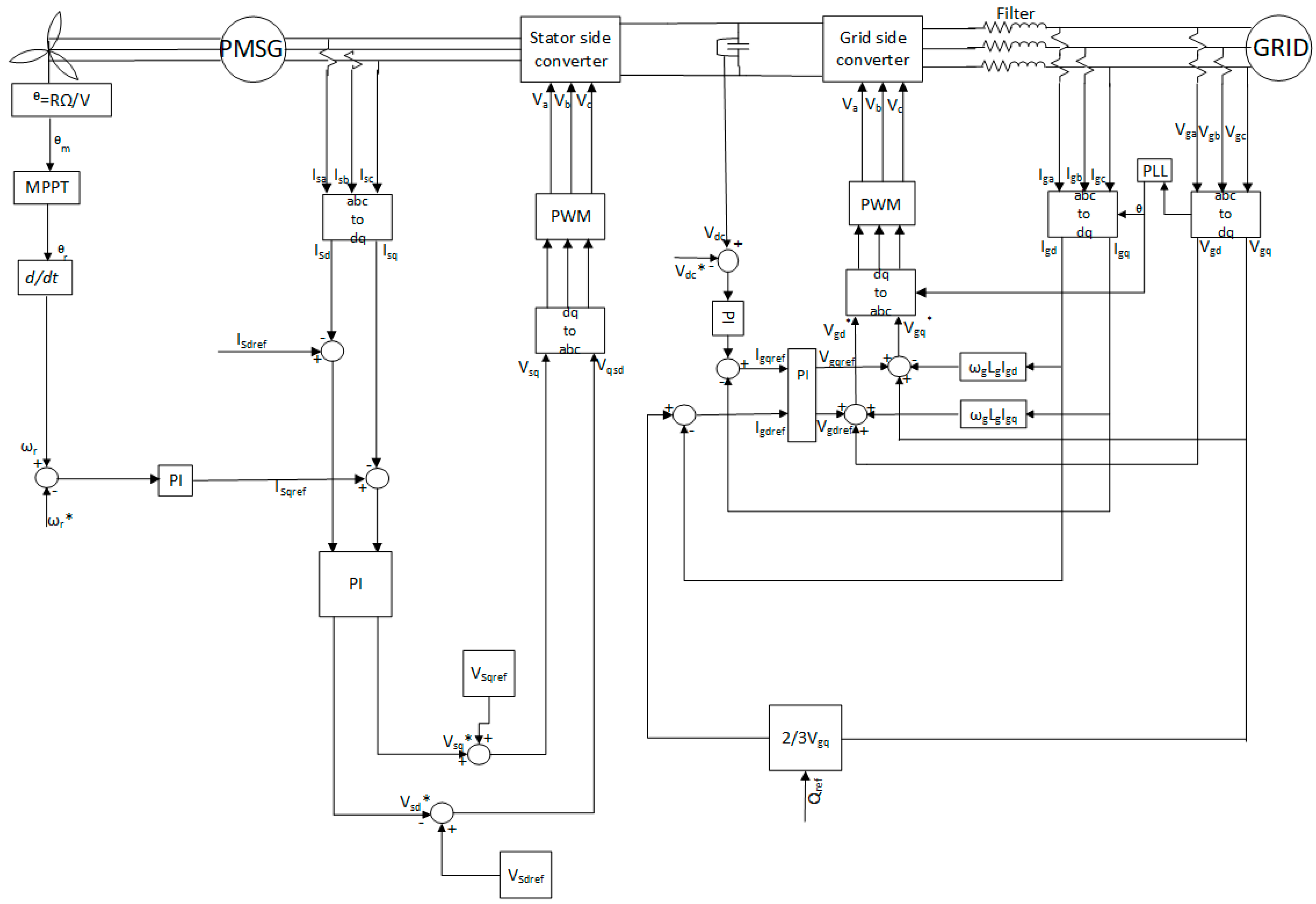
Figure 8.
The ferroresonant results during energization at 0.6 secs on the SCIG wind turbine: (a) Voltage waveform showing overvoltage in phase A and B; (b) Phase plane diagram of phase B depicting chaotic mode.
Figure 8.
The ferroresonant results during energization at 0.6 secs on the SCIG wind turbine: (a) Voltage waveform showing overvoltage in phase A and B; (b) Phase plane diagram of phase B depicting chaotic mode.
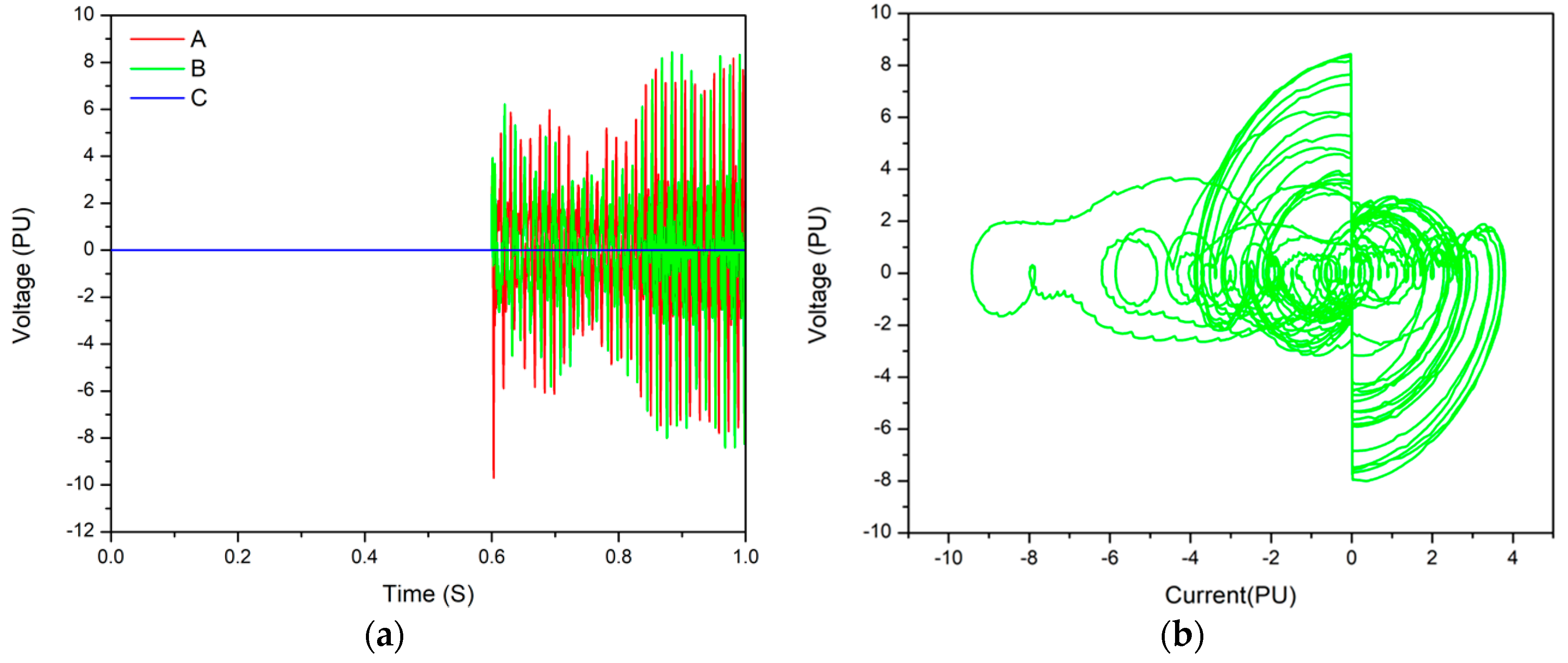
Figure 9.
The ferroresonant results during de-energization at 0.6 secs on the SCIG wind turbine: (a) Voltage waveform of phase A, B and C with highest overvoltage on phase A; (b) Phase plane diagram of phase B having chaos.
Figure 9.
The ferroresonant results during de-energization at 0.6 secs on the SCIG wind turbine: (a) Voltage waveform of phase A, B and C with highest overvoltage on phase A; (b) Phase plane diagram of phase B having chaos.

Figure 10.
The ferroresonant results during energization at 0.6 secs on the WRIG wind turbine: (a) Voltage waveform showing highest overvoltage on phase A; (b) Phase plane diagram of phase B showing chaos.
Figure 10.
The ferroresonant results during energization at 0.6 secs on the WRIG wind turbine: (a) Voltage waveform showing highest overvoltage on phase A; (b) Phase plane diagram of phase B showing chaos.

Figure 11.
The ferroresonant results during de-energization at 0.6 secs on the WRIG wind turbine: (a) Voltage waveform of phase A, B and C with highest overvoltage on phase B; (b) Phase plane diagram of phase B.
Figure 11.
The ferroresonant results during de-energization at 0.6 secs on the WRIG wind turbine: (a) Voltage waveform of phase A, B and C with highest overvoltage on phase B; (b) Phase plane diagram of phase B.
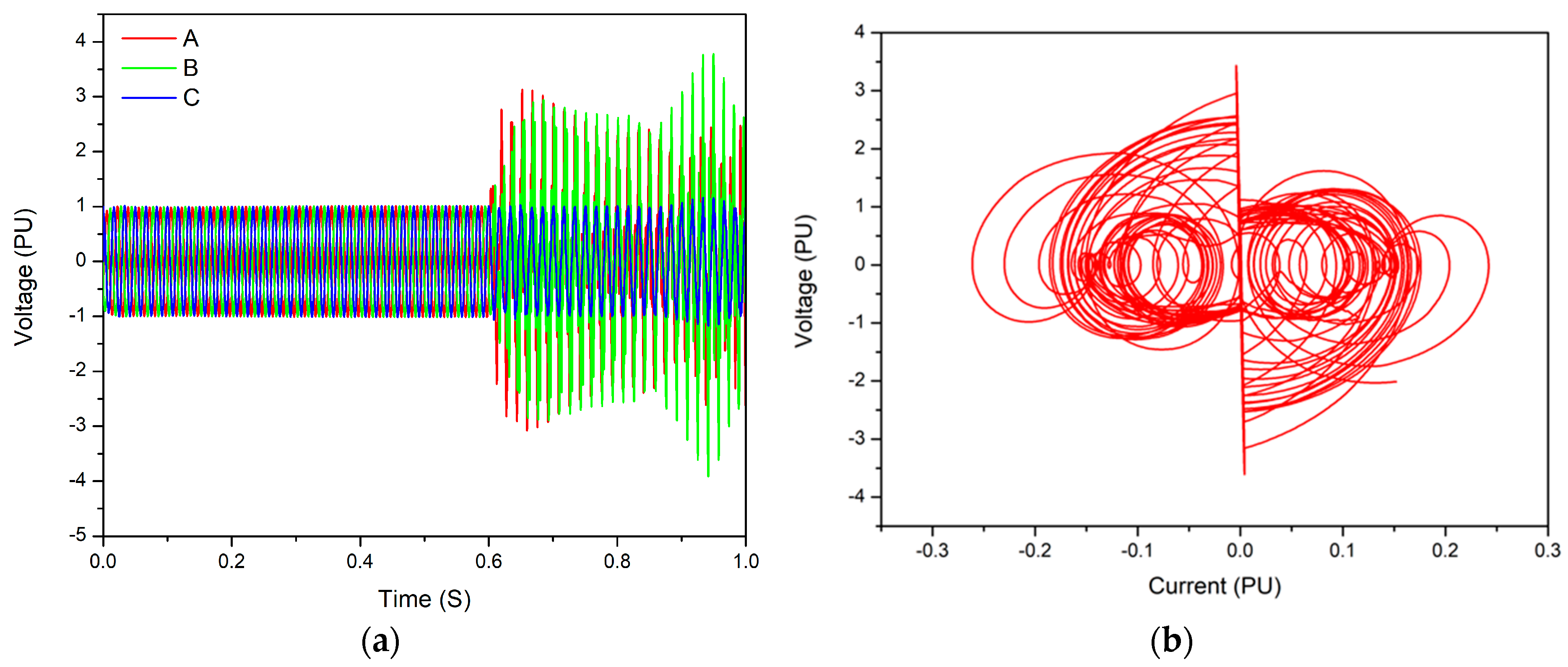
Figure 12.
The ferroresonant results during energization on the DFIG wind turbine: (a) Voltage waveform having highest overvoltage on phase B; (b) Phase plane diagram of phase B depicting quasi-periodic mode.
Figure 12.
The ferroresonant results during energization on the DFIG wind turbine: (a) Voltage waveform having highest overvoltage on phase B; (b) Phase plane diagram of phase B depicting quasi-periodic mode.
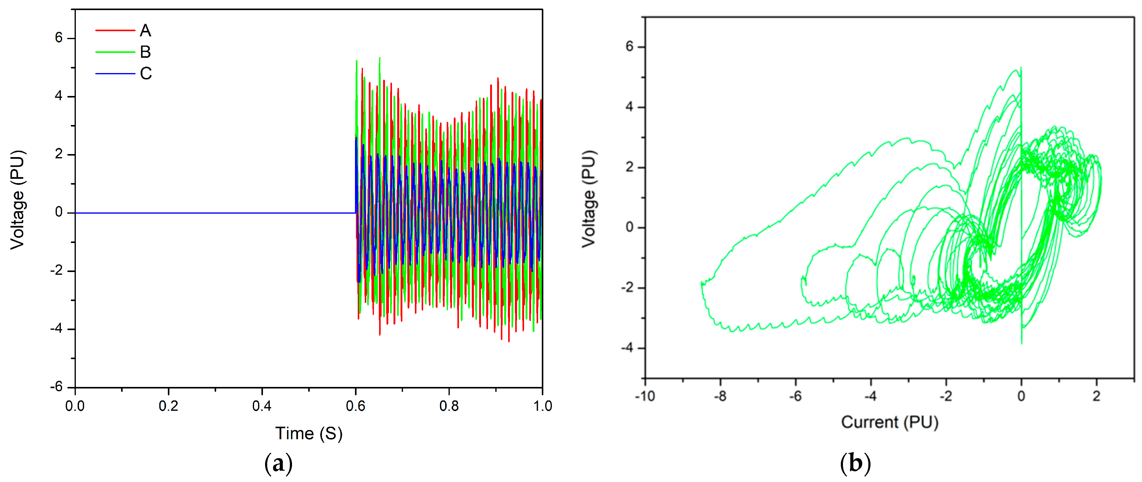
Figure 13.
The ferroresonant results during de-energization at 0.6 secs on the DFIG wind turbine: (a) Voltage waveform, with highest overvoltage on phase B; (b) Phase plane diagram of phase b showing chaotic mode.
Figure 13.
The ferroresonant results during de-energization at 0.6 secs on the DFIG wind turbine: (a) Voltage waveform, with highest overvoltage on phase B; (b) Phase plane diagram of phase b showing chaotic mode.

Figure 14.
The ferroresonant results during energization at 0.6 secs on the PMSG wind turbine: (a) Voltage waveform of phase A, B and C, with phase B having highest overvoltage; (b) Phase plane diagram of phase B showing quasi-periodic ferroresonance.
Figure 14.
The ferroresonant results during energization at 0.6 secs on the PMSG wind turbine: (a) Voltage waveform of phase A, B and C, with phase B having highest overvoltage; (b) Phase plane diagram of phase B showing quasi-periodic ferroresonance.
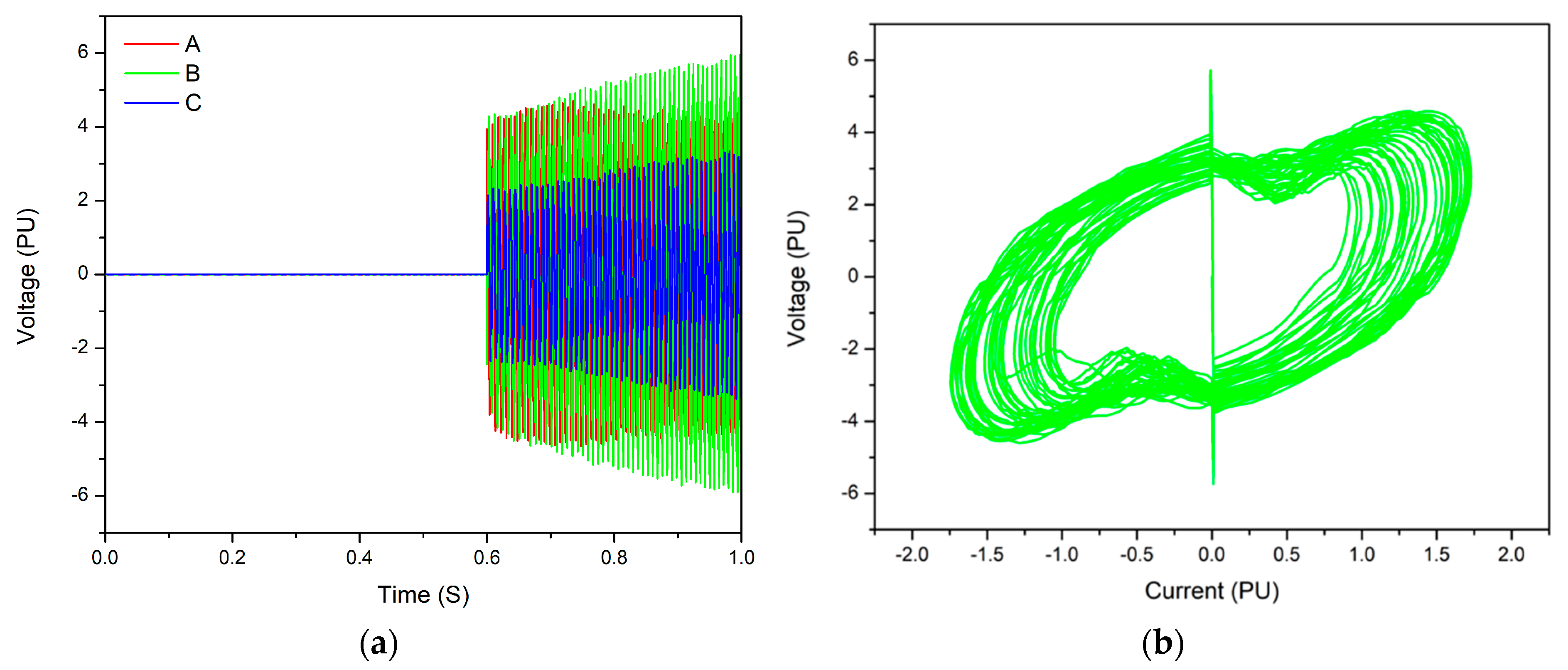
Figure 15.
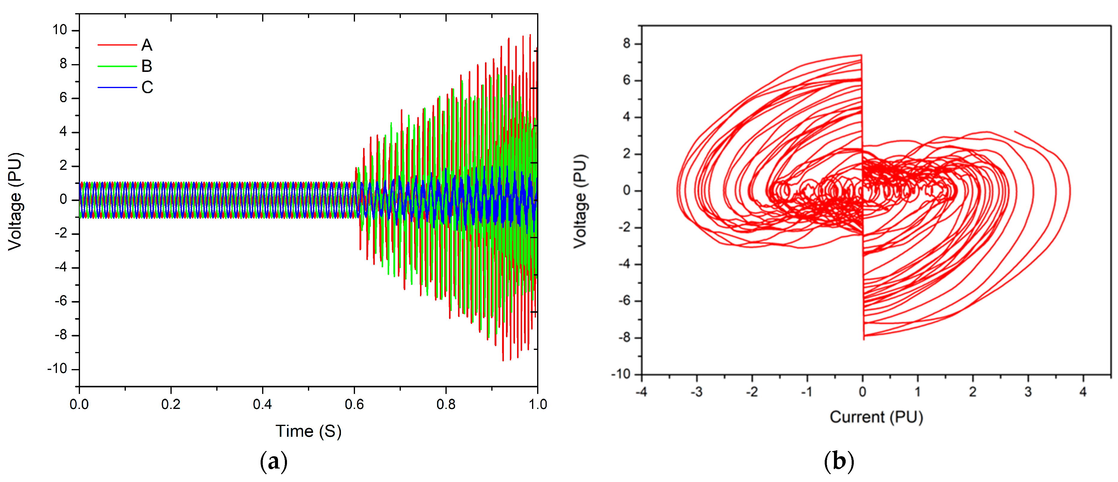
The ferroresonant results during de-energization at 0.6 secs on the PMSG wind turbine: (a) Voltage waveform with highest overvoltage on phase A; (b) Phase plane diagram of phase B showing chaos.
Figure 15.
The ferroresonant results during de-energization at 0.6 secs on the PMSG wind turbine: (a) Voltage waveform with highest overvoltage on phase A; (b) Phase plane diagram of phase B showing chaos.

Table 1.
Squirrel cage induction generator (SCIG) wind turbine data.
| Parameter | Value |
|---|---|
| Rated power | 2 MW |
| Rated frequency | 690 v |
| Rated voltage | 60 Hz |
| Stator resistance Rs | 0.00492 PU |
| Stator inductance Ls | 0.1332 PU |
| Rotor resistance Rr | 0.00445 PU |
| Rotor inductance Lr | 0.1896 PU |
| Mutual inductance | 4.22 PU |
| Number of poles | 4 |
Table 2.
Wound rotor induction generator (WRIG).wind turbine data.
| Parameter | Value |
|---|---|
| Rated power | 2 MW |
| Rated frequency | 690 v |
| Rated voltage | 60 Hz |
| Stator resistance Rs | 0.0071 PU |
| Stator inductance Ls | 0.171 PU |
| Rotor resistance Rr | 0.005 PU |
| Rotor inductance Lr | 0.156 PU |
| Mutual inductance | 2.9 PU |
| Number of poles | 4 |
Table 3.
Doubly fed induction generators (DFIG) wind turbine data.
| Parameter | Value |
|---|---|
| Rated power | 2 MW |
| Rated frequency | 690 v |
| Rated voltage | 60 Hz |
| Stator resistance Rs | 0.034 PU |
| Stator inductance Ls | 0.17 PU |
| Rotor resistance Rr | 0.018 PU |
| Rotor inductance Lr | 0.17 PU |
| Mutual inductance | 3.2 PU |
| Number of poles | 4 |
Table 4.
PMSG wind turbine data.
| Parameter | Value |
|---|---|
| Rated power | 2 MW |
| Rated frequency | 690 v |
| Rated voltage | 9.25 Hz |
| Stator resistance | 0.008 PU |
| Stator inductance (d, q axis) | 0.167 PU |
| Permanent magnet flux | 0.19 PU |
| Number of poles | 24 |
Table 5.
Wind turbine transformer data.
| Parameters | Primary | Secondary | |
|---|---|---|---|
| Wind turbine Transformer (2.5 MVA) | Vector group | D | Yn11 |
| Voltage (kV) | 0.69 | 33 | |
| R (PU) | 0.00025 | 0.042 | |
| L (PU) | 0.03 | 0.314 |
Table 6.
Positive magnetization data of the transformer.
| Current (PU) | Flux (PU) |
|---|---|
| 0 | 0 |
| 0.102 | 1.12 |
| 1.0 | 1.42 |
Table 7.
Ferroresonant overvoltage during nuisance operations of the circuit breaker for different wind turbine configurations.
Table 7.
Ferroresonant overvoltage during nuisance operations of the circuit breaker for different wind turbine configurations.
| Wind Turbine Generator Type | Switching Operation | Ferroresonant Overvoltage (PU) | Ferroresonance Mode |
|---|---|---|---|
| SCIG | Energization | 10.1 | Chaotic |
| De-energization | 5.71 | Chaotic | |
| WRIG | Energization | 8.22 | Chaotic |
| De-energization | 4.01 | Chaotic | |
| DFIG | Energization | 5.08 | Quasi-periodic |
| De-energization | 4.43 | Chaotic | |
| PMSG | Energization | 6.12 | Quasi-periodic |
| De-energization | 9.58 | Chaotic |
© 2019 by the authors. Licensee MDPI, Basel, Switzerland. This article is an open access article distributed under the terms and conditions of the Creative Commons Attribution (CC BY) license (http://creativecommons.org/licenses/by/4.0/).
Share and Cite
MDPI and ACS Style
Akinrinde, A.; Swanson, A.; Tiako, R. Dynamic Behavior of Wind Turbine Generator Configurations during Ferroresonant Conditions. Energies 2019, 12, 639. https://doi.org/10.3390/en12040639
AMA Style
Akinrinde A, Swanson A, Tiako R. Dynamic Behavior of Wind Turbine Generator Configurations during Ferroresonant Conditions. Energies. 2019; 12(4):639. https://doi.org/10.3390/en12040639
Chicago/Turabian StyleAkinrinde, Ajibola, Andrew Swanson, and Remy Tiako. 2019. "Dynamic Behavior of Wind Turbine Generator Configurations during Ferroresonant Conditions" Energies 12, no. 4: 639. https://doi.org/10.3390/en12040639
Note that from the first issue of 2016, this journal uses article numbers instead of page numbers. See further details here.