Effect of Tailing-Edge Thickness on Aerodynamic Noise for Wind Turbine Airfoil

Abstract

The influence of wind turbine airfoil trailing edge thickness on aerodynamics and aerodynamic noise characteristics was studied using the computational fluid dynamics (CFD)/ Ffowcs Williams–Hawkings (FW–H) method in the present work. First, the airfoil of a DU97-W-300-flatback airfoil was chosen as the research object, and numerical method validation was performed. Three kinds of turbulence calculation methods (unsteady Reynolds average Navier-Stokes (URANS), detached eddy simulation (DES), and large eddy simulation (LES)) were investigated in detail, and three sets of grid scales were used to study the impact of the airfoil on the aerodynamic noise. Secondly, the airfoil trailing edge thickness was changed, and the impact of trailing edge thickness on aerodynamics and aerodynamic noise was investigated. Results show that three kinds of turbulence calculation methods yield the same sound pressure frequency, and the magnitude of the sound pressure level (SPL) corresponding to the mean frequency is almost the same. The calculation of the SPL of the peak value and the experimental results can match well with each other, but the calculated core frequency is slightly lower than the experimental frequency. The results of URANS and DES are closer to each other with a changing trend of SPL, and the consequences of the DES calculation are closer to the experimental results. From the comparison of two airfoils, the blunt trailing edge (BTE) airfoil has higher lift and drag coefficients than the original airfoil. The basic frequency of lift coefficients of the BTE airfoil is less than that of the original airfoil. It is demonstrated that the trailing vortex shedding frequency of the original airfoil is higher than that of the BTE airfoil. At a small angle of attack (AOA), the distribution of SPL for the original airfoil exhibits low frequency characteristics, while, at high AOA, the wide frequency characteristic is presented. For the BTE airfoil, the distribution of SPL exhibits low frequency characteristics for the range of the AOA. The maximum AOA of SPL is 4° and the minimum AOA of SPL is 15°, while, for the original airfoil, the maximum AOA of SPL is 19°, and the minimum AOA is 8°. For most AOAs, the SPL of the BTE airfoil is larger than that of the original airfoil.

1. Introduction

With the developments in wind energy, there are increasingly more large-scale wind farms being built close to the residential areas [1,2,3]. This poses a problem as the noise generated from the wind turbines has a negative effect on the health and quality of life of the affected residents [4,5,6,7]. As such, many researchers have recently taken an interest in the topic [8,9,10,11]. Wind turbine noise mainly consists of mechanical and aerodynamic noise. Mechanical noise is mainly caused by the irregular vibration of friction and the unbalanced forces between rotating parts of a machine. The mechanical noise can be improved by increasing the mechanical manufacturing accuracy, improving lubrication and reducing friction. On the other hand, aerodynamic noise can be caused by the interaction between the blade and the tower, as well as the effect of fluid on the blade [12]. Therefore, aerodynamic noise has become an important factor in noise control of wind turbines [13].

With the large-scale development of wind turbines, the blunt trailing edge (BTE) airfoil is widely applied in wind turbine blades for its better structural and aerodynamic characteristics [14,15,16]. However, the BTE airfoil possesses some significant disadvantages, such as poor drag performance, as well as large noise generation from vibrations. Many studies have been carried out on trailing edge noise in recent years [17]. The trailing edge noise was firstly experimentally studied in 1973 by united aircraft research laboratories and the Sikorsky aircraft company [18]. The test airfoils were NACA0012 and NACA0018, and the wind tunnel experiment Reynolds number was 8 × 10⁵–2.2 × 10⁶. The results show that for the same attack at low Reynolds numbers, the trailing edge noise data can be detected, whereas, at high Reynolds numbers, trailing edge noise is difficult to detect accurately. Brooks et al. [19] performed an investigation on the NACA0012 airfoil at NASA Langley Research Center using quiet flow facility (QFF) acoustic equipment. A series of pressure sensors were installed on the airfoil surface to monitor the pressure fluctuation of the airfoil surface, and the correlation between the trailing edge noise and the trailing edge thickness was analyzed by varying the thickness value. They also adopted the coherent output power (COP) method to study the airfoil-self noise comprehensively, by changing the angle of attack (AOA), chord length, and incoming flow and tip conditions.

To calculate aerodynamic noise of airfoils, Lighthill [20] derived the famous Lighthill equation from the basic theory of aerodynamic acoustics. In his research, the method of using a point source to describe the hydrodynamic sound source was proposed. The sound field and acoustic analogy theory of hydrodynamic sound source were solved using classical acoustics. Although the Lighthill equation considered the quadrupole source in turbulent flow, the effect of solid boundaries in the fluid on the sound field is not included. In 1955, the Lighthill equation was extended by Curle [21] using the Kirchhoff integral method, and the Curle equation was proposed. In 1969, Ffowcs Williams and Hawkings [22] derived the FW–H acoustic wave equation, which is suitable for solving the noise problem of moving parts. In 1997, Francescantonio [23] proposed a new prediction method for aerodynamic noise, named the K–FW–H method.

In 1999, Singer et al. [24] numerically investigated the airfoil trailing edge noise of NACA airfoil using the computational fluid dynamics (CFD)/Ffowcs Williams–Hawkings (FW–H) method. Results show that the trailing edge vortex can be induced by the interaction between the wing boundary layer and the airfoil trailing edge. In addition, it is the main reason for aerodynamic noise. In 2003, Ewert et al. [25] solved the tailing edge noise of a wind turbine using large eddy simulation (LES) and the acoustic perturbation equation (APE). In the same project, the modified boundary-scale method was first adopted to compute the turbulent boundary layer. Then, LES was used to simulate the flow field at the trailing edge of the wind turbine. Finally, the flow field information was used to solve the initial values of the linear APE equation. In 2004, Shen et al. [26] proposed a numerical algorithm to simulate the process of the acoustic noise generation based on the collocated grids. The new method was used to simulate the flow around a circular cylinder and a NACA0015 airfoil. The results show that a viscous–viscous coupling is more natural and gives excellent results. In 2010, Sandberg et al. [27] studied the NACA0012 airfoil by direct numerical simulation (DNS). The results indicate that the source position of the airfoil surface can be determined by the correlation of acoustics and hydrodynamics. At low Reynolds numbers, the trailing edge noise produced by the transition of fluid from boundary layer to turbulence is greater than that without transition. The analysis also shows that trailing edge noise is the main source for low-frequency noise.

Ikeda et al. [28] adopted the direct noise simulation method to simulate the noise produced by the NACA0012 and NACA0006 airfoils, and the effect of chord length on trailing edge noise was investigated. Albarracin et al. [29] used the URANS method to calculate the aerodynamic noise for an airfoil with a sharp trailing edge, and the results were compared with experimental data. Lummer et al. [30] investigated the aerodynamic noise characteristics of a symmetrical Joukowsky airfoil at a 0° AOA. In addition, the influence of the trailing edge vortex on aerodynamic noise was also analyzed. Jones et al. [31] also calculated the aerodynamic noise of an NACA0012 airfoil using the computational aero-acoustics (CAA)method. The airfoil self-noise characteristics were studied at four AOAs. The results show that at a small AOA, the airfoil noise value is higher than that at a large AOA. In addition, the aerodynamic noise of an airfoil is closely related to the shear effect of the trailing vortex.

Shin et al. [32] adopted the LES method to numerically study the noise of turbine machinery with BTE blades. The trailing edge flow field and noise characteristics were analyzed. Fleig et al. [33] also used the LES method to investigate the wind turbine blade tip vortex noise. Fleig and Lida et al. [34] studied the tip vortex noise of rotating wind turbine blades. Marsden et al. [35] used LES to study and compare the difference in surface boundary layer transition of the flow over airfoils in two and three dimensions. Results show that the method can accurately predict the position of boundary layer transition, as well as the aerodynamic noise. Jiang and Li et al. [36,37] used the computation aeroacoustics (CAA) method to simulate the airfoil self-noise at different noise characteristics. Takagi et al. [38] and Nakano [39] studied the cylindrical/airfoil interference noise and airfoil self-noise characteristics. Subsequently, they analyzed the flow field and aerodynamic noise characteristics of an airfoil with a cylindrical spoiler. Results show that the interference noise produced by a cylindrical spoiler is higher than that of an airfoil without the spoiler. Further, it was concluded that the boundary layer transition is the main reason for noise generation. Jacob et al. [40] and Bjorn et al. [41] studied the aerodynamic noise characteristics of a cylinder and a NACA0012 airfoil, as well as the interactions between them. The results indicate that when using the detached eddy simulation (DES) method with the FW–H equation, it can better obtain the acoustic signals of a complex flow field. Moreover, Giret [42] also researched the unsteady interference flow field of a cylinder/airfoil. The results show that the chord length and column–airfoil arrangement have a stronger effect on noise generation.

Overall, the trailing edge noise accounts for the majority of the aerodynamic noise of airfoil. Thus, it is very important to study the influence of trailing edge thickness on aerodynamic noise for thick airfoils. At present, few studies referring to the influence of trailing edge thickness on airfoil aerodynamic noise have been published. In this study, the DU97-W-300-flatback (BTE) airfoil is chosen as the research object, and the effects of three different turbulence models (URANS, DES, LES) are studied. Then, the characteristics of the BTE airfoil and the original DU97-W-300 airfoil are investigated, and the influence of trailing edge thickness on airfoil aerodynamic noise at different AOAs are analyzed.

2. Methodology

2.1. Numerical Conditions

2.1.1. Large Eddy Simulation

According to the vorticity theory of turbulence, the turbulent flow is composed of multi-scale vortices. Larger scale vortices cause turbulent fluctuation and fluid mixing. The main characteristics are obtaining energy from the mainstream flow, and playing an important role in the turbulent diffusion of energy and the generation of turbulent energy in turbulent flow. Small-scale vortices obtain energy from the interaction of large-scale vortices, and small-scale vortices mainly play the role of energy dissipation. After filtering the Navier-Stokes (N-S)equation with a filter function, the governing equation of the large eddy simulation (LES) method [43] in incompressible flow can be obtained:

$$\frac{\partial \rho }{\partial t}+\frac{\partial \rho u_i}{\partial x_i}=0$$

(1)

$$\frac{\partial \left(\rho \overline{u_i}\right)}{\partial t}+\frac{\partial \left(\rho \overline{u_i}\overline{u_j}\right)}{\partial x_j}=\frac{\partial }{\partial x_j}\left(\mu \frac{\partial \overline{{\sigma }_{ij}}}{\partial x_j}\right)-\frac{\partial \overline{p}}{\partial x_i}-\frac{\partial {\tau }_{ij}}{\partial x_j}$$

(2)

where ${\sigma }_{ij}$ is stress tensor and ${\tau }_{ij}$ is subgrid stress.

For the subgrid model, the Smagorinsky–Lilly model is used to solve the problem in this paper. This model was first proposed by Smagorinsky. The eddy viscosity is defined as follows:

$${\mu }_t=\rho L_s{}^2\left|\overline{s}\right|$$

(3)

where $L_s$ is the mixed length of the grid and $\overline{s}\equiv \sqrt{2\overline{s_{ij}}\overline{s_{ij}}}$.

In the Fluent software, $L_s=\min (\mathrm{kd},{\mathrm{C}}_s{\mathrm{V}}^{1/3})$, where k is a constant, d is the nearest distance from the wall, ${\mathrm{C}}_s$ is the Smagorinsky constant (in this paper, the value of ${\mathrm{C}}_s$ is 0.1), and V is the volume of the calculation unit.

2.1.2. Transitional Shear Stress Transport (SST)

The transitional SST model is a four-equation model, which is the same as SST model [44]. The k-ω model is used in the near-wall region and the k-ε model is used in the free-flow region. The k-ω SST model is obtained. On this basis, the transport equation of intermittent factor γ and the Reynolds number $R{\overline{e}}_{\theta t}$ equation of local transition momentum thickness are introduced to form the four-equation model [45]. Transition prediction includes predicting the starting position of transition and predicting the length of the transition region, for which $R{\overline{e}}_{\theta t}$ constitutes a criterion for predicting the starting position of transition and γ is used to simulate the transition region.

The $R{\overline{e}}_{\theta t}$ transport equation is as follows:

$$\frac{\partial (\rho R{\overline{e}}_{\theta t})}{\partial t}+\frac{\partial (\rho U_{j}R{\overline{e}}_{\theta t})}{\partial x_j}=P_{\theta t}+\frac{\partial }{\partial x_j}\left[{\sigma }_{{}_{\theta t}}(\mu +{\mu }_t)\frac{R{\overline{e}}_{\theta t}}{\partial x_j}\right]$$

(4)

in which:

$$P_{\theta t}=c_{\theta t}\frac{\rho }{t}(R{e}_{\theta t}-R{\tilde{e}}_{\theta t})(1.0-F_{{}_{\theta t}})$$

(5)

and:

$$F_{{}_{\theta t}}=\min \left[\max \left[F_{wake}{e}^{{\left(-\frac{y}{\delta }\right)}^4},1.0-{\left[\frac{\gamma -\raisebox{1ex}{$1$}\!\left/ \!\raisebox{-1ex}{$50$}\right.}{1.0-\raisebox{1ex}{$1$}\!\left/ \!\raisebox{-1ex}{$50$}\right.}\right]}^2\right],1.0\right], t=c_{\theta t}\frac{500\mu }{\rho U^2}, {\theta }_{BL}=\frac{R{\overline{e}}_{\theta t}\mu }{\rho U}, {\delta }_{BL}=\frac{15}{2}{\theta }_{BL}, \delta =\frac{50\Omega y}{U}{\delta }_{BL}, R{e}_{\omega }=\frac{\rho \omega y^2}{\mu }, F_{wake}=e^{-{\left(\frac{R{e}_{\omega }}{1E+5}\right)}^2}$$

where P_θt ensures that $R{\tilde{e}}_{\theta t}=R{e}_{\theta t}$ on outside of boundary layer; F_θt is a switching function equal to 0 outside the boundary layer and 1 inside the boundary layer; F_wake ensures that F_θt is 0 in the downstream area of the surface; and constant terms are: c_θt = 0.03, σ_θt = 2.0.

$R{\overline{e}}_{\theta t}$ is zero flux at the wall, and the value of $R{\overline{e}}_{\theta t}$ at the inlet is modified according to the turbulence intensity. The model consists of three empirical relationships. Re_θt is the local transition Reynolds number, which is based on the empirical relationship obtained from experiments, and is a function of turbulence and local pressure gradient; F_length is used to adjust the length of the transition region, which is a function of the local Reynolds number $R{\overline{e}}_{\theta t}$.

$$R{e}_{\theta t}=f(Tu,{\lambda }_{\theta })$$

(6)

$$F_{length}=f(R{\tilde{e}}_{\theta t})$$

(7)

$$R{e}_{\theta c}=f(R{\tilde{e}}_{\theta t})$$

(8)

Turbulence Tu is based on empirical relations:

$$Tu=\frac{100}{U}\sqrt{\frac{2}{3}k}$$

(9)

Pressure gradient is defined as:

$${\lambda }_{\theta }=\left(\frac{{\theta }^2}{\nu }\right)\frac{dU}{ds}$$

(10)

where dU/ds is the flow acceleration.

The γ transport equation is written:

$$\frac{\partial (\rho \gamma )}{\partial t}+\frac{\partial (\rho U_j\gamma )}{\partial x_j}=P_{\gamma 1}-E_{\gamma 1}+P_{\gamma 2}-E_{\gamma 2}+\frac{\partial }{\partial x_j}\left[\left(\mu +\frac{{\mu }_t}{{\sigma }_{\gamma }}\right)\frac{\partial \gamma }{\partial x_j}\right]$$

(11)

$$P_{\gamma 1}=C_{a1}{F}_{length}\rho S{\left[\gamma F_{oneset}\right]}^{C_{\gamma 3}}$$

(12)

$$E_{\gamma 1}=C_{e1}{P}_{\gamma 1}\gamma$$

(13)

where S is the strain rate, F_length is used to adjust the length of the transition zone. The formulae for fracture and re-lamination are as follows:

$$P_{\gamma 2}=C_{a2}\rho \Omega \gamma F_{turb}$$

(14)

$$E_{\gamma 2}=C_{e2}{P}_{\gamma 2}\gamma$$

(15)

where Ω is the size of vorticity, and the beginning of transition is controlled by the following formulae:

$$R{e}_V=\frac{\rho y^{2}S}{\mu }$$

(16)

$$R_T=\frac{\rho k}{\mu \omega }$$

(17)

$$F_{oneset1}=\frac{R{e}_V}{2.193R{e}_{\theta c}}$$

(18)

$$F_{oneset2}=\min \left[\max \left(F_{oneset1},F_{oneset1}^4\right),2.0\right]$$

(19)

$$F_{oneset3}=\max \left(1-{\left(\frac{R_T}{2.5}\right)}^3,0\right)$$

(20)

$$F_{oneset}=\max \left(F_{oneset2}-F_{oneset3},0\right)$$

(21)

$$F_{turb}=e^{-{\left(\frac{R_T}{4}\right)}^4}$$

(22)

where ρ is fluid density; t is physical time; U_j is velocity; x_j is a coordinate; k is turbulent kinetic energy; ω is specific dissipation rate of turbulent kinetic energy; k and ω are provided by the SST model; μ is molecular dynamic viscosity; R_T is the viscous ratio; Re_V is vorticity Reynolds number; y is wall distance; Re_θc is critical Reynolds number for the increase of the intermittence factor in the boundary layer; and constant terms are: C_a1 = 2.0, C_e1 = 1.0, C_a2 = 0.06, C_e2 = 50, c_γ3 = 0.5, σ_γ = 1.0.

When there is separation transition in the flow field, γ will increase rapidly at the separation bubble position. With the increase of the turbulent viscous ratio, the increasing trend of γ tends to be gentle. Therefore, when separation-induced transition exists in the flow field, the intermittent factor γ_sep can be expressed as follows:

$${\gamma }_{sep}=\min \left[C_{s1}\max \left(\left(\frac{R{e}_V}{3.235R{e}_{\theta c}}\right)-1,0\right)F_{reattach},2\right]F_{\theta t}$$

(23)

$$F_{reattach}=e^{-{\left(\frac{R_T}{20}\right)}^4}$$

(24)

where F_reattach is such that when the turbulent viscosity is larger than R_T, γ_sep tends to zero, so the effective intermittent factor is expressed as follows:

$${\gamma }_{eff}=\max \left(\gamma ,{\gamma }_{sep}\right)$$

(25)

The transition model controls the generation and dissipation terms of the turbulent kinetic energy equation in the SST model by means of an intermittent factor.

The modified k equation can be written:

$$\frac{\partial }{\partial t}(\rho k)+\frac{\partial }{\partial x_i}(\rho k{u}_i)=\frac{\partial }{\partial x_j}({\Gamma }_k\frac{\partial k}{\partial x_j})+G_k^{\ast }-Y_k^{\ast }+S_k$$

(26)

$$G_k^{\ast }={\gamma }_{eff}{\tilde{G}}_k$$

(27)

$$Y_k^{\ast }=\min \left(\max \left({\gamma }_{eff},0.1\right),1.0\right)Y_k$$

(28)

The ω equation can be written:

$$\frac{\partial }{\partial t}(\rho \omega )+\frac{\partial }{\partial x_j}(\rho \omega u_i)=\frac{\partial }{\partial x_j}\left[\left(\mu +\frac{{\mu }_t}{{\sigma }_{\omega }}\right)\frac{\partial \omega }{\partial x_j}\right]+\alpha \frac{\omega }{k}{P}_k-\beta \rho {\omega }^2+P_{\omega b}$$

(29)

2.1.3. Detached Eddy Simulation

The detached eddy simulation (DES) method is a hybrid simulation method of Reynolds average Navier-Stokes (RANS)/ large eddy simulation (LES). It is a simulation method that combines the advantages of LES and RANS and was proposed by Spalart in 1997 [46]. This method is simulated by the RANS method in the near-wall area and the LES method in the main flow area far from the wall. In this way, not only can the number of meshes on the wall be greatly reduced, but also the details of the flow field can be obtained by using large eddy simulation in the mainstream region, thereby taking into account the respective advantages of RANS and LES.

The basic form of DES is as follows:

$$\frac{D\tilde{v}}{Dt}=c_{b1}\tilde{S}\tilde{v}+\frac{1}{\sigma }[\nabla •((v+\tilde{v})\nabla \tilde{v})+c_{b2}{(\nabla \tilde{v})}^2]-c_{w1}{f}_w{\left[\frac{\tilde{v}}{d}\right]}^2$$

(30)

where d is the length scale, and the relationship between variable $\tilde{v}$ and turbulent viscous $v_{\mathrm{t}}$ is given by the following formula:

$$v_t=\tilde{v}{f}_{v1}$$

(31)

$$f_{v1}=\frac{{\chi }^3}{{\chi }^3+c_{v1}^3}$$

(32)

$$\chi \equiv \frac{\tilde{v}}{v}$$

(33)

where $v$ is fluid viscous and the generating term $\tilde{S}$ is:

$$\tilde{S}\equiv f_{v3}S+\frac{\tilde{v}}{{\kappa }^2{d}_w^2}{f}_{v2}$$

(34)

where:

$$f_{v2}={\left[1+\frac{\chi }{c_{v2}}\right]}^{-3}, f_{v3}=\frac{(1+\chi f_{v1})(1-f_{v2})}{\chi }, f_w=g\left[\frac{1+c_{w3}^6}{g^6+c_{w3}^6}\right], g=r+c_{w2}(r^6-r), r\equiv \frac{\tilde{v}}{\tilde{S}{\kappa }^2{d}_w^2}$$

The value of the constant terms are:

$$\kappa =0.41,\sigma =2/3,c_{b1}=0.1355,c_{b2}=0.622,c_{w1}\equiv \frac{c_{b1}}{{\kappa }^2}+\frac{1+c_{b2}}{\sigma },c_{w2}=0.3,c_{w3}=2,c_{v1}=7.1$$

In order to implement the RANS method in the near-wall area, the LES method is adopted in the main stream area, and the length scale in the formula is replaced by:

$$\tilde{d}=\min (d_w,{\mathrm{C}}_{DES}\Delta )$$

(35)

where $\Delta =\max (\Delta x,\Delta y,\Delta z)$ and Δ takes the maximum grid values of x, y and z directions in the flow field; $C_{DES}=0.65$; $d_w$ represents the distance from the center of the grid to the wall. In this way, the RANS method is used in $d_w<{\mathrm{C}}_{DES}\Delta$ regions and the LES method is used in $d_w>{\mathrm{C}}_{DES}\Delta$ regions.

2.1.4. Mesh Setup

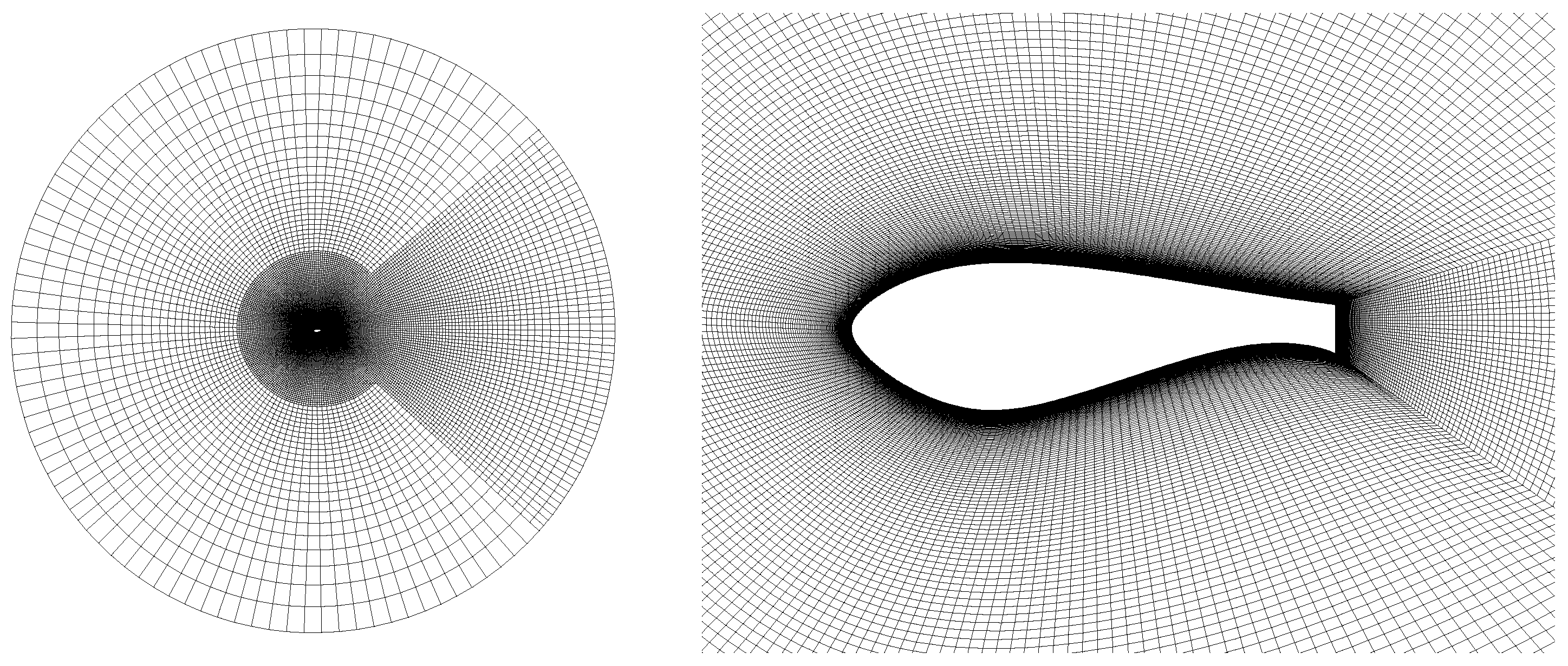
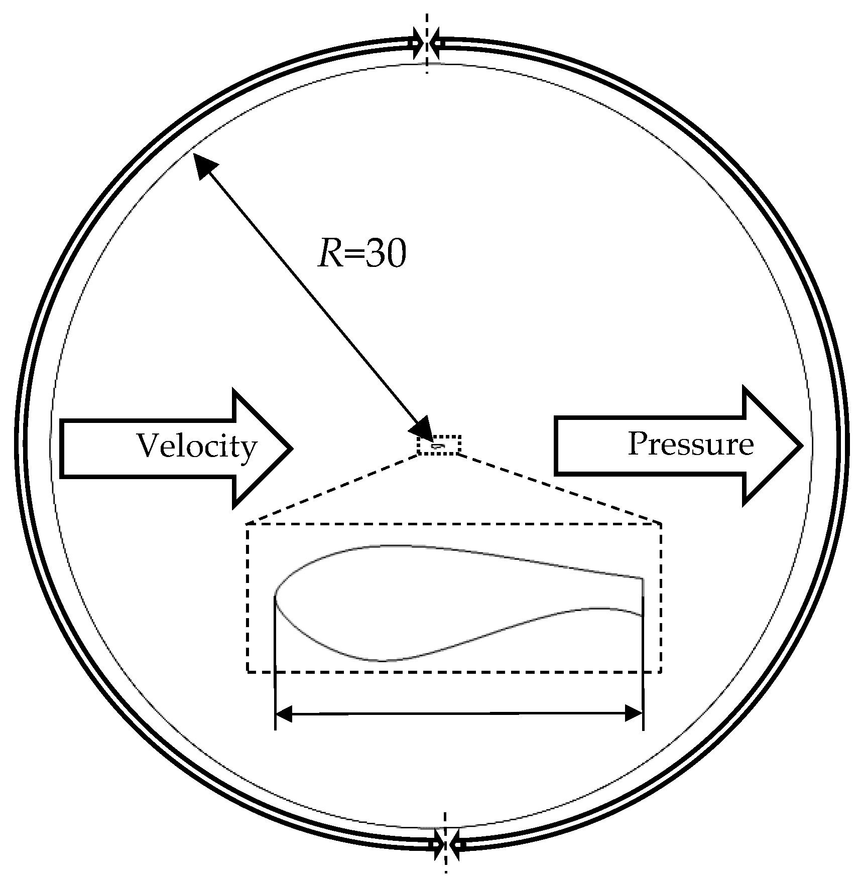
ICEM software was used to generate the mesh. The computational domain was round, and the radius was 30C (C is chord length of airfoil). In the near-flow field of the airfoil, the pressure gradient was large, and more mesh was needed to obtain more detailed flow field information, while in the far-flow field of the airfoil, the pressure gradient was small, and the mesh density was relatively small according to the physical information. The trailing edge of the airfoil shed vortices and separating vortices moved downstream along the inflow direction, so more meshes were needed along the downstream vortex of the trailing edge. Thus, mesh refinement was performed in the region close to the airfoil, up to a distance of 10C away from the airfoil and, downstream of the airfoil, mesh encryption was preformed, as show in Figure 1. The mesh height along the first layer of the wall was 0.01 mm, the y+ value was less than 1, and the wall normal expansion ratio in the boundary layer was 1.05, which met the requirements for turbulent calculation. Structural mesh was used in the flow field. Three sets of mesh (Mesh 1, Mesh 2 and Mesh 3) were divided. The distribution of mesh is shown in

Table 1. Mesh distribution.

Mesh	Number of Circumferential	Number of Radial Directions	Number of Mesh Elements
Mesh 1	240	330	70,000
Mesh 2	340	460	140,000
Mesh 3	480	640	280,000

. The overall quality of mesh in the ICEM software was more than 0.7. The front side of the circle was set as the velocity inlet, and the back side was set as the pressure outlet. The no-slip boundary was chosen on the airfoil surface. Computational domain size and boundary condition settings are shown in Figure 2. The Reynolds number based on chord length was 3 × 10⁶, and the free stream velocity was 43.8 m/s.

2.2. Acoustic Analogy

Noise prediction was performed using the Ffowcs Williams–Hawkings (FW-H) equation [20]. This model calculates the far-field noise that is radiated from the near-field data of the computational fluid dynamics (CFD) result.

Two basic equations had been provided by Lighthill: the continuity equation of fluid mass conservation in the volume element (Scalar equation), and the particle motion equation obtained by the fluid volume element. It should be noted that the formulae can only be established in incompressible fluids.

$$\frac{\partial \rho }{\partial t}+\frac{\partial \rho u_j}{\partial x_j}=0$$

(36)

$$\rho \frac{\partial u_i}{\partial t}+\rho u_j\frac{\partial u_i}{\partial x_j}=-\frac{\partial p_{ij}}{\partial x_j}$$

(37)

Equation (36) multiplied by $u_i$ is transformed into the component description of the vector equation, and, when added to Equation (37), the momentum equation can be obtained:

$$\frac{\partial (\rho u_i)}{\partial t}+\frac{\partial \rho u_i{u}_j}{\partial x_j}=-\frac{\partial p_{ij}}{\partial x_j}$$

(38)

The Heaviside generalized function is written:

$$H(f)=\{\begin{array}{l}1,f(x,t)>0\\ 0,f(x,t)<0\end{array}$$

(39)

where $f(x,t)=0$ is the governing surface equation.

The Heaviside flow parameters of the generalized function are as follows:

$$\{\begin{array}{l}\overline{\rho }={\rho }^{\prime }H(f)+{\rho }_0\\ \overline{u_i}=u_{i}H(f)\\ \overline{p_{ij}}=p_{ij}H(f)-{\mathrm{p}}_0{\delta }_{ij}\end{array}$$

(40)

where $\rho$, $u_i$, and $p_{ij}$ denote fluid density, particle velocity and stress tensor, respectively. The lower corner sign 0 denotes the undisturbed quantity, the apostrophe denotes the disturbed quantity, and ${\delta }_{ij}$ denotes the Crohneck symbol.

The generalized continuity equation and momentum equation are obtained by introducing generalized flow parameters into the continuity equation and momentum equation:

$$\frac{\partial }{\partial t}[{\rho }^{\prime }H(f)]+\frac{\partial }{\partial x_i}[\rho u_{i}H(f)]={\rho }_0{u}_i\frac{\partial H}{\partial x_i}$$

(41)

$$\frac{\partial }{\partial t}[\rho u_{i}H(f)]+\frac{\partial }{\partial x_j}[(\rho u_i{u}_j+p_{ij})H(f)]=p_{ij}{u}_i\frac{\partial H}{\partial x_j}$$

(42)

with:

$$\frac{\partial H}{\partial f}=\delta (f); \delta (f)=\{\begin{array}{l}\infty ,f=0\\ 0,f\ne 0\end{array}$$

(43)

For the generalized continuous equation, the time derivatives are taken on both sides, and the derivatives of the generalized momentum equation on both sides are obtained, to derive the following:

$$\frac{{\partial }^2}{\partial t^2}[{\rho }^{\prime }H(f)]=\frac{\partial }{\partial t}[({\rho }_0{u}_i\frac{\partial f}{\partial x_i}\delta (f)]-\frac{\partial }{\partial x_i}[(p_{ij}\frac{\partial f}{\partial x_j}\delta (f)]+\frac{{\partial }^2}{\partial x_i\partial x_j}[({\rho }_0{u}_i{u}_j+p_{ij})H(f)]$$

(44)

$$c_0^2\left\{\frac{{\partial }^2({\rho }^{\prime }H(f))}{\partial x_i^2}\right\}$$

(45)

Equation (44) minus added term (45) on both sides results in Equation (46):

$$\frac{{\partial }^2}{\partial t^2}[{\rho }^{\prime }H(f)]-c_0^2\frac{{\partial }^2}{\partial x_i{}^2}[{\rho }^{\prime }H(f)]=\frac{\partial }{\partial t}[({\rho }_0{u}_i\frac{\partial f}{\partial x_i}\delta (f)]-\frac{\partial }{\partial x_i}[(p_{ij}\frac{\partial f}{\partial x_j}\delta (f)]+\frac{{\partial }^2}{\partial x_i\partial x_j}[(\rho u_i{u}_j+p_{ij}-{\delta }_{ij}{c}_0^2{\rho }^{\prime })H(f)]$$

(46)

with:

$${\delta }_{ij}=\{\begin{array}{l}1,i=j\\ 0,i\ne j\end{array}$$

(47)

where:

$$p^{\prime }=c_0^2{\rho }^{\prime }; T_{ij}=\rho u_i{u}_j+p_{ij}-{\delta }_{ij}{c}_0^2{\rho }^{\prime }$$

Transformation of Formula (46) results in:

$$\frac{1}{c_0^2}\frac{{\partial }^2}{\partial t^2}[p^{\prime }H(f)]-\frac{{\partial }^2}{\partial x_i{}^2}[p^{\prime }H(f)]=\frac{\partial }{\partial t}[({\rho }_0{u}_i\frac{\partial f}{\partial x_i}\delta (f)]-\frac{\partial }{\partial x_i}[(p_{ij}\frac{\partial f}{\partial x_j}\delta (f)]+\frac{{\partial }^2}{\partial x_i\partial x_j}[T_{ij}H(f)]$$

(48)

In Equation (48), the first item on the right of Mesh 2 represents the monopole source; the second term represents the dipole source; the third term shows the quadrupole source. For aerodynamic noise of a wind turbine airfoil, the monopole sound source mainly refers to the thickness noise of airfoil, and the dipole source is mainly caused by the unsteady aerodynamic force of the airfoil. In low and subsonic flows, the dipole accounts for the majority of aerodynamic noise. The quadrupole source is mainly related to turbulence intensity and other factors. In low and subsonic flows, the source term of quadrupole can be neglected, but when the velocity of the control surface reaches supersonic speed, the quadrupole source has an important influence.

2.3. Test Cases

The Fluent software was used in this study, and three turbulence calculation methods were adopted, namely, URANS, DES and LES. The transitional SST model was adopted in both the URANS method and the near-wall region for the DES method. When using the LES method, the large-scale vortex was directly solved, and for the micro vortex, the subgrid model was adopted. Parameter settings of Fluent are shown in Section 2.1.

Fluent provides four ways to calculate aerodynamic noise: computation aeroacoustics (CAA); acoustic analogy modeling; broadband; and coupling CFD with specified noise calculation code. For the CAA method, the generation and propagation of sound can be obtained directly by solving the Navier-Stokes equation. The prediction of sound wave requires the precise time solution of the governing equation. It requires a high-precision solution method, a very fine computational mesh, and a non-reflective boundary condition for sound, so the computational cost is high. For mid-field and near-field noise, Fluent uses an acoustic analogy method based on Lighthill. In acoustic analogy modeling, the near-field flow field is obtained from the governing equations, such as URANS, DES and LES. Then, the solution results are taken as noise sources, and the analytical solutions are obtained by solving the wave equation, so that the flow solution process is separated from the acoustic analysis. Fluent solves fluid noise based on the FW–H equation, and the FW–H equation solves noise propagation from monopoles, dipoles and quadrupoles by using the most general method of Lighthill’s acoustic analogy. The acoustic analogy model is based on a two-step method. Firstly, the CFD method is used to calculate the transient flow field near the noise source accurately. Secondly, the noise propagation from the source to the receiver is obtained by solving the wave equation. In this paper, the aerodynamic noise of the airfoil was calculated by acoustic analogy modeling.

In numerical simulation, the SIMPLEC algorithm with pressure–velocity coupling is used in the calculation. The pressure term uses second order precision, the momentum term uses the second order upwind scheme, and turbulent kinetic energy and specific dissipation rate use the second order upwind scheme. The setting of time resolution needs to synchronize with the spatial resolution, and the unsteady time step (Δt) must be small enough to analyze time-related features. According to the Strouhal number (the frequency of shedding vortices around blunt bodies), the frequency of trailing edge shedding vortices is estimated to be in the range of 10,000 Hz. Therefore, in order to accurately capture the frequency of shedding vortices, the time step setting should be less than the frequency of shedding vortices. Secondly, according to the CFL (Courant, Friedrichs, Lewy) number, the faster the time step, the more unstable the convection term, and the more stable the convection term, the slower the convergence. Considering the stability and convergence speed of the calculation, the time step size of unsteady calculation is 5 × 10⁻⁵ s. The number of iterations in each physical time step should be reduced by 10⁻³ orders of magnitude to ensure that each transient process is resolved. Because the residual can be reduced to 10⁻³ orders of magnitude by 20 iterations per time step in the current calculation, 20 iterations per time step were set. In unsteady calculation, 8000 steps were firstly calculated to get a stable flow field, and then 0.2 s (4000 steps) was computed to obtain the results of 4000 steps to time average for result analysis. When the residual decreases to 10⁻⁴, it is considered that the steady calculation is convergent. For unsteady calculation, it is considered that the calculation converges when the residual decreases by three orders of magnitude in each physical time step, and the lift–drag coefficient of airfoil and the sound pressure fluctuation at the monitoring point change periodically.

In order to verify the accuracy of the numerical results, the DU97-W-300-flatback airfoil was chosen for numerical method validation. Three sets of mesh and turbulence calculation methods (URANS, DES, LES) were adopted, and the calculated AOA was 4°. Then, the DU97-W-300 and DU97-W-300-flatback were adopted as the research objects to study the influence of trailing edge thickness on airfoil aerodynamic noise. The turbulence calculation method adopted DES, and the AOA was 0°, 4°, 8°, 11°, 15°, 19°, respectively.

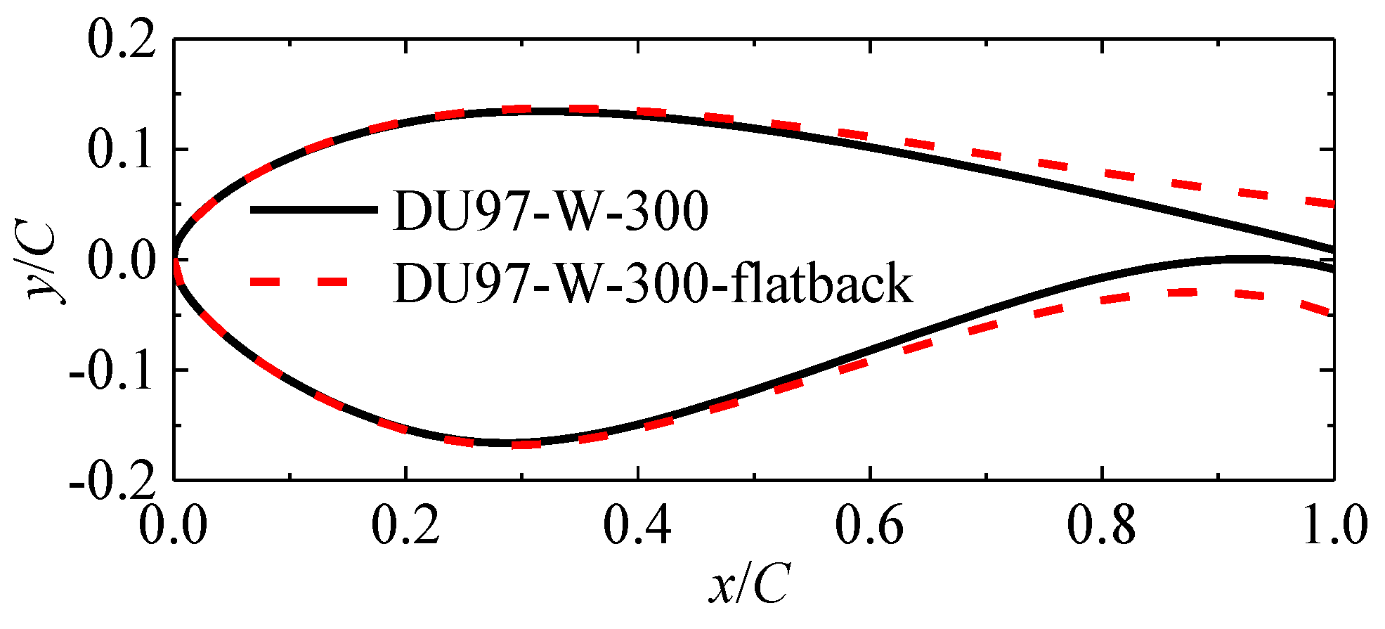
Figure 3 presents the geometry of the DU97-W-300-flatback and DU97-W-300. The trailing edge thickness for the DU97-W-300-flatback airfoil is 10%, and the thickness of the airfoil is 30%. The trailing edge thickness of the DU97-W-300 airfoil is 1.74%, and the thickness is 30%.

3. Results and Discussion

3.1. Validation of Aerodynamic and Aero-Acoustic Results

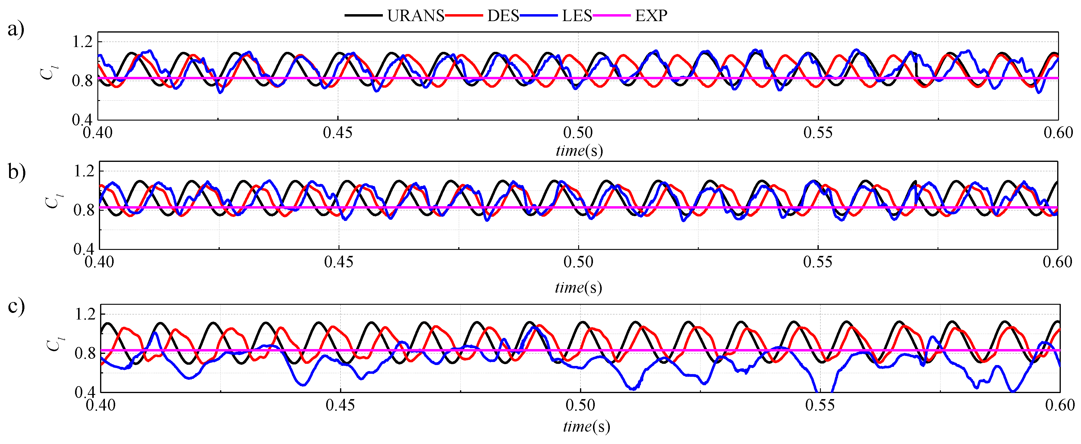
In order to verify the accuracy of the numerical results, a comparison was made with experiment data for the DU97-W-300-flatback airfoil from the Sandia National Laboratories wind tunnel measurements [47]. Figure 4 shows the comparison curves from numerical and experimental results. In the figure, the abscissa is time and the ordinate is the lift coefficient. The lift coefficient from numerical computations is transient and varies with time, while the experimental value is a time-averaged value. Figure 4a–c shows the calculation results for Mesh 1, Mesh 2 and Mesh 3, respectively. From Figure 4a, the results of URANS and DES present the regular periodic fluctuation. The LES calculation also shows a relatively regular fluctuation, but the periodicity is slightly worse than the other two methods. The variation of Figure 4b is similar to Figure 4a. Figure 4c is obtained from Mesh 3 with 280,000 mesh elements. URANS and DES results are close to each other, but the LES results deviate greatly from that of the former two methods. LES calculation results are lower than other two methods, and the periodicity is poor. For LES calculated results, Mesh 1 and Mesh 2 are closer together. However, the results of Mesh 3 differ greatly, the calculated value is lower, and the periodicity is poor.

The results of the mesh dependency study are shown in

Table 2. Results of the mesh independency study by turbulence calculation method.

Method	Mesh			Richardson Extrapolation (RE)
	Mesh 1	Mesh 2	Mesh 3	RE	p	R
URANS	0.9195	0.9225	0.908	--	--	−4.83
DES	0.9007	0.896	0.8952	0.8949	2.55	0.17
LES	0.9247	0.9121	0.7206	--	--	15.19

. RE represents the solution of the Richardson extrapolation [48], R is the ratio of errors, and p is the order of accuracy. The convergence conditions are: 0 < R < 1 (monotonic convergence); R < 0 (oscillation convergence); and 1 < R (divergence). For monotone convergence, the generalized Richardson extrapolation method can be used to estimate the errors. For oscillation convergence, the range of errors, i.e., uncertainty, can only be obtained from amplitude. For divergence, errors and uncertainty cannot be estimated. The results of URANS calculations belong to oscillatory convergence, and three sets of grids are insufficient to obtain extrapolation. There are two reasons for this result. One is that the calculation of the URANS model involves some turbulence model constants, which are calibrated by simple wall boundary layer flow and channel flow. However, for complex flows such as transition separation, these calibration parameters may need to be revised. Secondly, there are truncation errors and iteration errors in the numerical calculation process. When the mesh is refined, the truncation error of numerical calculation will decrease, but the iteration error will increase. In the sense of grid convergence study, the adopted grid does not enter the asymptotic convergence region of the numerical solution. LES results are divergent, and the extrapolation values of the three sets of grids cannot be obtained at present. The LES model separates large-scale eddies from small-scale eddies by filtering functions. Eddies larger than the grid size can be directly calculated by the Navier-Stokes equation, while small-scale eddies can be closed by the sub-lattice model. Small-scale eddies only play a dissipative role, and they are almost isotropic. When the number of grids is small, most of the vortices in the boundary layer are closed by the sub-lattice model, while those outside the boundary layer are simulated directly, so the two results are close. However, when the number of grids continues to be refined, because the grid scale in the boundary layer is very small, many eddies at the bottom of the boundary layer will be calculated by the direct numerical simulation method. The vortices generated by fluid shearing at the bottom of the boundary layer have the characteristic of spreading direction, and the two-dimensional calculation is used in this calculation, which will produce false strong shedding vortices at the bottom of the airfoil boundary layer. This is a numerical phenomenon rather than a physical one (Figure 5). Hence, results of LES are divergent in the study of grid convergence. The DES method uses the URANS method in the near-wall area and the LES model in the main flow area; the results of DES are monotonically convergent to the mesh. As illustrated in Figure 4, the numerical results obtained from Mesh 3 can predict the experimental lift coefficient well. Therefore, this higher resolution Mesh 3 was used for the current computations.

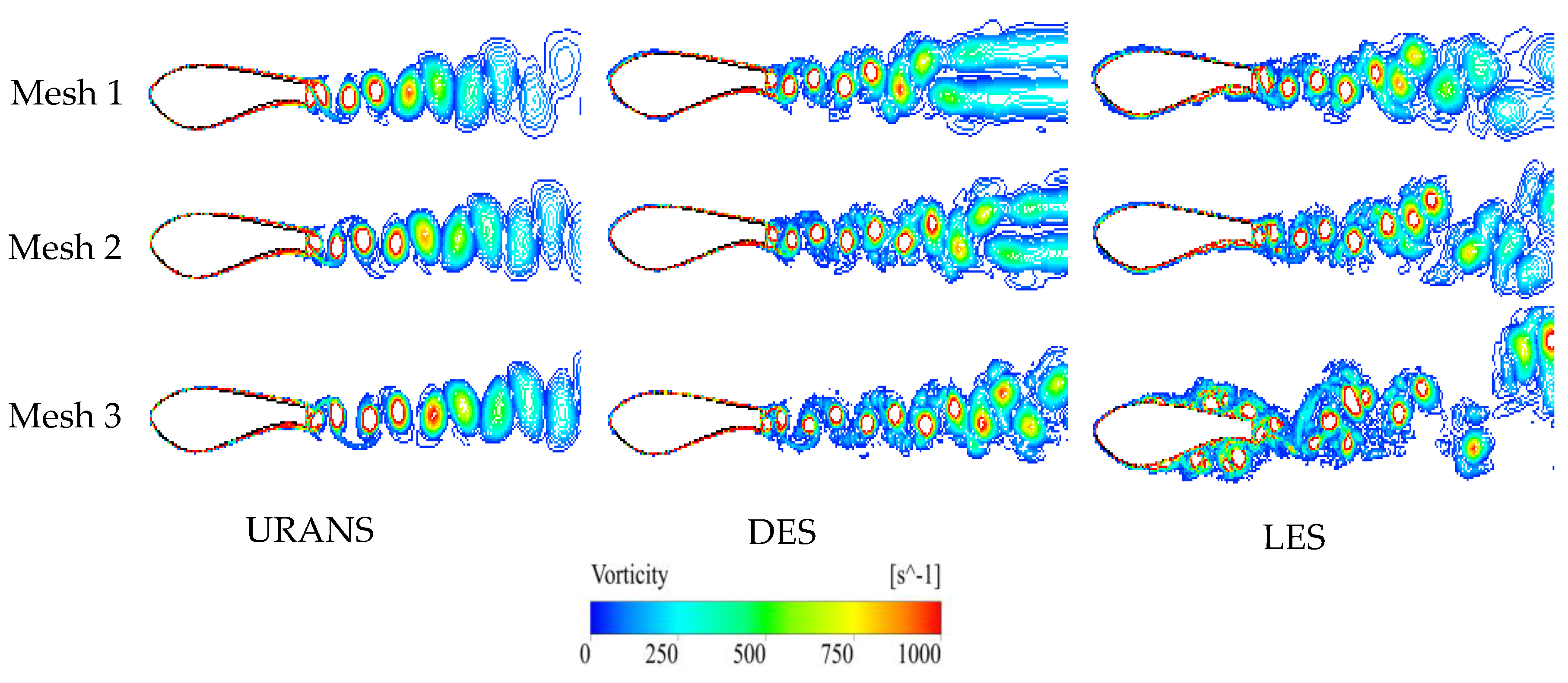
Figure 5 presents the vortex contours for different mesh numbers and turbulence calculation methods. It can be seen that both the vortex scales and the distance between the vortex nuclei for URANS are larger than that of the other two methods. The vortex scales calculated by LES are smaller, and the distance between the vortex nuclei is short. DES produced results that are between URANS and LES. From the results for the different mesh, it is found that the difference between Mesh 1 and Mesh 2 is small.

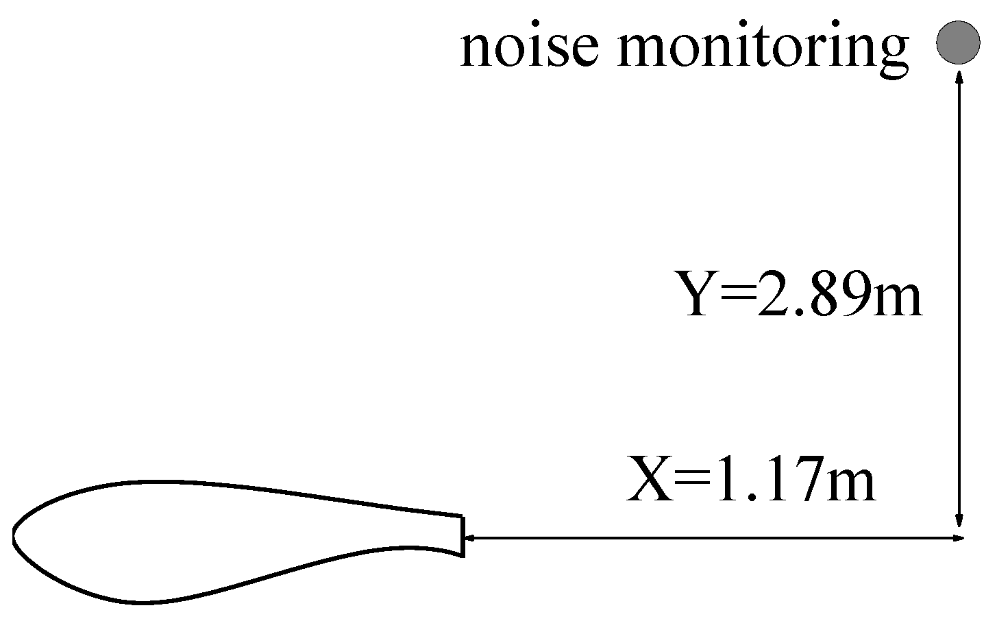
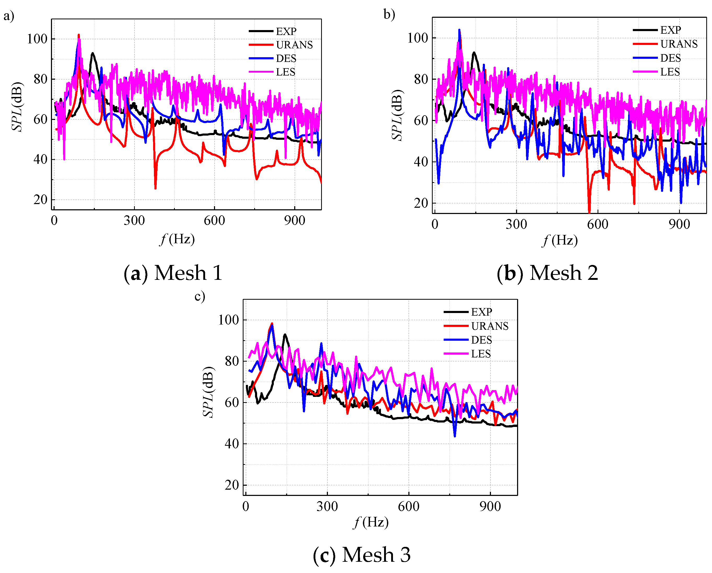
Figure 6 shows the position of the noise monitoring point for the airfoil, which is located 2.89 m above and 1.17 m downstream of the airfoil. Figure 7 shows the sound pressure level (SPL) distribution of the monitoring point. First, from Mesh 1, the results from all three turbulence models agree with a main SPL frequency of f ≈ 90 Hz, and a corresponding magnitude of SPL ≈ 100 dB. On the other hand, the experimental results have a main frequency of f ≈ 144 Hz, and a corresponding magnitude of SPL ≈ 93 dB. The numerical methods show greater magnitude fluctuations compared to the experiments. In Mesh 1 and 2, URANS produces the largest SPL fluctuations and underpredicts SPL. However, in Mesh 3, the fluctuations are greatly dampened, and SPL is overpredicted at high frequencies. Aside from the large increase in the number and magnitude of fluctuations in Mesh 2, DES consistently produces results that are close to the experimental results in all three meshes. Moreover, LES consistently overpredicts SPL at high frequencies for all three meshes. In Mesh 1 and 2, LES produces much more SPL fluctuation, but the fluctuation is dampened in Mesh 3. In Mesh 3, the three turbulence models produce results that are most agreeable with each other and with the experiments. The SPL fluctuations and their magnitudes are also generally the same for all three turbulence models. In addition, with more mesh elements, the models generally overpredict SPL at high frequencies.

3.2. Noise Analysis of Blunt Trailing Edge Airfoils

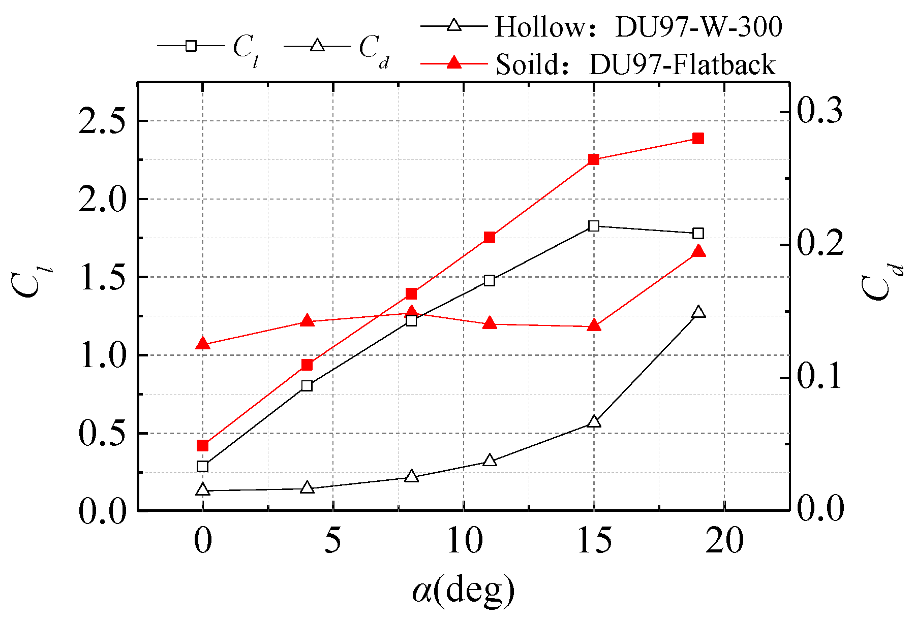
From the above analysis, it can be seen that the DES calculation is better than URANS and LES calculation results in terms of both the lift coefficient and noise SPL distribution of airfoil. Thus, the DES method and the Mesh 3 distribution were used for the current numerical computations. The calculation settings are the same as those in Section 2.1.3. The lift and drag coefficients are averaged over time to compare the effects of trailing edge thickness on lift and drag coefficients of airfoils. Figure 8 shows the lift and drag coefficient distribution of the airfoil. In this figure, the curves of the hollow markers represent the DU97-W-300 airfoil and the curves of the solid markers represent the DU97-Flatback airfoil. Firstly, the lift coefficient of the BTE airfoil is higher than that of the original airfoil, whether at small angle of attack or at large angle of attack. The stall angle of attack of the BTE airfoil is also larger than that of the original airfoil. With the increase of attack angle, the difference between lift coefficient of the BTE airfoil and that of the original airfoil becomes larger. Secondly, for the drag coefficient, the drag coefficient of the BTE airfoil is higher than that of the original airfoil, which is different from the lift coefficient. The smaller the angle of attack, the greater the difference between the drag coefficient of the BTE airfoil and that of the original airfoil. The drag coefficient of the BTE airfoil only shows a small change from 0° to 15° AOA. However, for the original DU97-W-300 airfoil, the drag coefficient increases gradually with the increase of AOA.

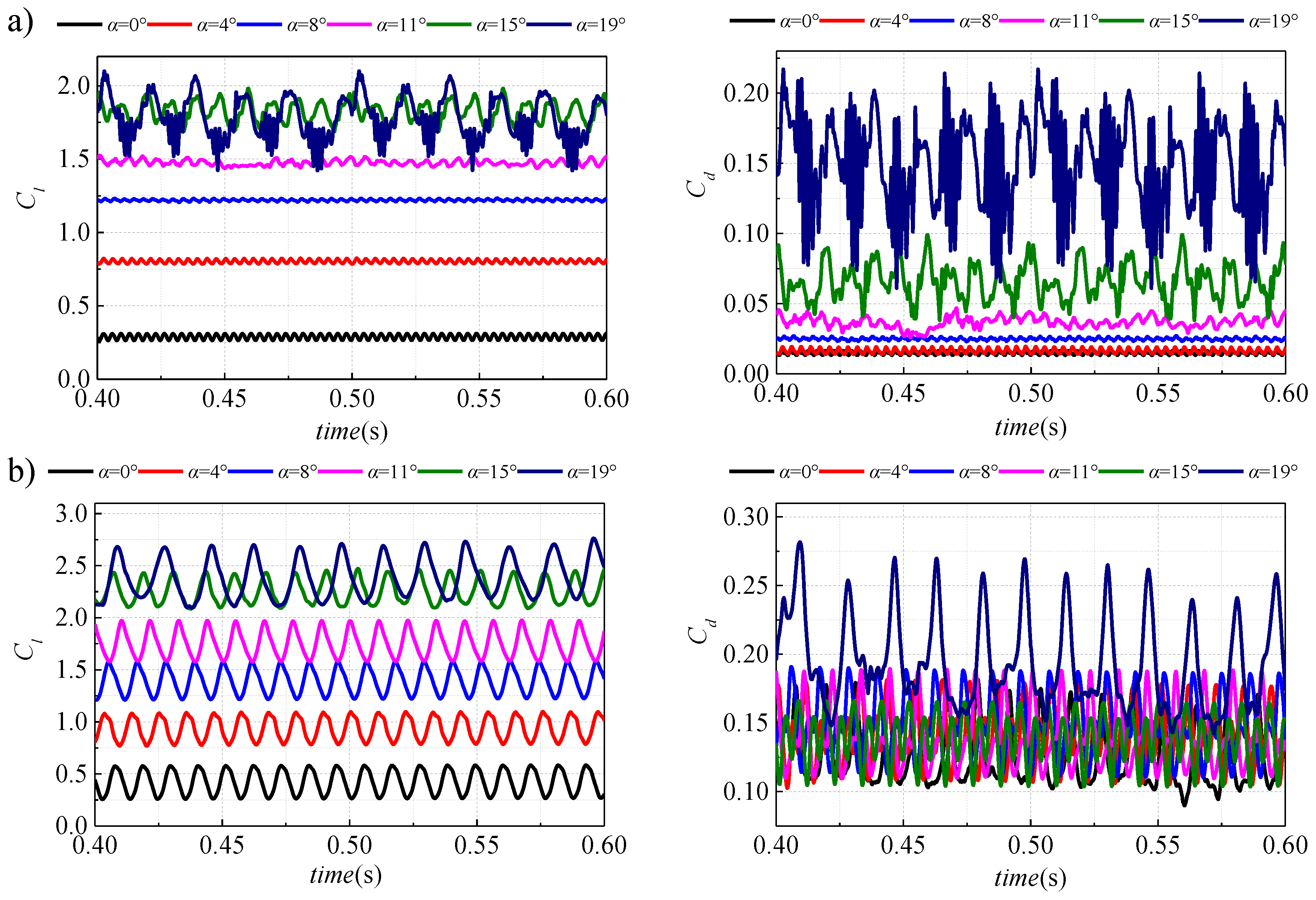
Figure 9 shows the lift and drag coefficient change curves for the airfoil over time. Figure 9a is the original airfoil, and Figure 9b is the BTE airfoil. From Figure 9a, the amplitude of the lift coefficient increases with AOA, and the fluctuation is the largest at 15° and 19° AOA. The amplitude of the drag coefficient increases with the increase of the AOA. At 19° AOA, the drag coefficient fluctuates drastically, and this indicates that the airfoil has stalled. Meanwhile, the effect of the turbulent separation vortex on the aerodynamic performance of the airfoil is obvious. For the BTE airfoil, the lift and drag coefficient fluctuates greatly at all AOA. From the comparison of Figure 9a,b it can be found that the fluctuation is very small for the original airfoil, while fluctuation of the BTE airfoil is very large. This is because the strength of the trailing edge vortex is weak for the original airfoil, thus, the force acting on the airfoil is very small. For the BTE airfoil, since the trailing edge thickness is larger, the strength of the trailing edge vortex is also larger. This vortex has strong periodic force on the airfoil, causing the periodic oscillation lift and drag coefficient.

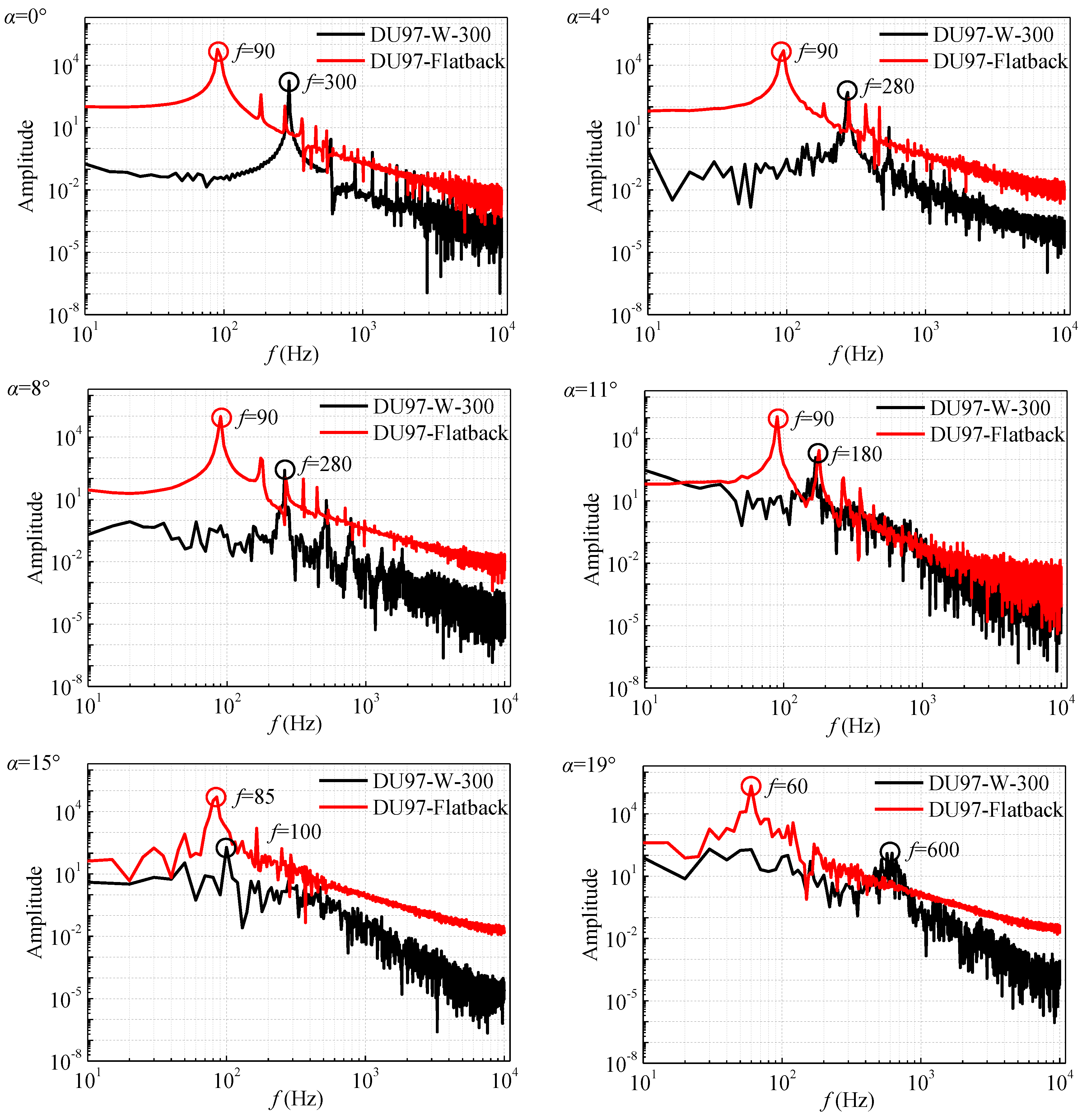
Figure 10 shows the power spectra distribution of the lift coefficient. The figure shows that the main frequency of the BTE airfoil is always lower than that of the original airfoil. From 0–15° AOA, the main frequency of the BTE airfoil is generally constant. At 19° AOA, the main frequency reduces to 60 Hz, and the main frequency variation pattern of the original airfoil is rather complicated. The main reasons for the result are that all the forces acting on the BTE airfoil are mainly induced by the trailing edge vortex, at 0–15° AOA. The trailing vortex has a dominant effect on the forces acting on the airfoil. At 19° AOA, there is large-scale flow separation on the suction face of the BTE airfoil. Here, both the trailing and separated vortices affect the forces acting on the airfoil. For the original airfoil, the smaller trailing edge thickness produces a weaker trailing edge vortex and has less effect on surface forces. These forces are, however, more heavily influenced by the surface vortices in the boundary layer, which changes drastically with the AOA.

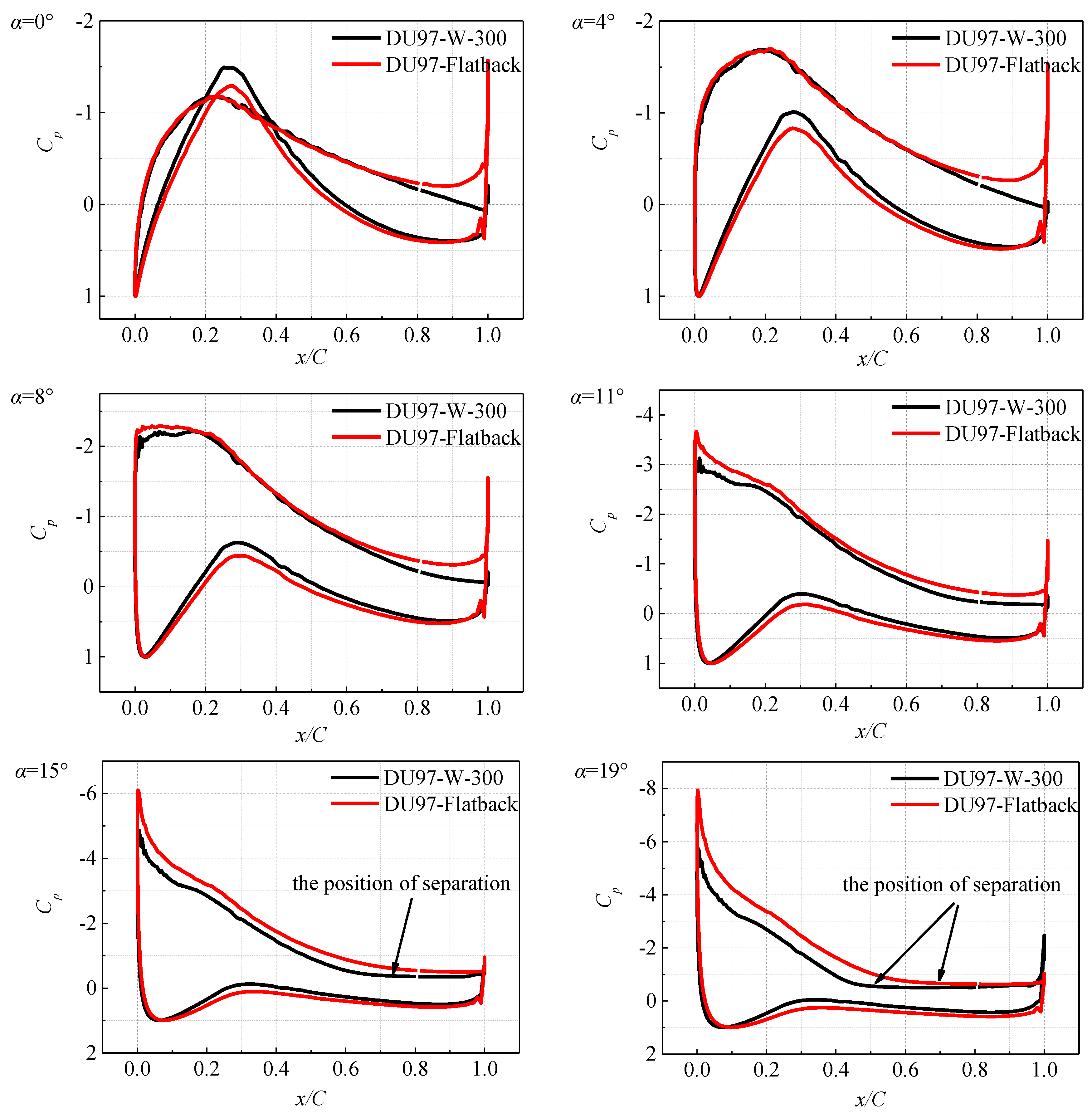
Figure 11 compares the distribution of the pressure coefficient (C_p). At 0–11° AOA, the distribution of C_p presents a slight difference between the original and BTE airfoils. At 15° AOA, the original airfoil produces a small pressure plateau on the suction face, which indicates that separation has occurred and the airfoil has entered its initial stages of stall. Conversely, the BTE airfoil has not stalled. At 19° AOA, both airfoils showed a pressure plateau near the trailing edge and are experiencing stall. However, the BTE airfoil has a relatively smaller plateau which begins at close to 0.7C, compared to that of the original airfoil which begins at about 0.5C. This implies that the flow on the suction face of the BTE airfoil separated later, closer to the trailing edge.

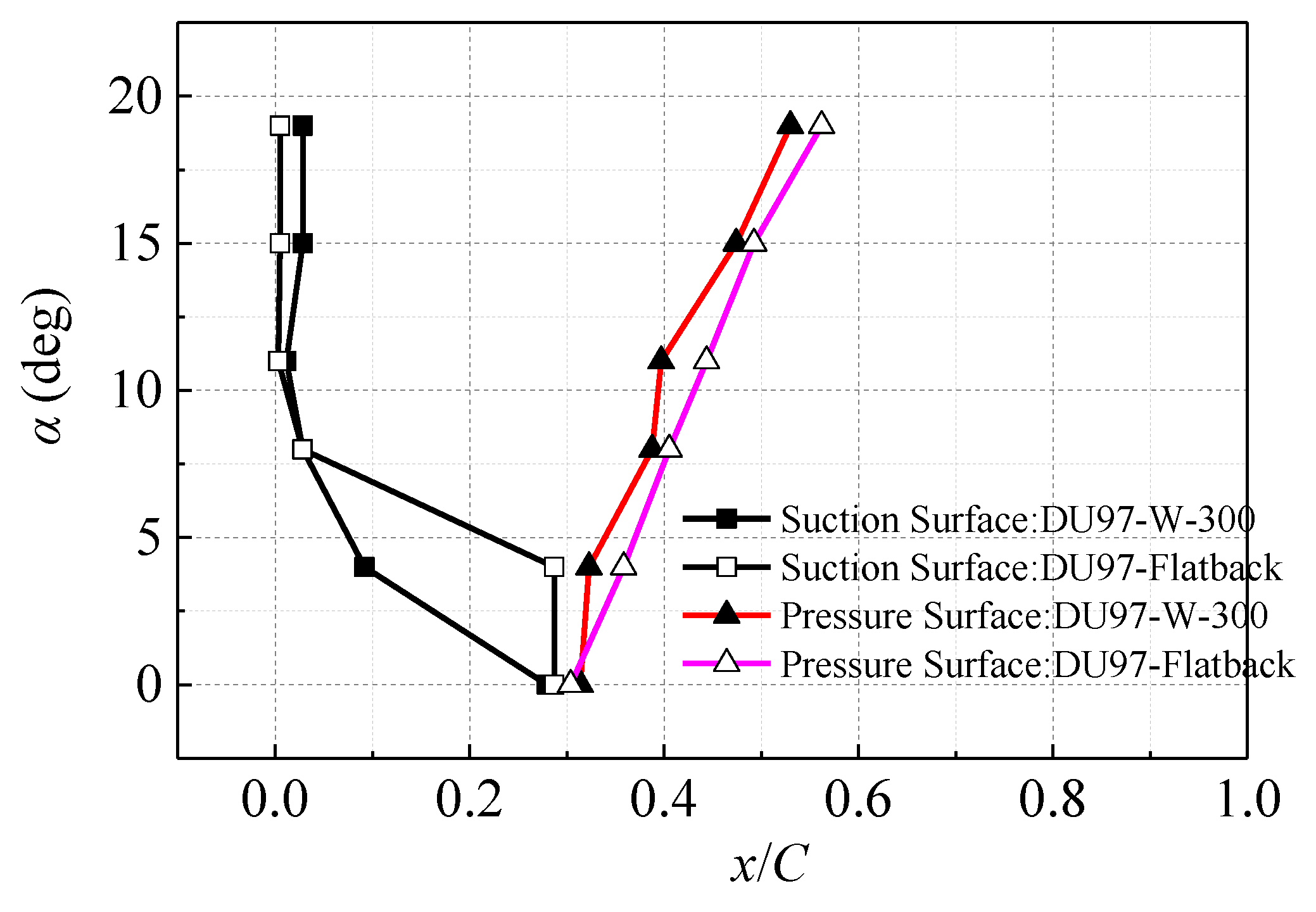
Figure 12 shows the distribution of the transition location on the airfoil suction and pressure surface. At 0° AOA, the position of transition is very close for the two airfoils. At 4° AOA, for the BTE airfoil, the position of transition on the suction surface is located at 0.28C, while for the original airfoil, the position of transition is at 0.1C. With the increase of AOA, the transition position for the BTE airfoil on the suction surface is closer to the leading edge than that of the original airfoil, and the result indicates that the transition is more likely to occur on the suction surface for a BTE, compared with the original airfoil. On the pressure surface, the transition position for the original airfoil is closer to the leading edge than that of the BTE airfoil.

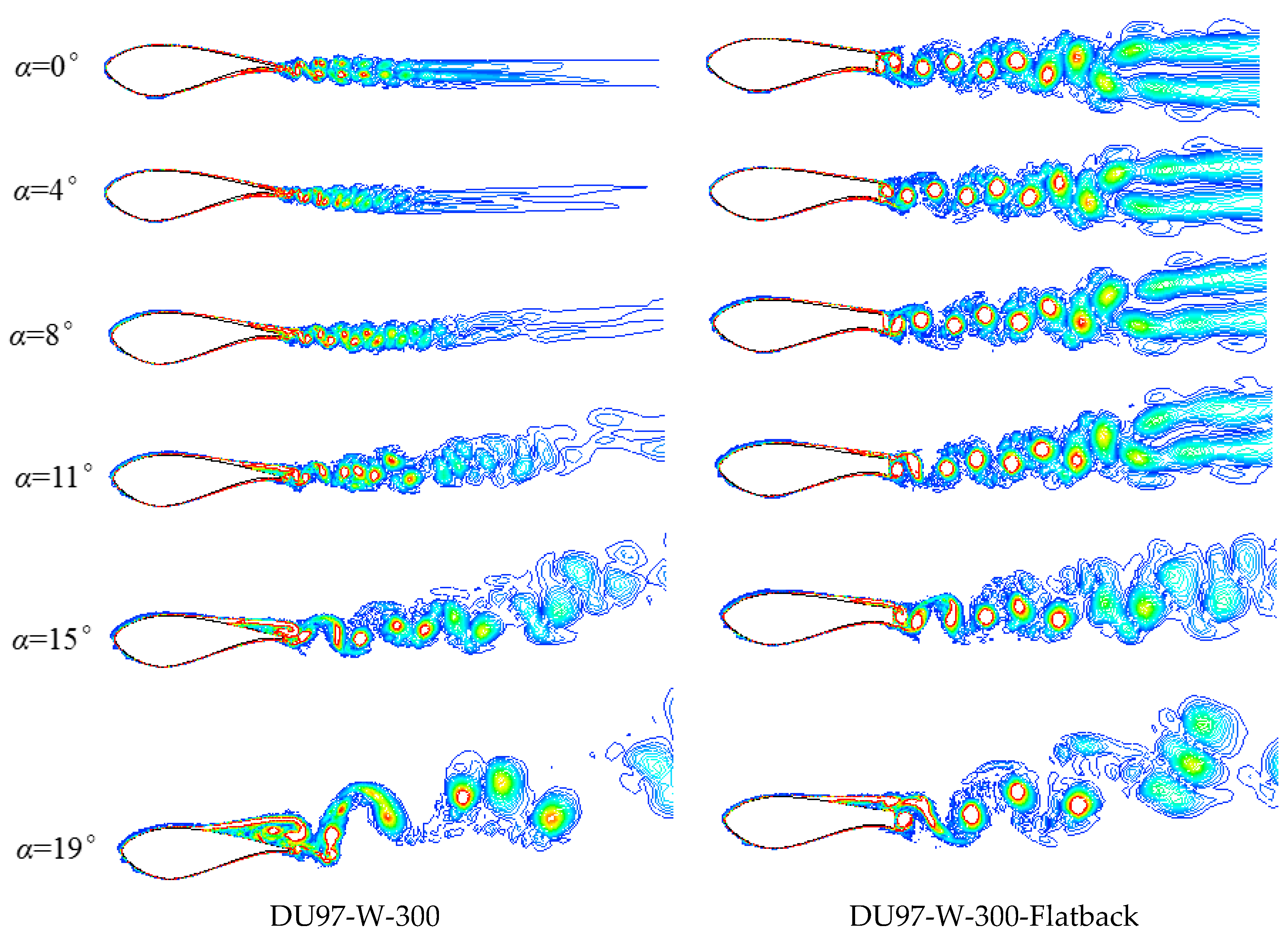
Figure 13 shows the vorticity contours of the two airfoils. At a small AOA (0°, 4°, 8°), the trailing edge shedding vortex scale of the original airfoil is small, and the frequency is high. For the BTE airfoil, the trailing edge shedding vortex scale is large and the frequency is low. When the angle of attack reaches 11°, flow separation appears at the trailing edge of the original airfoil. When the AOA reaches 19°, the wake of the original airfoil is mainly induced by the large-scale separation vortex on the suction surface, while the wake of the BTE airfoil is still largely shaped by the vortices shed from the trailing edge. The results show the distinct characteristics of the flow around the two airfoils being studied. This can help to explain the differences in aerodynamic noise generated by these airfoils.

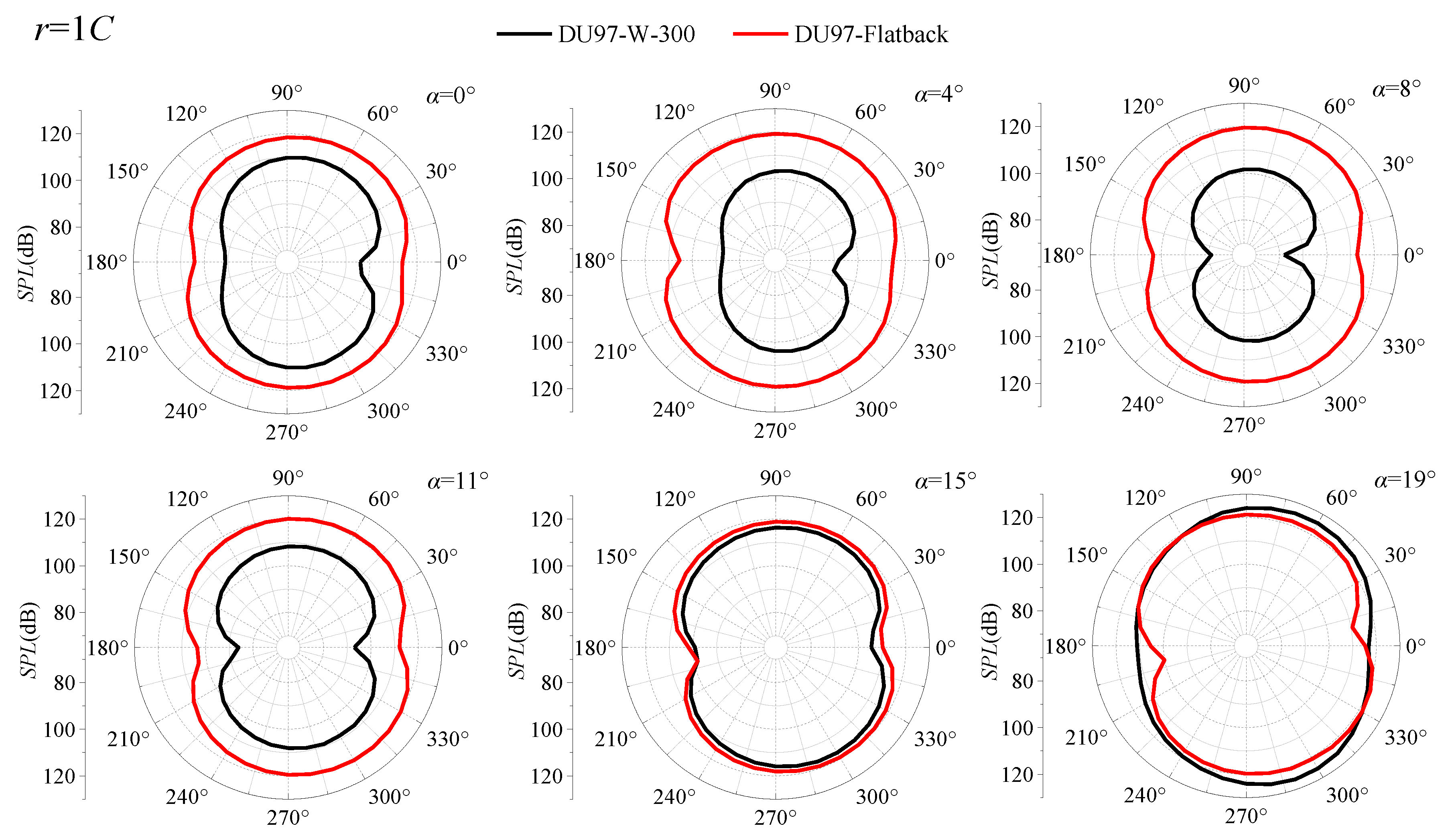
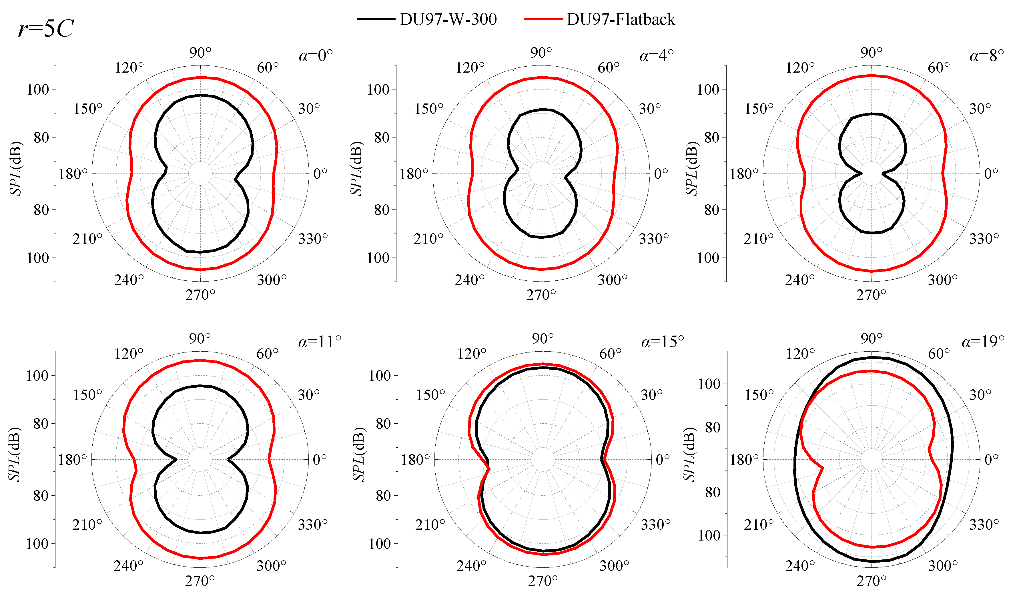
Figure 14 shows the distribution of noise monitoring points. Thirty-five monitoring points were arranged in one circle of airfoil, with a 10° interval between each monitoring point. Five circle monitoring points were set up in the radial direction, with each circle monitoring point at a distance 1C. Figure 15 presents the directional distribution curves of the SPL. From the SPL shape distribution in Figure 15, the BTE and original airfoils showed a dipole source. At 0° AOA, the original airfoil has a small sound pressure loss area near the trailing edge. As such, the noise generated by the trailing edge vortex is relatively small. For the BTE airfoil, the loss area of the SPL is most significant near the leading edge. As such, the noise generated by the leading-edge boundary layer also has a small effect. At 0–11° AOA, the SPL of the original airfoil is smaller than that of the BTE airfoil. As AOA increases, the SPL of the original airfoil increases and becomes closer to that of the BTE airfoil. At 19° AOA, the pressure level of the original airfoil becomes larger than that of the BTE airfoil.

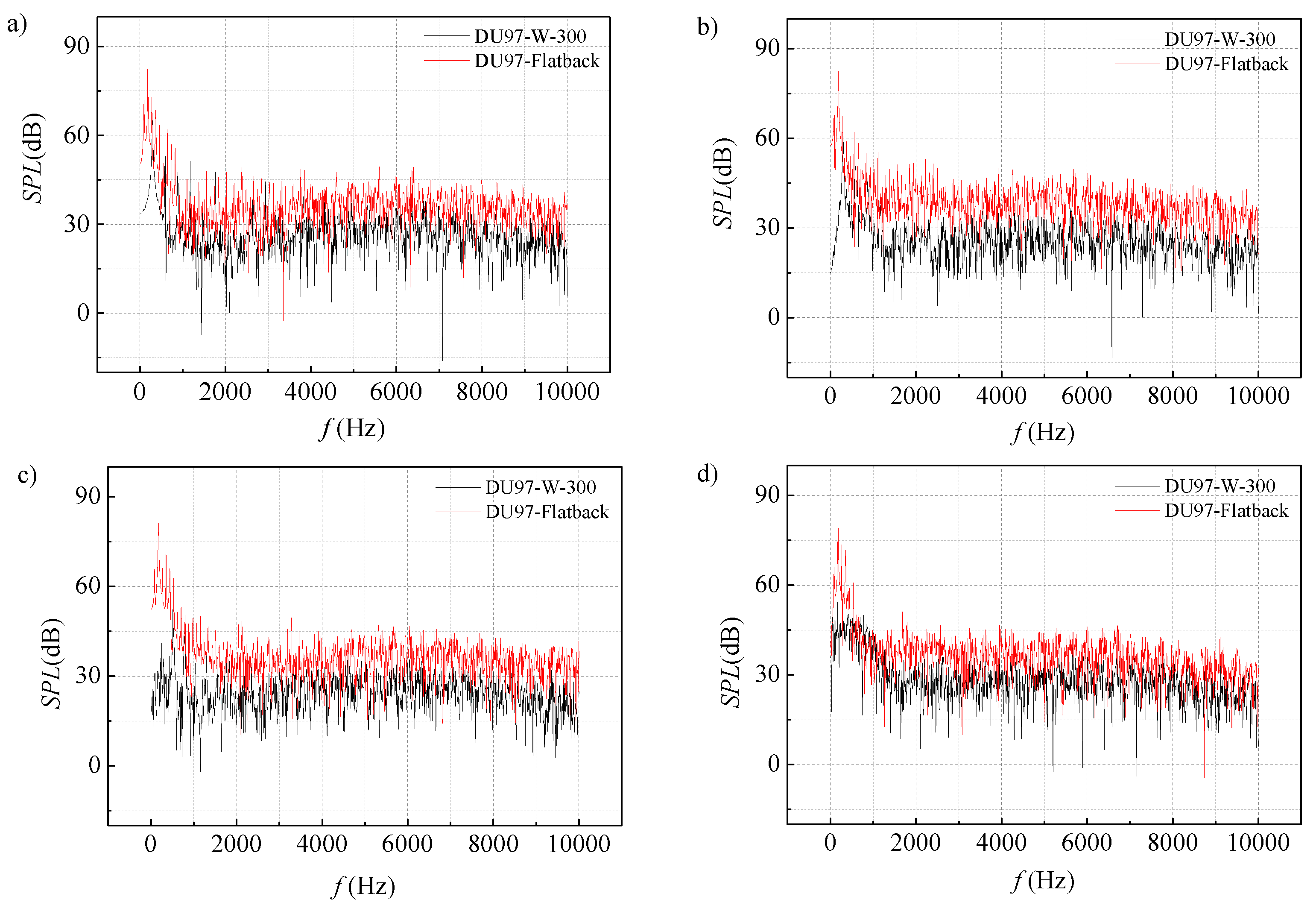
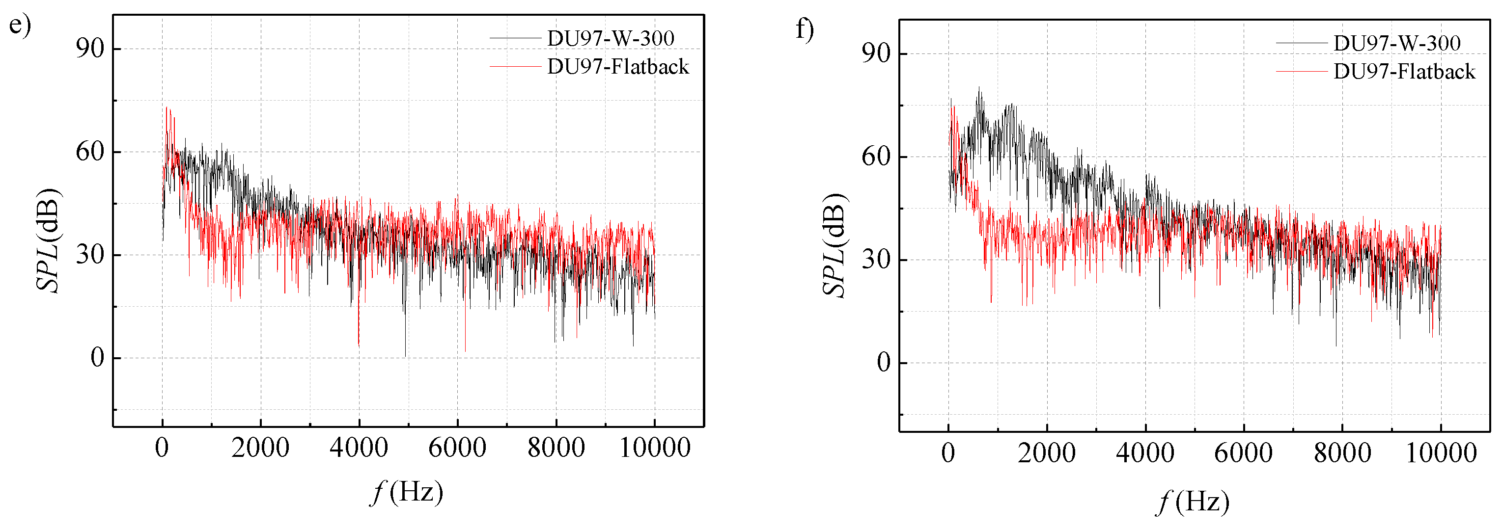
Figure 16 shows the spectrum of the SPL. At 0–11° AOA, the distribution of the SPL in the original airfoil shows a distinct peak in the low frequency region, thus, exhibits low frequency characteristics. At the higher AOAs of 15° and 19°, the SPL distribution shows more broadband characteristics as turbulent separation becomes the dominant source of noise. Similarly, at 0–19° AOA, the BTE airfoil also shows a distinct peak in the low frequency region and exhibits low frequency characteristics. The thicker trailing edge thickness in the BTE airfoil produces a stronger trailing edge vortex than the original airfoil. This allows the trailing vortex to become the dominant source of noise in a BTE airfoil through the range of AOA being studied.

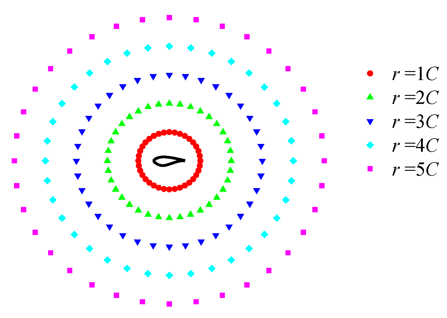
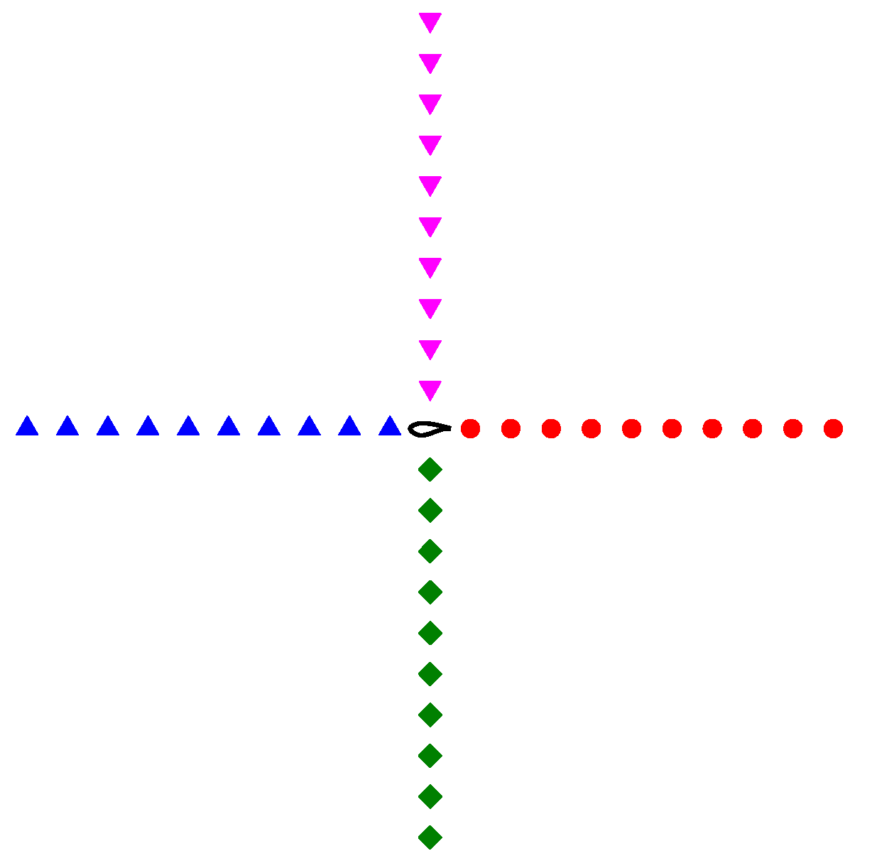
Figure 17 shows the distribution of noise monitoring points in four radial directions of the airfoils. The distance between each monitoring point is 1C. There are 10 monitoring points in each direction, totaling 40 monitoring points.

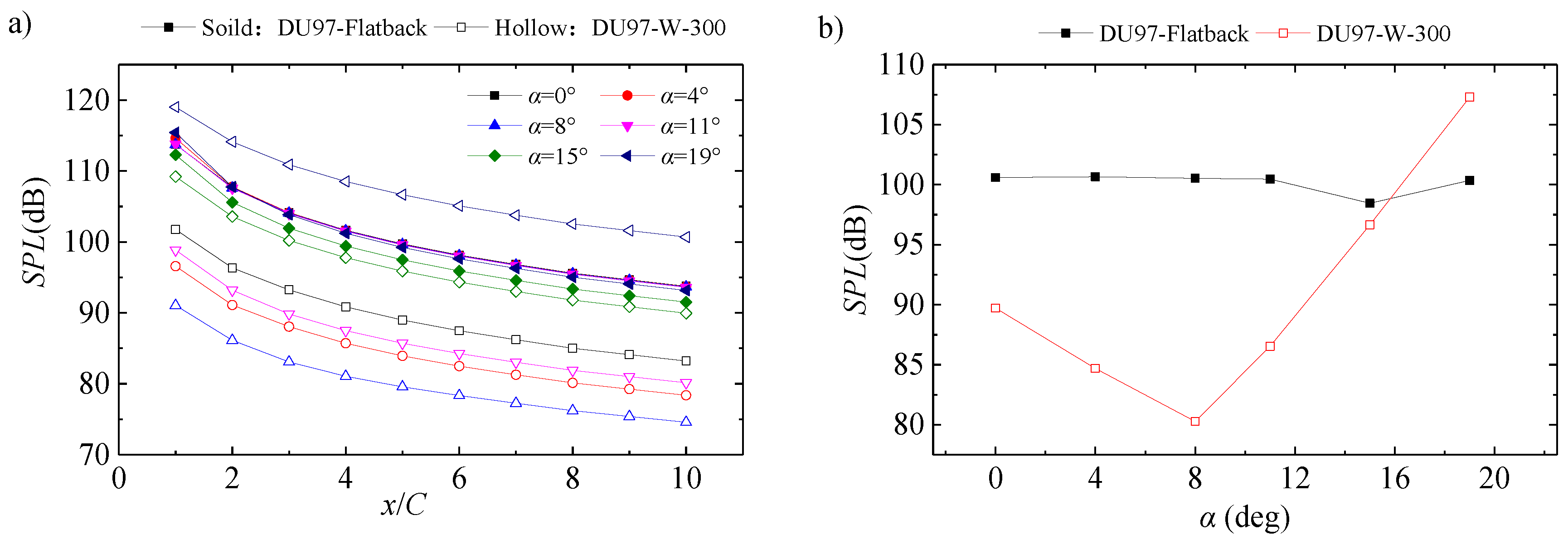
Figure 18 presents the total SPL distribution of the airfoils. Figure 14a indicates the average value of SPL in four directions; the total SPL decreases with the increase of distance. The total SPL of the BTE airfoil varies slightly at different AOAs, which is different from the results of the original airfoil. Figure 14b shows that the total SPL of the BTE airfoil remains relatively constant through the entire range of AOA from 0° to 19°. However, the original airfoil produces much larger variations in total SPL. The BTE airfoil has the largest and smallest SPL at 4° and 15° AOA, respectively. Conversely, for the original airfoil, the largest SPL occurs at 19° AOA and the smallest SPL occurs at 8° AOA.

The root-mean-squared (RMS) pressure fluctuation P_rms is considered a measure of the strength of sound sources [49], and is defined as the following:

$$P_{rms}=\sqrt{\left({\displaystyle \underset{0}{\overset{T}{\int }}{\left(p-\overline{p}\right)}^{2}dt}\right)}/T$$

(49)

where p is the instantaneous pressure, $\overline{p}$ is the time-averaged pressure and T denotes the integration time.

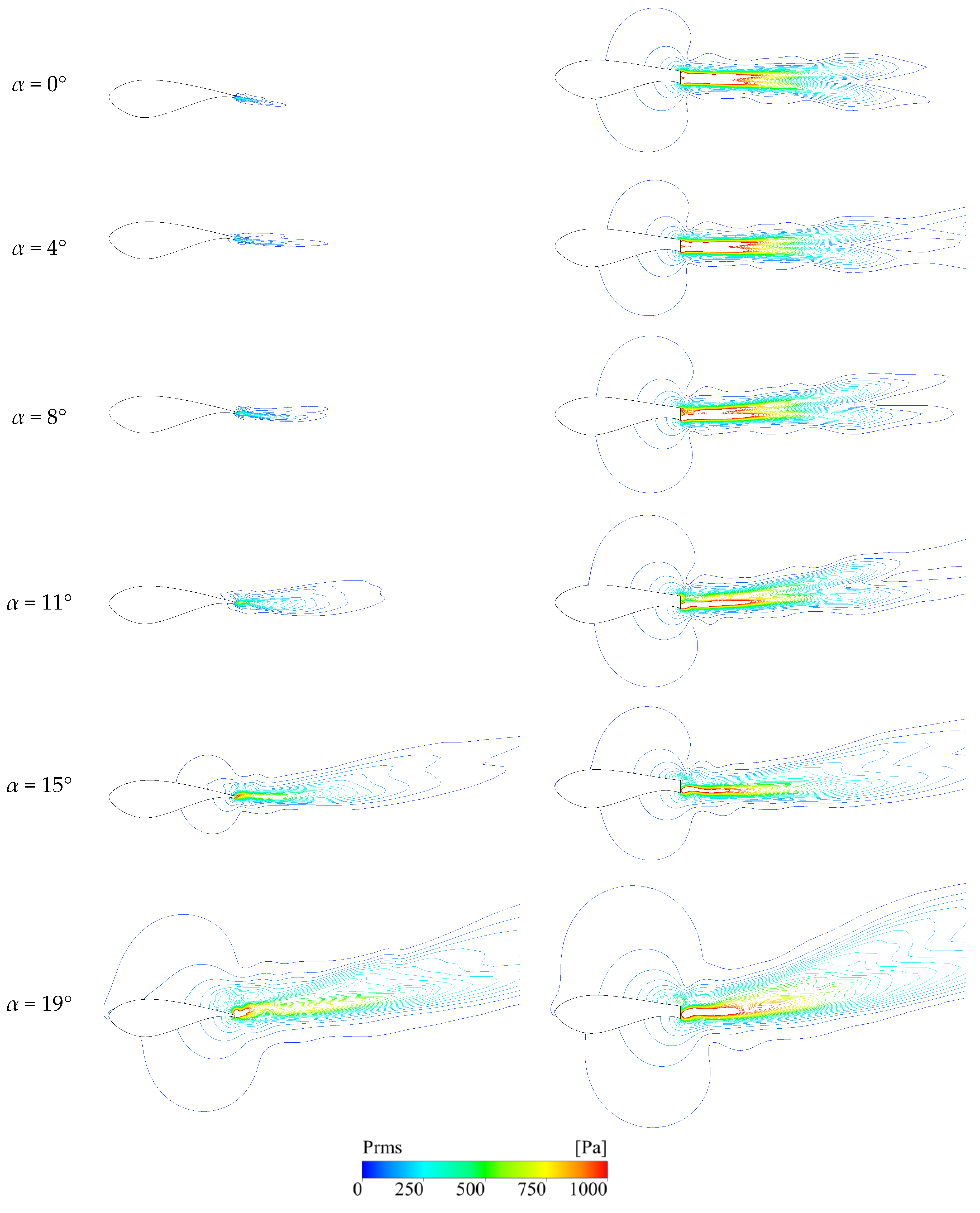
Figure 19 shows the contours of RMS pressure. In general, the noise source of the two airfoils is concentrated near the trailing edge. The peak RMS pressure of the BTE airfoil is much larger than that of the original airfoil.

4. Conclusions

In this paper, the aerodynamic and noise characteristics of the DU97-W-300-flatback (BTE) airfoil have been studied. This research mainly focuses on the effects of three turbulence methods (URANS, DES, and LES) on airfoil aerodynamic noise. Then, the DU97-W-300 and DU97-W-300-flatback airfoils are used to investigate the influence of trailing edge thickness on aerodynamic performance and noise. The main conclusions from this study are as follows.

The main SPL frequency computed from all three turbulence models are similar, and the main SPL frequency computed is 54 Hz lower than the experimental results. The peak SPL from the numerical methods generally agrees with the experimental results, albeit is slightly higher than that of the experiment. The results also show that URANS and DES produce similar SPL levels when plotted against frequency, but DES results are closer to the experimental values. Compared with the three turbulence methods, the results of DES are slightly better than from the URANS and LES methods, whether in terms of the aerodynamic characteristics of the airfoil or the noise characteristics of the monitoring points.

The influence of trailing edge thickness on aerodynamics and noise of airfoils is studied by the DES method. The lift and drag coefficients of the BTE airfoil are higher than that of the original airfoil. The bigger the AOA, the bigger the difference in the lift coefficient. The lift coefficient of the BTE airfoil increases by about 66% and the drag coefficient increases by nearly 550% at the AOA of 0°, and the lift coefficient increases by about 37% and the drag coefficient increases by nearly 26% at the AOA of 19°. Hence, the blunt trailing edge airfoil increases the lift coefficient of an airfoil and the drag coefficient increases at the same time. The fluctuation amplitude of the lift–drag coefficient of the blunt trailing edge airfoil is larger than that of the original airfoil. However, the main frequency of the lift coefficient for the BTE airfoil is higher than that of the original airfoil. The main frequency of the lift coefficient of the BTE airfoil is 210 Hz higher than that of the original airfoil at 0° AOA, which is an increase of nearly 230%; at the AOA of 15°, the main frequency is 15 Hz higher than that of the original airfoil, an increase of nearly 17%. For the original airfoil, the distribution of SPL exhibits low frequency characteristics at a small AOA, while at a large AOA, the distribution of SPL shows broadband characteristics. For the BTE airfoil, the distribution of the SPL exhibits low frequency characteristics through the entire AOA range being studied. For the BTE airfoil, the AOAs of maximum and minimum SPL are 4° and 15°, respectively. For the original airfoil, the AOAs of maximum and minimum SPL are 19° and 8°, respectively. The total SPL of the BTE airfoil increases by 26% at the AOA of 8°, while the total SPL of the BTE airfoil decreases by 6.5% at the AOA of 19°. For most AOAs, the SPL of the BTE airfoil is greater than that of the original airfoil.

References

- Tian, W.; Ozbay, A.; Hu, H. An experimental investigation on the aeromechanics and wake interferences of wind turbines sited over complex terrain. J. Wind Eng. Ind. Aerodyn. 2018, 172, 379–394. [Google Scholar] [CrossRef]
- Liu, H.; Hayat, I.; Jin, Y.; Chamorro, L. On the Evolution of the Integral Time Scale within Wind Farms. Energies 2018, 11, 93. [Google Scholar] [CrossRef]
- Uchida, T. Numerical Investigation of Terrain-Induced Turbulence in Complex Terrain by Large-Eddy Simulation (LES) Technique. Energies 2018, 11, 2638. [Google Scholar] [CrossRef]
- Takayuki Kageyama, T.Y.; Sonoko, K.; Shinichi, S.; Hideki, T. Exposure-response relationship of wind turbine noise with self-reported symptoms of sleep and health problems A nationwide socioacoustic survey in Japan. Noise Health 2016, 18, 53–61. [Google Scholar] [CrossRef]
- Katinas, V.; Marčiukaitis, M.; Tamašauskienė, M. Analysis of the wind turbine noise emissions and impact on the environment. Renew. Sustain. Energy Rev. 2016, 58, 825–831. [Google Scholar] [CrossRef]
- Wang, S.; Wang, S. Impacts of wind energy on environment: A review. Renew. Sustain. Energy Rev. 2015, 49, 437–443. [Google Scholar] [CrossRef]
- Kaldellis, J.K.; Garakis, K.; Kapsali, M. Noise impact assessment on the basis of onsite acoustic noise immission measurements for a representative wind farm. Renew. Energy 2012, 41, 306–314. [Google Scholar] [CrossRef]
- Liu, W.Y. A review on wind turbine noise mechanism and de-noising techniques. Renew. Energy 2017, 108, 311–320. [Google Scholar] [CrossRef]
- Anicic, O.; Petković, D.; Cvetkovic, S. Evaluation of wind turbine noise by soft computing methodologies: A comparative study. Renew. Sustain. Energy Rev. 2016, 56, 1122–1128. [Google Scholar] [CrossRef]
- Onakpoya, I.J.; O’Sullivan, J.; Thompson, M.J.; Heneghan, C.J. The effect of wind turbine noise on sleep and quality of life: A systematic review and meta-analysis of observational studies. Environ. Int. 2015, 82, 1–9. [Google Scholar] [CrossRef]
- Taylor, J.; Eastwick, C.; Lawrence, C.; Wilson, R. Noise levels and noise perception from small and micro wind turbines. Renew. Energy 2013, 55, 120–127. [Google Scholar] [CrossRef] [Green Version]
- Wang, Z.; Tian, W.; Hu, H. A Comparative study on the aeromechanic performances of upwind and downwind horizontal-axis wind turbines. Energy Convers. Manag. 2018, 163, 100–110. [Google Scholar] [CrossRef]
- Lee, S.; Lee, S. Numerical and experimental study of aerodynamic noise by a small wind turbine. Renew. Energy 2014, 65, 108–112. [Google Scholar] [CrossRef]
- Xu, H.Y.; Dong, Q.L.; Qiao, C.L.; Ye, Z.Y. Flow Control over the Blunt Trailing Edge of Wind Turbine Airfoils Using Circulation Control. Energies 2018, 11, 619. [Google Scholar] [CrossRef]
- Lee, S.G.; Park, S.J.; Lee, K.S.; Chung, C. Performance prediction of NREL (National Renewable Energy Laboratory) Phase VI blade adopting blunt trailing edge airfoil. Energy 2012, 47, 47–61. [Google Scholar] [CrossRef]
- Wang, G.; Zhang, L.; Shen, W.Z. LES simulation and experimental validation of the unsteady aerodynamics of blunt wind turbine airfoils. Energy 2018, 158, 911–923. [Google Scholar] [CrossRef]
- Zhu, W.J.; Shen, W.Z.; Barlas, E.; Bertagnolio, F.; Sørensen, J.N. Wind turbine noise generation and propagation modeling at DTU Wind Energy: A review. Renew. Sustain. Energy Rev. 2018, 88, 133–150. [Google Scholar] [CrossRef]
- Paterson, R.W.; Vogt, P.G.; Fink, M.R.; Munch, C.L. Vortex noise of isolated airfoils. J. Aircr. 1973, 10, 296–302. [Google Scholar] [CrossRef]
- Brooks, T.F.; Hodgson, T.H. Trailing edge noise prediction from measured surface pressures. J. Sound Vib. 1981, 78, 69–117. [Google Scholar] [CrossRef]
- Lighthill, M. On sound generated aerodynamically: I. General theory. Proc. R. Soc. Lond. 1954, 222, 1–32. [Google Scholar] [CrossRef]
- Curle, N. The influence of solid boundaries upon aerodynamic sound. Proc. R. Soc. Lond. 1955, 231, 505–514. [Google Scholar] [CrossRef]
- Ffowcs-Williams, J.E.; Hawkings, D.L. Sound generation by turbulence and surfaces in arbitrary motion. Philos. Trans. R. Soc. Lond. 1969, 264, 321–342. [Google Scholar] [CrossRef]
- Francescantonio, P.D. A new boundary integral formulation for the prediction of sound radiation. J. Sound Vib. 1997, 202, 491–509. [Google Scholar] [CrossRef]
- Singer, B.A.; Brentner, K.S.; Lockard, D.P. Simulation of acoustics scatting from a trailing edge. J. Sound Vib. 2000, 230, 541–560. [Google Scholar] [CrossRef]
- Ewert, R.; Schröder, W. On the simulation of trailing edge noise with a hybrid LES/APE method. J. Sound Vib. 2004, 270, 509–524. [Google Scholar] [CrossRef]
- Shen, W.Z.; Michelsen, J.A.; Sørensen, J.N. A collocated grid finite volume method for aeroacoustic computations of low-speed flows. J. Comput. Phys. 2004, 196, 348–366. [Google Scholar] [CrossRef]
- Sandberg, R.D.; Jones, L.E. Direct numerical simulations of airfoil self-noise. Proc. Eng. 2010, 6, 274–282. [Google Scholar] [CrossRef] [Green Version]
- Ikeda, T.; Atobe, T.; Takagi, S. Direct simulations of trailing-edge noise generation from two-dimensional airfoils at low Reynolds numbers. J. Sound Vib. 2012, 331, 556–574. [Google Scholar] [CrossRef]
- Albarracin, C.A.; Marshallsay, P.; Brooks, L.A.; Cederholm, A.; Chen, L.; Doolan, C.J. Comparison of aeroacoustics predictions of turbulent trailing edge noise using three different flow solution. In Proceedings of the 18th Australasian Fluid Mechanics Conference, Launceston, Australia, 3–7 December 2012. [Google Scholar]
- Lummer, M.; Delfs, J.W.; Lauke, T. Simulation of sound generation by vortices passing the trailing edge of airfoils. In Proceedings of the 8th AIAA/CEAS Aeroacoustics Conference & Exhibit, AIAA 2002, Breckenridge, CO, USA, 17–19 June 2002; pp. 2002–2578. [Google Scholar]
- Jones, L.E.; Sandberg, R.D. Numerical analysis of tonal airfoil self-noise and acoustic feedback-loops. J. Sound Vib. 2011, 330, 6137–6152. [Google Scholar] [CrossRef]
- Shin, H.; Kim, H.; Kim, T.; Kim, S.H.; Lee, S.; Baik, Y.J.; Lee, G. Numerical Analysis of Flatback Trailing Edge Airfoil to Reduce Noise in Power Generation Cycle. Energies 2017, 10, 872. [Google Scholar] [CrossRef]
- Fleig, O.; Arakawa, C. Numerical simulation of wind turbine tip noise. AIAA Aerosp. Sci. Meet. Exhib. 2013. [Google Scholar] [CrossRef]
- Fleig, O.; Iida, M.; Arakawa, C. Wind Turbine Blade Tip Flow and Noise Prediction by Large-eddy Simulation. J. Sol. Energy Eng. 2004, 126, 1017. [Google Scholar] [CrossRef]
- Marsden, O.; Bogey, C.; Bailly, C. Noise radiated by a high-Reynolds-number 3-D airfoil. In Proceedings of the Applied Aerodynamics Conference AIAA Paper, Toronto, ON, Canada, 6–9 June 2005; pp. 2005–2817. [Google Scholar]
- Jiang, M.; Li, X.D.; Bai, B.H.; Lin, D.K. Numerical simulation on the NACA0018 airfoil self-noise generation. Theor. Appl. Mech. Lett. 2012, 2, 052004. [Google Scholar] [CrossRef] [Green Version]
- Jiang, M.; Li, X.D.; Lin, D.K. Numerical Simulation on the Airfoil Self-Noise at Low Mach Number Flows. In Proceedings of the AIAA Aerospace Sciences Meeting Including the New Horizons Forum & Aerospace Exposition, Grapevine, TX, USA, 7–10 January 2013. [Google Scholar] [CrossRef]
- Takagi, Y.; Fujisawa, N.; Nakano, T.; Nashimoto, A. Cylinder wake influence on the tonal noise and aerodynamic characteristics of a NACA0018 airfoil. J. Sound Vib. 2006, 297, 563–577. [Google Scholar] [CrossRef]
- Nakano, T.; Fujisawa, N.; Oguma, Y.; Takagi, Y.; Lee, S. Experimental study on flow and noise characteristics of NACA0018 airfoil. J. Wind Eng. Ind. Aerodyn. 2007, 95, 511–531. [Google Scholar] [CrossRef]
- Jacob, M.C.; Jérôme, B.; Casalino, D.; Michard, M. A rod-airfoil experiment as a benchmark for broadband noise modeling. Theor. Comput. Fluid Dyn. 2005, 19, 171–196. [Google Scholar] [CrossRef]
- Björn, G.; Thiele, F.; Jacob, M.C.; Casalino, D. Prediction of sound generated by a rod–airfoil configuration using EASM DES and the generalised Lighthill/FW-H analogy. Comput. Fluids 2008, 37, 402–413. [Google Scholar] [CrossRef]
- Giret, J.C.; Sengissen, A.; Moreau, S.; Jouhaud, J.C. Prediction of sound generated by a rod-airfoil configuration using a compressible unstructured LES solver and a FW-H analogy. In Proceedings of the 8th AIAA/CEAS Aeroacoustics Conference & Exhibit, AIAA 2002, Breckenridge, CO, USA, 17–19 June 2002; pp. 2012–2058. [Google Scholar]
- Smagorinsky, J. General Circulation Experiments with the Primitive Equations, Part 1, Basic Experiments. Mon. Weather Rev. 1963, 91, 99–164. [Google Scholar] [CrossRef]
- Menter, F.R. Two-equation eddy-viscosity turbulence models for engineering applications. AIAA J. 1994, 32, 1598–1605. [Google Scholar] [CrossRef] [Green Version]
- Langtry, R.B.; Menter, F.R. Transition Modeling for General CFD Applications in Aeronautics. AIAA Aerosp. Sci. Meet. Exhib. 2005. [Google Scholar] [CrossRef]
- Spalart, P.R.; Jou, W.H.; Strelets, M. Comments on the Feasibility of LES for Wings, and on a Hybrid RANS/LES Approach. In Proceedings of the 1st Air Force Office of Scientific Research International Conference on DNS/LES, Ruston, LA, USA, 4–8 August 1997; pp. 137–147. [Google Scholar]
- Barone, M.F.; Berg, D.E.; Devenport, W.J.; Burdisso, R. Aerodynamic and Aeroacoustic Tests of a Flatback Version of the DU97-W-300 Airfoil; SAND2009-4185, Sandia Report; Sandia National Laboratories: Albuquerque, NM, USA, 2009. [Google Scholar]
- John, C.V.; Edward, N.T.; Mori, M.; Ben, R. Summary of the fourth AIAA computational fluid dynamics drag prediction workshop. J. Aircr. 2014, 51, 1070–1089. [Google Scholar] [CrossRef]
- Qiang, Z. Aerodynamic Acoustic Basis; National Defense Industry Press: Beijing, China, 2012. [Google Scholar]
Figure 1.
Computational mesh.
Figure 2.
Computational domain size and boundary condition.
Figure 3.
Airfoil geometry.
Figure 4.
Convergence history of lift coefficient: (a) Mesh 1, (b) Mesh 2, and (c) Mesh 3. URANS represents the results of unsteady Reynolds average Navier-Stokes method; DES represents the results of detached eddy simulation method; LES represents the results of large eddy simulation method; EXP represents the results of experimental.
Figure 5.
Vortices contours.
Figure 6.
Position of noise monitoring point.
Figure 7.
The sound pressure level (SPL) distribution at the monitoring point.
Figure 8.
Distribution of airfoil lift and drag coefficient.
Figure 9.
Change in rule of lift and drag coefficient with time. (a) DU97-W-300, (b) DU97-Flatback.
Figure 10.
Power spectra of lift and drag coefficient.
Figure 11.
Distribution of pressure coefficient on airfoil surfaces.
Figure 12.
Location of transition on the suction and pressure surfaces of the airfoils.
Figure 13.
Vorticity contours.
Figure 14.
The noise monitoring points of the airfoil.
Figure 15.
The directional distribution curves of SPL.
Figure 16.
Distribution of SPL: (a) α = 0°, (b) α = 4°, (c) α = 8°, (d) α = 11°, (e) α = 15°, (f) α = 19°.
Figure 17.
The noise monitoring points in four radial directions of the airfoils.
Figure 18.
Total SPL distribution of the airfoils: (a) The average value of SPL in four directions. (b) The total SPL.
Figure 19.
Contours of Prms.