Interpretation of Four Unique Phenomena and the Mechanism in Unsteady Flow Separation Controls


College of Energy and Power Engineering, Nanjing University of Aeronautics and Astronautics, Nanjing 210016, China
*
Author to whom correspondence should be addressed.
Energies 2019, 12(4), 587; https://doi.org/10.3390/en12040587
Submission received: 14 January 2019
/
Revised: 1 February 2019
/
Accepted: 7 February 2019
/
Published: 13 February 2019
Abstract
:Unsteady flow separation controls are effective in suppressing flow separations. However, the unique phenomena in unsteady separation control, including frequency-dependent, threshold, location-dependent, and lock-on effects, are not fully understood. Furthermore, the mechanism of the effectiveness that lies in unsteady flow controls remains unclear. Thus, this study aims to interpret further the unique phenomena and mechanism in unsteady flow separation controls. First, numerical simulation and some experimental results of a separated curved diffuser using pulsed jet flow control are discussed to show the four unique phenomena. Second, the bases of unsteady flow control, flow instability, and free shear flow theories are introduced to elucidate the unique phenomena and mechanism in unsteady flow separation controls. Subsequently, with the support of these theories, the unique phenomena of unsteady flow control are interpreted, and the mechanisms hidden in the phenomena are revealed.
1. Introduction
Flow separations often occur on airplane wings or compressor blades and result in lift losses or total pressure losses. In some serious cases, they may even cause airplane stall or engine surge. The use of design optimization technique of wings or blades effectively delays the occurrence of separation. However, for a near-stall wing or blade, the margin for design optimization to delay separations is small, whereas its difficulty is high. Thus, flow control methods are useful in suppressing or completely eliminating separation for fluid machinery with high-risk of flow separations. Unsteady flow controls are demonstrated to be more efficient than steady flow controls because less energy is needed to achieve the same control performance [1,2]. Typical unsteady flow control methods include acoustic excitation [3], synthetic jet [4], pulsed jet [5], wall oscillation [6], traveling wave wall [7] and plasma actuator [8] (see Table 1).
As nonlinear systems, unsteady flow separations with external excitations have many different characteristics from linear systems, as well as the existence of unique phenomena. On the basis of existing numerical and experimental results, the typical phenomena include frequency-dependent, threshold, position-dependent, and lock-on effects. Frequency-dependent effect indicates that the best control performance occurs when the external excitation frequency is near a certain value. Hence, an optimal non-dimensional external excitation frequency exists; this frequency is defined as , where is the external excitation frequency, is the distance from the excitation to the trailing edge of the wing or blade, and is the inflow velocity [1]. Seifert [9], Hsiao [10], and our study [11] also achieved similar results. Notably, frequency-dependent effect also exists in linear systems; for example, resonance in linear vibration depends on the excitation frequency but may share different mechanisms with unsteady flow control. Threshold effect means that only when the intensity of external excitation reaches a certain value or more can a significant control effect be achieved. This effect is a typical nonlinear one. In linear vibration, the response amplitude is simply proportional to the excitation amplitude, and no such threshold exists. The intensity of external excitation is often evaluated by the momentum coefficient . With regard to different cases (e.g., different geometries and Reynolds numbers), the threshold value of will vary from to [1]. Moreover, excessive may result in negative effects; therefore, the optimal value of is determined in some studies [9]. Location-dependent effect refers to the fact that the optimal location of external excitation is generally at or near the separation point. For example, excitation is usually applied at the shoulder of a defected flap or at the leading-edge of a sharp airfoil [1]. Another unique phenomenon in unsteady separation controls is the lock-on effect. Effective unsteady control with calibrated parameters is often accompanied by a lock-on effect, including phase- and frequency-lock [12]; otherwise, lock-on may not happen. However, in a linear vibration system, the vibration will consistently be locked to the excitation, regardless of the excitation frequency. This phenomenon indicates that effective control is related to the specific details of the coherent structures (no such structures lies in solids for vibration analysis). Thus, the understanding of these four unique phenomena is a key step in revealing the nonlinearity of unsteady flow separation controls.
Aside from the understanding of the phenomena, the mechanism of unsteady flow controls remains unclear [13]. However, widely accepted consensuses are observed on unsteady flow control. The first consensus is that periodic excitation is relevant with flow instability. Transition is related to Tollmein–Schlichting (T–S) waves generated by instability in laminar flows. In addition, flow instability, such as Kelvin–Helmholtz (K–H) instability, exists in turbulent flows. The external excitation with proper parameters can use flow instability and interact with coherent structures caused by instability [2]. On this basis, some unsteady flow control studies (e.g., acoustic excitation and pulsed jet flow control) use Orr–Sommerfeld (O–S) equation or its variants in linear stability theory to the quantitative analysis of flow instabilities [3,14]. Notably, although some weakly nonlinear stability theories (e.g., Stuart–Landau (S–L) theory [15]) can describe particular and simple phenomena, nonlinear stability theory remains immature. Another consensus is that excited free shear flow is the basis of unsteady flow control [1]. For typical wings and blades, although flow instabilities lie in the shear layer, separation bubbles, wakes and their coupling interactions [16], the free shear flow and its corresponding K–H instability are considered to be the most important and representative. From the theoretical and experimental studies of unexcited [17] and excited free shear flows [18], the relationship between the external excitation and coherent structures in the free shear layer is simple and well revealed in comparison with other complex flow structures (e.g., flow separations). Thus, flow instability and excited free shear flow are now the foundations of unsteady flow control, despite the vagueness of unsteady flow separation control mechanisms.
In this study, we initially present the four unique phenomena of pulsed jet flow control in a curved diffuser with flow separation. Second, the two foundations for unsteady flow control, flow instability, and excited free shear flow are briefly introduced. Then, the four phenomena of unsteady flow control (i.e., frequency-dependent, threshold, position-dependent, and lock-on effects) are interpreted in detail on the basis of basic theories. Furthermore, we discuss the mechanism of unsteady flow control that the phenomena imply to increase the understanding of unsteady flow controls further.
2. Unique Phenomena of Pulsed Jet Flow Control in a Curved Diffuser
2.1. Adopted Diffuser and Pulsed Jet Flow Control
The phenomena of unsteady flow separation control are presented in this section. The typical flow separation is realized by a curved diffuser, as shown in Figure 1a. The diffuser is used to simulate the flow separation on the suction side of a compressor blade, and is sufficiently simple to avoid the complex coupling between the flow separation and the wake to a certain extent. The geometry of the diffuser consists of three parts, that is, a 34.3-mm-long inlet, an 80-mm-long (chord length) blade section, and a 55.5-mm-long outlet. The height of the diffuser is 100 mm. In this study, the angle of attack () of the diffuser is defined as the angle between the inlet flow and the blade angle at its leading edge. In some simulated cases, we adjust the angle of attack to change the size of the separation zone. For numerical simulation and experiment, the Mach number of the inlet is set to 0.1 to avoid the effect of compressibility. Moreover, the corresponding Reynolds number characterized by the chord length is 1.81 × 10⁵.
The unsteady flow control method is based on the pulsed jet without external energy [11]. The pulsed jet device uses the pressure difference between the pressure and suction sides of the blade as the driving force of the jet, thereby avoiding complex air source and energy supply. The pulsed jet can then be produced using a valve that can open and close periodically at a certain frequency. Figure 1b shows that the valve is a hollow shaft driven by a micro motor. Thus, a certain speed of the motor corresponds to a particular pulsed jet frequency. Additional details about the pulsed jet flow control without external energy can be found in Reference [11].
2.2. Numerical and Experimental Methods
Large eddy simulation is used to simulate numerically the flow field of the curved diffuser with pulsed jet flow control. ANSYS Fluent software is used for the numerical simulation. The near-wall grids are densified to ensure that (, where is the distance to the wall, is the wall shear stress, is density and is kinematic viscosity). Given the total pressure at the inlet and the static pressure at the outlet, the inlet Mach number is approximately 0.1. A flux boundary condition with sinusoidal signal is used to simulate the pulsed jet. Dual-time stepping is used to solve the unsteady process, and the physical time step is set as 10−5 s. For pulsed jet control, we focus on the fully developed state rather than the transient state. Thus, when the mass flow rate of the diffuser is quasi-periodic, the flow field is considered fully developed and only 104 physical time steps of the fully developed unsteady flow field are analyzed. Moreover, the key parameters, such as total and static pressure of the inlet/outlet, are monitored during the iteration. Furthermore, we discuss the time-varying static pressure at the monitoring point (Figure 1a).
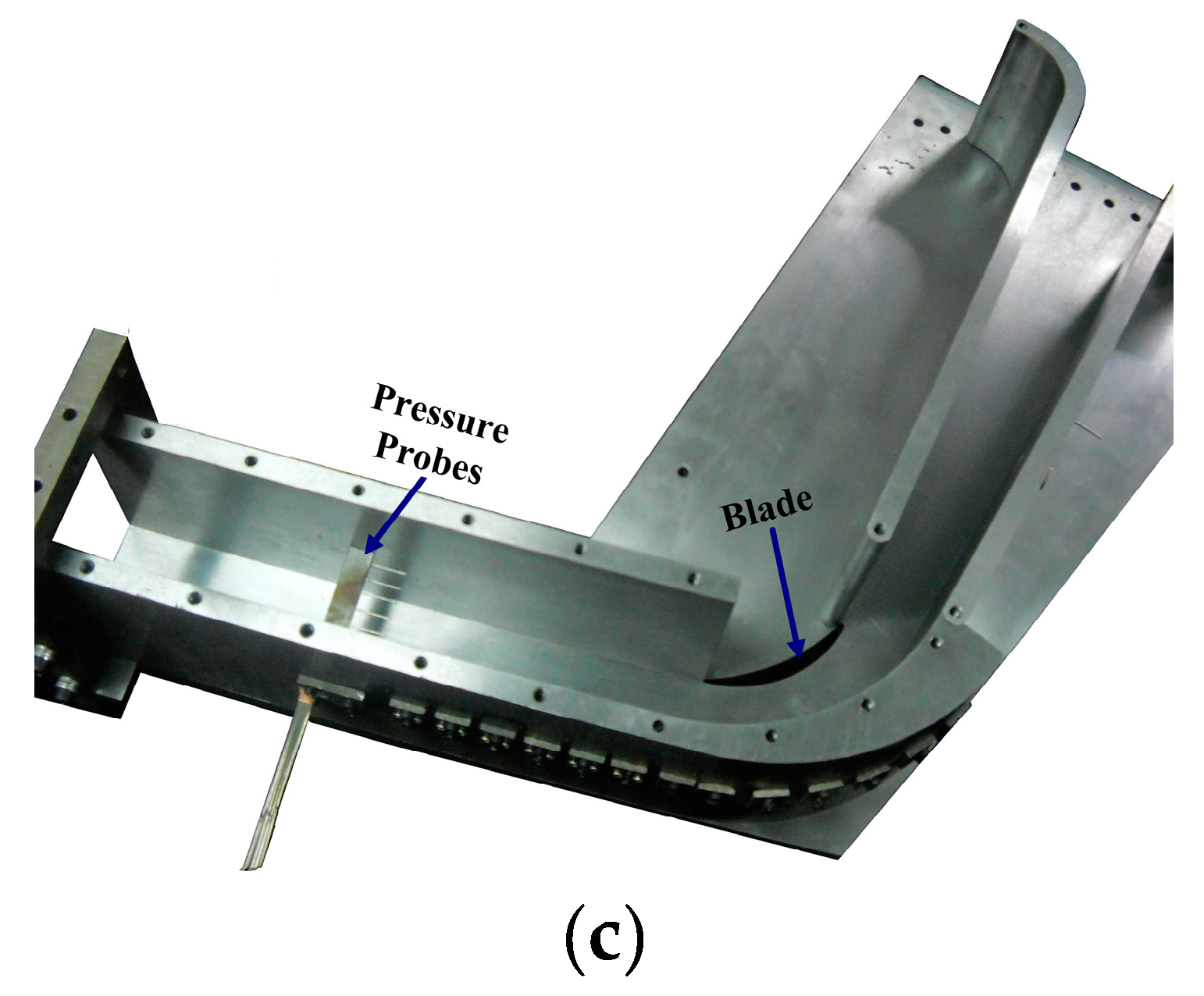
In addition, some experimental data are obtained to verify the simulated characteristics. The experimental and measuring devices are shown in Figure 1c. Moreover, the pulsed jet without external energy is used as the flow control device. The hollow rotating shaft is driven and controlled by a stepping motor to adjust the jet frequency. The time-averaged measurement parameters mainly include the total and static pressure of the inlet/outlet. The pressure probes are located at 50% of the blade height in the diffuser to avoid the three-dimensional effect to a feasible extent. Reference [19] provides additional details about the numerical simulation and experiment.
2.3. Definition of the Parameters in Pulsed Jet Flow Control
We initially define some important parameters to analyze the phenomena in unsteady flow control. In pulsed jet flow control, the definition of the reduced frequency (or non-dimensional frequency) is:
where is the pulsed jet frequency, and is the natural frequency of the uncontrolled flow field.
The momentum coefficient in pulsed jet flow control is defined as [1]:
where , , , and are the density, velocity, slot width, and period of the pulsed jet, respectively; and , , and are the characteristic density, velocity, and length, respectively (parameters at the inlet of the diffuser are used in this case). The momentum coefficient is usually used to evaluate the intensity of flow control.
The reduced jet location is defined as:
where is the location of the pulsed jet, is the location of the separation point, and is the chord length in the curved diffuser.
The non-dimensional parameters , , and are used to describe the frequency, intensity, and location of pulsed jet flow control, respectively. Furthermore, we need a parameter to evaluate the flow loss or control performance of the curved diffuser. Assuming that and are the total pressure at the inlet and at the outlet of the curved diffuser, the total pressure loss coefficient ω of the curved diffuser is defined as:
Subsequently, we can calculate the total pressure loss coefficients with and without pulsed jet control (denoted as and , respectively). Flow controls are aimed to reduce flow loss. Thus, we define the relative total pressure loss coefficient , which bridges the flow losses with and without control, as follows:
This parameter is used to evaluate the overall effect on the separation in the curved diffuser.
2.4. Unique Phenomena of Pulsed Jet Flow Control
2.4.1. Frequency-Dependent Effect
The frequency-dependent effect indicates that the flow control is relevant with the frequency of external excitation. This effect also exists in the pulsed flow separation control of a curved diffuser.
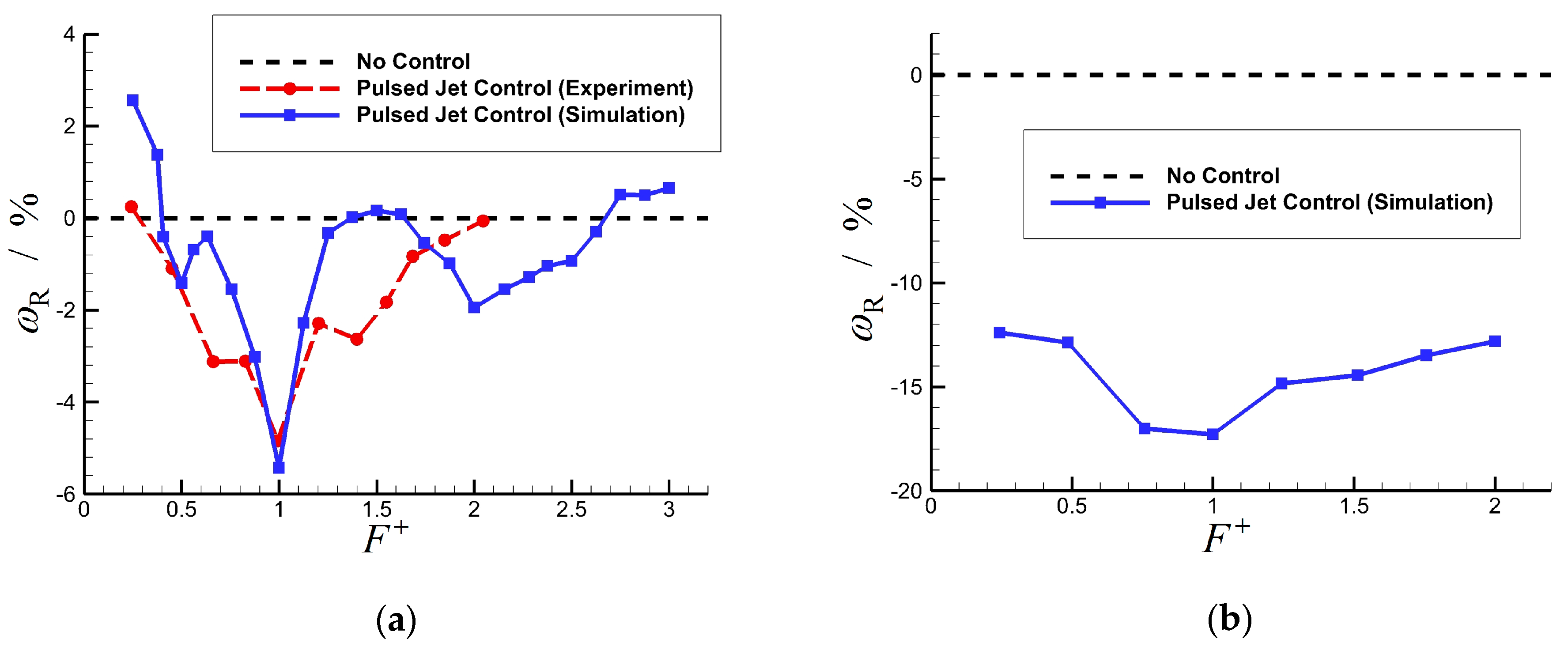
When , , and other parameters of the pulsed jet remain unchanged, the numerical simulation and experiment show that the relative total pressure loss coefficient varies with the pulsed jet frequency (Figure 2a). Notably, when , the total pressure loss coefficient is the lowest, whereas the flow control performance is the best. Moreover, when and , the numerical simulation shows that the relative total pressure loss coefficient is also the lowest when (Figure 2b). The frequency-dependent effect is reflected in both cases.
2.4.2. Threshold Effect
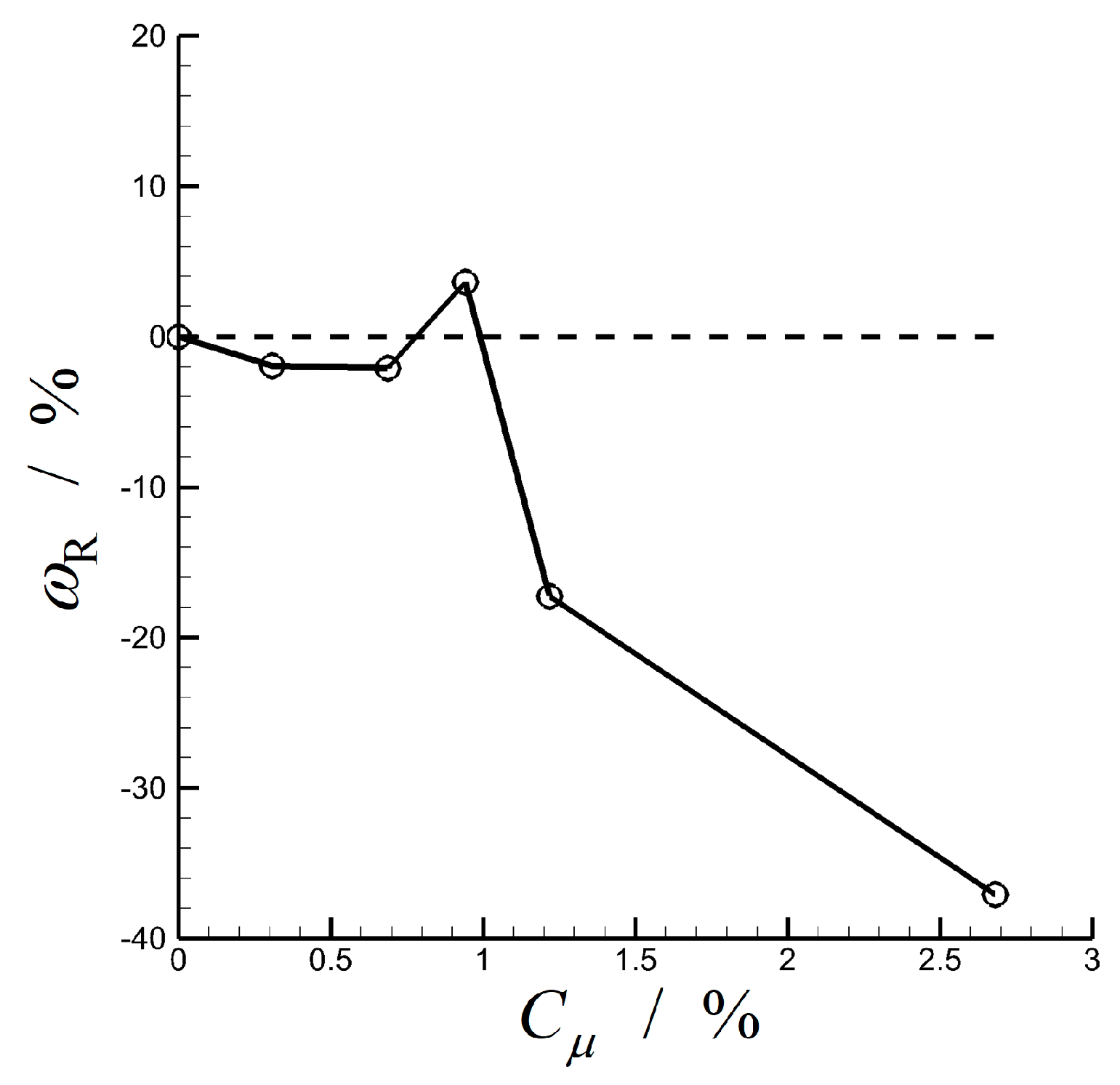
Threshold effect also exists in the pulse jet flow control of the curved diffuser. Figure 3 shows the relative total pressure loss coefficient () of the diffuser versus the momentum coefficient () of the pulsed jet when through numerical simulation. The threshold of momentum coefficient is approximately 1%. When the momentum coefficient is lower than this threshold, the total pressure loss coefficient does not considerably change. However, when the momentum coefficient is higher than this threshold, the total pressure loss coefficient decreases considerably with the momentum coefficient.
2.4.3. Location-dependent Effect
The numerical and experimental results show the relationship between the relative total pressure loss coefficient () of the curved diffuser and the reduced position of the pulsed jet () when , , and (Figure 4). The relative total pressure loss coefficient is the lowest when the pulsed jet is placed at the separation point, and the corresponding flow control performance is the best. As the position of the pulsed jet moves upstream or downstream of the separation point, the flow control performance decreases gradually.
2.4.4. Lock-on Effect
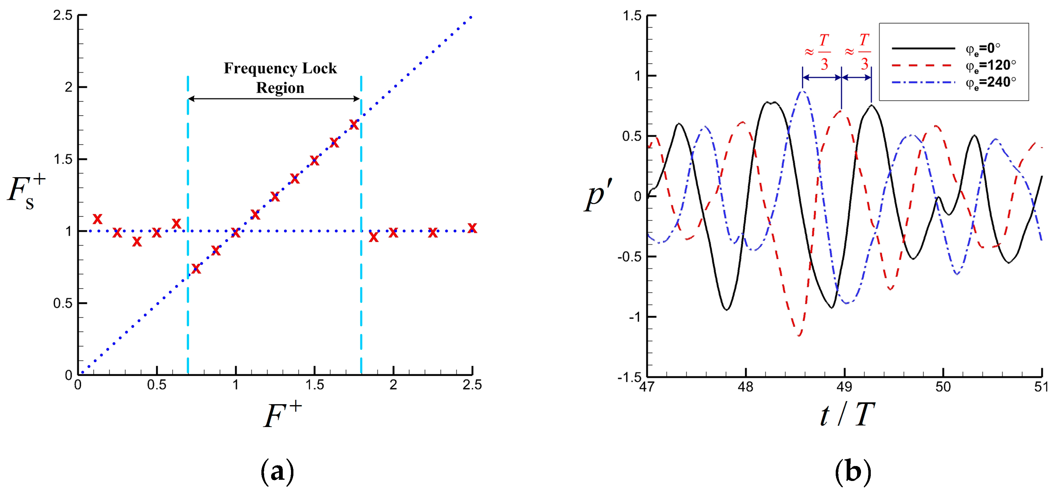
Lock-on effect reflects the relationship between the phase of external excitation and the control performance. Frequency and phase locking are the main characteristics of the lock-on effect [20,21]. Figure 5a shows the relationship between the reduced dominant frequency of the system (the flow field) (, where is the dominant frequency of static pressure at the monitoring points) versus the reduced frequency of the pulse jet . Frequency locking () only occurs near the region where , which is called the lock-on region. Inside this region, the control performance is also remarkable by coincidence. Outside the lock-on region, the main frequency of the system is the same (), which is approximately equal to that of the uncontrolled flow field.
Figure 5b shows the dimensionless fluctuating pressure (, where is the time-averaged static pressure) at the monitoring point that varies with time when and under different pulse jet phases . Although the amplitude of pressure changes in the actual flow, ( and are the phases of the pulsed jet and the system, respectively), which indicates the occurrence of phase locking.
The phenomenological analysis of pulse jet flow control in a curved diffuser exhibits frequency-dependent, threshold, position-dependent, and lock-on effects, which correspond to the frequency, intensity, position, and phase of the external excitation, respectively. These unique phenomena need further explanation to reveal the hidden control mechanism.
3. Theoretical Basis of Unsteady Flow Controls
Flow instability is the main factor in the generation of dominant coherent structures in flow separations, and the excited shear flow is the basis of unsteady flow control. Therefore, the basic theories of these two aspects are briefly introduced in this section. On the basis of these theories, the unique phenomena in unsteady flow separation control can be interpreted.
3.1. Linear and Weakly Nonlinear Stability Theory
3.1.1. Linear Stability Theory and O–S Equation
Some time-averaged velocity profiles are inherently unstable, and small disturbances in the environment can be amplified through flow instability and produce vortical structures. O–S equation is used to describe flow instability when the initial amplitude of disturbance is small. For two-dimensional parallel flow and given the x-direction velocity profile , the stream function of the initial disturbance can be expressed as a normal mode, shown as follows [19]:
where is conjugate with , (complex) is the wave number of perturbation wave, and (complex) is the angular frequency of perturbation wave. The non-dimensional O–S equation can be deduced by the linearization of N–S equation, as shown as follows [22]:
where is the dimensionless form of , (complex) is the phase velocity of perturbation wave, and is the Reynolds number. A series of discrete (or continuous, taking discrete as an example) eigenvalues and eigenfunctions can be obtained by solving this equation.
Equation (6) describes the stream function (as a special solution) of a perturbation wave and can be further expressed as follows:
where subscripts r and i represent the real and imaginary parts of a complex number, respectively; and are the temporal and spatial growth rates of the perturbation, respectively; and and are the angular frequency and wave number of the perturbation, respectively. In view of the temporal growth mode () and by linear superposition, the general solution at a certain Reynolds number is [22]
where is the initial amplitude of each mode. For a fixed point of coordinates x and y in the flow field, the following can be obtained:
where and represent the amplitude and phase, respectively. Similar forms can be obtained for other parameters in the flow field.
3.1.2. Weakly Nonlinear Stability Theory and S–L Equation
To make the O–S equation linear, a hypothesis of small perturbations was made, resulting in failure of describing nonlinear phenomenon, such as saturation of perturbation. However, the S–L equation is a weakly nonlinear model, which is used to model supercritical bifurcations and is able to deal with some typical nonlinear phenomena such as saturation of perturbation.
Equation (10) shows that in linear stability theory, the amplitude of perturbation increases exponentially, and the amplitude of a normal mode has the following relation:
Thus, the growth rate of perturbation consistently remains constant , and the perturbation increases infinitely with time, which is contrary to the actual physics. Only the time-averaged flow and the dominant normal modes of two-dimensional parallel flow are considered. Thus:
The nonlinear Reynolds stress term is neglected in linear stability theory, and is considered by an approximate method; hence, the following can be derived [15]:
where is the growth rate of perturbation in linear stability theory, and is the Landau constant. This equation is an S–L equation that can accurately describe the flow phenomena near the critical point. Equation (13) shows that when , , which means the disturbance amplitude will saturate due to the nonlinear effect.
For the spatial growth mode, the time-related and need to be replaced by space-related and in Equation (13), which yields:
Equation (14) can be used to describe the nonlinear spatial evolution of the dominant disturbance amplitude approximately.
3.2. Free Shear Flow Theory
3.2.1. Free Shear Flow without Excitation
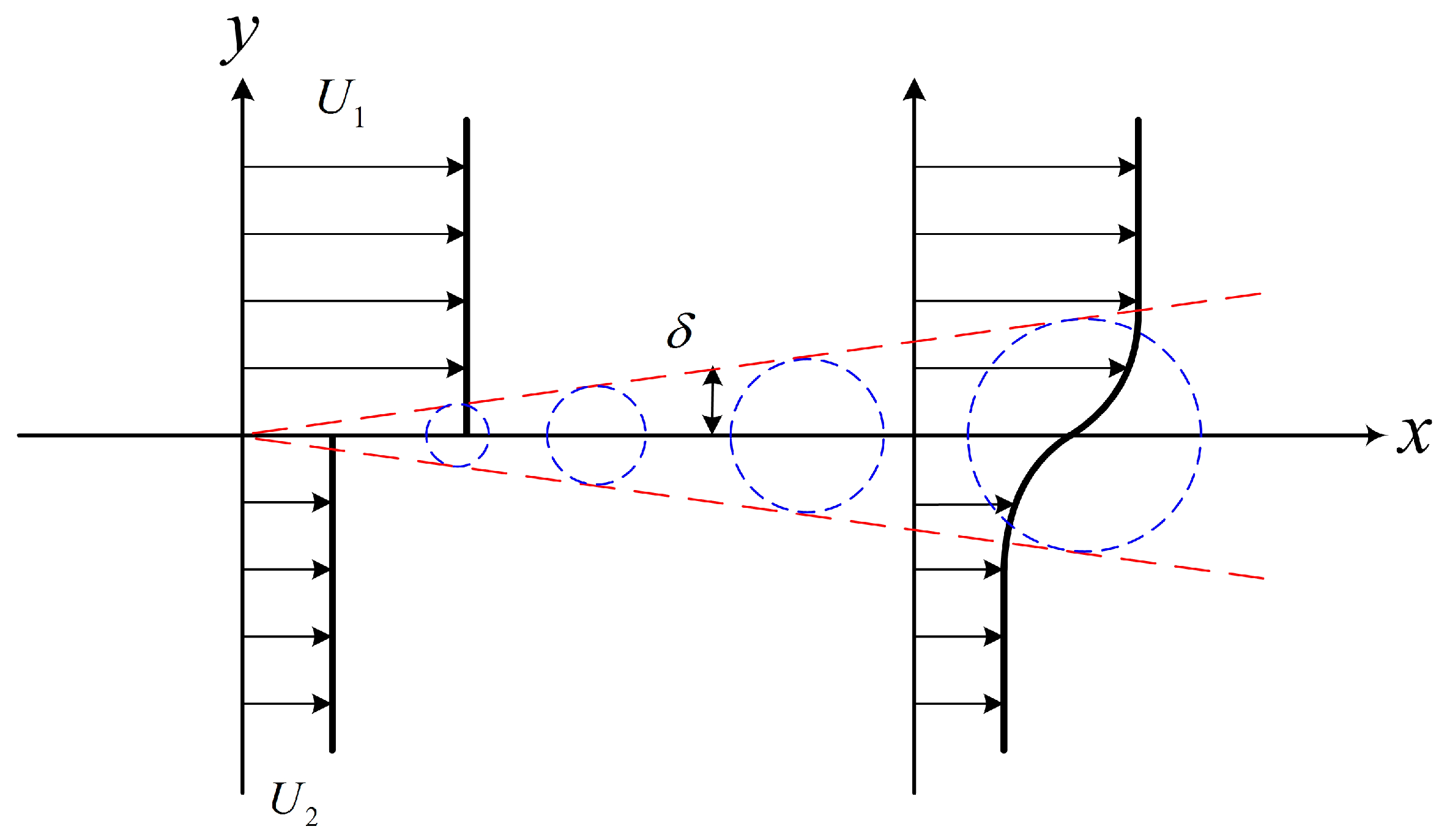
A free shear layer is composed of two parallel flows with different velocities and (the difference of density is not considered), as shown in Figure 6. Small disturbances in the environment will destabilize the shear layer, and vortical structures will roll up because the velocity profile is unstable. This unstable phenomenon is called K–H instability. Similar to the concept of boundary layer thickness, the shear layer thickness gradually increases downstream. Two other important parameters in the free shear layer are the characteristic velocity () and velocity ratio (). Moreover, the velocity profiles of the same shear flow at different streamwise locations are approximately similar, which indicates that:
On the basis of linear stability theory, an analytical relationship is observed between the non-dimensional growth rate and frequency of the piecewise linear free shear flow, that is, [23]
where is the non-dimensional growth rate of perturbation (), and is the non-dimensional angular frequency of perturbation (). Figure 7 shows the relationship between and . When is approximately 0.8 (denoted as ), reaches its maximum (denoted as ). The corresponding mode is the most unstable in the free shear flow (with a maximum growth rate). This mode will then develop rapidly, thereby suppressing other modes with a smaller growth rate, developing into the dominant mode, and generating into large-scale vortices. at different stream-wise positions are the same due to the similarity of velocity profiles of the shear layer. However, with the stream-wise development of the shear layer and the increase of , the dimensional frequency of the dominant mode () decreases gradually. Therefore, the low-frequency vortices will gradually dominate downstream in the shear layer, and this process is usually accomplished by the merging of small high-frequency vortices into large low-frequency ones.
The laminar free shear flow is easy to develop into turbulence due to flow instability. For turbulent free shear layers, theoretical and experimental studies show that the thickness of the shear layer has the following relationship [17]:
where is a constant. Therefore, the thickness of turbulent free shear layer develops linearly along the stream-wise direction. Moreover, the most unstable frequency at different stream-wise positions in turbulent free shear flow has the following relationship:
That is, the characteristic frequency of turbulent free shear flow is proportional to the average velocity and inversely proportional to the velocity ratio and stream-wise distance.
3.2.2. Turbulent Free Shear Flow under Periodic Excitation
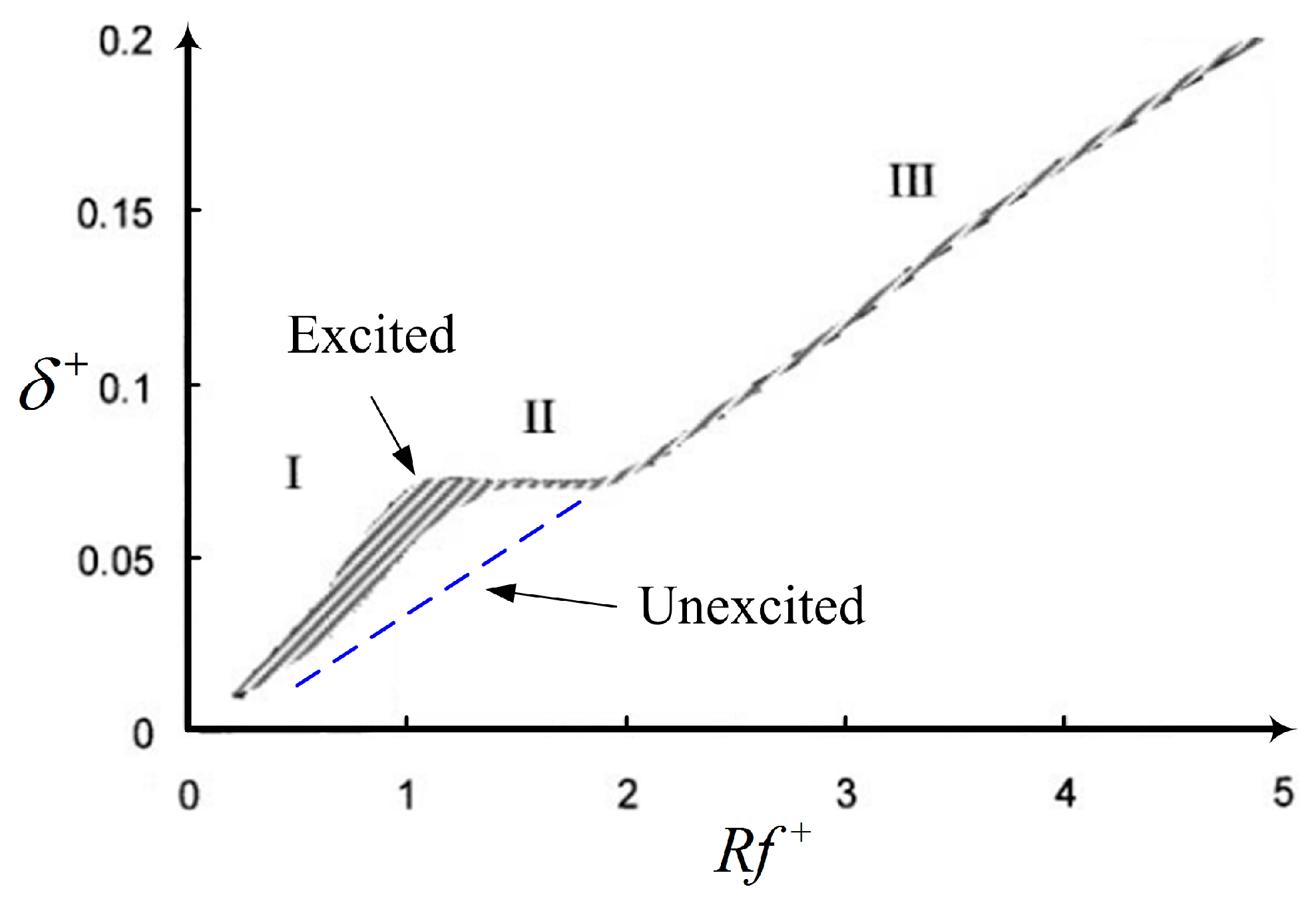
Turbulent free shear flow under periodic excitation has different flow characteristics from that without excitation; thus, it becomes the theoretical basis of unsteady flow control. The streamwise development of the momentum thickness of turbulent free shear flow under periodic excitation is shown in Figure 8, in which the excitation is located at the beginning of the shear flow. In this figure, is defined as the nondimensional momentum thickness, and ; is another nondimensional parameter, and , where is the excitation frequency [1]. As shown in Figure 8, the development of the excited turbulent free shear flow can be divided into three stages as follows (see References [24] and [25] for more information). of the first stage is between 0 and 1, and the momentum thickness of the shear layer increases rapidly due to K–H instability with external excitation. of the second stage is approximately between 1 and 2, and the growth of perturbation is saturated or neutrally stable. of the third stage is more than 2, and the momentum thickness of the shear layer increases linearly, similar to that without external excitation. The comparison of the linear development of the turbulent free shear flow without external excitation (Figure 8) shows that the main difference between the two situations is caused by the first two stages influenced by excitation. Hence, external excitation can change the development of momentum thickness and corresponding momentum transfer between high- and low-velocity fluids.
In sum, under the influence of external excitation, the development of vortices and momentum thickness at the first and second stages is determined by external excitation, and the dominant frequency is equal to the excitation frequency. The third stage is characterized by the pairing and merging of vortices, that is, the dominant frequency decreases downstream; whereas the development of momentum thickness is not controlled by external excitation, and its behavior is similar to what is described in Equation (17). Further analysis of the second stage shows that and . Thus, and (subscript 2 denotes the second stage), which indicates that a higher frequency of external excitation results in faster occurrence of saturation (neutrally stable state) and a smaller corresponding saturated momentum thickness.
4. Interpretation of Unique Phenomena and Mechanism in Unsteady Separation Flow Control
Unique phenomena are observed in unsteady flow separation control, such as frequency-dependent, threshold, position-dependent, and lock-on effects. These phenomena can be explained by the theories of flow stability and excited free shear flow, from which the mechanism of unsteady flow control can be inferred.
4.1. Interpretation of Frequency-Dependent Effect Based on Excited Free Shear Flow Theory
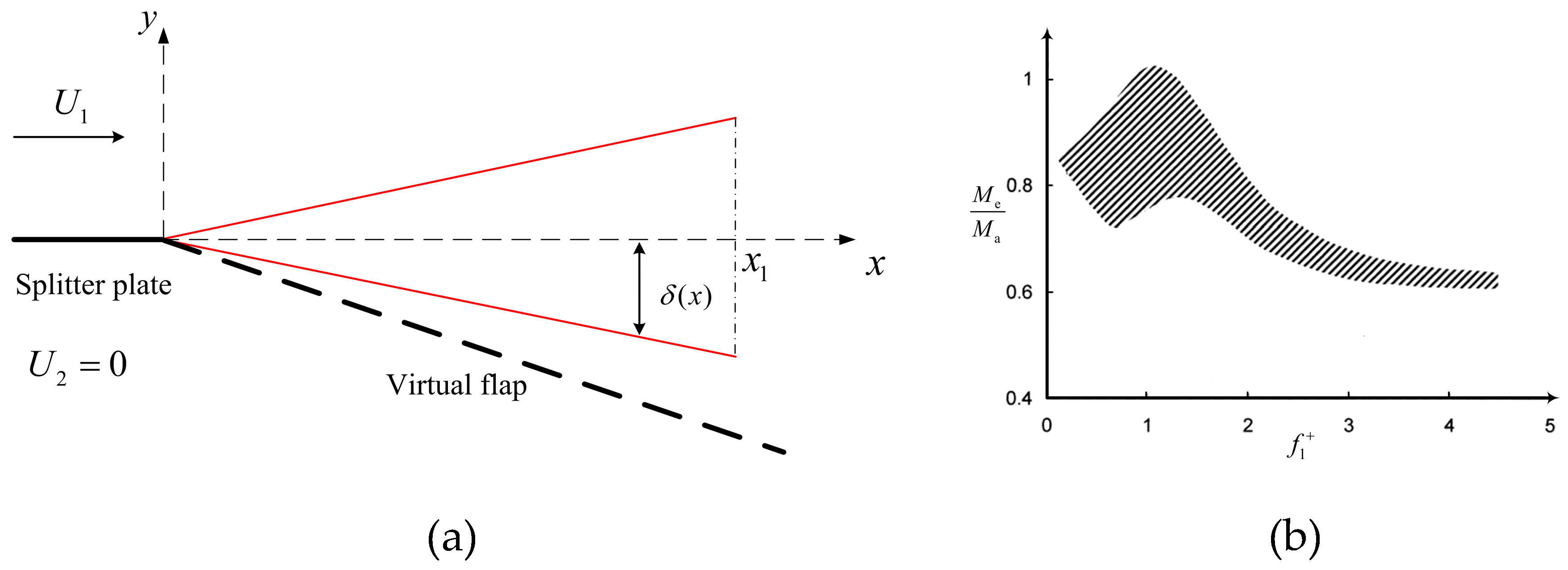
The momentum thickness of free shear layer measures the momentum transfer between high- and low-velocity fluids. Figure 9a shows that given in a free shear flow, an imaginary plate is assumed to be inserted into the stationary lower half plane of fluid to form a virtual wall. Without considering viscosity and instability, a stagnant area formed between the virtual plate and the x-axis can be approximately considered a “separation zone,” whereas the fluid of the upper half plane is the mainstream. When the coherent structures and the corresponding momentum thickness in the shear layer develop along the x-direction, they are unaffected by the virtual plate (“separation” will not “reattach”). Then, half of the integral of the momentum thickness along the x-axis reflects the influence area of the coherent structures of the shear layer on the separation zone. To reflect the proportion of momentum transferred from mainstream into the separation zone by shear layer, the entrainment ratio (the ratio of the fluid mass gaining momentum in the separation zone to the total mass available ) is defined as follows [1]:
where , , and . The development curve of the entrainment ratio can be obtained through the relationship in Figure 8, as shown in Figure 9b [1]. The entrainment ratio reaches its largest when . Under this situation, the momentum transferred from the mainstream to the separation zone is the largest by changing the development characteristics of the shear flow. Notably, the shear flow is now at the second stage (neutrally stable stage) in Figure 8. On the basis of the definition of , , which indicates the frequency dependence of the unsteady excitation.
The momentum thickness or the scale of coherent structures can increase ceaselessly because no global characteristic scale is observed for free shear flow; this condition is inconsistent with common engineering applications of a determined characteristic scale. Thus, the shear layers with global characteristic scale is further analyzed, as shown in Figure 10. From the figure, the virtual plate only restricts the momentum thickness of the shear layer to not exceed (twice the distance between the virtual plate and the x-axis). Hence, on the basis of Equation (18), the natural frequency at the end of the shear flow is:
The development of momentum thickness of the shear layer under three typical excitation frequencies is illustrated in Figure 10. When , the shear layer saturates fast, and the saturated momentum thickness is less than ; when , the saturated momentum thickness is equal to ; when , the shear layer is not saturated spontaneously but is limited to at the end of its development. In this figure, the area wrapped by the development curve of momentum thickness and the x-axis can reflect the momentum transfer from the mainstream to the separation zone. The momentum transfer when is less than that when . Moreover, from the analysis of Equation (19) and in the region that , only the situation that can make the shear layer end up at the second stage. Therefore, when the excitation frequency is equal to the natural frequency that corresponds to the characteristic scale of the shear flow, the most momentum transfer can be reached and the most effective “suppression’ on “separation” is achieved from the perspective of time-averaged flow. This interpretation of frequency-dependent effect is based on shear flow theory. The optimum excitation frequency should be selected as the natural frequency (vortex shedding frequency) of the uncontrolled flow field in pulsed jet flow control.
4.2. Interpretation of Threshold and Lock-On Effects Based on Linear Stability Theory
The precondition for effective unsteady flow control is that the excitation has sufficient influence on or even dominates the flow field. Within a certain range of parameters (e.g., the excitation intensity is greater than a certain threshold (, and is the threshold momentum coefficient) or its frequency near the natural frequency ), the unsteady separated flow can be synchronized with or locked by the external excitation. This phenomenon can be explained by linear stability theory. Although the nonlinear characteristics cannot be described, linear stability theory can accurately predict the dominant frequency of an unstable flow without external excitation, which is due to the fact that the vortical structures in the nonlinear stage are mainly developed from the dominant perturbation wave in the linear stage. On the basis of Equation (13), the sensitivity or growth rate of perturbation decreases with the increase in disturbance amplitude; thus, the flow field is the most sensitive at its initial development stage of perturbation wave and is the most effective stage for external excitation.
For unstable flows (e.g., separated flows) under external excitation, the dominant frequency of large-scale coherent structures is assumed to be determined by the dominant mode, which is competed by environmental white noise perturbations and external excitations in the linearly developing stage. And the dominant saturated mode then develops nonlinearly to be the dominant mode. Thus, the main characteristics of fully developed perturbation waves can be roughly understood by analyzing its linear stage. In the linear stage, given the discrete form of the characteristic functions, the stream function in Equation (10) can be replaced by any parameter of the flow field (pressure and velocity) and the external excitation term (denoted by the subscript e) is added. Thus:
where , , , and are the amplitude, growth rate, angular frequency, and initial phase of external excitation, respectively. For simplification, the initial amplitude of white noise perturbation of each frequency is considered . For the perturbation growth rate, is stipulated; hence, is the dominant or natural frequency of flow without excitation (the same to ), and its corresponding growth rate is . The value of is random due to the characteristics of white noise. Several situations are discussed as follows.
a. Under the situation of no external excitation, the unstable flow is still in the linear growth stage after a period of time (assuming the critical time between linear and nonlinear stage is ). Exponential growth in the linear stage will soon widen the gap between the perturbation amplitudes of different growth rates; thus, the perturbation frequency of the maximum growth rate will quickly dominate. Hence, when :
where the dominant frequency of the flow field is , and the corresponding phase is .
b. External excitation is added, and . When , the expression of is the same with Equation (22) because the external excitation will be submerged in environmental noise and does not result in effective control. This result implies that the intensity of external excitation needs to reach a certain threshold to achieve effective control; this phenomenon is called threshold effect.
c. External excitation is added, and . When and , the expression of is presented in Equation (22). The external excitation fails to function due to the low growth rate of the external frequency. However, when and :
Under this situation, if , then , and the dominant perturbation wave will saturate faster. If , then the original perturbation wave will be counteracted, and the perturbation wave that corresponds to will dominate. However, in the free shear flow, the frequency of the perturbation wave varies continuously (Figure 7). Thus, and , which indicate that the expression of tends to approach Equation (22). The original dominant perturbation wave is suppressed; thus, the second-order perturbation wave develops into the dominant one, which is similar to the original. Notably, the guarantee of or needs the aid of closed-loop control, whereas the relationship between and in open-loop control is random.
d. External excitation is added, and . On the basis of Equation (21), when and :
Under this situation, the main flow frequency is still the dominant frequency without excitation; however, its phase is locked to by the external excitation, and the saturation of the perturbation wave is faster, which is similar to the resonance phenomenon in the linear vibration theory. If and , then the expression of still tends to Equation (22) when due to the low growth rate of the excitation frequency. Then, the external excitation has no considerable control effect, which is different from the linear vibration theory. However, if and , then the growth rate of the excitation frequency is sufficiently high. Thus, when :
Similar to the resonance in linear vibration theory, the main frequency and phase of fluid system are determined by external excitation, which is called the frequency- and phase-lock or lock-on phenomenon. Thus, although , lock-on will occur if the growth rate of external excitation is sufficiently large, which is why a lock-on region exists in Figure 5a. The threshold and lock-on effects are interpreted in this section based on linear stability theory.
4.3. Interpretation of Location-Dependent Effect Based on Nonlinear Stability Theory
Unsteady flow control has a position-dependent effect; that is, the flow control performance is usually the best when the control is applied near the separation point. This phenomenon can be explained by the theory of nonlinear flow stability. For a typical two-dimensional flow separation, the separation point can be approximated as the starting point of the K–H instability, such that the flow separation can be idealized as the shear flow illustrated in Figure 9a from the view of stability analysis. The flow upstream the separation point is similar to the boundary layer flow on a flat plate. K–H instability does not exist, and the spatial growth rate of perturbation is less than zero. The flow downstream the separation point is similar to the shear flow. K–H instability exists, and the spatial growth rate of perturbation is greater than zero. In linear stability theory, the growth rate of perturbation ( in temporal mode or in spatial mode) reflects the receptivity or sensitivity of the flow field to a certain mode, and the perturbation with the largest growth rate can quickly form the dominant mode in the flow field. The actual flow field is affected by nonlinearity; thus, the growth rate of perturbation decreases gradually with the increase in perturbation amplitude. The sensitivity of flow field to external perturbation decreases accordingly. On the basis of the approximate expression of spatial development of perturbation amplitude in weakly nonlinear stability theory (Equation (14)), the spatial growth rate of disturbance amplitude is shown as follows (in non-dimensional form):
where is the initial perturbation amplitude. When , and , the spatial growth rate of perturbation amplitude is illustrated in Figure 11. In this figure, the abscissa is the distance , the ordinate is the spatial growth rate , and the separation point (the starting point of instability) is located at . Upstream the separation point of , , and the blue dotted line of is used to indicate this point. At the separation point of , ; hence, the growth rate of perturbation reaches its maximum. Downstream the separation point of , , and decreases gradually with the increase of until it approaches zero, as shown in the red solid line in Figure 11. In this simplified flow diagram, the flow field has the strongest sensitivity to external perturbation in the vicinity of the separation point; hence, the excitation placed near here tends to play an effective role in flow control. If the excitation is placed far away from the separation point, then the excitation intensity received by the flow near the separation point (nearby which is the most sensitive flow field) is inevitably lower than the original intensity of the excitation. Thus, the threshold effect jeopardizes the control performance.
These analyses briefly interpret the frequency-dependent, threshold, lock-on, and position dependent phenomena in unsteady flow separation control. Moreover, the mechanism of unsteady flow separation control will be discussed in the following section.
4.4. Interpretation of Unsteady Flow Separation Control Mechanism
The four phenomena in unsteady flow control provide clues of unsteady flow control mechanisms. Frequency- and location-dependent effects are closely related to the receptivity or sensitivity of flow separation. As interpreted previously, location-dependent effect occurs because the separation point is the starting point of K–H instability, and the flow field has the most sensitivity nearby. Moreover, frequency-dependent effect indicates that the optimum excitation frequency is the natural frequency of the uncontrolled flow. Notably, natural frequency happens to be the most unstable. Thus, the optimum excitation frequency and location correspond to the most sensitive frequency and location. The concurrence of this phenomenon is not just a coincidence, and there lie profound mechanisms behind them. Unsteady flow control has the advantage of using minimal control energy to achieve the same performance compared with steady control. Thus, the use of sensitivity is an economic way to amplify the effect of external excitation with minimal energy. Hence, the first mechanism of unsteady flow separation control is to utilize flow instability and excite the most unstable or sensitive mode in the flow.
Another mechanism functions when the external excitation interacts with the vortical structures in flow separation. According to threshold and lock-on effects, when the intensity and frequency of the excitation are proper, the dominant vortical structures in flow separation will be synchronized or locked with external excitation. The lock-on parameters coincide with those of effective control. Thus, although the optimum frequency and location of excitation are selected, effective flow control may not be achieved. At this time, the excitation intensity matters, and only if lock-on occurs, can the flow field be entirely manipulated by external excitation, which results in effective control performance. This condition is the second mechanism of unsteady flow control related to the lock-on.
Exciting the most unstable mode is not the final step. After the most unstable mode of perturbation is excited externally, the mode subsequently forms into vortical structures. The aforementioned analysis of frequency-dependent effect and entrainment ratio shows that proper external excitation will promote the saturation of vortical structures at appropriate positions while maximizing the momentum transfer from the mainstream to the separation zone. The momentum transfer will then suppress the time-averaged flow separation. This condition is the third mechanism of unsteady flow separation control, which is related to saturation and momentum transfer under external excitation.
Therefore, an effective unsteady flow control initially uses flow instability (sensitivity) to amplify itself. The flow field is then locked with its own pace (frequency and phase), the momentum is transferred from the mainstream to the separation zone through the excited coherent structures (excited modes), and the time-averaged flow separation is finally suppressed.
5. Conclusions
Unsteady flow controls are effective for suppressing flow separations. In this study, unique phenomena, namely, frequency-dependent, threshold, location-dependent, and lock-on effects, are discussed and interpreted. We initially present the results by numerical simulation and experiment of a separated curved diffuser using pulsed jet flow control to show these four phenomena. Then, to elucidate the phenomena and mechanism in unsteady flow separation control, we introduce the basis of unsteady flow control, which are the theories of flow instability and free shear flow. Finally, using these theories, the four phenomena of unsteady flow control are interpreted, as well as the hidden mechanisms. The main conclusions are obtained as follows:
- (1)
- Four phenomena, namely, frequency-dependent, threshold, position-dependent, and lock-on effects, lie in unsteady flow control. Frequency-dependent effect indicates that when the external excitation frequency is near a certain value (usually the natural frequency of the flow), the control performance is the best. Threshold effect implies that only when the intensity of external excitation reaches a certain value or more can a significant control effect be achieved. Location-dependent effect refers to the fact that the optimal location of external excitation is generally at or near the separation point. Lock-on effect includes phase- and frequency-lock; it indicates that when the control parameters are proper, the flow field will be locked to the external excitation. These four unique phenomena are found in the separated curved diffuser with pulsed jet flow control.
- (2)
- The basis of unsteady flow control includes stability and free shear flow theories. In this study, the stability theory of O–S and S–L equations and the unexcited and excited free shear flow theories are introduced. Moreover, the interpretations of the four phenomena are all based on these theories.
- (3)
- Frequency-dependent effect is interpreted on the basis of excited free shear flow theory. The momentum transferred through coherent structures in shear flow or entrainment ratio is greatly dependent on the excitation frequency because the external excitation can determine when and where neutral stability will occur. On the basis of an idealized flow model (with characteristic scale) that bridges the shear flow and flow separation, the optimum excitation frequency happens to be the natural frequency without control, which interprets the frequency-dependent effect found in the unsteady flow control.
- (4)
- Threshold and lock-on effects are interpreted on the basis of linear stability theory. For unstable flows under external excitation, the dominant frequency of large-scale coherent structures is assumed to be determined by the dominant mode competed by environmental white noise perturbations and external excitations in the linear stage. Discussion on the linear stage indicates that the flow will be locked to the excitation only when excitation intensity is sufficiently large; otherwise, the excitation will be submerged in environmental noise. The excitation frequency for lock-on is specified because its corresponding growth rate must be sufficiently large to exceed a naturally developed dominant mode.
- (5)
- Location-dependent effect is interpreted on the basis of weakly nonlinear stability theory. The separation point of a typical two-dimensional flow separation can be approximated as the starting point of the K–H instability, such that the flow separation can be idealized as the shear flow from the view of stability analysis. On the basis of weakly nonlinear stability theory, the flow field has the strongest sensitivity to external perturbation in the vicinity of the separation point. Thus, the excitation placed near it tends to result in effective flow control.
- (6)
- The four phenomena in unsteady flow control show clues of the control mechanism. In this study, an effective unsteady flow control initially uses flow instability (sensitivity) to amplify itself, lock the flow field with its own pace (frequency and phase), transfer the momentum from the mainstream to the separation zone through the excited coherent structures (excited modes), and finally suppress the time-averaged flow separation.
Author Contributions
W.L. performed the theoretical analyses and wrote the manuscript; G.H. proposed the research route and method; J.W. contributed to simulation and data analyses; Y.Y. contributed to manuscript preparation.
Funding
This research was funded by the National Basic Research Program of China (No. 2014CB239602) and the National Natural Science Foundation of China (No. 51176072).
Acknowledgments
The authors wish to express their gratitude to Jiangsu Province Key Laboratory of Aerospace Power System (affiliated with the College of Energy and Power Engineering, Nanjing University of Aeronautics and Astronautics) for technical support. The team members of College of Energy and Power Engineering of Nanjing University of Aeronautics and Astronautics are also gratefully acknowledged for their cooperation.
Conflicts of Interest
The authors declare no conflicts of interest.
References
- Greenblatt, D.; Wygnanski, I.J. The control of flow separation by periodic excitation. Prog. Aerosp. Sci. 2000, 36, 487–545. [Google Scholar] [CrossRef]
- Collis, S.S.; Joslin, R.D.; Seifert, A.; Theofilis, V. Issues in active flow control: Theory, control, simulation, and experiment. Prog. Aerosp. Sci. 2004, 40, 237–289. [Google Scholar] [CrossRef]
- Nishioka, M.; Asai, M.; Yoshida, S. Control of flow separation by acoustic excitation. AIAA J. 1990, 28, 1909–1915. [Google Scholar] [CrossRef]
- Glezer, A.; Amitay, M. Synthetic jets. Ann. Rev. Fluid Mech. 2002, 34, 503–529. [Google Scholar] [CrossRef]
- Hecklau, M.; Wiederhold, O.; Zander, V.; King, R.; Nitsche, W.; Swoboda, M. Active separation control with pulsed jets in a critically loaded compressor cascade. AIAA J. 2011, 49, 1729–1739. [Google Scholar] [CrossRef]
- Wu, X.; Wu, J.; Wu, J. Streaming effect of wall oscillation to boundary layer separation. In Proceedings of the AIAA 29th Aerospace Science Meeting, Reno, NV, USA, 7–10 January 1991. [Google Scholar]
- Wu, C.J.; Wang, L.; Wu, J.Z. Suppression of the Von Karman Vortex street behind a circular cylinder by a traveling wave generated by a flexible surface. J. Fluid Mech. 2007, 574, 365–391. [Google Scholar] [CrossRef]
- Singhal, A.; Castañeda, D.; Webb, N.; Samimy, M. Unsteady Flow Separation Control over a NACA 0015 using NS-DBD Plasma Actuators. In Proceedings of the 55th AIAA Aerospace Sciences Meeting, AIAA SciTech Forum, AIAA 2017–1687, Grapevine, TX, USA, 9–13 January 2017. [Google Scholar]
- Seifert, A.; Darabi, A.; Wygnanski, I. Delay of airfoil stall by periodic excitation. J. Aircr. 1996, 33, 691–698. [Google Scholar] [CrossRef]
- Hsiao, F.B.; Shyu, R.N.; Chang, R.C. High angle of attack airfoil performance improvement by internal acoustic excitation. AIAA J. 1994, 32, 655–662. [Google Scholar] [CrossRef]
- Chen, J.; Lu, W.; Huang, G.; Zhu, J.; Wang, J. Research on pulsed jet flow control without external energy in a blade cascade. Energies 2017, 10, 2004. [Google Scholar] [CrossRef]
- Greenblatt, D.; Nishri, B.; Darabi, A.; Wygnanski, I. Some Factors Affecting Stall Control with Particular Emphasis on Dynamic Stall. In Proceedings of the AIAA 30th Fluid Dynamics Conference, Norfolk, VA, USA, 28 June–1 July 1999. [Google Scholar]
- Wygnanski, I. The Variables Affecting the Control of Separation by Periodic Excitation. In Proceedings of the AIAA 2nd Flow Control Conference, Portland, OR, USA, 28 June–1 July 2004. [Google Scholar]
- Skamnakis, D.; Papailiou, K. Flow stability analysis and excitation using pulsating jets. C. R. Mécanique 2005, 333, 628–635. [Google Scholar] [CrossRef]
- Stuart, J.T. On the non-linear mechanics of hydrodynamic stability. J. Fluid Mech. 1958, 4, 1–21. [Google Scholar] [CrossRef]
- Gursul, I.; Cleaver, D.J.; Wang, Z. Control of low Reynolds number flows by means of fluid-structure interactions. Prog. Aerosp. Sci. 2014, 64, 17–55. [Google Scholar] [CrossRef]
- Dimotakis, P. Turbulent free shear layer mixing. In Proceedings of the AIAA 27th Aerospace Sciences Meeting, Reno, NV, USA, 9–12 January 1989. [Google Scholar]
- Wygnanski, I.J.; Petersen, R.A. Coherent motion in excited free shear flows. AIAA J. 1987, 25, 201–213. [Google Scholar] [CrossRef]
- Huang, G.; Lu, W.; Zhu, J.; Fu, X.; Wang, J. A nonlinear dynamic model for unsteady separated flow control and its mechanism analysis. J. Fluid Mech. 2017, 826, 942–974. [Google Scholar] [CrossRef]
- Barbi, C.; Favier, D.P.; Maresca, C.A.; Telionis, D.P. Vortex shedding and lock-on of a circular cylinder in oscillatory flow. J. Fluid Mech. 2006, 170, 527–544. [Google Scholar] [CrossRef]
- Konstantinidis, E.; Bouris, D. Vortex synchronization in the cylinder wake due to harmonic and non-harmonic perturbations. J. Fluid Mech. 2016, 804, 248–277. [Google Scholar] [CrossRef]
- Grosch, C.E.; Salwen, H. The continuous spectrum of the Orr–Sommerfeld equation. Part 1: The spectrum and the eigenfunctions. J. Fluid Mech. 1978, 87, 33–54. [Google Scholar] [CrossRef]
- Herrmann, M. A Eulerian level set/vortex sheet method for two-phase interface dynamics. J. Comput. Phys. 2005, 203, 539–571. [Google Scholar] [CrossRef]
- Oster, D.; Wygnanski, I.J. The forced mixing layer between parallel streams. J. Fluid Mech. 1982, 23, 91–130. [Google Scholar] [CrossRef]
- Parezanović, V.; Laurentie, J.C.; Fourment, C.; Delville, J. Mixing layer manipulation experiment. Flow Turbul. Combust. 2015, 94, 155–173. [Google Scholar] [CrossRef]
Figure 1.
Diagram of the (a) curved diffuser and (b) pulsed jet flow control device; (c) experimental devices.
Figure 1.
Diagram of the (a) curved diffuser and (b) pulsed jet flow control device; (c) experimental devices.
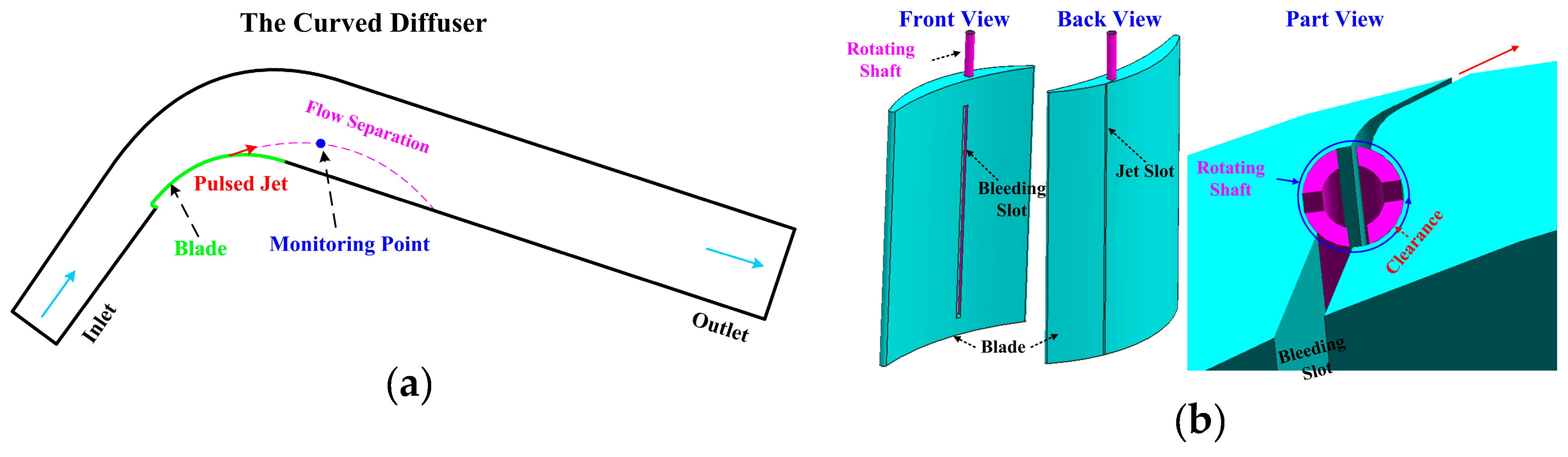

Figure 2.
Relative total pressure loss coefficient () of the curved diffuser versus reduced pulsed jet frequency (): (a) , ; (b) , .
Figure 2.
Relative total pressure loss coefficient () of the curved diffuser versus reduced pulsed jet frequency (): (a) , ; (b) , .

Figure 3.
Relative total pressure loss coefficient () of the curved diffuser versus momentum coefficient () of the pulsed jet ( and ).
Figure 3.
Relative total pressure loss coefficient () of the curved diffuser versus momentum coefficient () of the pulsed jet ( and ).

Figure 4.
Relative total pressure loss coefficient () of the curved diffuser versus reduced position () of the pulsed jet (when , , and ).
Figure 4.
Relative total pressure loss coefficient () of the curved diffuser versus reduced position () of the pulsed jet (when , , and ).
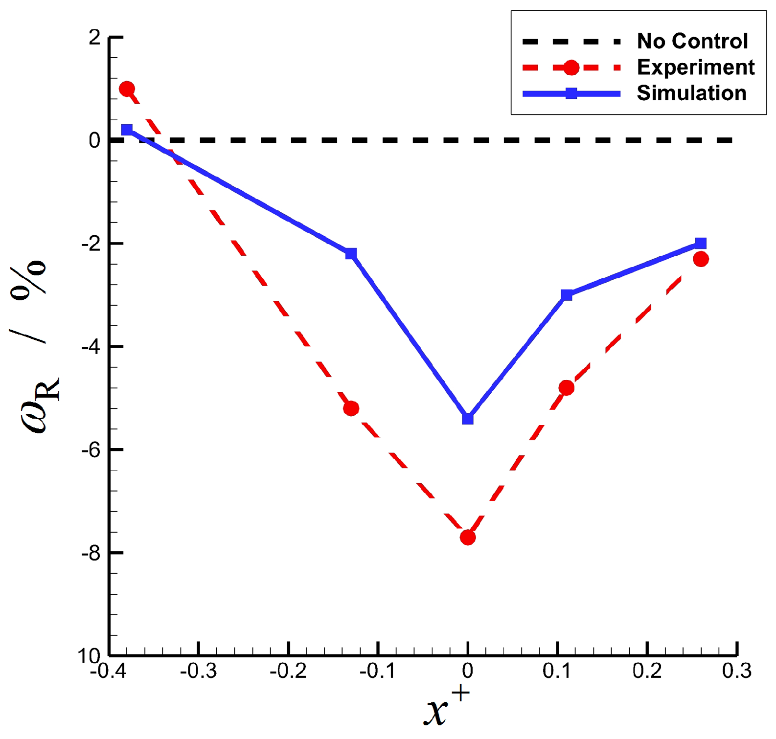
Figure 5.
Lock-on effect in the curved diffuser with pulsed jet flow control: (a) Frequency locking (reduced dominant frequency of the system versus reduced frequency of pulse jet ); (b) phase locking ( with different values of ).
Figure 5.
Lock-on effect in the curved diffuser with pulsed jet flow control: (a) Frequency locking (reduced dominant frequency of the system versus reduced frequency of pulse jet ); (b) phase locking ( with different values of ).

Figure 6.
Schematic representation of free shear flow development.

Figure 7.
Growth rate of different frequencies in free shear flow by linear stability theory.
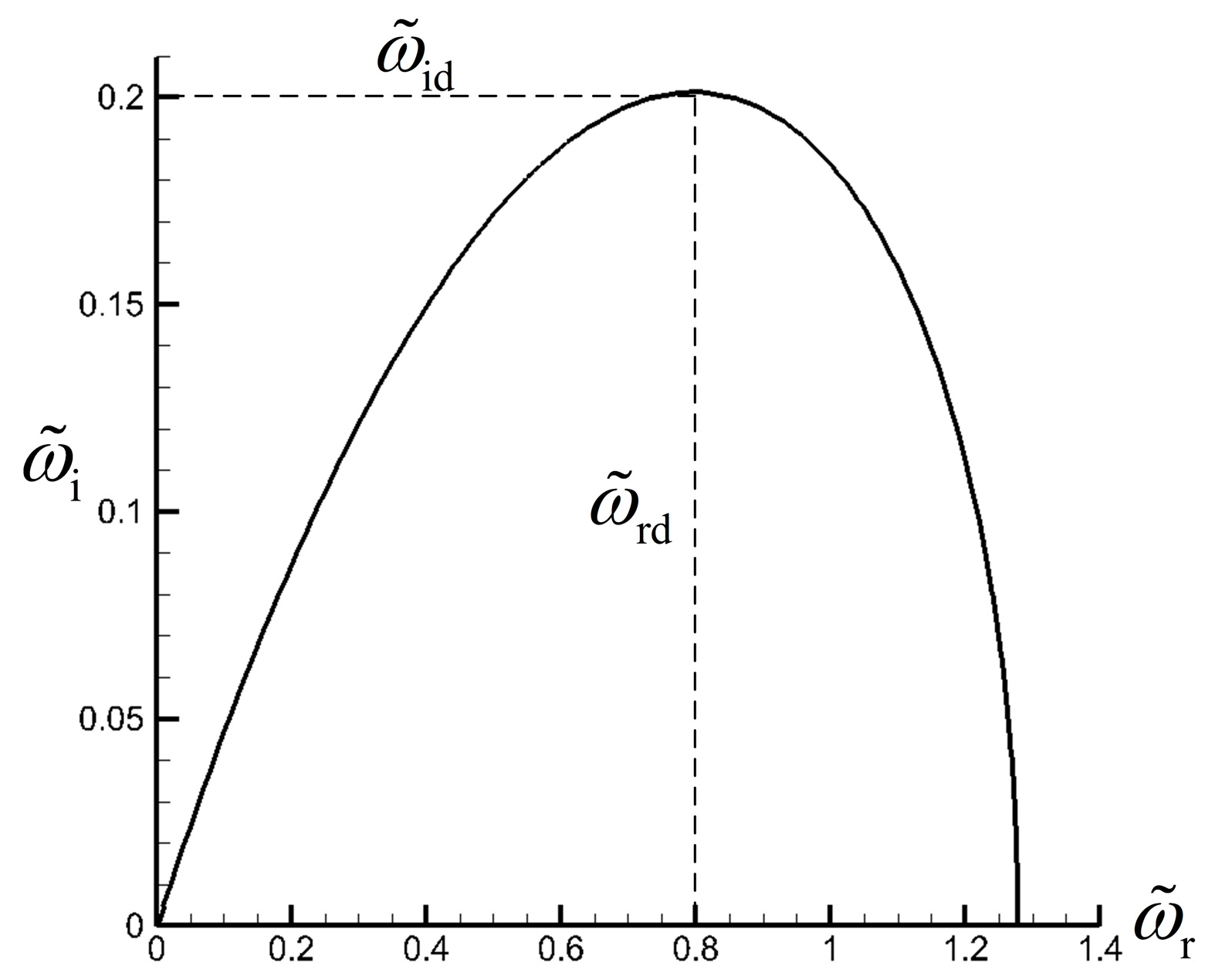
Figure 8.
Momentum Thickness Development of Excited Turbulent Free Shear Flows (Referring to [1]).
Figure 8.
Momentum Thickness Development of Excited Turbulent Free Shear Flows (Referring to [1]).

Figure 9.
Entrainment ratio of free shear layer (referring to [1]): (a) Diagram of entrainment ratio; (b) curve of entrainment ratio.
Figure 9.
Entrainment ratio of free shear layer (referring to [1]): (a) Diagram of entrainment ratio; (b) curve of entrainment ratio.

Figure 10.
Momentum thickness development diagram of the shear layer with characteristic scale under typical excitation frequencies.
Figure 10.
Momentum thickness development diagram of the shear layer with characteristic scale under typical excitation frequencies.
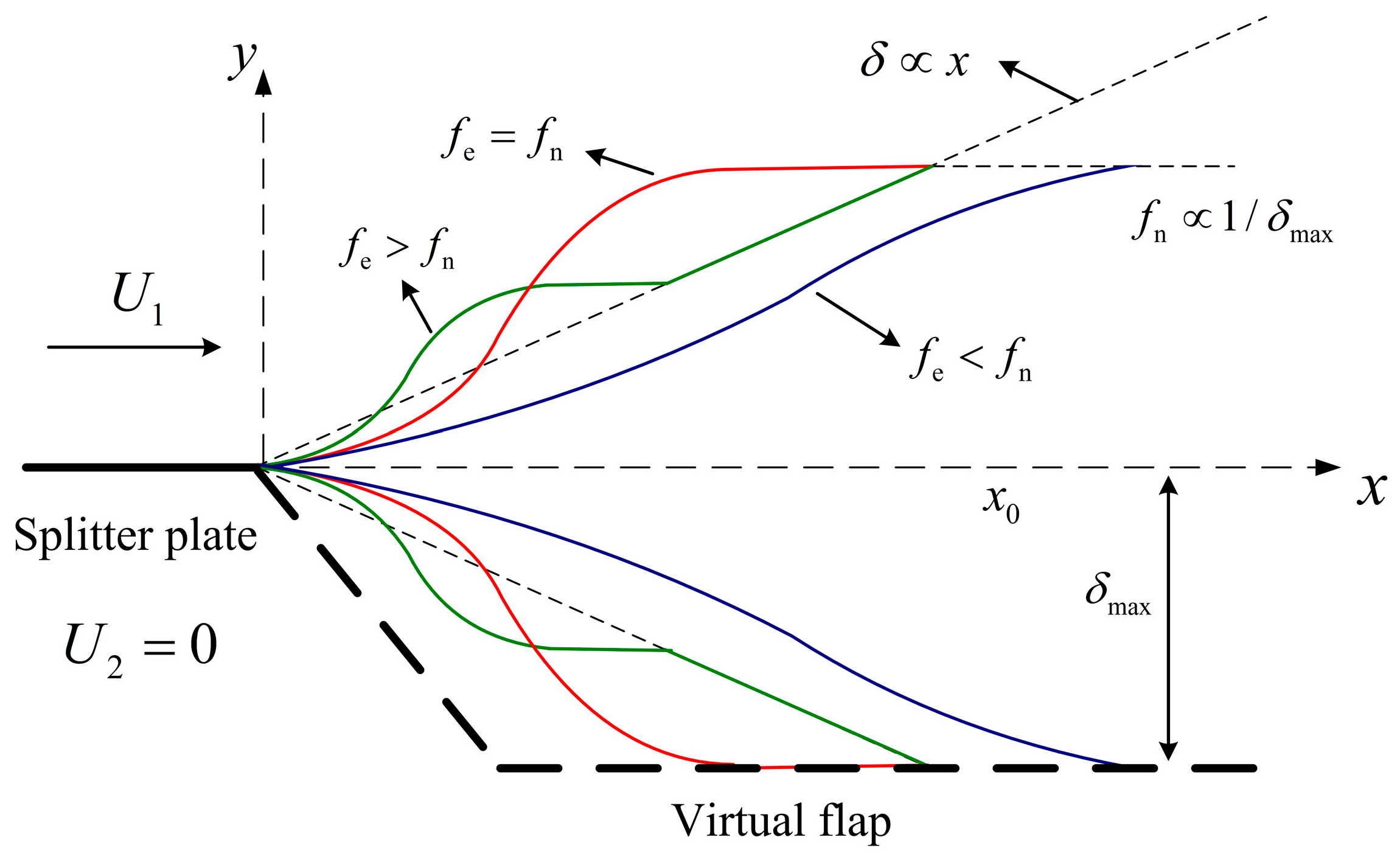
Figure 11.
Non-dimensional growth rate of perturbation () versus non-dimensional distance (, which is to the initial position of instability).
Figure 11.
Non-dimensional growth rate of perturbation () versus non-dimensional distance (, which is to the initial position of instability).


Table 1.
Typical unsteady flow control methods.
| Unsteady Flow Control Methods | Brief Description |
|---|---|
| Acoustic excitation | Acoustic excitation is produced by a sound source and is used to excite the boundary layer to control its transition or separation |
| Synthetic jet | Synthetic jet uses the wall vibration of a cavity to form periodic suction and blowing. Its mass flow input is zero, while momentum output is not zero. |
| Pulsed jet | Pulsed jet uses high-pressure air sources and periodically opens and closes valves to form periodic jet disturbance. |
| Wall oscillation | Wall oscillation is set a movable wall, which can vibrate periodically at the appropriate position, so as to reduce the flow resistance or separation. |
| Traveling wave wall | Traveling wave wall control originated from bionics. Proper Travelling Wave can capture a series of stable vortices and separate the mainstream from the wall (serving as “Fluid Roller Bearings”), resulting in the reduction of flow resistance or separation. |
| Plasma actuator | Plasma actuator uses the plasma motion under electromagnetic force or the temperature and pressure changes caused by gas discharge to control the flow field. |
© 2019 by the authors. Licensee MDPI, Basel, Switzerland. This article is an open access article distributed under the terms and conditions of the Creative Commons Attribution (CC BY) license (http://creativecommons.org/licenses/by/4.0/).
Share and Cite
MDPI and ACS Style
Lu, W.; Huang, G.; Wang, J.; Yang, Y. Interpretation of Four Unique Phenomena and the Mechanism in Unsteady Flow Separation Controls. Energies 2019, 12, 587. https://doi.org/10.3390/en12040587
AMA Style
Lu W, Huang G, Wang J, Yang Y. Interpretation of Four Unique Phenomena and the Mechanism in Unsteady Flow Separation Controls. Energies. 2019; 12(4):587. https://doi.org/10.3390/en12040587
Chicago/Turabian StyleLu, Weiyu, Guoping Huang, Jinchun Wang, and Yuxuan Yang. 2019. "Interpretation of Four Unique Phenomena and the Mechanism in Unsteady Flow Separation Controls" Energies 12, no. 4: 587. https://doi.org/10.3390/en12040587
Note that from the first issue of 2016, this journal uses article numbers instead of page numbers. See further details here.