Modelling Influential Factors of Consumption in Buildings Connected to District Heating Systems

Energy Institute Hrvoje Požar, 10000 Zagreb, Croatia
Energies 2019, 12(4), 586; https://doi.org/10.3390/en12040586
Submission received: 15 January 2019
/
Revised: 9 February 2019
/
Accepted: 11 February 2019
/
Published: 13 February 2019
(This article belongs to the Special Issue 4th International Conference on Smart Energy Systems and 4th Generation District Heating)
Abstract
:Assessing the influential factors on measured (or allocated) heat consumption in district heating systems is often limited by the available data. Within a project of modelling consumption in district heating systems in Croatia for the Ministry of Environmental Protection and Environment, an access to a complete billing database of the largest Croatian district heating company was granted. The company supplies approximately 126,400 final consumers (both households and businesses) over 375 km of distribution network. The billing database has 40 vectors in a few million single inputs. In addition to these data, a questionnaire is distributed to the final consumers in several buildings labelled as “model buildings”, gathering behavioural and demographic data of final consumers (such as occupancy, mode of space usage, heat comfort level, age of occupants, etc.). The two sets of data are then merged, and a correlation analysis is performed. Furthermore, a two-step regression analysis is performed based on variables from billing database in the first step, with added behavioural and demographic variables obtained from the questionnaires in the second step. The models from two steps are compared, tested and interpreted. Results of the most influential factors on heat consumption in district heating systems are given and the influence of the behavioural/demographic variables on the prediction accuracy of heating consumption is interpreted.
1. Introduction
The building sector in the European Union consumes around 40% of total final energy consumption, of which about 80% is spent on heating and domestic hot water preparation (the remainder consists of cooling with 0.6% and electric energy with 19.40%) [1]. The first major incentive to increase energy efficiency and reduce energy consumption was made after the signing of the Kyoto Protocol [2], which encouraged various approaches and methodologies for increasing energy efficiency in buildings, particularly in residential buildings [3]. In contemporary research, a number of models have been developed to evaluate the effects of applying energy efficiency measures and forecasting consumption in the building sector, based on methods such as traditional regression methods [4], neural networks [5] and various simulation methods [6]. The International Energy Agency (IEA) recognises two basic approaches to energy consumption and energy savings assessment, namely, “top-down” and “bottom-up” approaches, for which the IAE has provided detailed guidance for calculations [7]. The “bottom-up” approach can be based on the physical properties of buildings, statistical models or may be a hybrid. In the EU, the “bottom-up” model is predominantly used when determining incentive legislative frameworks to achieve energy efficiency, but its main disadvantage is the fact that such models are inadequate in describing non-technical influential parameters and introduce a greater number of model assumptions related to behavioural aspects of energy consumption such as demographic factors, age of final consumers, daily disposition of space usage, consumer willingness to pay, etc. [8].
Recently, an increasing research focus has been put on the aforementioned numerous non-technical factors affecting energy consumption. Thus, Yang and et al. consider the behaviour of the space user and the level of thermal comfort [9]. Furthermore, Nguyen et al. analyse intelligent systems for monitoring the use and control of energy consumption in buildings [10]. With the increase of available data on non-technical parameters of consumption and the development of data collection technologies, the analysis of these data has the potential to support a better understanding and modelling of energy consumption due to a series of non-technical factors. When analysing big data, statistical methods are used, such as Olofsson et al., using basic coordinate analysis and regression method of partial least squares to determine the main influencing factors for energy consumption in district heating systems, electricity consumption, potable water consumption and heat losses [11]. Furthermore, machine learning algorithms, predominantly a support vector machine, are shown to be suitable for assessing energy consumption in buildings [12,13].
By changing the energy policy within the EU, district heating systems have been identified as one of the main instruments for achieving the goals of increasing energy efficiency and increasing the share of renewable energy sources in the energy mix [14,15]—indicating the need for precise methods of estimating consumption and saving energy in these systems. In February 2016, the European Commission issued the first strategy for optimization of heating and cooling in Member States, which illustrates the overall efficiency of these systems in the future [16]. At the end of 2012, the European Parliament and the Council of the European Union adopted Directive 2012/27/EU on energy efficiency, the primary objective of which is to achieve energy savings of 20% by 2020 and to open new energy efficiency improvements after this period. Also, in Article 9 of the abovementioned Directive, introduction of individual distribution of heat energy consumption in district heating systems, has been identified as the basic prerequisite for achieving energy savings by changing user behaviour [17]. Compared to the energy consumption in the general building stock, additional influencing factors in the district heating systems refer to the existence or absence of individual consumption measurement, the existence of DHW preparation or lack thereof, the possibility of replacing the primary energy source, the amount and management of heat losses in the distribution system, and valorisation of passive heat gains in multi-storey buildings [18]. The estimate of the effect of individual measurements of heat energy consumption by using a heat cost allocator (HCA) was experimentally performed in the seventeen-year period by measuring consumption in two identical housing units (equally entering the same building) so that heat cost allocators are incorporated in one unit, while in the other they are not. The annual savings achieved in the unit with built-in heat cost allocators are about 27% [19]. Such estimated savings cannot be uniquely attributed to the impact of installing heat cost allocators, because energy consumption is influenced by numerous factors. Previously, a great deal of research has been conducted in order to describe and understand the energy consumption in the residential sector. Most of the accessed categories of objectives are identified in these three categories: (i) energy, (ii) occupants’ behaviour and (iii) guidelines (in energy policies or simulation and design) [20]. In this paper an emphasis is placed on occupant behaviour related data, and the questionnaire is made with the focus on this area. The questions about relevant parameters in the questionnaire and interviews conducted in this paper where based on previous research carried out in Denmark and the Netherlands [21,22]. As Croatia is located in southern Europe, the relevant parameters defined for the northern countries of Denmark and the Netherlands where double-checked with the parameters defined for Greece [23].
The goal of this paper is to make an initial classification of influential factors on heat consumption in the buildings connected to district heating systems with cross-referencing parameters from both billing data and questionnaires on behavioural and demographic characteristic.
This paper is organised as follows: Section 2 describes materials and methods used in this paper, while Section 3 presents the results of the research performed. Finally, Section 4 reports the discussion.
Research Background and Motivation
The Energy Efficiency Directive (2012/27/EU) was transposed into the Croatian legislation in the Heat Market Act (Official Gazette 80/13, 14/14 and 95/15) and the Energy Efficiency Act (Official Gazette no. 127/14). According to the mentioned acts, it was necessary to install electronic heat cost allocators (abbreviated HCA) or heat energy meters and thermostatic radiator valves in all residential/business premises connected to the district heating systems by the end of 2016.
Starting from 2010 in its new, energy legislation, based on EU principles and requirements regarding energy sector organisation and functioning, as well as promoting energy efficiency, the Republic of Croatia has opted for a model in which each residential area, regardless of whether they are multiapartment buildings or a family homes, has its own access to all network services and its own measurement of the service performed. For efficient energy use it is essential that the owner of the living space can decide on how energy is used so that his energy consumption can be measured and paid as much as it is spent. Prior to the introduction of individual allocation or of heat consumption measurement, actual consumption was measured on the building level and then equally allocated based on the floor area with no “energy-based” measurements on the apartments level.
However, most of the apartments that were constructed prior to 1995 and are connected the district heating systems (DHS) in buildings have a vertical distribution system, meaning that one vertical pipe goes through each room on each floor so the apartments do not have a single input/output point. In these apartments it was not economically viable to provide direct heat consumption measurement without a technically and financially demanding reconstruction of the heating installation within the building. For such cases the installation of HCA was allowed as a more economically feasible option.
HCAs are devices attached to individual radiators in buildings that allocate the total heat output of the individual radiator within apartment. For efficient energy use it is essential that the final consumer has an opportunity to measure the actual energy used in a specific unit and billed based on the actual consumption. Numerous studies and analyses have confirmed that by installing HCAs, annual heat savings at the heat station level (i.e., the entire building) can be expected at the level from 15% to 30% [19]. The achieved savings, i.e. reduced heat consumption, are further distributed to each individual consumer by a certain allocation methodology. However, the installation of HCAs in Croatia caused great dissatisfaction for a number of final consumers. A total of 70 complaints of final customer submitted by four energy entities performing the activity of supplying heat to households and industrial subjects, i.e., the activity of the buyer and a consumer protection association, were analysed. The analysed complaints can be classified into the following three groups with regard to the subject of the complaint: complaints against the excessive bill for the delivered heat energy and preparation of hot water, requirements for information and dissatisfaction with the overall heat energy consumption calculation system.
The final motivation of this work presented in this paper is to develop a model that would be used for the purposes of assessing the effects introducing individual metering has had on the heat consumption in district heating, on household, building, network and national levels.
2. Materials and Methods
2.1. Analysed Dataset
In the course of analysing the effects of implementation of individual metering in district heating systems in Croatia, with the aim of resolving the issues described in the previous text, access to the anonymised billing data was granted in 2016. Furthermore, during 2018 questionnaires were distributed to 154 apartments with a short set of straightforward questions with the aim of obtaining information on presumed influential factors on heat consumption of which no information can be find in the billing data. In close cooperation with the tenants’ official representative the questionnaires were distributed to the tenants and a total of 51 tenants participated in the interviews, making a share of 33.55%. Furthermore, the tenants’ representative provided anonymised metering data for all of the 154 apartments. The questionnaires were not anonymised, and all of the participants were required to give their consent for the participation in this scientific research based on the EU General Data Protection Regulation [20]. The consents obtained were presented to the local district heating company with the request for access to the relevant billing data for the 51 apartments participating in the interviews (“participating apartments” in the following text). All of the relevant technical and metering data for the building were obtained from the participating apartments’ billing data. Pairing the billing data with the anonymised metering data obtained from the tenants’ representative provides a data set for the analysis presented in this paper. This paper is based on the available data from two sets, as follows:
- (1)
- The first data set consists of actual billing data for the final consumers.
- (2)
- The second data set is based on the questionnaires distributed to the apartment owners (tenants).
The analysed building is located in Zagreb, Croatia, and it consists of three sub-divisions, where each subdivision has its own heating substation. The type of all substations is indirect. The ground plan outlook of the building is given in Figure 1.
The building’s sub-divisions for the purposes of this paper will be named as follows:
- (1)
- Subdivision A (SD_A)
- (2)
- Subdivision B (SD_B)
- (3)
- Subdivision C (SD_C)
The relevant characteristics of each subdivision are given in Table 1.
Each of the sub-divisions is connected to a separate heating substation and has an individual heat meter. This paper encompasses analyses made for 2016 and 2017.
2.1.1. Billing Data
The billing data was accessed based on the consents from 51 participating apartments. The request for the access to data was submitted to the local district heating company and the data was provided. The provided data is an integral part of a monthly bill submitted to each apartment owner. The outlook of the bill is shown in Figure 2.
The required data was a subset of all of the available billing data at the district heating company, and was defined as:
- (1)
- Customer code
- (2)
- Code of the heat meter
- (3)
- Building area
- (4)
- Building area of the customers with HCAs
- (5)
- Heaters’ thermal power (installed thermal capacity) of the customers with HCAs
- (6)
- Heaters’ thermal power (installed thermal capacity) of the customers without HCAs
- (7)
- Total metered heat
- (8)
- Total number of impulses from all of HCAs in the building
- (9)
- Number of impulses from the specific participating apartment
- (10)
- Floor area of participating apartment
The above listed data was obtained on a monthly basis, in accordance to the billing frequency. Allocation of heat energy consumption for an individual consumer is made in accordance with the applicable rules, as laid down by the Regulation on the Method of Distribution and Calculation of Costs for the Delivered Heat Energy (Official Gazette, br. 99/14, 27/15, 124/15) [24,25].
The allocation formula used to allocate heat consumption in the buildings with HCA installed is:
where: ESUC—heat energy allocated to an individual unit [kWh]; EG—total delivered heat energy in the calculation period for space heating (without sanitary hot water preparation) measured on a common building heat energy meter without the heat energy allocated to units without HCAs installed [kWh]; PGSUC—the surface of all independent use units that had the heat energy consumption in the calculating period [m²]; PSSUC—the surface of all independent use units on a common heat energy meter [m²]; UR—percentage of the delivered heat energy on a common meter of heat energy calculated according to the proportion of number of impulses read in the independent use unit in the total number of impulses read in all independent use units (%); BIR—number of readings impulses of all devices for local distribution of delivered heat energy in independent use unit [-]; BIRU—total number of readings impulses of all devices for local distribution of delivered heat energy at a common heat energy meter [-]; UPOV—percentage of the delivered heat energy on a common meter of heat energy calculated according to the proportion of the surface of an independent use unit on the surface of all independent use unit (%); PSUC—the surface of an independent use unit provable to the actual surface, not diminished or otherwise changed [m²]; ESUC—part of the delivered heat energy for an independent use unit [kWh]; IESUC—the amount of energy cost for the independent use unit [HRK]; CTE—specific price of the heat energy [HRK/kWh].
Billing data was supplemented with available HCA readings for all of the building’s apartments, as well as the defined building related characteristics, such as the heated area of each apartment. By merging these two data sources a full dataset of quantitative predictors was established and used in further analysis.
2.1.2. Questionnaire and Interviews
The second data source this paper is based on was gathered via questionnaires and personal interviews in the analysed multiapartment building. The questionnaire’s content, the list of relevant questions and structure are given in Table 2.
This paper aims to provide an overview of the influential factors affecting the consumption in district heating systems for both technical (or physical) and non-technical (or behavioural) factors. The technical factors are considered to be the parameters that could be measured or stated from the physical characteristics of the buildings or read from the available metering devices, and generally it could be said that these factors are available from the billing data and can be clearly stated and addressed. On the other hand, behavioural data cannot be clearly stated interviews with the final consumers need to be carried out. Based on previous research and experience, the survey’s questions were formulated to include these relevant sections (see Table 2):
- Information on the age structure and the number of the tenants: this section contained questions about the age structure of the tenants in years prior to and after the installation of HCAs. This information is considered to be important with the presumption that certain age groups (specifically, children under the age of 7 and retirees) spend scientifically more time in their apartments then school children, students and people in work. Additionally, the presumption is that the desired heat comfort level for children under the age of 7 years is higher than that for other groups. The answer to this question is asked for the years 2010–2017, while 2015 was the year HCA were installed in this building. The categories of age groups have been defined as:
- ○
- Ages 0–6 years
- ○
- Ages 7–18 years
- ○
- Ages 19–65 years
- ○
- Ages 65 and more
- The information of the floor is asked for the purposes of assessing the influence on the consumption of the location of the specific apartment within the building.
- Information on the daily occupancy time: this section is grouped within three groups as shown in Table 2.
- Information on the existence of the efficient windows.
- Information on the type of the windows: in this section participants needed to quality their window types in predefined categories. Predefined categories are chosen based on the knowledge of the most usual windows type in Croatia, as shown in Table 2.
- Preferred heat comfort level: assessed in three categories.
- Number of unheated rooms: historically in this geographic area there is a custom not to heat the rooms person/family is not using during the daytime.
- Average daily ventilation rate: the last question is related to the influence of the ventilation rate of the apartment on the consumption and it is presumed to be a behavioural parameter of a significant influence.
2.2. Statistical Analysis
The statistical analysis in this paper was performed using R programming language [26], with the aim of evaluating the influential factors on heat consumption in district heating systems, based on the available data for Zagreb, Croatia. For the purposes of this paper libraries tidyverse, readxl, tibble, dplyr, ggplot2, summarytools, packagemetrics, sjPlot and nortest were used. The regression coefficients where finally calculated with a “lm” function.
2.2.1. Frequency Density of Qualitative Variable
Frequency density of a certain parameter is the occurrence of this particular parameter in a total class size, and it is defined as:
where: Pi is the relative frequency; ni is the absolute frequency.
2.2.2. Frequency Density of Qualitative Variable
Descriptive statistics of quantitative data was done with R’s “summary” function giving these relevant data for the predictors dataset:
- (1)
- Mean: For arithmetic mean a measure of central tendency.
- (2)
- Standard Deviation: Measure the amount of variation using the square root of the variance and gives an information how close are all of occurrences clustered around the mean of a particular dataset.
- (3)
- Minimum Value: Gives a minimum value in a dataset.
- (4)
- Q1 Value: Gives a middle value between the minimum value and median in a dataset.
- (5)
- Median: The measure the central tendency giving the middle value in dataset.
- (6)
- Q3 Value: Gives a middle value between the median and the maximum value in a dataset.
- (7)
- Maximum Value: Gives a maximum value in a dataset.
- (8)
- Median Absolute Deviation: A scale estimate based on the median absolute deviation.
- (9)
- Interquartile range (IQR): A measure of the spread between the 1st and 3rd quartile.
- (10)
- Coefficient of variation or relative standard deviation (CV): Represents a ration between standard deviation and a mean, or a spread relative to its expected value.
- (11)
- Skewness: Measure of the symmetry of the distribution. Positive skewness indicates a tail on the right side of the graph, while negative skewness indicates a tail on a left side of the graph. A value of skewness of zero indicates a symmetric distribution or an asymmetric distribution when “fat and short tail” is balancing the “long and thin tail”.
- (12)
- Standard Error of Skewness: Standard deviation or a sampling distribution of skewness.
- (13)
- Kurtosis: Describes the shape of the distribution or the outlook of tails in the distribution, describing the tails based on the kurtosis as either heavy or light. Positive kurtosis is called leptokurtic and indicates a distribution with heavier tails than a normal distribution. Negative kurtosis is called platykurtic and indicates a distribution with lighter tails than a normal distribution.
2.2.3. Frequency Density of Qualitative Variable
Normality of the analysed data is tested graphically, by testing and comparing histogram graphs with the normal probability curve and by the producing normal probability plot. Furthermore, Shapiro-Wilk of univariate normality is performed for the dependant variable, specific heat consumption per heated floor area (kWh/m2). The testing is done using R, with the function “shapiro.test”.
In order to determine if the data is following the normal distribution a p-value is compared to a significance level. A significance level for this analysis is considered to be 0.05. If the p-value for the analysed dataset is less or equal, than the significance level it can be concluded that the data does not follow the normal distribution. Hence, if the p-value is larger than the significance level, we can conclude that we cannot conclude that the analysed dataset doesn’t follow the normal distribution, but we still cannot conclude that it does before performing additional tests. The additional test to be performed is the visualisation test.
2.2.4. Frequency Density of Qualitative Variable
The datum was analysed using multiple the linear regression model, defining each of the vectors from the data frame consisting of both Billing Data and Questionnaire Data either as predictors or as a dependant variable of interest. For this model the dependant variable of interest is the specific heat consumption in an individual apartment as a function of the remaining variables we define as independent variables or independent predictors.
The multiple linear regression is represented as:
where: Xi is the i-th predictor; b0 is the intercept; bi is a regression coefficient, defines the association between the variable and the response. In essence, the regression coefficients Bi give a measure of an average influence of a predictor Xi on F(X), when all other predictors are fixed. The multiple regression model was based on a set of independent variables from both Billing Data and Questionnaire Data while holding specific heat consumption per a specific dwelling as a dependent variable. The relevant variables selection was based on previous research described in this paper, as well as on findings based on the interviews performed. The relevant independent variables for this regression models are:
F(X) = b0 + b1X1 + b2X2 + … + biXi,
Quantitative predictors:
- (1)
- Monthly number of impulses from HCAs in an individual apartment (from Billing Data, denoted—ID_Imp)
- (2)
- Monthly total number of all HCA impulses in a building (from Billing Data, denoted—B_Imp)
- (3)
- Total metered heat on a main building heat meter (from Billing Data, denoted—B_E_MWh)
- (4)
- Heated floor area of an individual apartment (from Billing Data, denoted—m2)
- (5)
- Monthly absolute allocated heat to an individual apartment (from Billing Data, denoted—Ap_MWh)
- (6)
- Monthly specific heat consumption in kWh per m2 (from Billing Data, denoted—Ap_kWh_m2)
- (7)
- Specific monthly ratio of total impulses from HCAs of an individual apartment relative to heated floor area (from Billing Data, denoted—Imp_m2)
- (8)
- Total number of dwellers in an individual apartment (from Billing Data, denoted—Dwellers)
Qualitative predictors:
- (1)
- Floor (from both Billing Data and Questionnaire Data, denoted Floor)
- (2)
- Average daily occupancy of an individual apartment (from Questionnaire Data, denoted AverageDailyOccupancy)
- (3)
- Data on efficiency of apartment’s windows (from Questionnaire Data, denoted EfficientWindows)
- (4)
- Data on type of apartment’s windows (from Questionnaire Data, denoted EffWindowType)
- (5)
- Data on the desired heat comfort level (from Questionnaire Data, denoted ThermalComfort)
- (6)
- Data on number of unheated rooms (from Questionnaire Data, denoted UnheatedRooms)
- (7)
- Data on estimated ventilation rate (from Questionnaire Data, denoted Ventilation)
- (8)
- Total number of dwellers in an individual apartment (from Billing Data, denoted—Dwellers)
It can be seen that the total number of dwellers parameter has been double categorised as both a quantitative and qualitative predictor. This is needed for the reason of fitting this variable into the multiple linear regression where we want it to be included as a qualitative predictor. On the other hand, this predictor can be a quantitative predictor at the same time, e.g., for the purposes of expressing the specific consumption per dweller. As can be seen from the list above, the data from the dataset Billing Data are quantitative predictors, while the data from the dataset Questionnaire data are qualitative. Whilst regression of quantitative predictors is straightforward, when introducing qualitative predictors (or factors) in models an introduction of a helper indicator or dummy variable is needed.
3. Results
3.1. Normality of Data
3.1.1. Shapiro-Wilk Normality Test
The result of Shapiro-Wilk Test for the analysed dataset is given in Table 3.
The significance level is p ≥ 0.05. Based on the results we cannot conclude that the data do not follow the normal distribution and visualization of the fit is conducted as an additional test.
3.1.2. Visualising the Fit
In this section the normality of the dependant variable on an annual basis will be reported. For this purpose, the specific monthly heat consumptions from the billing dataset were summarised separately for 2016 and 2017. The boxplots with the associated distribution curve are presented in Figure 3.
As it can be seen in Figure 3, following the distribution line over the box plots and the two presented normality plots, the data for an approximation of a straight line, so we can conclude that the normal distribution is a good fit for the analysed dependant variable based on the visualisation test.
3.2. Frequencies of Qualitative Parameters from Questionnaires
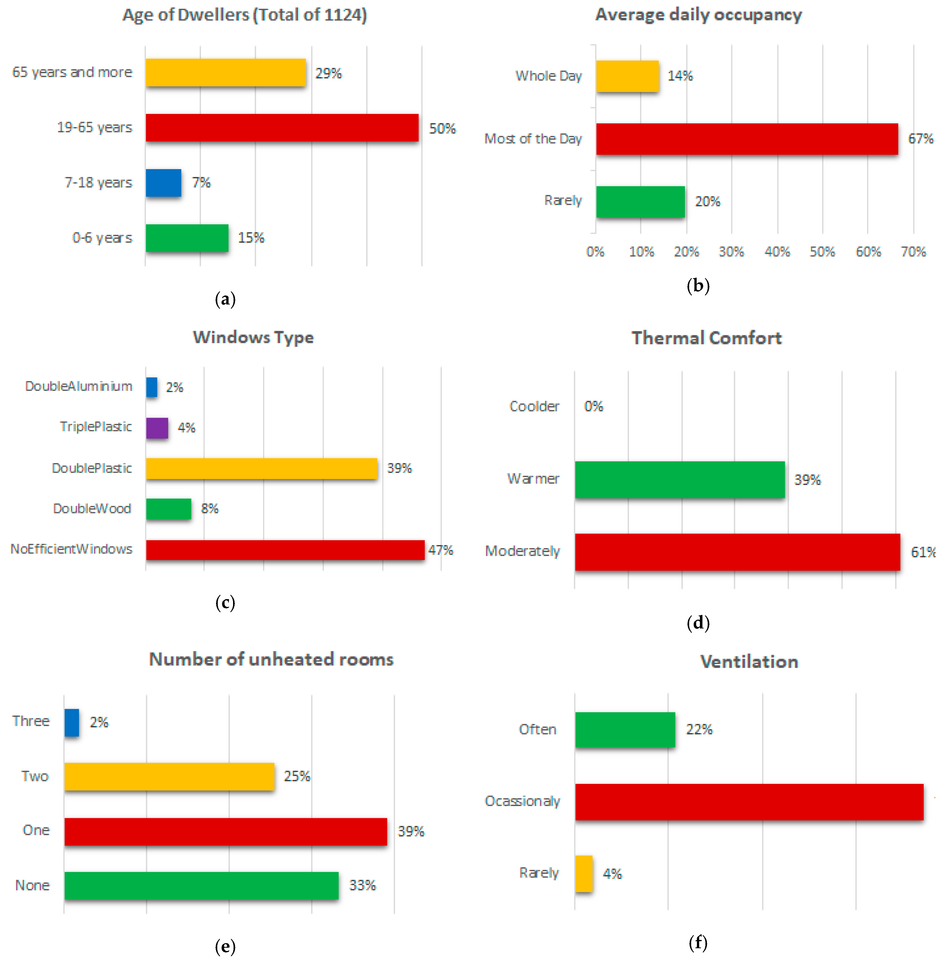
In this section the results of the frequency density analysis of the relevant data gathered through the questionnaires is presented (see Figure 4).
As can be seen from Figure 4, most of the dwellers from the participating apartments are between the ages of 19 to 65 (working force category). As well, it can be concluded that most of the participants stay at home most of the day, prefer moderately warm thermal comfort level in the apartments that have no efficient windows, heat most of the rooms and open the windows in the heating season just occasionally. The influence of ventilation is presumed to be of importance and will be further accessed when interpreting multiple regression model.
3.3. Descriptive Statistics
3.3.1. Quantitative Predictors
Table 4 provides summary statistics for the relevant quantitative predictors from the analysed dataset.
The dependant variable is denoted as “Ap_kWh_m2” and represents the parameter of specific heat consumption for each of the 150 analysed apartments in the building. This parameter is the dependable variable for the regression model and will be described in more detail.
The range of the dependable variable “Ap_kWh_m2”, in kWh/m2, is from 0.13 kWh/m2 (Minimum) to 50.16 kWh/m2. The mean. as an arithmetic average of the data is 11.88 kWh/m2 monthly. The median as the midpoint of the dataset is close to the mean –10.27 kWh/m2. The first quartile value is 3.68 kWh/m2. while the third quartile value is 17.75 kWh/m2.
The standard deviation of the data is 9.54 kWh/m2. If we consider the standard deviation to be a measure of spread of the data from the mean (mean being 11.88 kWh/m2), we can see that these two values are on the similar level. Pairing what has been stated with the coefficient variance of 0.80. both these values can further indicate a normality of this particular parameter.
The skewness of data is positive. with the value of 0.80. indicating that the skewness is positive. the distribution is slightly to the right. but still close to the value of zero indicating that the data is symmetrical (assuming the values of asymmetry from −2 to +2).
The kurtosis value of 0.34 indicates that the distribution of the dependable variable dataset has somewhat heavier tails and a sharper peak.
3.3.2. Correlations and Relationships of Quantitative Variables
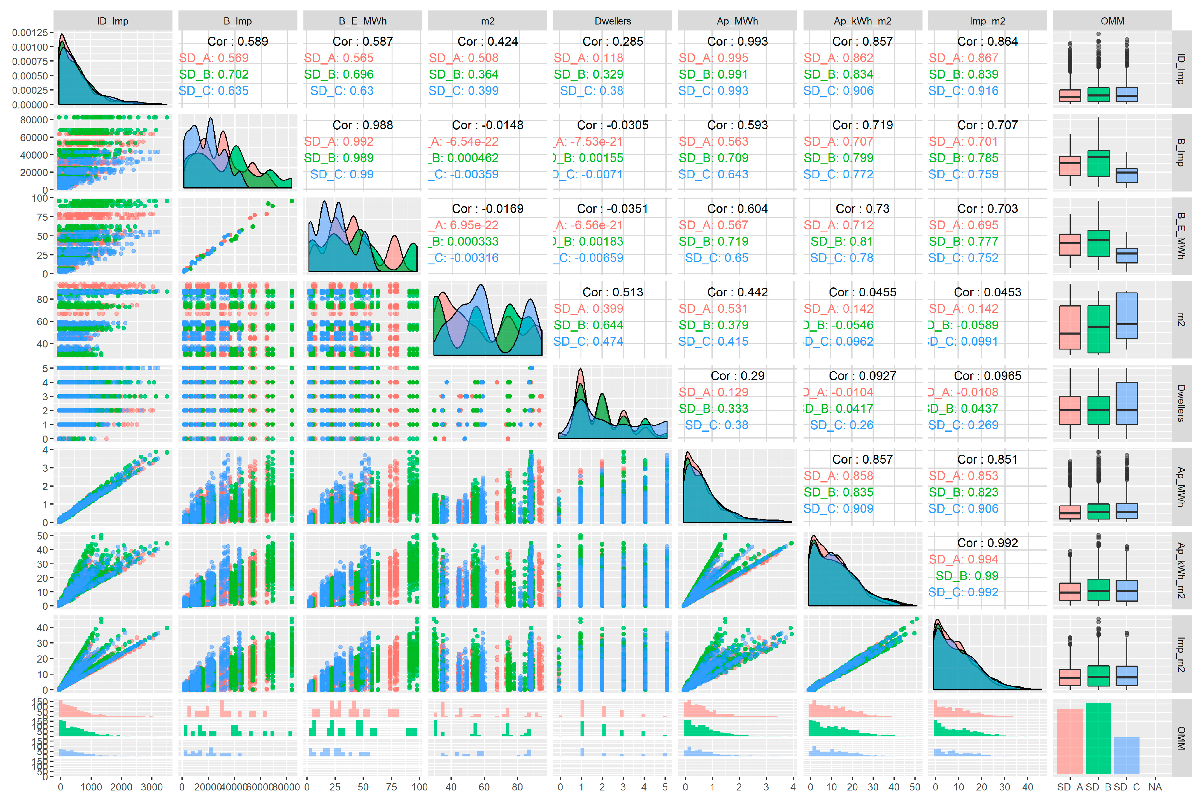
Furthermore, the correlation and relationships within all of the quantitative variables is given in Figure 5 using a matrix plot. Additional variable used compared to the dataset of quantitative variables to produce this plot is a quantitative (or categorical) variable “OMM”. This variable indicates the building sub-division and has the values SD_A. SD_B and SD_C (see Table 1.).
Looking at the upper right triangle pane of the matrix plot in Figure 5 correlation coefficients can be interpreted for each of the pairs of the relevant quantitative variables. The correlation coefficients comprise the values between −1 and 1, and are interpreted as:
- −1 indicates a strong negative correlation (can be interpreted as variable A increases. variable A decreases)
- 0 indicates no correlation between the pair of variables. and.
- 1 indicates strong positive correlation (can be interpreted as variable A increases. variable B increases as well).
The lower left triangle pane on the matrix plot presents the scatter plots of the pairs of the relevant variables. The diagonal plots differentiate the trends of the pairs of relevant variables taking into consideration the quantitative (or categorical) variable “OMM”.
3.3.3. Visualising the Sample Distributions
Additionally, it is considered that the visualisation of the dependable variable for each of the analysed apartments is important. As it was said in the introduction and motivation for the research presented in this paper, the strongest motivation to address the influential factors on heat consumption and possible heat consumption savings was found in the unexpected dissatisfaction of the final consumers in the district heating systems after the HCAs had been installed. For this reason. addressing and analysing each of the individual apartments is important, especially to identify the individual apartments with the occurrence of outliers in the categories of relevant values (in this paper this is the value of the specific heat consumption per apartment).
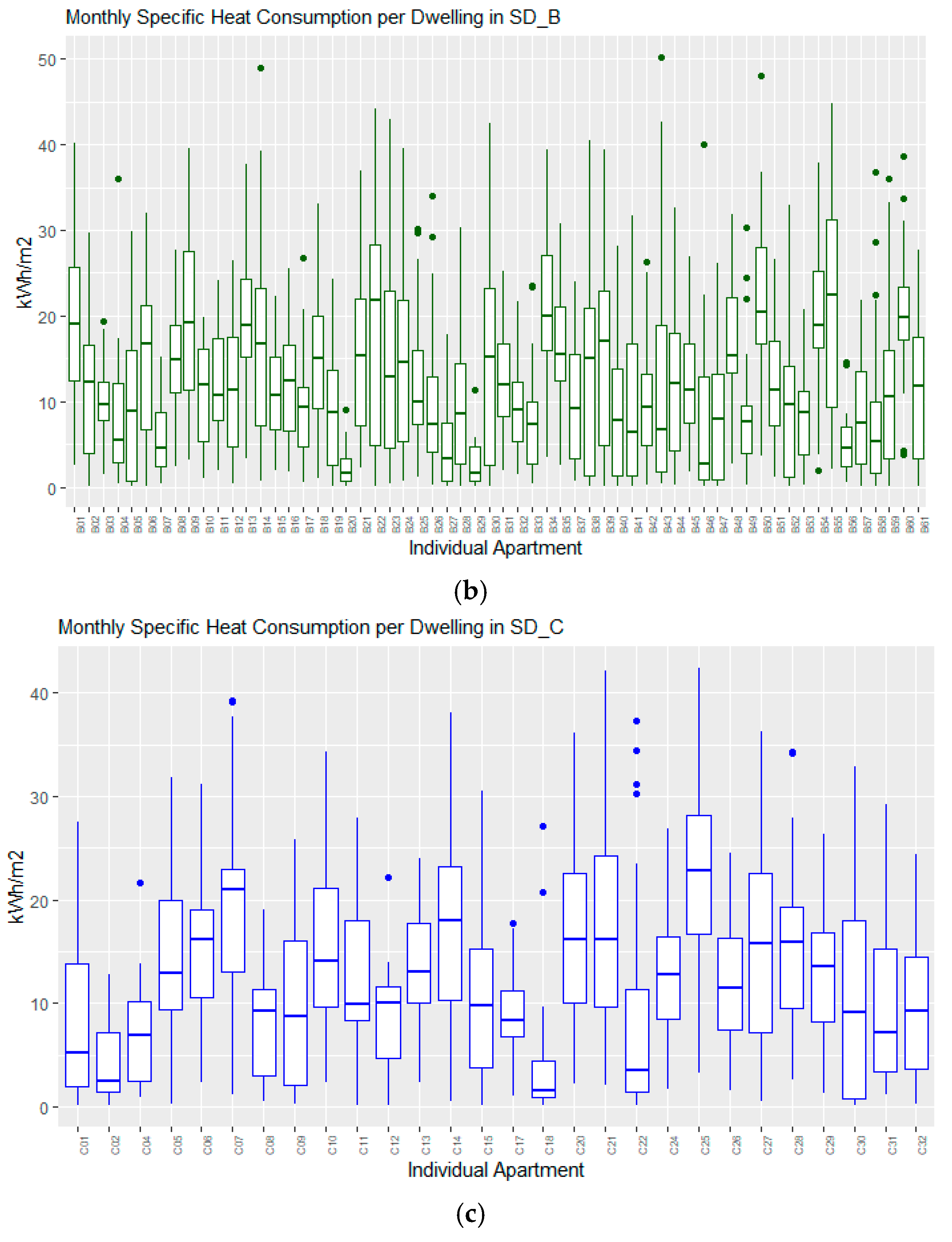
In the first step, the visualisation was made for each of the building’s subdivision (see Figure 6), as there is considered to be a physical difference between each of the subdivisions and each of them is connected to a different heating substation and has separate heat meters.
The largest sub-division, Sub-division B, has the largest range of the relevant dependable variable. This can be explained by the fact that the statistical sample is the largest for this subdivision and the fact that all of the apartments in this subdivision have implemented HCAs. Looking at Figure 5, it can be said that the expected range of the specific heat for this building is within the range of 5 to 20 kWh/m2 per month during the heating season. The values can be lower, and if so, this can be interpreted that there is a high possibility that the apartment was vacant in the considered month.
The picture shows the spread for the maximum values, as well as the outliers recorder. It can be seen that the maximum monthly value was recorded in Subdivision B. As this record has a singular occurrence, this gives an indication that the reason for this high consumption can probably be attributed to a malfunction of the HCAs in a given month. In Figure 7 boxplot representations for individual apartments have been presented for the whole building and for each subdivision separately.
3.3.4. Qualitative Predictors
Prior to calculating the regression coefficients for the qualitative predictors, a visualisation of the correlation between dependable variable and the qualitative predictors values obtained from the questionnaires was made and is given in Figure 8. The findings of the analysis of the influence of each of the qualitative predictors from questionnaires are:
- (1)
- Total number of dwellers in an individual apartment. The largest spread of values is found, as expected, in the apartment with the largest number of dwellers.
- (2)
- Floor. The largest specific consumption was recorded for the basement apartments, as expected.
- (3)
- Average daily occupancy of an individual apartment. No distinguished influence of the daily occupancy mode on the heat consumption can be interpreted. It can be concluded that the apartments in which dwellers stay most of the day can be expected to have the largest spread of values for the specific consumption.
- (4)
- Efficiency of apartment’s windows. As expected, apartments without efficient windows have larger heat consumption.
- (5)
- Type of apartment’s windows. Type of windows are presented.
- (6)
- Desired heat comfort level. As expected, apartments with requirements for warmer ambient temperature have larger consumption. None of the apartments that have participated in survey have stated they preferred colder thermal comfort level.
- (7)
- Number of unheated rooms. No distinguished influence of the daily occupancy on the specific consumption can be interpreted.
- (8)
- Ventilation rate. As expected, larger specific heat consumption is recorded in apartments with larger frequency of ventilation of space by opening the windows, while the mean for all three groups (often, occasionally and rarely) is at a similar level.
To further evaluate the influence of each qualitative predictors on heat consumption, all of the analysed predictors will be analysed and included in the multiple linear regression model.
3.4. Multiple Linear Regression Analysis
Results of the regression are given relative to the dependable variable specific heat consumption per individual apartment. “Ap_kWh_m2” are reported in Table 5. The first column of the table annotates the independent variables. The second column contains estimated values of the regression coefficients (“Estimate”). The third column gives standardised values of the regression coefficients. The fourth column represents standard deviation values and the last column gives the p-values.
It can be noticed that the quantitative variables have been listed as multiple independent variables at the number that equals one less (n−1) of the number of possible answers to the questions related to the qualitative variable in the questionnaire. The reason for this is the way regression model treats and codes qualitative variables. In this particular case, the regression model makes so-called dummy variables. the number of which is always one fewer then the levels of the variable.
Looking at Table 5, the findings can be formulated as:
- The most influential factor among quantitative variables are the number of impulses in the apartment. allocated and measured heat for both the apartment and the building, and the ratio between allocated impulses and the area (the most significant factor).
- Among the quantitative variables the largest influence is recorded from the particular window type, following the daily occupancy rate and frequency of ventilation.
- The adjuster R2 for the analysed model is 0.998, meaning that 99.8% of analysed data can be explained by the variables obtained in Table 5.
- If we were to express the function using Equation (5), the “Estimates” in the Table 5 would be equivalent to the regression coefficients (bi), while the predictors would have a Xi value.
4. Discussion
Although most studies dealing with assessing energy savings after the introduction of individual metering (either by individual heat meters or heat cost allocators) in buildings connected to district heating systems have reported significant savings [19], no comprehensive assessment of the savings at the level of an individual apartment has been made. At the same time, the experience in implementing the EU Energy Efficiency Directive in the part of individual metering in Croatia, has shown that a large number of final consumers did not achieve the presumed savings, but have even significantly increased their cost for heat. This fact was a motivation for conducting research into a comprehensive assessment on influential factors on consumption in buildings connected to district heating systems.
In this paper influential factors on the energy consumption in buildings connected to DH systems are defined as technical (mostly quantitative variables) and non-technical (mostly qualitative variables), whereby the non-technical forms of consumption include social and behavioural aspects, such as demographic factors, the daily schedule of the use of space and others. This represents the originality of this paper as most of the previous analyses and models, like the research done by Juodis [27], predominantly delved into technical factors only.
When analysing the data comprising both technical and non-technical data, where technical data was available from the billing data and non-technical data was obtained by virtue of questionnaires, at this level of research it can be concluded that significant influential factors on heat consumption are the ratio between the metered values (for HCA these are impulses) and the heated area, window type, daily occupancy rate and frequency of ventilation.
Further research is planned based on the findings of this paper. A model for a typical building will be developed based on the qualitative data and merged with a large available database on heat consumption, as described in the Introduction.
Based on the model presented in this paper, the next step will be to implement machine learning algorithms and statistical methods together with comparative analysis and identification of the most appropriate algorithm to analyse the separate effect of energy efficiency measures installing individual measurements in buildings heated from heating systems to reduce energy consumption.
The final goal of this research is to develop a model that would be used for the purposes of assessment of the effects of introducing the individual metering on the heat consumption in district heating, on households, buildings, networks and at a national level.
Supplementary Materials
Supplementary File 1Funding
This research received no external funding.
Conflicts of Interest
The authors declare no conflict of interest.
Abbreviations
| IEA | International Energy Agency |
| EU | European Union |
| DHW | Domestic Hot Water |
| HCA | Heat Cost Allocators |
| DHS | District Heating Systems |
| SD-A | sub-division A of the analysed building |
| SD-B | sub-division B of the analysed building |
| SD-C | sub-division C of the analysed building |
| HRK | Croatian Kuna, currency |
| IQR | Interquartile Range |
| CV | Coefficient of Variation |
References
- Fraunhofer and Alia. Mapping and Analyses of the Current and Future (2020–2030) Heating/Cooling Fuel Deployment (Fossil/Renewables); ENER/C2/2014-641; Fraunhofer and Alia: Berlin, Germany, 2015. [Google Scholar]
- International Energy Agency. Energy Efficiency Market Report 2015; International Energy Agency: Paris, France, 2015. [Google Scholar]
- de Boeck, L.; Verbeke, S.; Audenaert, A.; de Mesmaeker, L. Improving the energy performance of residential buildings: A literature review. Renew. Sustain. Energy Rev. 2015, 52, 960–975. [Google Scholar] [CrossRef]
- Catalina, T.; Virgone, J.; Blanco, E. Development and validation of regression models to predict monthly heating demand for residential buildings. Energy Build. 2008, 40, 1825–1832. [Google Scholar] [CrossRef]
- Haghighat, L.M.F. Multiobjective optimization of building design using TRNSYS simulations genetic algorithm and Artificial Neural Network. Build. Environ. 2010, 45, 739–746. [Google Scholar]
- Al-Ajmi, F.F.; Hanby, V.I. Simulation of energy consumption for Kuwaiti domestic buildings. Energy Build. 2008, 40, 1101–1109. [Google Scholar] [CrossRef]
- International Energy Agency. Mapping the Energy Future: Energy Modelling and Climate Change Policy; Energy and Environment Policy Analysis Series; International Energy Agency: Paris, France, 1998. [Google Scholar]
- Kavgic, M.; Mavrogianni, A.; Mumovic, D.; Summerfield, A.; Stevanovic, Z.; Djurovic-Petrovic, M. A review of bottom-up building stock models for energy consumption in the residential sector. Build. Environ. 2010, 45, 1683–1697. [Google Scholar] [CrossRef]
- Yang, L.; Yan, H.; Lam, J.C. Thermal comfort and building energy consumption implications—A review. Appl. Energy 2014, 115, 164–173. [Google Scholar] [CrossRef]
- Nguyen, T.A.; Aiello, M. Energy intelligent buildings based on user activity: A survey. Energy Build. 2013, 56, 244–257. [Google Scholar] [CrossRef] [Green Version]
- Olofsson, T.; Andersson, S.; Sjogren, J.U. Building energy parameter investigations based on multivariate analysis. Energy Build. 2009, 41, 71–80. [Google Scholar] [CrossRef]
- Jain, R.K.; Smith, K.M.; Culligan, P.J.; Taylor, J.E. Forecasting energy consumption of multi-family residential buildings using support vector regression: Investigating the impact of temporal and spatial monitoring granularity on performance accuracy. Appl. Energy 2014, 123, 168–178. [Google Scholar] [CrossRef]
- Smola, A.J.; Vishwanathan, S.V.N.; Le, Q.V. Bundle Methods for Machine Learning. In Advances in Neural Information Processing Systems 20; Platt, J.C., Koller, D., Singer, Y., Roweis, S., Eds.; MIT Press: Cambridge, MA, USA, 2008. [Google Scholar]
- Lund, H.; Möller, B.; Mathiesen, B.V.; Dyrelund, A. The role of district heating in future renewable energy systems. Energy 2010, 35, 1381–1390. [Google Scholar] [CrossRef]
- Thellufsen, J.Z.; Lund, H. Energy saving synergies in national energy systems. Energy Convers. Manag. 2015, 103, 259–265. [Google Scholar] [CrossRef]
- Commision to the European Parlament the Council. The European Economic and Social Committee and the Committee of the Regions. An EU Strategy on Heating and Cooling; Commision to the European Parlament the Council: Brussels, Belgium, 2016. [Google Scholar]
- European Commission. Directive 2012/27/Eu of the European Parliament and of the Council of 25 October 2012 on Energy Efficiency. Amending Directives 2009/125/EC and 2010/30/EU and repealing Directives 2004/8/EC and 2006/32/EC. 2012. Available online: https://www.energypoverty.eu/publication/directive-201227eu-european-parliament-and-council-25-october-2012-energy-efficiency (accessed on 7 January 2019).
- Siggelsten, S. Reallocation of heating costs due to heat transfer between adjacent apartments. Energy Build. 2014, 75, 256–263. [Google Scholar] [CrossRef]
- Cholewa, T.; Siuta-Olcha, A. Long term experimental evaluation of the influence of heat cost allocators on energy consumption in a multifamily building. Energy Build. 2015, 104, 122–130. [Google Scholar] [CrossRef]
- Carpino, C.; Mora, D.; de Simone, M. On the use of questionnaire in residential buildings. A review of collected data methodologies and objectives. Energy Build. 2019, 186, 297–318. [Google Scholar] [CrossRef]
- Andersen, R.V.; Toftu, J.; Andersen, K.K.; Olesen, B.W. Survey of occupant behaviour and control of indoor environment in Danish dwellings. Energy Build. 2009, 41, 11–16. [Google Scholar] [CrossRef]
- Santin, O.G. Behavioural Patterns and User Profiles related to energy consumption for heating. Energy Build. 2011, 43, 2662–2672. [Google Scholar] [CrossRef]
- Sardianou, E. Estimating space heating determinants: An analysis of Greek households. Energy Build. 2008, 40, 1084–1093. [Google Scholar] [CrossRef]
- Regulation (EU) 2016/679 of the European Parliament and of the Council of 27 April 2016 on the Protection of Natural Persons with Regard to the Processing of Personal Data and on the Free Movement of Such Data. And Repealing Directive 95/46/EC (General Data Protection Regulation). Available online: https://www.lewik.org/term/13554/regulation-eu-2016-679-of-the-european-parliament-and-of-the-council-of-27-april-2016-on-the-protection-of-natural-persons-with-regard-to-the-processing-of-personal-data-and-on-the-free-movement-of-such-data-and-repealing-directive-95-46-ec-general-data-protection-regulation-gdpr/ (accessed on 7 January 2019).
- Regulation on the Method of Distribution and Calculation of Costs for the Delivered Heat Energy (Official Gazzette. br. 99/14. 27/15. 124/15). Available online: https://narodne-novine.nn.hr/clanci/sluzbeni/2014_08_99_1956.html (accessed on 7 January 2019).
- R Core Team. R: A Language and Environment for Statistical Computing; R. Foundation for Statistical Computing: Vienna, Austria, 2018; Available online: https://www.R-project.org/ (accessed on 7 January 2019).
- Juodis, E.; Jaraminiene, E.; Dudkiewicz, E. Inherent variability of heat consumption in residential buildings. Energy Build. 2009, 41, 1188–1194. [Google Scholar] [CrossRef]
Figure 1.
Ground floor plan of the analysed building: (a) Satellite image from Google Maps; (b) A sketch of the ground plan with the annotations of the each subdivision.
Figure 1.
Ground floor plan of the analysed building: (a) Satellite image from Google Maps; (b) A sketch of the ground plan with the annotations of the each subdivision.

Figure 2.
Outlook of the heat bill provided to the apartments in the analysed building and issued by the local district heating company.
Figure 2.
Outlook of the heat bill provided to the apartments in the analysed building and issued by the local district heating company.

Figure 3.
Box plot and normality plot visualisation of the specific annual heat consumption for 150 apartments with installed HCA: (a) Box plot for 2016; (b) Box plot for 2017; (c) Normality plot for 2016; (d) Normality plot for 2017.
Figure 3.
Box plot and normality plot visualisation of the specific annual heat consumption for 150 apartments with installed HCA: (a) Box plot for 2016; (b) Box plot for 2017; (c) Normality plot for 2016; (d) Normality plot for 2017.

Figure 4.
Results of the frequency analysis of the relevant questions from questionnaires, based on the 51 participating apartment owners: (a) Structure of the age of dwellers; (b) Daily occupancy of the analysed apartments; (c) Windows type; (d) Desired thermal comfort level; (e) Number of the unheated rooms; (f) Ventilation rate of the participating apartments.

Figure 5.
Matrix plot of relevant quantitative variables.

Figure 6.
Boxplots of the monthly specific heat consumption in each subdivision.

Figure 7.
Visualisation of box plot diagrams for each analysed individual apartment: (a) Apartments in Subdivision A. (b) Apartments in Subdivision B. (c) Apartments in Subdivision C.
Figure 7.
Visualisation of box plot diagrams for each analysed individual apartment: (a) Apartments in Subdivision A. (b) Apartments in Subdivision B. (c) Apartments in Subdivision C.


Figure 8.
Visualisation of box and whisker plots for each analysed qualitative predictor, representing quartiles, the median, minimum and maximum of data and outliers: (a) Specific consumption relative to the number of dwellers; (b) Specific consumption relative to the floor on which apartment is located. (c) Specific consumption relative to daily occupancy. (d) Specific consumption relative to the existence of energy efficient windows. (e) Specific consumption relative to the type of windows. (f) Specific consumption relative to the desired level of thermal comfort. (g) Specific consumption relative to the number of unheated rooms. (h) Specific consumption relative to the ventilation rate.


Table 1.
Relevant building characteristics per each sub-division.
| Characteristics | SD_A | SD_B | SD_C |
|---|---|---|---|
| Total floor area | 3383.18 | 3500.04 | 1880.53 |
| Total number of apartments | 61 | 61 | 32 |
| Total number of apartments with HCA | 58 | 61 | 31 |
| Floor area of apartments with HCA | 3246.79 | 3500.04 | 1793.56 m2 |
| Floor area of apartments without HCA | 136.39 | 0 | 86.97 m2 |
| Thermal capacity of apartments with HCA | 410.731 | 394.260 | 227.389 kW |
| Thermal capacity of apartments without HCA | 17.254 | 0 | 11.026 kW |
| Total number of tenants | 111 | 128 | 70 |
| Number of floors | 6 | 6 | 5 |
Table 2.
Questionnaire structure and content.
|
Table 3.
The result of the p-value Shapiro-Wilk Normality Test.
| Dataset for Year | p |
|---|---|
| 2016 | 0.2151 |
| 2017 | 0.0975 |
Table 4.
Summary statistic of quantitative data in the analysed dataset.
| Value | ID_Imp | B_Imp | B_E_MWh | m2 | Dwellers | Ap_MWh | Ap_kWh_m2 | Imp_m2 |
|---|---|---|---|---|---|---|---|---|
| Mean | 548.74 | 28,901.33 | 38.27 | 57.66 | 2.09 | 0.69 | 11.88 | 9.39 |
| .Stand. Deviation | 545.79 | 19,716.36 | 24.69 | 20.4 | 1.25 | 0.65 | 9.54 | 8.04 |
| Min | 0 | 2140 | 3.05 | 29.72 | 0 | 0 | 0.13 | 0 |
| Q1 | 133 | 12,720 | 21.71 | 35.3 | 1 | 0.19 | 3.68 | 2.5 |
| Median | 406 | 24,663 | 32.94 | 55.37 | 2 | 0.54 | 10.27 | 7.77 |
| Q3 | 781 | 41037 | 51 | 73.98 | 3 | 0.97 | 17.75 | 14.24 |
| Max | 3444 | 82,382 | 95.91 | 92.99 | 5 | 3.89 | 50.16 | 45.26 |
| MAD | 453.68 | 18,925.39 | 20.87 | 27.89 | 1.48 | 0.56 | 10.26 | 8.55 |
| IQR | 648 | 28,317 | 29.29 | 38.68 | 2 | 0.78 | 14.07 | 11.74 |
| CV | 0.99 | 0.68 | 0.65 | 0.35 | 0.6 | 0.94 | 0.8 | 0.86 |
| Skewness | 1.6 | 0.71 | 0.66 | 0.16 | 0.75 | 1.55 | 0.87 | 0.91 |
| SE. Skewness | 0.05 | 0.05 | 0.05 | 0.05 | 0.05 | 0.05 | 0.05 | 0.05 |
| Kurtosis | 3.04 | −0.14 | −0.26 | −1.35 | −0.36 | 2.83 | 0.34 | 0.44 |
| Number. Valid | 2465 | 2465 | 2465 | 2465 | 2465 | 2465 | 2465 | 2465 |
| Percentage. Valid | 99.96 | 99.96 | 99.96 | 99.96 | 99.96 | 99.96 | 99.96 | 99.96 |
Table 5.
Summary statistic of quantitative data in the analysed dataset.
| Predictors | Estimate | Standardised (βi) | Std. Error | p | Sign. Code 1 |
|---|---|---|---|---|---|
| (Intercept) | 0.833 | 0.000 | 0.167 | <0.001 | *** |
| No of impulses for an apartment | −0.014 | −0.819 | <0.001 | <0.001 | *** |
| No of impulses for a building | <0.001 | −0.207 | <0.001 | <0.001 | *** |
| Total heat for a building in MWh | 0.086 | 0.218 | 0.006 | <0.001 | *** |
| Heated floor area of an apartment | −0.008 | −0.018 | 0.001 | <0.001 | *** |
| Number of tenants | 0.006 | 0.001 | 0.016 | 0.722 | - |
| Allocated MWh per apartment | 11.730 | 0.831 | 0.270 | <0.001 | *** |
| Ratio between number of impulses and area | 1.166 | 0.985 | 0.005 | <0.001 | *** |
| Daily occupancy—rarely | −0.124 | −0.005 | 0.039 | 0.001 | ** |
| Daily occupancy—whole day | −0.049 | −0.002 | 0.048 | 0.305 | - |
| Efficient Windows—partly | −0.093 | −0.002 | 0.140 | 0.508 | - |
| Efficient Windows—yes | −0.179 | −0.005 | 0.122 | 0.141 | - |
| Windows Type—Plastic Double Glass | −0.178 | −0.009 | 0.099 | 0.073 | . |
| Windows Type—Wooden Double Glass | −0.064 | −0.002 | 0.113 | 0.575 | - |
| Windows Type—No Efficient Windows | −0.074 | −0.004 | 0.101 | 0.464 | - |
| Windows Type—Plastic | 0.026 | 0.001 | 0.119 | 0.825 | - |
| Thermal Comfort—Warmer | 0.030 | 0.002 | 0.034 | 0.379 | - |
| Unheated Rooms—One | 0.001 | <0.001 | 0.040 | 0.983 | - |
| Unheated Rooms—Three | −0.256 | −0.004 | 0.119 | 0.032 | * |
| Unheated Rooms—Two | −0.115 | −0.005 | 0.048 | 0.018 | * |
| Ventilation—Often | −0.077 | −0.003 | 0.037 | 0.036 | * |
| Ventilation—Rarely | 0.133 | 0.003 | 0.078 | 0.090 | . |
| Observations | 836 | - | - | - | - |
| R2 /adjusted R2 | 0.998/0.998 | - | - | - | |
1 Significance code: Signif. codes: 0 ‘***’ 0.001 ‘**’ 0.01 ‘*’ 0.05 ‘.’ 0.1 ‘ ’ 1.
© 2019 by the author. Licensee MDPI, Basel, Switzerland. This article is an open access article distributed under the terms and conditions of the Creative Commons Attribution (CC BY) license (http://creativecommons.org/licenses/by/4.0/).
Share and Cite
MDPI and ACS Style
Maljkovic, D. Modelling Influential Factors of Consumption in Buildings Connected to District Heating Systems. Energies 2019, 12, 586. https://doi.org/10.3390/en12040586
AMA Style
Maljkovic D. Modelling Influential Factors of Consumption in Buildings Connected to District Heating Systems. Energies. 2019; 12(4):586. https://doi.org/10.3390/en12040586
Chicago/Turabian StyleMaljkovic, Danica. 2019. "Modelling Influential Factors of Consumption in Buildings Connected to District Heating Systems" Energies 12, no. 4: 586. https://doi.org/10.3390/en12040586
Note that from the first issue of 2016, this journal uses article numbers instead of page numbers. See further details here.