EV Idle Time Estimation on Charging Infrastructure, Comparing Supervised Machine Learning Regressions

Abstract

The adoption of electric vehicles (EV) has to be complemented with the right charging infrastructure roll-out. This infrastructure is already in place in many cities throughout the main markets of China, EU and USA. Public policies are both taken at regional and/or at a city level targeting both EV adoption, but also charging infrastructure management. A growing trend is the increasing idle time over the years (time an EV is connected without charging), which directly impacts on the sizing of the infrastructure, hence its cost or availability. Such a phenomenon can be regarded as an opportunity but may very well undermine the same initiatives being taken to promote adoption; in any case it must be measured, studied, and managed. The time an EV takes to charge depends on its initial/final state of charge (SOC) and the power being supplied to it. The problem however is to estimate the time the EV remains parked after charging (idle time), as it depends on many factors which simple statistical analysis cannot tackle. In this study we apply supervised machine learning to a dataset from the Netherlands and analyze three regression algorithms, Random Forest, Gradient Boosting and XGBoost, identifying the most accurate one and main influencing parameters. The model can provide useful information for EV users, policy maker and network owners to better manage the network, targeting specific variables. The best performing model is XGBoost with an R² score of 60.32% and mean absolute error of 1.11. The parameters influencing the model the most are: The time of day in which the charging sessions start and the total energy supplied with 22.35%, 15.57% contribution respectively. Partial dependencies of variables and model performances are presented and implications on public policies discussed.

1. Introduction

The energy transition of our time does not aim for a change of energy sources alone. It comes with a smarter and sustainable drive, bringing together energy systems and communication technologies domains, creating the gold of our era: Information. Digitalization promises to help improve the safety, productivity, efficiency and sustainability of many sectors and energy systems are no exception. The most revolutionary changes could come in road transportation. Its partial electrification, connectivity and automation technologies could fundamentally transform how citizens plan their lives, how goods are moved and how services are provided. At the beginning of 2018 there were close to half a million publicly accessible electric vehicles (EV) chargers worldwide, and more than three million electric vehicles [1] generating millions of observations and valuable datasets.

City and regional traffic authorities make use of data to manage and promote public policies of shared spaces. Across all transport modes, digital technologies and collection of data are helping to improve energy use, reduce maintenance costs and improve customer service. In road transport, real-time information on location and routing can help optimize vehicle and fleet operations. Connectivity also enables a wide range of other operations, from checking the status of an EV battery state of charge, track free charging spaces or inform about the charging status, all available in a simple smartphone app [2]. To this regard, digitalization is playing a major role in supporting alternative fuel vehicle adoption, especially EVs and the roll-out of its associated charging infrastructure. An effective roll-out of public charging infrastructures, has been identified as crucial to promote EV adoption in theEuropean Union (EU) directive 2014/94/EU on the deployment of alternative fuels infrastructure [3]. EV infrastructure has hence gained the attention of the scientific community and policy makers. Charging infrastructure data have been used extensively, covering a wide range of topics, however it can be set into two main categories: Infrastructure analysis and user behavior studies.

The correct sizing of the infrastructure is an important topic for investors and policy makers, to offer consumers the correct range of availability within given areas, promoting the adoption of EVs and the correct use of space. Digitalization and the use of Big Data, have been playing a major role in managing and planning systems in the last years and will play a major role in years to come. The European Joint Research Centre (JRC) has developed a methodology [4] providing a broad overview of the applications of a data processing platform, designed to harness the potential of big data in the field of road transport policies in Europe. The platform created, uses data from navigation systems focusing on mobility and driving patterns. The methodology and results presented show howbig data could be used for policy assessment and better governance.

The use of real data has made possible the development of performance indicators studies for the charging infrastructure, which, despite scarce, capture important and key concepts to be taken in consideration [5,6,7,8]. Targeting the improvement of charging station deployment, a study [5] using real-world data, provides a new approach for municipalities, by treating the infrastructure as a complex network of charging stations and defining vulnerability in respect to the availability of its surrounding charging stations, within relevant walking distance. Based on two vulnerability measures: (i) Service failure vulnerability (ii) inconvenience vulnerability, the authors suggest that the cities under study, should deploy future chargers based on the spatial distribution of charging stations, with high vulnerability scores. They hence recommend implementing additional charging stations on the outskirts of the city, in order to reduce service failure, and in the city center in order to reduce inconveniences for EV users in case of charging station failure. In an exercise to understand results and performance of a public charging network, authors in Reference [6] focus on main stakeholders in the infrastructure deployment and EV adoption and gather their main concerns and objectives. They categorize these inputs as 10 key results and 14 performance indicators. With the goal of designing a slow-charging infrastructure with maximum covered demand, a study [9] develops an optimization problem defining levels of service. The study clearly distinguishes between daytime and night-time charging needs, which may be estimated by residential and employment information of a certain region under study.

The size of the infrastructure is estimated by local authorities and using different regression methods, the authors have been able to estimate charging needs on specific areas in the city of Lisbon.

In a study analyzing a dataset capturing 2014 and 2015 years [7] in the Netherlands, the authors developed eight quantitative performance metrics, providing a common methodology to compare and analyze different charging infrastructures. The authors used the following indicators: Energy demand from EVs, energy use intensity, charger’s intensity distribution, the use time ratios, energy use ratios, the nearest neighbor distance between chargers and availability, the total service ratio, and the carbon intensity of the chargers themselves corresponding to the life cycle analysis of the materials involved. Authors reject the approach of using km, population size or number of cars to evaluate the charging infrastructure size and fit. Authors report major contributions by proposing several indicators using energy units, for example: 4040.23 MJ_{year/connector}, instead of 10 vehicles per connector. During the study the authors find the idle time (vehicle connected without charging time) to be on average 61.4% of the total connected time (Connected time = charging time + idle time). Authors carry on discussing that idle time reduces the availability of the chargers, leaving EV users with an unknown waiting time option, or having to approach the second-best charging option which can be several kilometers away. They conclude that this fact may undermine the perception of EV users or wrongly hint the infrastructure to be undersized, unless the idle time is managed and monitored.

With the understanding and study of charging infrastructures, architectures and online platforms [10,11], have been created to inform different stakeholders on the analytics and status of the system. These platforms contain mainly information, such as charging profiles, times of use, number of charging points and locations. Another study [8] presents a methodology to process Big Data gathered from charging sessions. This architecture contains a web interface and allows users to get information on the performance of the charging infrastructure such as location, use status or total time of use per charger.

Apart from infrastructure studies, there is also the need to understand user’s behaviors and preferences. Understanding consumer’s behavior means identifying and understanding patterns through data science. Data mining and exploratory data analysis studies have been developed to explore numbers beyond their simple acquisition. A study [12] on the factors influencing connection times of EV to charging stations, was developed applying a multinomial logistic regression technique. Major findings demonstrate that time-of-day-related factors and the charging station rated power influence the duration of the connection to the charging station the most. More precisely, the connection duration to level 2 chargers (up to 11 kW) is very much associated with parking preferences. The authors justify this by the lower charging capacity of these stations, motivating EV users to leave their vehicle parked at a charging station for a longer time while being at work or home.The dataset under study refer to the years 2014 to 2016 and indicate that a substantial percentage of the charging sessions last more than 24 hours. Authors call for the attention of policy makers defending that simply providing charging infrastructure coverage will not automatically meet charging needs in every zone. This is due to the fact that the types of dwellings help determining the connection duration and also the timing of the charging session. Zones with mostly one type of dwelling are expected to experience peak demand, while mixed areas with different sizes and building congifurations and types could assist different users with fewer chargers, making use of the demand variation over time. Still on charging behavior characterization, an article [13] presents different charging patterns to try and benchmark behaviors. The study focuses on five city areas with an extensive public charging infrastructure to establish whether and how charging behavior differs between cities. The total connection time is mentioned as a potential problem to EV satisfaction, as many chargers seem to be occupied even after the charging process is completed. The authors state that Taxis, often with larger battery packs than the average EV, are responsible for overall higher use of energy (kWh) and also more kWh per charge session. Although car sharing only makes up a small portion of the users, these vehicles tend to be responsible for having the highest numbers of charge sessions.

A study [14] on the parking times and influences public policies may have on user’s behavior on charging sessions, was developed for the city of the Hague. The study describes the implementation of daytime limitation of parking spots using signs next to charging stations. These parking spots would be exclusively available between 10:00 and 19:00 for electric vehicles and accessible for other vehicles beyond these determined hours. Major findings from the study show that implemented daytime charging 10–19 h, can restrict EV owners in using the charging station at times when they need it. A shift of demand was observed from late afternoon to morning periods. The study also considered an extension of the dedicated EV charging time from 10 to 22, and did not observe a significant change. The study is however a useful exercise demonstrating how connection sessions can be limited through public policies and its impacts studied.

It is in fact a crucial point, if cities are going to manage connection time of sessions, idle time has to be known and measured. From the literature it can be understood that, regardless of the acceptable amount of idle time, which may vary from location to location, from the point of view of the user, its excessive use introduces a negative impact on the infrastructure, impacting the availability, sizing and cost. From a smart charging perspective, idle time is seen as an opportunity to shift the charging period. In this sense from a Distribution System Operator (DSO) point of view, idle time is not experienced as a negative impact. Even though the charging time can be accurately estimated, to the best of our knowledge, the idle time estimation has been overlooked. This study hence, applies three well known supervised machine learning algorithms in regression: Random Forest, Gradient Boosting, and XGBoost. We use an original 1.8 million observation (charging sessions) dataset, acquired in the Netherlands and focus on the years of 2014 up to June 2018. A comparison between the model’s accuracy metrics will be presented, the variables identified and how their dynamics impact the target variable.

2. Regression Algorithms

Among supervised machine learning algorithms there are several options to estimate output of continuous nature. The algorithms chosen in this study are very similar to each other, but contain small variations which may make the difference in improving accuracy when analyzing the dataset under study. Random Forest (RF) was chosen for being easy to use and to understand. It has also shown robustness in data training with large quantities of events and is intrinsically suitable for multi-class problems. Gradient Boosting and XGBoost follow similar approaches as RF in using trees, but differ especially in its Hyperparameters, performing sometimes better than RF and are hence worth exploring.

2.1. Random Forrest Regressor

Random Forest is an ensemble learning method developed by Breiman [15] and is commonly used for both classification and regression problems. The main idea behind the algorithm is to grow a set of regression trees, hence the name forest. First, the algorithm starts with a number of bootstrap samples from the original dataor predictor space. Each of these samples will generate a regression tree with an adjusting operation, in which afterwards a number of the predictors are randomly sampled. The algorithm goes on choosing the best split from the group of the sampled variables, instead of considering them all as a whole. The square root of the total number of variables is assumed by the algorithm as the default number of the predictors’ value. Thus, it is recommended the use of a high number of trees. RF does not tend to over fit when more trees are added [15] and provides a limited error when generalizations are made.

The outcome of the model is estimated using the mean value of the individual predictions provided by each decision tree. An advantage of using RF is that it does not need difficult pre-treatment of data which is often very time consuming and runs relatively fast when compared to other algorithms. The main shortcoming of RF is that using large number of trees may slow down the algorithm making it unsuitable for real time prediction for example.

This method is also much easier to tune than other regression algorithms, such as Gradient Boosting (GB). There are typically two hyperparameters in RF: the number of features to be selected at each node and the number of trees.

Real World applications are various, such as to determine a stock’s behavior in the future, or in the healthcare domain where it is used to identify the correct combination of components in medicine and to analyze a patient’s medical history to identify diseases. Also, in E-commerce RF is used to determine whether a customer will actually like a product or not.

2.2. Gradient Boosting Regressor

Similarly to RF, also GB combines the outputs from individual trees, thus called an ensemble learning method. The original idea of the method was introduced by Breiman [16], when it realized that boosting could be interpreted as an optimization of a cost function. Regression gradient boosting algorithms were later introduced by different authors [17,18,19,20], exploring the notion of boosting algorithms as iterative functional gradient descent algorithms. The idea behind is optimizing a cost function by iteratively choosing a function (weak hypothesis) that points in the negative gradient direction.

GB and RF contrast in the manner in which the trees are assembled, such as the order and the way the results are combined. Gradient boosting has revealed [21] great performance on real life datasets, especially in ranking exercises due to two major characteristics.

It starts by developing an optimization in function of space, which facilitates the use of custom loss functions. Then it focuses on a step by step basis, which gives a nice strategy to deal with unbalanced datasets, by strengthening the impact of the positive class.

A shortcoming of GB is the tendency to overfitting if the data is noisy. For this reason cross validation or other suitable techniques are advised, which may be more time consuming. Furthermore, training generally takes longer due to the fact that trees are built in sequence. GB hyperparameters are also more difficult to optimize than RF ones. There are usually three important hyperparameters to consider when optimizing: Number of trees, depth of trees and learning rate. Application of GBM is anomaly detection in supervised learning settings where data is often highly unbalanced, such as DNA sequences, credit card transactions or cyber security.

2.3. XGBRegressor

XGBoost [22] is a more recent development in machine learning but follows the principle of gradient boosting, containing some differences in modeling details. XGBoost uses a more normalized model description to control over-fitting, which usually provides a better overall performance.

The motivation for the XGBoost concept comes from the technical will to improve the performance of computational power for boosted tree algorithms. This method is hence one of the fastest to implement tree ensemble approaches, while taking into account the potential loss of different splits made in creating a new branch in the tree. This of course may be regarded as an inefficient process, but the algorithm mitigates this by observing the distribution of features across all data points in a leaf, and uses this information to decrease the search space of potential feature splits.

Among all the hyperparameters there are typically five which are known to influence the model the most: Number of subtrees to be trained (n_estimators), maximum tree depth each tree can grow (max_depth), learning rate, reg_alpha and reg_lambda are regularization terms influencing the weight at the leaves and the scattering. Many real-world problems have missing data that for itself contains valuable information about the target. All use cases used in other regressors could be applied to XGBoost.

2.4. Hyperparameters

A hyperparameter in the machine learning domain is a consideration of values defined before training a given model. On the other hand the parameter values themselves are derived via the actual training. The type of hyperparameters and their quantity differ from algorithms to algorithm. There are even some simple algorithms which require none, such as the ordinary least squares regression for example. Having defined a set of hyperparameters, when a specific model is trained, it will learn the parameters from the data. Hyperparameters are used to define the depth of the model, the ability to learn or some preferences on the construction of the trees and so cannot be learned from the data. As mentioned in the algorithms brief descriptions, some examples of hyperparameters are: Number of leaves or depth of a tree, learning rate (in various models), number of hidden layers in a deep neural network, number of clusters in a k-means clustering approach just to mention a few.

The n_estimators hyperparameter, which is the number of trees the algorithm builds before taking the maximum voting or taking averages of predictions. In general, a higher number of trees increases the performance and makes the predictions more stable, but it also slows down the computation. Another important hyperparameter is max_features, which is the maximum number of features a Random Forest for example is allowed to try in an individual tree.

The n_estimators hyperparameter, is the number of trees the algorithm builds. Typically, a higher number of trees increases the performance and makes the predictions more stable, but it also reduces the processing speed. Another important hyperparameter is max_features, which refers to the maximum number of features a certain model is allowed to try in an individual tree. The min_sample_leaf hyperparameter determines the minimum number of samples that are required to split a node and create a new leaf. In this study all these main hyperparameters will be optimized using built in libraries in the tools used for applying the algorithms.

3. Methodology

3.1. The Dataset

The original raw data was obtained through ElaadNL [23], a Dutch smart charging knowledge center promoted by a grid operators consortium, and comprises the registers of charging stations and user interactions. This historical data of transactions, was gathered from January 2012 until June 2018 of 1747 public charging stations which are operated by EVnetNL, with 1 or 2 connectors (2911 connectors in total), installed throughout the entire country of the Netherlands. The charging stations are all three-phase connected, with a maximum rated power of 22 kW. In the year 2015, the dataset represented 16% of all the charging stations installed in the Netherlands [11]. The raw dataset has approximately 1,823,449 charging events (transactions) and the parameters are registered with the corresponding timestamp using Universal Time Coordinated (UTC) units. From the transaction identifier (user’s card), it has been possible to estimate 82,301 EV drivers who have used the charging stations during the observation period. Such users’ cards (RFID) are hashed and replaced by a string of 64 characters. By doing so, the data can be used and shared with external parties. The original dataset consists of a set of 17-tuple elements: “Index”, “Transaction Id”, “Charge Point”, “Connectors”, “UTC Transaction Start”, “UTC Transaction Stop”, “Meter Start”, “Meter Stop”, “Start Card”, “Stop Card”, “Connected Time”, “Charge Time”, “Idle Time”, “Total Energy”, “Max. Power”, “Latitude”, “Longitude”. Charge time, Idle Time, and Max. Power are calculated based on the meter readings per transaction. Following previous work done on the dataset [7] the attribute “Road Segment” was added. This was done by using OSM library in Python which identifies the location coordinates in the dataset and based on the google street map assigns a road segment to each charger. Even though the records of the dataset start in 2012, the charging station network was installed over several years, and only completed at the beginning of 2014. For this reason, and to guarantee higher volume of both transactions and number of charging stations, only the data from 2014 up to June 2018 was used.

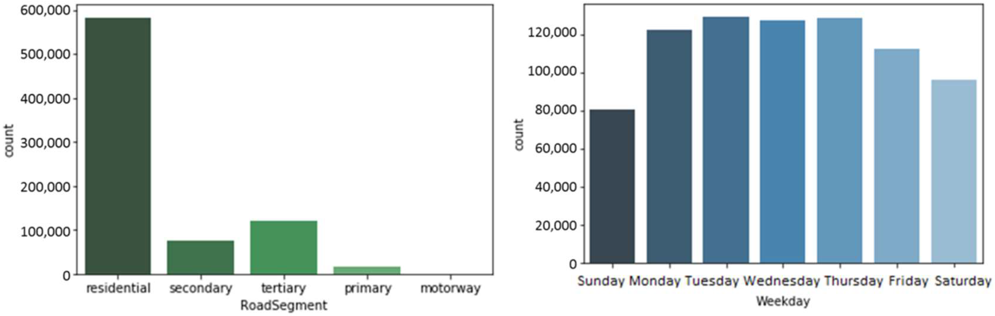
Figure 1 shows how the charging sessions on the dataset analyzed are split across the road segments (left) and weekdays (right). The high share of 74.1% of charging sessions in the residential road segment is mostly explained by the higher number of residential segment chargers overall accounting for 67.8% of connectors followed by tertiary with 15.5% and secondary with 9.58% [7]. Furthermore, it is typically the public charging solution used by users when they are at home. In motorways the share is negligible since the chargers typically installed in this road segment are fast chargers.

Regarding the distribution by days of the week, Figure 1 (right) shows a clear distinction between the number of observations during week days and weekends. Tuesdays and Thursdays are the days where most sessions occurred, whereas Sundays registered the least number of observations approximately 28% less from the maximum.

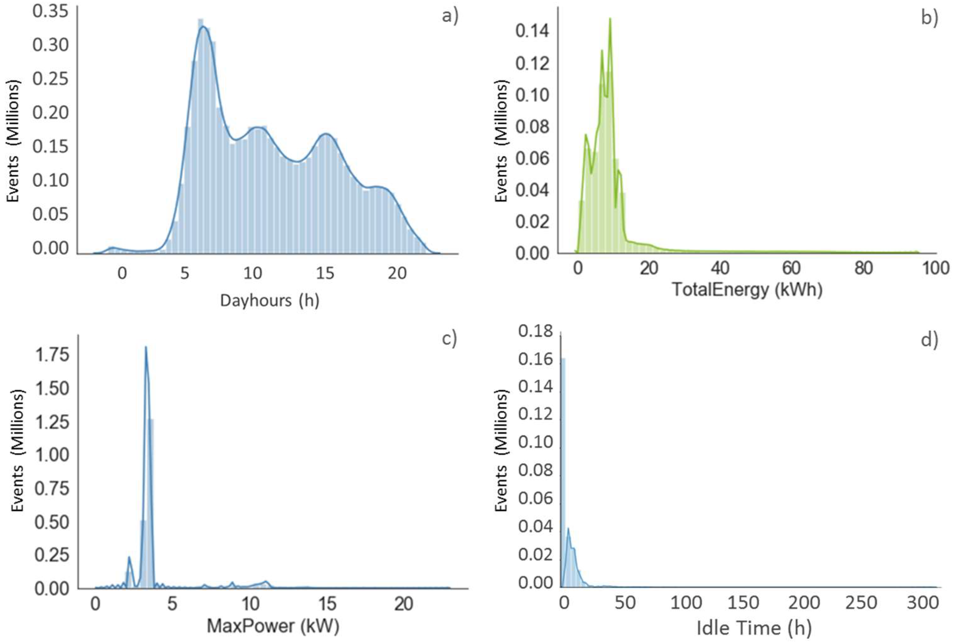
Figure 2 provides insights on the frequency of occurrence of sessions divided by the intraday hours, total energy, power supplied and idle time. Regarding the time of day (Figure 2a) there are three peaks where most sessions occur start. The first and highest occurs just after 8:00 a.m., the second around 11:30 and the third 16:30 which fit usual business routine hours, where users start and finish their charging sessions. It can also be seen from the energy histogram (Figure 2b) that most sessions charge up to 17 kWh (mean of 8.37 kWh), which, considering that most vehicles, until now, have had batteries up to 24 kWh, would mean up to 70% of charging (mean of 37%). Taxis and higher capacity battery pack vehicles, such as Tesla, may be responsible for the remaining tail observations. With a tendency of vehicles to increase their battery capacity to 40 kWh and higher, a wider distribution or a shift in the total energy supplied during the sessions can be expected in the histogram. The power histogram in Figure 2c shows that most sessions use on average of 3.8 kW of power supply. Figure 2d shows the complete range of idle time in the data set with extremely high values close to 300 h. However, the right skewed histogram shows a median value below 8 h.

The authors of Reference [7], having analyzed the data set for the years 2014 and 2015, report that the mean availability of the public charging infrastructure depending on the time of the day may vary from 37.8 to 99.8%. The mean idle time assessed in their study represented about 64.1% of the connected time. This value is coherent with the updated dataset of the present study which shows an idle time mean of 62.3% of the connected time. The lack of an available charger means that an EV user must approach the next available charger/connector, which may not always be close or easily reachable.

Table 1. Nearest neighbor (NN) average distances to connector based on Reference [7].

Road Segment	Mean NN Charger Distance (m)	Mean NN Connector Distance (m)	Min. (m) Distance	Max. (m) Distance
Primary	15,565	9462	3.1	52,900
Residential	1838	1101	1.78	21,910
Secondary	6359	3985	1.73	30,593
Tertiary	4872	2850	6.99	27,382
Total	1603	968	1.73	12,087

presents the nearest neighbor distances by road segment, showing the direct line average distances that an EV user would have to travel to approach the next potential available charger, within the Elaad infrastructure.

3.2. Data Treatment and Algorithms

The main tools used in this study for data processing and developing the models are R studios and Python. Scikit-learn [24] is the machine learning library used for RF and GB, containing a vast range of options for classification and regression models and well accepted in the scientific community. XGBoost uses a different source but it can be called both in R and Python as well [25].

Some manipulation of the data was carried out in order to prepare it for running the algorithms. The null value lines have been removed, as well as correlated or non-useful attributes (Index, Connected Time, Transaction Id, UTC Transaction Start, UTC Transaction Stop, Meter Start, Meter Stop, Stop Card, Latitude, and Longitude) reducing the dataset to 1.5 million observations. Furthermore, the original dataset presents an idle time range of 0 to 299 h. The intended output of the model is of continuous nature providing estimations also in hours. Due to the large range of times, it would be very unlikely to have a model which could be trained to estimate the idle time with acceptable accuracy. 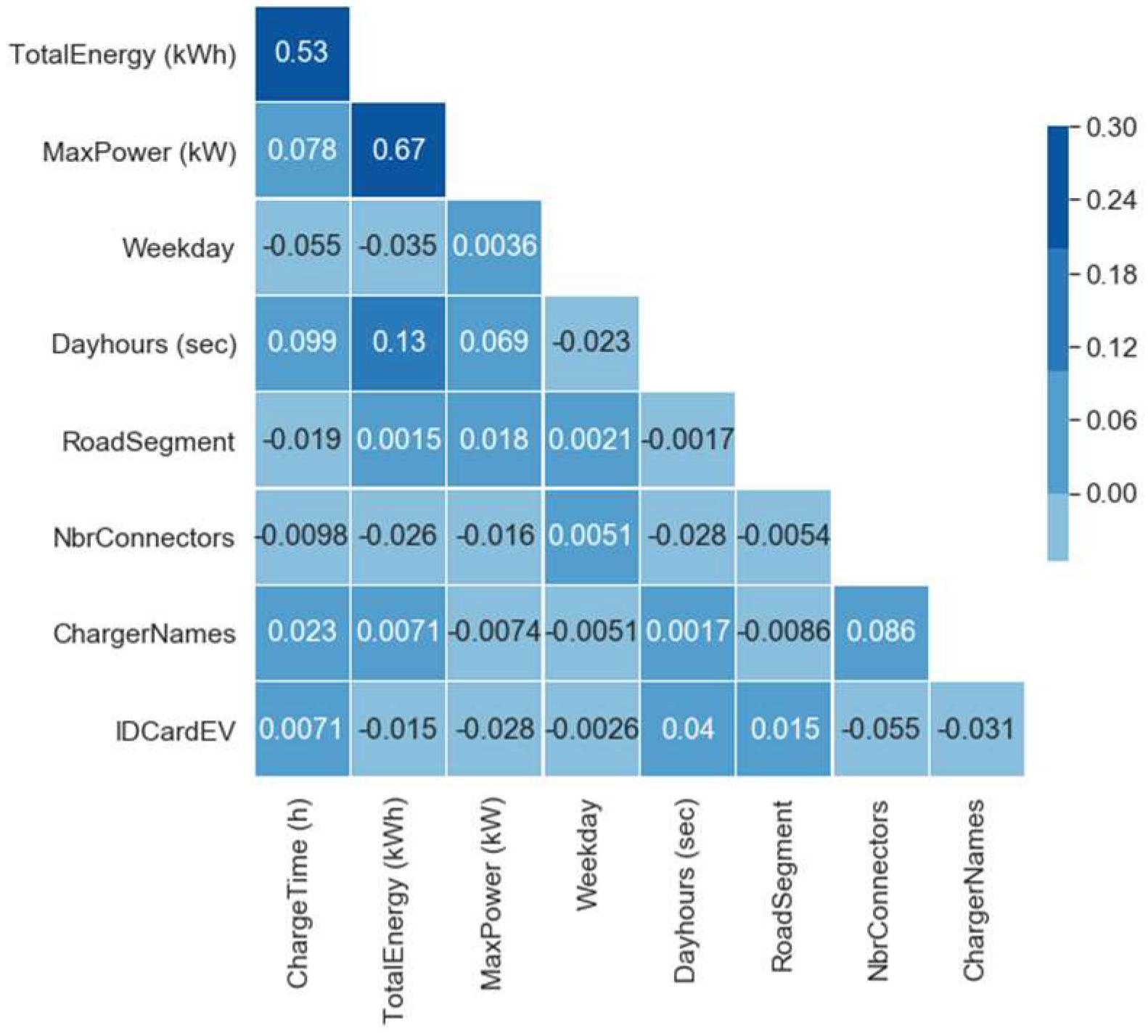As addressed in the literature [12], time windows should be considered and studied individually. For this reason, only idle times below 8 h are considered which adding to the mean charge time still means the majority of observations (1.1 million). In addition to this, to ensure that trial connections, short charges or error connections are not included, only charges above 15 min, which corresponds on average to approximately 1 kWh, are included in the analysis, resulting in 0.93 million observations. In terms of timespan only sessions between 31st December 2013 and 30th June 2018 are considered, meaning 0.73 million observations. The resulting dataset is composed of nine variables, including four numeric ones: Charge time, total energy, max. power, day hours (which refer to the the intraday hours of day) and five categorical: Road Segment, Nbr. Connectors, Charger Names, ID Card EV and Weekday. To check for variable independence a correlation matrix was generated and can be seen in Figure 3. The matrix confronts all variables to each other and checks for correlations, displaying the corresponding value in the intersecting box. Darker blue boxes have higher correlation than light blue ones.

The highest correlation is positive and observed to be 67% between max. power and total energy variables. The second highest correlation of 53% is also positive and observed between charge time and total energy. They are both however below 70% and hence considered as moderately correlated. Given these relations it is worth noticing however that max. power and charge time variables have only 7.8% correlation, since a higher power supply does not necessarily mean that the charge time would be reduced. This can only be explained by the fact that more energy is supplied as it is confirmed by the highest correlation. There is also a 13% correlation between day hours and total energy variables, which even though of low significance, hints that there might be preferred day times by EV users.

The dataset contained extremely high values especially in charge time variable, where it returned a maximum value of 245 h. In order to avoid outliers from potential mismeasurements, the dataset was limited to the percentiles between 2% and 98%. After data treatment, cleaning and considerations the final dataset was composed of 733,477 observations which correspond to 63,383 different EV users which we assume to be unique start cards values for this categorical variable. Other categorical variables have the following unique variables: Connectors 1 or 2, road segments has five categories (primary, secondary, tertiary, residential, motorway) and weekday has seven categories corresponding to the days of the week.

Table 2. Dataset summary of numeric and target variable considered (before scaling or test split).

Parameter	Charge Time (h)	Idle Time (h)	Total Energy (kWh)	Max. Power (kW)
min	0.6200	0.0003	0.1000	0.119
25%	1.750	0.531	5.290	3.248
Std.	1.028	2.410	6.181	1.857
mean	2.577	2.606	8.382	3.795
count	733,477	733,477	733,477	733,477
50%	2.500	1.740	7.611	3.380
75%	3.491	4.580	9.641	3.548
max	5.749	8.000	76.370	22.800

presents the summary for the numeric variables. The order of magnitude is the same as can be seen by the mean and neither minimum nor maximum values appear to contain outliers.

In order to train the algorithms using the dataset all variables should be converted into a numeric form. This means that category variables, such as road segment or weekday, have to be transformed into a numeric form. Numerical and categorical variables (in this case nominal) are pretreated using the Standard Scaler and One Hot encoder functions respectively. The Standard Scaler feature is used for numeric variables, which scales the different values of different magnitudes and places them all under the same reference range. Centering and scaling happen independently on each feature. This happens by processing the relevant statistics on the samples in the training set. The mean values and standard deviations are then kept in memory to be used on later data, using the transform method. The standardization technique of a dataset is a commonly used in many machine learning estimators, particularly if the orders of magnitude widely differ. The reason for this is that they might underperform if the individual features do not tend to follow a normally distributed data pattern. In this procedure, the center value is placed around zero and the range is typically set to between −1 and 1.

Regarding the categorical variables, they can be divided into two different types: Nominal and ordinal. The first group may refer to a variable describing a road segment, which when replaced by numbers ex: Motorway by 3, Primary by 2 and Tertiary by 1, does not mean that the Motorway road segment is higher than the Primary one. Furthermore, the model may make an assumption that Tertiary plus Primary is equal to Motorway, which is not correct. Concerning the ordinal type, this category may refer to a size ex—low, medium and high. When replacing this last group by numbers 1, 2, 3 respectively, this is label encoding and it could be correct to consider 3 higher than 1, hence no further transformation may be required.

When label encoding the categorical variables is not enough or desirable, a popular methodology followed is one-hot encoding. A one-hot encoder maps a column of category indices and transforms the categories into variables. These variables will then typically assume the value of 1 or 0 per each line or observation, depending on if such variable was a former category of that same observation.

The RF and the GB algorithms even though capable of working with classes, they have to be numeric strings at least. Therefore, five variables are described as objects or classes, day hours as integer (int64), and time, total energy and max. power, as float (float64) types. XGBoost does not work with objects, so both approaches of converting to numeric and one-hot encoding were used for the categorical variables. The float variables are maintained and the remaining considered as integers (int64). Both approaches were compared to this model, and no significant variation on the accuracy was observed by using the one-hot encoder method. Once the data treatment is finished the algorithms are run with a split ratio between training and test data with 80%–20% proportion respectively. With the initial results, the Hyperparameters are optimized for each algorithm and the number of estimators fine-tuned. In the end the models are run again to check for new accuracies in an iterative process, and in order to use most of the training data with 95%–5% split.

3.3. Model Accuracy Evaluation—Regression Metrics

R² is called the coefficient of determination, also known as regression score function. This score is estimated by comparing the target variable under test (y_test or idle time) to the prediction values of that target provided by the model. The best possible score for this coefficient is 1.0 and it can also provide a negative value, given that the model can be actually worse. A constant model that always predicts the expected value of y, disregarding the input features, would get an R² score of 0.0. R² will provide information on how close the model is in predicting the target variable and is particularly used in regression [26]. It is given by Equation (1), where the numerator is the sum of squares of residuals, divided by the total sum of squares (proportional to the variance of the data).

$$R^2=1-\frac{{\sum }_i{e}_i^2}{{\sum }_i{\left(y_i-\overline{y}\right)}^2}$$

(1)

Root Mean Square Error (RMSE) measures the standard deviation of the residuals (prediction errors). Residuals are a measure of how far from the regression line data points are, it can be seen as a measure of how spread out these residuals are. It provides information on how concentrated the data is around the line of best fit. Root mean square error is commonly used in climatology, forecasting, and regression analysis to verify experimental results and is given by Equation (2), where f are the forecasts (expected values or unknown results) and o the observed values (known results).

$$\mathrm{RMSE}=\sqrt{\overline{{\left(f-o\right)}^2}}$$

(2)

Mean Absolute Error (MAE) estimates the average magnitude of the errors in a set of predictions provided by a model, without considering their direction. In other words, it computes the average of the absolute differences between prediction and actual observation of a given test sample considering that all individual differences have equal weight [27]. It is important to distinguish two concepts: The “standard error” of the sample mean provides an estimate of how far the sample mean is likely to be from the population mean. A second concept is the standard deviation of the sample which provides the degree to which individuals within the sample differ from the sample mean. Even though the MAE is not the standard deviation is can be a good estimation to understand if the model improves traditional statistics approach or not. The MAE can be calculated by Equation (3) [27].

$$\mathrm{MAE}=\frac{{\sum }_{i=1}^n\left|e_i\right|}{n}$$

(3)

4. Results and Discussion

To optimize hyperparameters there are two popular methods of approaching it: Randomized Parameter Optimization and Grid search (Grid search CV). The randomized search and the grid search methods explore exactly the same space of parameters. The result in parameter settings is rather identical, while the run time for randomized search when compared to grid search is drastically lower. The randomized search approach performs worse, though this is most likely due to noise effect. In practice, one would not search over this many different parameters simultaneously using grid search, but pick only the ones deemed most important. In this study we have used Randomized Parameter Optimization, which is the randomized search CV method provided by the scikit-learn [21] library. The Hyperparameter tuning is an intensive optimization problem which can take several hours. Two main parameters have to be input for this exercise to be carried out and which determine its accuracy and time: The number of iterations (N_iter) and the Cross Validation (CV). N_iter is the number of parameter settings that are sampled, trading off runtime. The CV determines the cross-validation splitting strategy (for example 3 folds), which controls the model from over fitting. One multiplied by the other will provide the number of fits. In this study n_iter:50 (candidates) and CV:3 (folds) were used corresponding to 150 combination/fits. All optimized hyperparameters are presented in

Table 3. HyperParameters used in each method.

Methods	HyperParameters
RandomForrest	{‘n_estimators’: 2000, ‘min_samples_split’: 7, ‘min_samples_leaf’: 2,’max_features’: ‘sqrt’, ‘max_depth’: 63, ‘bootstrap’: True}
GradientBoosting	{‘learning_rate’: 0.1, ‘max_depth’: 15, “min_samples_leaf”: 2,’min_samples_split’: 10, ‘n_estimators’: 542, ‘subsample’: 0.8}
XGBossting	{‘subsample’: 0.8, ‘seed’: 421, ‘n_estimators’: 2750, ‘min_child_weight’: 5, ‘max_depth’: 9, ‘colsample_bytree’: 0.9}

according to each method used.

It can be observed that even though RF and XGBoost have close number of trees, GB is optimized with 542. It does not mean however, that GB is processed faster than the others; in fact, it was quite the opposite. Moreover, the max_depth in RF is 63 while GB and XGBoost are within the same order of magnitude with 10 and 9 respectively.

Table 4. Model Performance comparison between methods.

Methods/Metrics	R2 (%)	Mean Absolute Score	Root Mean Squared Error
Random Forrest	56.33	1.20	1.59
Gradient Boosting	59.08	1.13	1.54
XGBoost	60.32	1. 11	1.51

shows the results for the metrics assessed by each model. The XGBoost was the one with the highest R² score of 60.32%, which also obtained the lowest mean absolute score of 1.11. Instead Gradient Boosting achieved accuracy close to the highest value with 59.08% and RF 56.33. Different factors may influence the training time, such as processing capacity or operating system, however under the same conditions (PC with 64 GB RAM), it was observed that GB took approximately 7 h to train the model, whereas RF took 1 h and XGBoost 40 min.

Figure 4 shows a visual representation of how an XGBoost decision tree processed by the model looks like, showing the features and feature values for each split, as well as the output leaf nodes. It is possible to see the split decisions within each node and the different colors for left and right splits (blue and red). For the sake of presenting an example, Figure 5 only presents the first tree with a max_depth = 3 (circular layers) instead of 9 as determined in the Hyperparameters. The n_estimators is the number of regression trees ran by the model, which are a variation of the simple representation shown.

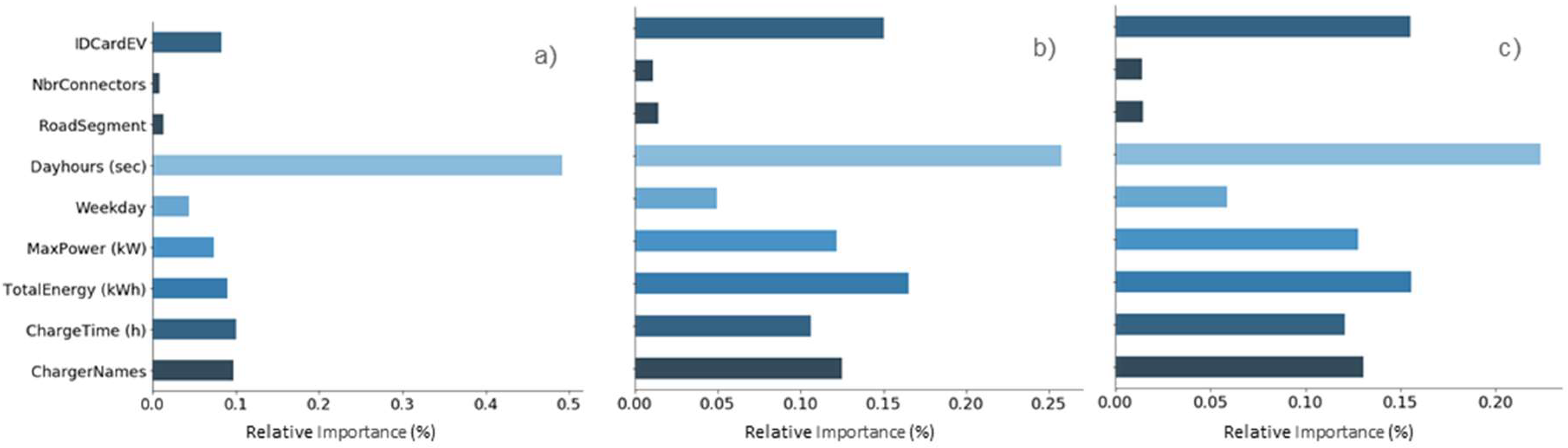
Having obtained the accuracies, all models are able to provide the feature importance, shown in Figure 5, which is the impact or weight that each variable has in predicting the target variable. From the outcome it can be understood the different approaches followed by each model in taking into account the variables. The RF model results shown in Figure 5a, emphasizes the weight of the most impactful variable which is the daytime, whereas the boosting approach, seen in the GB Figure 5b, emphasizes the iterative functional gradient descent approach, resulting in a weight distribution among variables. Finally, in Figure 5c XGBoost reveals the attention it provides to considering the possible loss for potential splits to create a new branch in a tree. This may be a possible explanation to why the contribution in this model is more diverse than in RF.

Even though with different weights, all models tend to point out the same variables as being the most impactful ones. day hours, total energy charged, time, max. power and ID Card EV are the top 5 features. Results are consistent with what is reported in the literature [12], especially regarding connection times of EVs to charging stations and to be dependent on time-of-day related variables. The ID Card EV holders is an anticipated high impactful variable, since EV user’s behavior is expected to be consistent with routines/human nature. The Charger Name feature probably includes location specific characteristics that might play an important role, justifying its importance.

Despite informing about the weight of each variable, the feature importance analysis cannot clarify if the impact of each variable is negative or positive. For this reason an analysis on partial dependencies is carried out, where the impact of one variable is observed, while the remaining variables maintain a constant mean value [28]. XGBoost library does not provide this feature of analysis so a script following a similar approach was developed. Figure 6 presents the most significant results for XGBoost as an example. The partial dependence is in hours and it refers to idle time estimated.

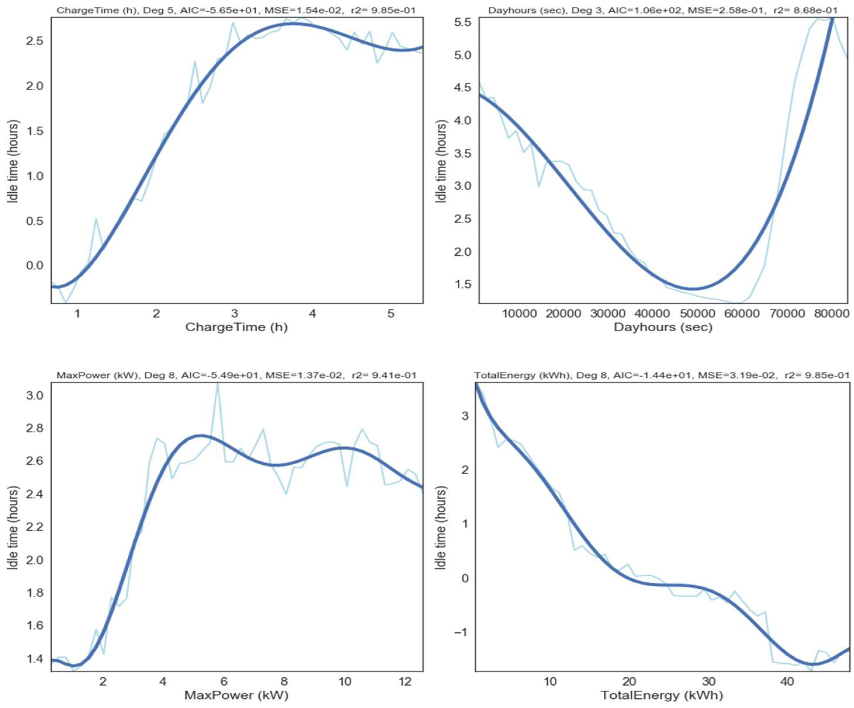
To determine a possible impact on Idle Time from each individual contribution as a function of a given x, Equations (4)–(7) may be used. These functions are derived from the corresponding polynomial trend curves also presented in Figure 7. The degree for the polynomial functions is determined by the Akaike information criterion (AIC) [29]. AIC provides an output degree considering the trade-off between the goodness of fit of the model and its simplicity.

$$\begin{array}{c}{y}_{\text{Max.Power}}=1.3339+0.3694\mathrm{X}-0.8133{\mathrm{X}}^2+0.6239{\mathrm{X}}^3-0.1921{\mathrm{X}}^4+0.0299{\mathrm{X}}^5-\\ 0.0025{\mathrm{X}}^6+0.0001{\mathrm{X}}^7-1.9033e^{-06}{\mathrm{X}}^8\end{array}$$

(4)

$$y_{\mathrm{Charge}\mathrm{Time}}=0.9105-3.6110\mathrm{X}+3.42586{\mathrm{X}}^2-0.9728{\mathrm{X}}^3+0.1065{\mathrm{X}}^4-0.0035{\mathrm{X}}^5$$

(5)

$$\begin{array}{c}{y}_{\mathrm{Total}\mathrm{Energy}}=3.8667-0.5682\mathrm{X}+0.1084{\mathrm{X}}^2+-0.0133{\mathrm{X}}^3+0.0008{\mathrm{X}}^4-2.4695e^{-05}{\mathrm{X}}^5+\\ 3.8338e^{-07}{\mathrm{X}}^6-2.5677e^{-09}{\mathrm{X}}^7+3.6259e^{-12}{\mathrm{X}}^8\end{array}$$

(6)

$$y_{\mathrm{Day}\mathrm{hours}}=4.4199-3.3644e^{-05}\mathrm{X}-2.3955e^{-09}{\mathrm{X}}^2+3.7332e^{-14}{\mathrm{X}}^3$$

(7)

The direction of the contributions varies immensely and provides good insights on where to focus, if idle time needs to be managed. It can be seen that higher charging times from 6 h on, has a positive and higher impact on the idle time prediction than lower charging times. This can be explained by the fact that users do not stay near the vehicle and engage on some other activity (ex—work), while leaving the car charging. This often results in connection times surpassing greatly the charge time. The total energy on the other hand seam to impact more on the target estimation when lower values are observed, possibly because the total connection time will be closer to the charge time itself. Although the trend of the level of power supply on the idle time is not very well defined, it can be seen that higher rates of power (>3 kW) contribute more than lower levels. Moreover, the intraday time is the one where higher contribution is verified. The highest impact on the values of the predicted idle time is observed to start from 17 h (61,200 s) onwards which coincides when EV users arrive home and charging sessions may start then, lasting for the whole night or part of it. Charging sessions which start around 14 h (50,400 s), appear to have less impact in the idle time prediction.

Table 5. Comparison between Y-test and Model Prediction.

	Prediction XGBoost	Prediction GB	Prediction RF	y Test
Std. Dev	1.85	1.87	1.70	2.41
Mean	2.58	2.61	2.60	2.61
Maximum	8.55	8.47	7.7	8.00

presents the statistical description of the prediction model. Even though RF has a smaller standard deviation of 1.70 when compared to the y test set, it is not the model with the highest accuracy. This depends on the sampling of the data used, which is different every time, and it should not be confused as a closed comparable indicator among model’s results.

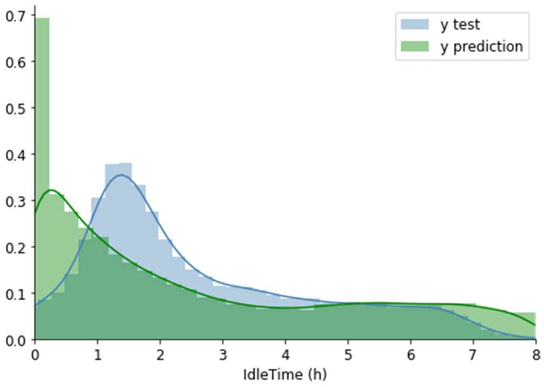
Such an analysis is only used for a given test and prediction run. If one needs to estimate every value of Y but knows nothing about Y, except that it has a mean of let’s say 2.61 h, then one should guess 2.61 h every time. It would be wrong most of the time (a lot, considering that in this case the standard deviation is 2.41 h), but pursuing other strategies can result in even larger errors, unless that error is found to be less. SD is always larger than (or rarely, equal to) the mean error. The model even though with satisfactory accuracy of 60.32% provides acceptable metric ratios, at least more robust than a simple SD from the y test, attesting the success of the model. The match between the XGBoost prediction and the y test set can be seen in Figure 7.

A word should be said about the inclusion or exclusion of variables in the models. Some approaches run the model in order to calculate feature importance and disregard the one(s) with very low relative contribution. This is usually done when the data analyst is willing to trade off accuracy for processing performance. Furthermore, it is important to mention that the model has to be able to incorporate updatable variables. In the case under study, this means that if for example new chargers were to be added to the existing network or if new EV card owners would start using the network for the first time, the model will not recognize them as inputs, as they are not part of the training dataset. Hence a mechanism has to be included for updatable variables to enable their inclusion, whenever a new record or set of records are detected. In other words, the model has to be re-trained often to account for changes in the variables.

The identification of impacting variables opens the door to action, depending on the goals towards Idle Time management. Public policies targeting time of day, charge time and total energy should be the most efficient ones considering the model’s outputs. As examples, policies defining the minimum amount of charge (or a minimum charging time) could be used for varying the Idle Time. Moreover, limiting free parking hours, would be yet another example of an action that could impact idle time. Policies could have different configurations depending on the road segments, cities or regions.

5. Conclusions

In this study the performance of Gradient Boosting, Random Forests, and XGBoost methods were compared for estimating the Idle Time (parked without charging) of an EV after the charging process occurs. The study, confirms that the Idle Time can indeed be estimated with a fair degree of accuracy for the dataset under study and presents the procedure which can be followed to different datasets from other regions or contexts. It provides useful information for users to perceive the availability of the charging infrastructure and plan its own use. It was observed that separation of time windows should be followed due to the high variability of Idle Times. The model can be a useful tool for EV users, to decide whether to wait or approach a different connector/charger. Furthermore, infrastructure owners and city/region management authorities may be able to target specific variables with public policies in order to reduce the total idle time, or make use of it by for example shifting demand. In this sense the variables identified in this study to impact the Idle Time the most were: Intraday hours and total energy supplied with 22.35%, 15.57% contribution respectively. Policies, such as requiring a minimum energy per charging session, restricting free parking in EV charging points in certain hours, or allowing such parking space to be used by other non-EV users or similar, could be options to be considered. Load scheduling, power reduction or complete load shifting, are options to make the most of Idle Time as it is, considering it as an opportunity for grid management.

From the comparison, XGBoost algorithm performed better in terms of the metrics analyzed. Its ability to mitigate overfitting scenarios contributes to its higher success in predicting new data. It returned a coefficient of determination (R²) of 60.32%, Root Mean Square Error (RMSE) of 1.51 and a Mean absolute error of 1.11. As the dataset grows the training, optimization and prediction time may increase substantially. Updating the model by sampling could be an option to mitigate this potential problem with an accuracy trade off.