Numerical Analysis of Transient Pressure Behaviors with Shale Gas MFHWs Interference


1
State Key Laboratory of Oil and Gas Reservoir Geology and Exploitation, Southwest Petroleum University, Chengdu 610500, China
2
Institute of Mechanics, Chinese Academy of Sciences, Beijing 100190, China
3
School of Engineering Science, University of Chinese Academy of Sciences, Beijing 100049, China
4
Beijing International Center for Gas Hydrate, Peking University, Beijing 100871, China
*
Authors to whom correspondence should be addressed.
Energies 2019, 12(2), 262; https://doi.org/10.3390/en12020262
Submission received: 6 November 2018
/
Revised: 8 January 2019
/
Accepted: 9 January 2019
/
Published: 15 January 2019
(This article belongs to the Special Issue Development of Unconventional Reservoirs)
Abstract
:After the large-scale horizontal well pattern development in shale gas fields, the problem of fast pressure drop and gas well abandonment caused by well interference becomes more serious. It is urgent to understand the downhole transient pressure and flow characteristics of multi-stage fracturing horizontal well (MFHW) with interference. Therefore, the reservoir around the MFHW is divided into three regions: fracturing fracture, Stimulated reservoir volume (SRV), and unmodified matrix. Then, multi-region coupled flow model is established according to reservoir physical property and flow mechanism of each part. The model is numerically solved using the perpendicular bisection (PEBI) grids and the finite volume method. The accuracy of the model is verified by analyzing the measured pressure recovery data of one practical shale gas well and fitting the monitoring data of the later production pressure. Finally, this model is used to analyze the effects of factors, such as hydraulic fractures’ connectivity, well distance, the number of neighboring wells and well pattern arrangement, on the transient pressure and seepage characteristics of the well. The study shows that the pressure recovery double logarithmic curves fall in later part when the well is disturbed by a neighboring production well. The earlier and more severe the interference, the sooner the curve falls off and the larger the amplitude shows. If the well distance is closer, and if there are more neighboring wells and interconnected corresponding fracturing segments, the more severe interference appears among the wells. Moreover, the well interference may still exist even without interlinked fractures or SRV. Especially, severe interference will affect production when the hydraulic fractures are connected directly, and the interference is weaker when only SRV induced fracture network combined between wells, which is beneficial to production sometimes. When severe well interference occurs, periodic well shut-in is needed to help restore the reservoir pressure and output capacity. In the meanwhile, the daily output should be controlled reasonably to prolong the stable production time. This research will help to understand the impact of well interference to gas production, and to optimize the well spacing and achieve satisfied performance.
1. Introduction
The multi-stage fracturing horizontal well (MFHW) is a crucial technology in shale gas development, and the large-scale horizontal wells pattern haves achieved remarkable performance in many fields in North America and China [1,2,3,4,5]. However, some well groups have shown increasingly dangerous well interference after producing for several years, due to the well pattern infilling and enhancement of hydraulic fracturing. For instance, The Jiaoshiba shale gas play is the most successful shale gas reservoir in China with some wells’ cumulative production over 0.1 billion cubic meters in the first year; unfortunately, parent wells crop up jumps in water production during hydraulic fracturing processing of child wells in the later production period. Besides, North American shale plays, such as Arkoma Basin, have also shown an obvious loss of gas production because of well interference [6,7]. Fracture pressure hits and production interference are two main factors influencing the shale gas permanent development and determining the inter-well connectivity [8].
By a combination of hydraulic fracturing process and production data, the existence of well interference from the adjacent wells when well interference happens and the influence it imposes on the target well can be detected. Maintaining a high and stable gas productivity faces many challenges in the future. It is urgent to study in depth the transient pressure behaviors of shale gas MFHWs with neighboring wells, considering the complex fracture network and the multi-flow mechanism, such as the desorption and diffusion of shale gas [9,10], to recognize the well interference in time and analyze its impact on production. Mezghani et al. [11] combined gradual deformation and upscaling techniques for direct conditioning of fine-scale reservoir models to interference test data, as consequence, both fine- and coarse-scale models are updated by dynamic data during the history matching process. Yaich et al. [12] presented a methodology to quantify the impact of well interference and optimize well spacing in the Marcellus shale. Marongiu-Porcu et al. [13] proposed a numerical simulation method for shale gas reservoirs based on geophysical, completion and development data of Eagle Ford shale gas fields, and studied the propagation of hydraulic fractures and their respective network with natural fractures. The magnitude and orientation of in-situ stress were evaluated. Pang et al. [14] studied the effect of well interference on shale gas well SRV interpretation. Compared with the previous literature, we analyzed the interference using the numerical simulation pressure double logarithmic curve method and evaluated the influence of various factors on the interference.
To study the porous media flow and transient pressure behaviors of shale gas MFHWs, many scholars have established kinds of multi-linear flow region coupled models. Bello et al. [15] used the layered double porosity model and the Warren-Root dual-porosity model to analyze the pressure response and production dynamics of multi-stage fracturing horizontal wells in shale reservoirs. Ozkan [16] and Al-Rbeawi [17] divided the stimulated shale reservoirs into hydraulic fractures, stimulated reservoir volume (SRV), and matrix. Moreover, they simplify the flow in these three regions into the one-dimensional linear flow by establishing a three-linear-flow model. Additionally, Stalgorova [18] and Zhang et al. [19] improved the three-linear-flow model by considering the un-stimulated areas between two hydraulic fracturing SRV and proposed a five-region coupled flow model. Zeng et al. [20] further subdivided the five-region coupled flow model and proposed a seven-region coupled flow model. Based on these coupled models, Wang et al. [21] and Kim et al. [22] analyzed the stress-sensitive effects of gas reservoirs and fractures. Overall, the flow around shale MFHWs is mainly characterized by coupled linear flow models with multiple subdivided regions. In these models, hydraulic fracture (HF), SRV, and matrix are commonly applied, and they are separately discussed as follows. The flow in fracturing fractures usually satisfied Darcy law or high-speed non-Darcy law [23]. The SRV can be treated as dual media, or characterized by complex fracture network models [24]. The matrix can be regarded as a homogenous ultra-low-permeability medium. However, some scholars treat it as a dual medium with natural fracture network [25]. The equivalent permeability can be analyzed in the multiple regions coupled model to simplify the effects of desorption and diffusion in the SRV and matrix. From these three main regions, five regions or seven regions are further subdivided, but the physical parameters in the added regions are difficult to obtain. Well interference may be caused by interaction between primary hydraulic fractures and/or secondary natural fractures activated during hydraulic fracturing. Well interference has had a significant influence on the SRV interpretation. Well interference has drawn people’s attention in recent years, but its impact on transient behaviors is rarely reported.
As shown in the previous literatures, Laplace transform and Stehfest method are mainly applied to obtain the analytical solution or semi-analytical solution of transient pressure behaviors. It is principally applicable for the analysis of one single shale gas well, but it’s really difficult to solve the transient pressure with multiple well interferences. So it’s crucial to investigate a numerical method to analyze the well pattern pressure dynamic. Therefore, to fully understand the transient pressure behaviors with well interference, a three-medium coupled numerical model is given in the paper, considering connected and unconnected HFs, SRV, and matrix. Also, we numerically solve the model by PEBI grids and the finite volume method. Different factors’ influences on transient pressure behaviors with well interference are studied. This research may help to characterize well interference and related factors and to optimize well spacing.
2. Model Description
Due to the significant difference in porosity and permeability between the fracturing and un-fracturing areas in the reservoir, shale reservoirs around MFHWs are divided into sub-regions, including hydraulic fractures, SRV with abundant inducing micro-fractures, and matrix as shown in Figure 1. Among them, only SRV region is simplified as dual medium due to micro-fracture development; matrix region is single-porosity single-permeability medium, hydraulic fracture is a high permeability medium. Assumptions: (1) Water flow is ignored, and there is only single-phase gas flow existed in each sub-region. (2) Just viscous flow exists in the HF and satisfies the Darcy law [26], neglecting the longitudinal flow. (3) SRV is treated as dual media, and each hydraulic segment’s SRV overlaps with each other in one MFHW. (4) Matrix is regarded as homogeneous ultra-low permeability media. (5) Pseudo pressure function (m) is introduced to simplify the gas composition change with temperature and pressure [27]. (6) There are three connection modes between the well and its neighboring wells, including the connection of the inducing micro-fracture clusters in the SRV and the connection of hydraulic fractures as shown in Figure 1.
3. Mathematical Model
3.1. HF Flow Model
It is assumed that fluid exchanges exist among the fracture, the SRV and the wellbore, the boundary between the well and the HFs is defined as Γ1, and the boundary between the SRV and the HFs is Γ2. If the HFs directly connected in one well pair, the fluid exchange between two wells’ HFs needs to be considered. Commonly, shale gas wells produce at a given production rate first according to the development scheme, and the gas supply capacity of the reservoir gradually tends to insufficient as the pressure continues to drop. The shale gas wells are converted to produce with constant pressure later. Based on this, the flow equations in the finite conductivity fractures are established as follows:
The initial conditions:
Inner boundary condition:
Constant pressure boundary conditions:
Fixed output boundary conditions:
Outer boundary condition:
3.2. SRV Flow Model
SRV exist around MFHWs in unconventional shale reservoirs, which leads to the flow characteristics of the fluid that are different from those in unstimulated formations. It is necessary to integrate various measurements and surveillance data to build a variable SRV reservoir model. The variable SRV model described here has the following building blocks [28]: (1) Formation evaluation: included all the reservoir characterization data derived from logs and 3D seismic inversions and structural attributes. (2) Surveillance data integration: micro-seismic data are integrated with chemical and radioactive tracer logs. (3) Well performance data integration: Production data is used to determine different flow regimes during the well history and to set bounds for stimulation parameters, such as HF half-length and permeability. (4) Numerical simulation: Micro-seismic attributes (density and magnitude) are converted to a permeability model after being calibrated with tracer logs and production flow regime parameters. pressure, volume, temperature (PVT) data is matched against an Equation of State and input into the model. Due to the abundant micro-fractures induced by hydraulic fracturing in SRV, SRV is regarded as a dual medium containing the matrix and fracture systems.
(1) Matrix system flow model
Assuming that gas desorbed from the SRV matrix system, the desorption gas satisfies the Langmuir isothermal adsorption equation on the surface of the matrix bedrock. The migration of gas includes viscous flow, Knudsen diffusion, and surface diffusion. So, the matrix system flow model is Equation (2):
(2) Fracture system flow model
Because the micro-fractures in the SRV region are very developed, how to characterize the fracture network equivalently in the seepage model has been a difficult problem to solve. For this reason, many scholars hypothesize that the development and spread of fracture networks satisfy the fractal characteristics and propose a fractal model that characterizes natural fracture networks [29,30]. However, the critical parameters such as the fractal dimension in the model are difficult to determine. Also, considering complex networks will greatly increase the complexity of meshing and numerical calculations. Therefore, the equivalent permeability is used to characterize the comprehensive permeability of the fracture system in the SRV region. The gas in the fracture medium in the SRV is mainly in the form of free gas. Therefore, only the viscous gas flow and Knudsen diffusion are considered in the fracture medium, and the apparent permeability ks,f is used to represent the permeability of the fracture medium [31]:
Assume that the wellbore only has fluid exchange with the fracture, neglecting the direct fluid exchange between the fracture system and the wellbore in the SRV, and defining the interface between the fracture and the matrix systems in the SRV as Γ3. Then the flow model in the fracture system of the SRV is presented as Equation (4):
The initial conditions:
Inner boundary condition:
Outer boundary condition:
3.3. Matrix Flow Model
The shale gas reservoir is rich in kerogen organic matter, and the hydrocarbon gas generated in the kerogen satisfies the saturation adsorption and then spreads from the kerogen pores to the inorganic matrix pore space where the hydrocarbon concentration is relatively reduced. The gas in the kerogen occurs in two forms: free gas and adsorbed gas. The pores in the kerogen have the same order of magnitude as the gas molecules in the shale gas. Therefore, the free gas will generate Knudsen Diffusion in the kerogen nanoporous network. At the same time, the kerogen is saturated with a large amount of adsorbed gas, and the adsorbed gas on the surface of the skeleton will produce surface diffusion. Assuming that the shale gas reservoir is isothermally developed, the Langmuir isotherm adsorption equation is used to describe the adsorption and desorption of kerogen.
The apparent permeability of the unmodified Matrix region proposed by Singh et al. [32] and Civan et al. [29,30] is:
Thus, the kerogen-medium continuity equation considering Knudsen diffusion, adsorption-desorption and surface diffusion is obtained as Equation (6):
The initial conditions:
Inner boundary condition:
Outer boundary condition:
3.4. Model Solution
Accuracy and efficiency of reservoir simulators in complex systems depend highly upon a proper grid selection. Grids based on a cartesian coordinate system have been widely used, but have some disadvantages: (a) Flexibility in the description of faults, pinchouts, hydraulic fractures, horizontal wells and general discontinuities presented in reservoirs; (b) inflexibility in representing well locations; and (c) suffer from grid orientation effects. PEBI grids have been applied to the oil industry for about a decade. On the other hand, generation and construction of PEBI grids are not as easy as cartesian grids. The construction of PEBI grids for a reservoir is feasible only if it is done by a numerical grid generation procedure. These PEBI grids are locally orthogonal. It means the block boundaries are normal to lines joining the nodes on the two sides of each boundary. This allows a reasonable accurate computation of inter-block transmissibility for heterogeneous but isotropic permeability distribution.
The irregular geologic body boundary can be depicted by PEBI grids. In this paper, the unstructured PEBI grid is applied to mesh the solution area and carry on local grid refinement around MFHWs, in which the connection between the center node of each grid and the adjacent grid center node is perpendicular to the interface, as shown in Figure 2.
Finding a pressure solution for large-scale reservoirs that takes into account fine-scale heterogeneities can be very computationally intensive. One way of reducing the workload is to employ multi-scale methods that capture local geological variations using a set of reusable basis functions. One of these methods, the multi-scale finite-volume (MsFV) method is well studied for 2D Cartesian grids, but has not been implemented for stratigraphic and unstructured grids with faults in 3D. With reservoirs and other geological structures spanning several kilometers, running simulations on the meter scale can be prohibitively expensive in terms of time and hardware requirements. Multiscale methods are a possible solution to this problem, and extending the MsFV method to realistic grids is a step on the way towards fast and accurate solutions for large-scale reservoirs.
Moyner and Lie [33] presented an MsFV solver along with a coarse partitioning algorithm that can handle stratigraphic grids with faults and wells. The solver is an alternative to traditional upscaling methods, but can also be used for accelerating fine-scale simulations. In this paper, we use MsFV to discretize the reservoir area into non-overlapping control volumes, and each center node has a controlled volume around it. According to the seepage equation and boundary conditions of multiple composite flow models, the partial differential equations to be solved are integrated for each control volume, and a set of discrete equations is obtained.
Based on the flow control Equation (1) in the fracturing fracture, the control volume V of this point mesh is integrated to obtain Equation (7):
Use the Gaussian formula to convert the volume fraction of the left-side diffusion term of Equation (7) into area fractions, as Equations (8) and (9):
Assuming that the difference between the two time steps is Δt and the distance between the two neighboring grid center nodes is L, then the discrete Equation (9) can be converted to Equation (10):
Based on this, the discrete equations for the SRV and matrix area can be further deduced. The discrete flow equation for the SRV region matrix system is shown in Equation (11):
The discrete flow equation for the fracture system in the SRV region is shown in Equation (12):
Discrete flow equation in matrix can be expressed as Equation (13):
4. Results and Discussion
4.1. Model Verification
Taking the A1 well group in Chinese Jiaoshiba shale gas field for instance, we use the multi-region coupled model to analyze MFHWs’ transient pressure recovery behaviors during the shut-in process. In this shale gas field, the gas investigated permeability is 200–300 nD, porosity is 3%, and the reservoir thickness is approximately 90 m. Well A1-1 (in A1 well group) has operated 15 segments of hydraulic fracturing and put into production from April 2014. The average daily gas production was 6 × 10⁴ m3/d up to March 2018. In the same layer, there is an adjacent A1-2 well 300 m away from well A1-1. A1-2 has operated 19 segments of hydraulic fracturing and put into production from May 2014. Up to March 2018, its average daily gas production was 10 × 104 m3/d. The interpretation of the micro-seismic monitoring results shows that the two wells have partial overlap in the hydraulic fracture network. Therefore, it is preliminarily judged that the well communicates with the adjacent well through the SRV and HFs. In order to understand the reservoir parameters around the A1-1 well and its connectivity with the neighboring well A1-2, a pressure build-up well test was conducted during the production process of well A1-1, and the gas production of the neighboring well was maintained at 10 × 104 m3/d.
According to the pressure recovery test data of Well A1-1, the logarithm curve of the pseudo pressure and its derivative are plotted. It is found that the derivative curve dropped significantly in the last part, and it was initially judged that the well A1-2 is more severely interfered by well A1-1. Based on the spatial relationship of the two wells and the characteristics of the hydraulic fracture network, a numerical seepage model was established under the mode of ‘HF + SRV connection’, and the permeability and wellbore storage were obtained by fitting the pseudo pressure and its derivative curve (Figure 3). As shown in the Figure 3, the early time data is related to wellbore storage capacity, the early bulge data is related to skin effect, the middle time data reflects linear flow under fracture interference, this part would control fracture half-length, fracture conductivity and fracture spacing. The equivalent permeability of the SRV fracture system is 0.0507 mD, which is far greater than the permeability of the matrix (200–300 nD), and the ratio of horizontal to vertical permeability is only 0.0252, reflecting the general characteristics of shale reservoirs with low vertical permeability. SRV permeability is calculated by fitting pressure data. The average HF half-length of the two wells has reached about 100 m, and the HFs in the toe connecting section are as long as about 170 m. In order to verify the reliability of the model and the parameters, these parameters explained by the pressure recovery test data were assigned to the well group geological model, and the bottomhole pressure (BHP) changes in the later production process of the well were simulated (Figure 4). The comparison error with the BHP monitoring data is quite small.
4.2. Mechanism Model
The transient pressure behavior under well interference is influenced by various factors, such as the inter-well communication mode (IWCM), well spacing, number of neighboring wells, and well pattern arrangement [34,35]. The influence of different factors is analyzed by combining the established multi-zone coupled flow model. According to the reservoir and fracture parameters obtained from the well test and laboratory test data of Jiaoshiba shale gas field, it is assumed that the permeability of the matrix is 0.001 mD to 0.003 mD, and the SRV has a permeability of 50 to 200 times that of the matrix. The horizontal well-length is 1500 m. Each well is fractured by 19 sections, and except for connecting HFs, other HFs are of the same length and have the same conductivity; the initial pressure of the reservoir is 34 MPa, the temperature is 96 °C., and the gas component is dominated by methane (98%) with a small amount of nitrogen (0.7%), carbon dioxide (0.6%), ethane (0.4%), and propane (0.3%); the well spacing between the well and neighboring well is 300–600 m. Based on these parameters, a corresponding mechanism model was established. The well pair sketch and meshing grids under the coexistence conditions are shown in Figure 5.
4.3. Effect of Inter-Well Connection Mode
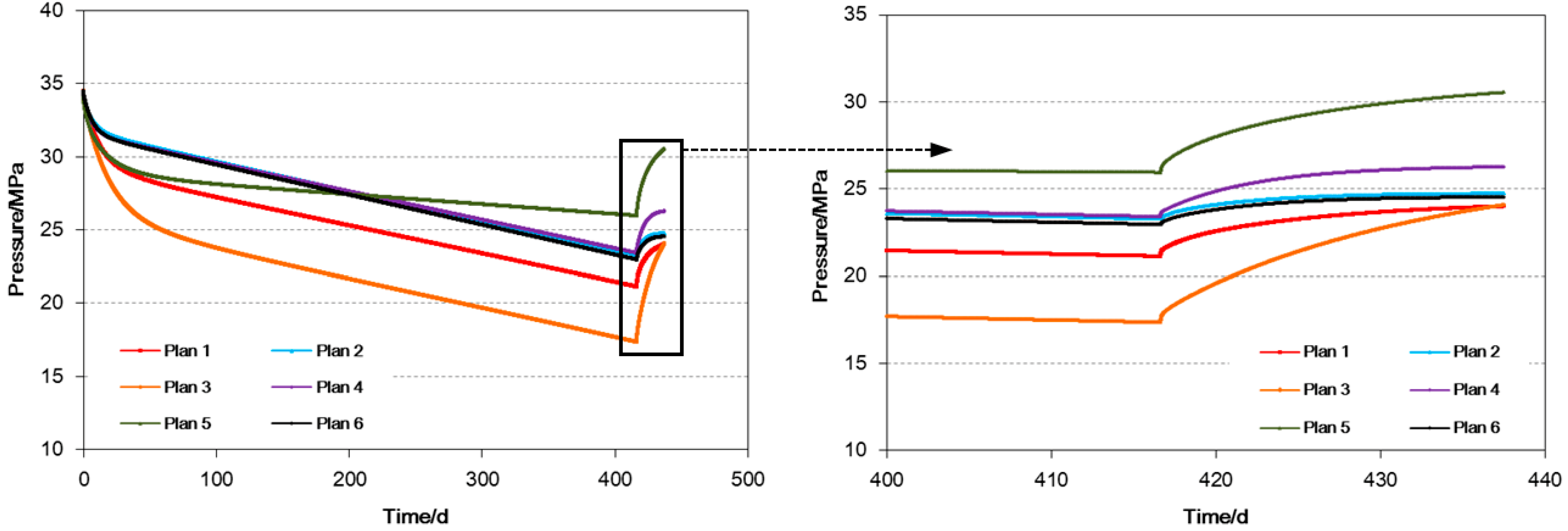
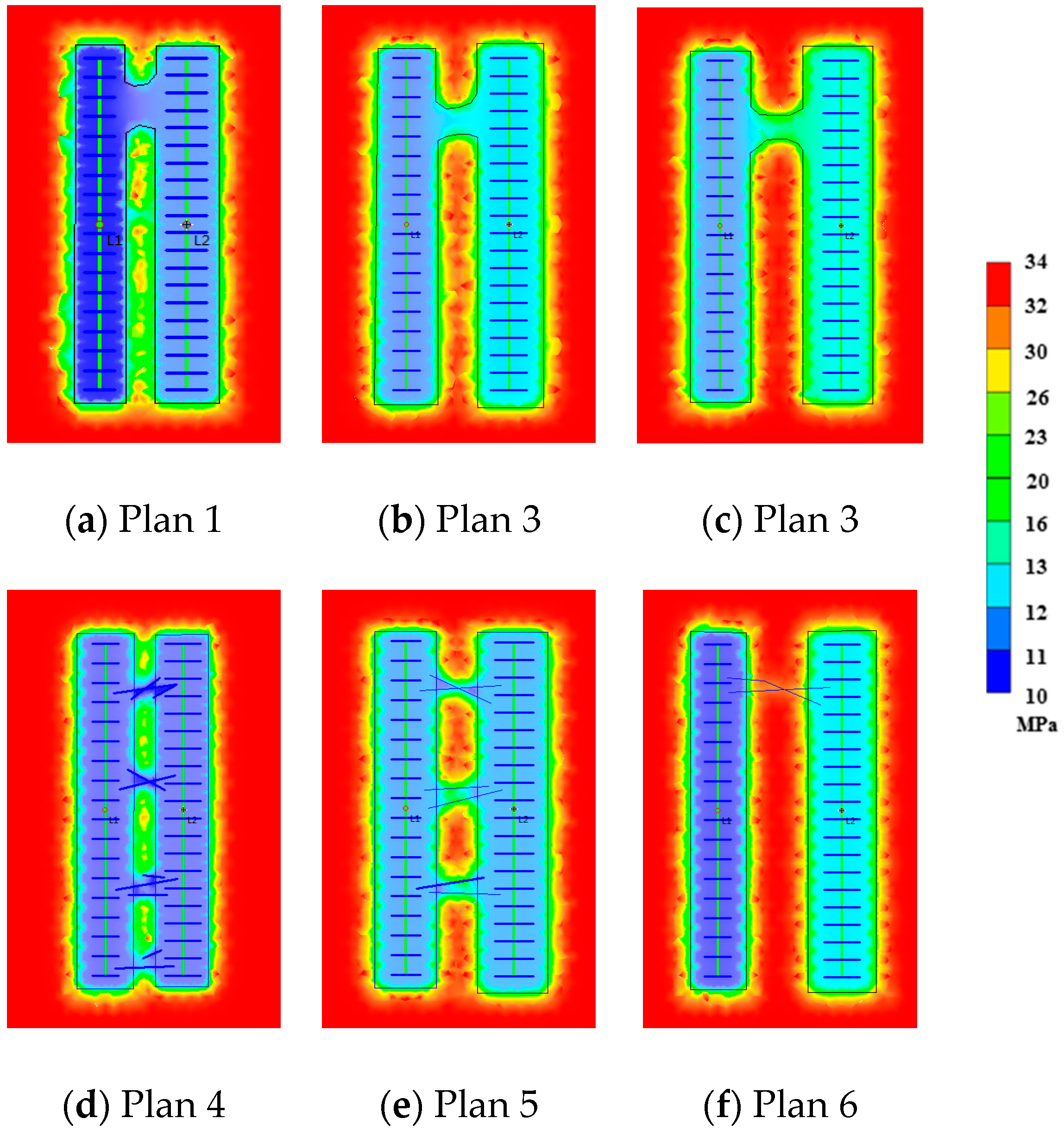
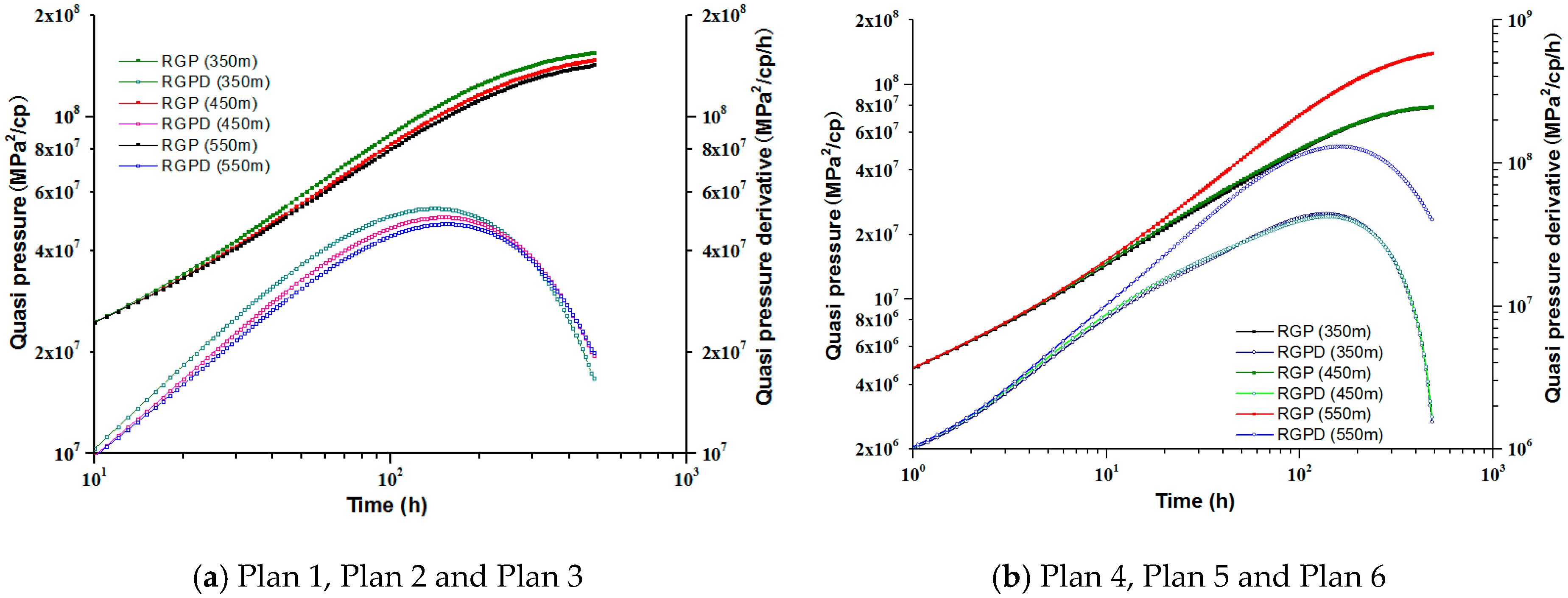
The different connectivity modes and fracturing effects have considerable influence on the seepage characteristics under the disturbance of adjacent wells. By establishing the mechanism model, the effects of hydraulic fracture connected layers, connectivity modes, and the development degree of micro-fractures in SRV on the transient pressure of the well are discussed. A variety of simulation schemes have been designed based on different inter-well connection modes (IWCMs) and SRV parameters. Table 1 shows the IWCMs and essential physical property of each plan. In each scheme, the investigated well (right L2 well) and its neighboring well (left L1 well) are designed to produce at 6 × 10⁴ m3/d for 15 months, and the pressure field around these two wells is shown in Figure 6; afterward, the L2 well is shut-in for 20 days with pressure recovery, while L1 well maintains at the 6 × 10⁴ m3/d gas rate. The BHP of L2 well in each plan is shown in Figure 7, and the double logarithmic curve of the pseudo pressure and its derivative in the shut-in stage is shown in Figure 8.
By analysis of the pressure fields (Figure 6) and the BHP of L2 (Figure 7), several points are obtained as follows:
- (1)
- In Plan 3, induced micro-fractures are not abundant in SRV, and the pressure drop in the SRV is not balanced during the production process, and the pressure near the HFs around the near-well area is severely reduced. However, the overall pressure drop in the SRV is small, so the BHP of L2 well is the largest in the case of the same amount of accumulated gas output. In the latter period, the shut-in pressure recovers the fastest with the greatest extent, but the pressure after recovery is still the lowest.
- (2)
- In Plan 6, the BHP of L2 well is slower and the amplitude is the slowest, and the BHP of L2 shut-in well recoveries faster and higher in the later period, and after the recovery the BHP reaches the highest. In the early stage, due to the poor hydraulic fracturing effect of L2 well, the pressure drops quickly, but in the later period, the pressure drop is not serious due to the interference from the adjacent well. It also shows that even if there is no connection of HF or SRV between the well pairs, there will be some interference.
- (3)
- Comparing Plan 2 and Plan 5 both with strong inter-well connection, the BHP changes of L2 well are very similar. It shows that due to the good effect of fracturing, the SRV area is rich in induced micro-fractures, and the HFs have strong conductivity. Although L2 well gets the interference from neighboring L1 well, the BHP of L2 drops still slowly. After shut-in, disturbed by the production of the neighboring L1 well, the pressure at the later stage of the well shut-in does not recover but decrease, and the inter-well interference is obvious.
- (4)
- In Plan 1, Plan 3, and Plan 6, the two wells have poor fracturing effect and the pressure drop near the HFs is significantly larger than that of the surrounding SRV in each plan. It shows that the pressure drop in the control range of a single well is not balanced enough and the development result is not ideal.
There are two wells in each plan, and L2 on the right is the investigated well, while L1 on the left is the neighboring well.
Through analyzing the pressure recovery curve of each plan in Figure 8, we get the following understanding. (1) the interference degree comes from neighboring wells in each plan is compared based on the fall magnitude in the later part of the pseudo pressure derivative curve (PPDC): Plan 2 > Plan 6 > Plan 4 > Plan1 > Plan 5 > Plan 3; (2) When HFs or SRV’s induce micro-fractures is in rich, it first experience a brief stratum-fracture bilinear flow (the slope of the pseudo pressure derivative curve is close to 1/4), and then it converts to formation linear flow (the slope of the pseudo pressure derivative curve is close to 1/4), late-stage well interference causes the pressure curve to drop. When induced micro-cracks are not abundant, they mainly experience formation linear flow, and the characteristics of later well interference are not obvious.
In summary, BHP changes are affected by both the fracturing effect of the well and interference from neighboring wells. When the fracturing effect of the well is good, and it is connected with the neighboring well through the SRV, the BHP in the production process can drop slowly to maintain stable production. When the fracturing effect of the wells is poor, and some parts are connected with the adjacent well, the BHP decline violently during the production, which is unfavorable to the stable high production of gas wells. In the future production process, it is necessary to reduce the steady gas production and timely shut well to recover the BHP.
4.4. Effect of Well Space
Reasonable well spacing is a crucial indicator for the design of horizontal well patterns to develop shale gas fields. If the well spacing is too small, a severe well interference and a decrease in productivity will appear. Large well spacing will lead to a low recovery of the whole shale gas field, and the remaining reserves will be difficult to exploit in the later period. Therefore, interference degree of different well spacing and different IWMDs should be studied necessarily. We design six plans with different IWMDs and well spacing in the mechanism models, whose basic parameters of each plan are shown in Table 2. In each plan, L2 well and its neighboring well (L1 well) are set to produce at 6 × 10⁴ m3/d for 15 months. The pressure field is shown in Figure 9; after that, the well shut-in and BHP recovers for 20 days. At this time, the neighboring well still maintains 6 × 10⁴ m3/d gas output. The BHP of L2 well in each plan is shown in Figure 10. The double logarithmic curve of the pseudo pressure and its derivative at the shut-in stage is shown in Figure 11.
Through analyzing the BHP and pressure fields of each plan in Figure 9 and Figure 10, we get the following understanding:
- (1)
- From the simulation results of the Plan 1 and Plan 4, when the well spacing is small, the pressure drop in the SRV is severe, and the BHP drop of L2 well is relatively large in the production process, and the shut-in pressure recovery ability is relatively weak, as shown in Figure 9a,d, and Figure 10.
- (2)
- From the simulation results of Plans 3 and 6, the pressure decreasing speed in the SRV is not serious when the well spacing is large, and the BHP of L2 wells is smaller in the production process, and the pressure recovery ability is stronger during well shut-in, as shown in Figure 9c,f and Figure 10.
- (3)
- Compared with the HF connection mode, when the inter-well SRVs connected, the pressure drop of L2 well is slow under the same well spacing in the production process, and the pressure recovery after shut-in is obvious, which indicates that the reservoir still maintains strong energy.
Through analyzing the pressure recovery curve of each plan in Figure 11, we obtain some views as follows:
- (1)
- Under close well spacing and multiple HFs connection modes, the interference comes from neighboring wells is more serious, so this kind of multiple HFs connection should be avoided by controlling hydraulic fracturing;
- (2)
- Under the condition of SRV connection mode, the effect of different well spacing is not obvious, and the well interference is also obvious;
- (3)
- For these mechanism models, the well spacing should be controlled above 450 m. For the development of real shale gas fields, the well spacing can be optimized based on the reservoir physical property and the design scale of fracturing, to obtain higher single well productivity and gas field recovery ratio.
4.5. Effect of Well Pattern and Multiple Neighboring Wells
Shale gas field development generally adopts a large-scale horizontal well pattern, and there may be multiple adjacent wells around a well. Based on the mechanism model, the simulation plans for different number of wells and different arrangements are designed, and the designed parameters are shown in Table 3. The wells of each scheme are designed to produce at 6 × 10⁴ m3/d for 15 months, and the pressure fields are shown in Figure 12. Afterwards, the BHP of the shut-in L2 well recovers for 20 days. At this time, the neighboring wells all maintain at 6 × 10⁴ m3/d gas output. The BHP of L2 well in each plan is shown in Figure 13. The double logarithm curve of the pseudo pressure and its derivative during the shut-in stage is shown in Figure 14.
By analysis of the pressure fields (Figure 12) and the BHP of L2 (Figure 13), several points are obtained as follows. (1) When well spacing keeps at 350m, increasing number of neighboring wells do not lead to serious pressure drop in the SRV of L2 well. Besides, the pressure drop is not apparent in the outside matrix, but the pressure drop is significant in SRV with HFs connected. (2) Corresponding and connecting with the direct neighboring wells’ horizontal segment is the key to generate obvious interference. If the corresponding inter-well horizontal segment is more extended, the interference is more severe (compared Plan 1 with Plan 2). On this basis, the more interconnected wells put into production in the well pattern, the more severe interference is, and even if only the ends of the horizontal well (toe or root) are connected, interference still occurs. (3) Under the condition of the same number of connected neighboring wells, no matter what the well spacing and IWMDs are, the BHP curve is nearly overlapped. It indicates that the number of neighboring wells is crucial to the well interference degree, and the number of HFs connected is relatively secondly. (4) The more severe interference the neighboring wells lead, the more severe the performance is, as well as the fact that BHP in the well is declining faster in the production phase. Even though the neighboring well is not directly adjacent to the well, it is indirectly adjacent to one well after it has been sequestered by one well and still interferes with the well (compared Plan 2 with Plan 3).
Through analyzing the pressure recovery curve of each plan in Figure 14, we obtain some views as follows. (1) Parallel arrangements produce more severe well interference than head-to-head arrangements under a same number of wells. (2) The pseudo pressure derivative curve of each plan shows the characteristics of linear flow, quasi-radial flow segment and pressure drop disturbed by adjacent wells. (3) When the parameters such as HF properties and gas production keep constant, the linear flow in the early stage of each plan is the same, and the difference mainly lies in the late interference stage.
5. Field Application
A2 is a well group (five wells) in the lower gas zone of the Longmaxi section of the Lower Silurian in the Jiaoshiba shale gas field. Log interpretation explains an average porosity of 3.94%, an average permeability of 0.02 mD to 0.06 mD, and an average gas content of 3.47 m3/t to 3.85 m3/t. The gas composition is dominated by methane (98.4%) and contains a small amount of ethane, carbon dioxide and nitrogen; the initial formation pressure is 32.3 MPa and the initial temperature is 94.7 °C. During the drilling process, there is no leakage of drilling fluid in the horizontal well section. Each well in the well group put into operation from April 2014. As of March 2018, the cumulative gas production of Well A2-1 was 6272.28 × 104 m3/d, and the average daily gas production was 6.41 × 10⁴ m3/d, and the casing pressure dropped from initial 29.4 MPa to 10.7 MPa. The cumulative gas production of A2-2 well is 9633.57 × 104 m3/d, and the average daily gas production is 8.17 × 10⁴ m3/d, and the casing pressure reduced from 29.3 MPa to 8.9 MPa. Accumulated gas production in Well A2-3 is 6143.43 × 104 m3/d, and average daily gas production is 5.21 × 10⁴ m3/d, and casing pressure reduced from 31.8 MPa to 13.3 MPa. Accumulated gas production in Well A2-4 is 8515.55 × 104 m3/d, average daily gas production is 8.95 × 10⁴ m3/d, and casing pressure is reduced from 30MPa to 13.4 MPa. The cumulative gas production of Well A2-5 is 5471.0 × 104 m3/d, the average daily gas production is 7.00 × 10⁴ m3/d, and the casing pressure is reduced from 31.4 MPa to 16.4 MPa.
By performing pressure recovery tests on well A2-1 in the center of the well group, inversion of reservoir and fracture property parameters, and analysis of interference from neighboring wells to production. According to the basic parameters of the reservoir, the position relationship of each well, the scale of fracturing construction in each section of the horizontal well, and the tracer test results, a numerical well test model was established to analyze the pressure recovery test data. The simulation results of the simulated pressure field and the pseudo-logarithmic double logarithmic curve are shown in Figure 15. From the simulated pressure field of the numerical well test in Figure 15a, the wells A2-4 and A2-5 arranged opposite to the A2-1 well have weak interference to them. The A2-2 wells arranged in parallel with it and connected to the SRV have strong interference to them, and the A2-3 wells with relatively long distances have weak interference to them. From the plot of the double logarithm curve of the pseudo-pressure in Figure 15b, the lower part of the curve falls, but the amplitude is not large; it shows that there are not many adjacent wells that interfere with it, and there is no multi-segment fracture crack connectivity.
In order to further verify the interference of 4 neighboring wells to the central well A2-1, the gas production and pressure of the adjacent wells during the pressure recovery of this well were compared (Figure 16). During the recovery of pressure in this well, well A2-2 was normally produced but the pressure decreased slowly or even recovered. The rate of decline of the other three wells did not change substantially during this period. It is confirmed that well A2-2 has a significant influence on well A2-1, which is in agreement with the conclusion of numerical well test analysis. In short, the interference between the two wells is relatively small (A2-1 and A2-4, A2-5), but the interference is smaller when the well spacing is larger (A2-1 and A2-3). Although A2-1 and A2-2 wells interfered with the SRV mode, they did not cause serious pressure drop.
6. Conclusions
In recent years, with the continuous expansion of the shale gas wells pattern’s scale and reduction of well spacing, the problem of well interference has become increasingly serious. On the one hand, the shale gas well interference leads BHP drops rapidly, which is harmful to gas production; on the other hand, under the condition of a relatively balanced fracturing scale, it shows that the IWCM is good and can effectively control the resources within the reservoir around the well. In fact, the scale of most fracturing sections of most shale gas wells is not balanced. Interferences are mainly appeared between the wells with good fracturing and close well spacing.
To study transient pressure behaviors of shale gas MFHW under well interference, we establish a multi-region coupled flow model based on the pore fracture structures and flow mechanisms of the different region. Then, PEBI grids and finite volume method are used for the numerical solution. Utilizing the measured shut-in pressure recovery test data of shale gas wells, we explain the property parameters of the reservoir and HFs. Moreover, BHP data monitored in the later stage is fitted to verify the accuracy of the model. Based on the shale gas seepage model, the pressure field and BHP are analyzed under the disturbance of adjacent wells.
The transient pressure behaviors of shale gas wells are affected by fracturing effect, production rules, and well interference. The interference can be observed from the later decline phase of the PPDC during well shut-in. Different IWCM, well spacing, number of neighboring wells, and well pattern arrangement lead different PPDC drops extent in the later phase. A sharp BHP drop can be caused by the direct inter-well connection of HFs, which also has a severe influence on the pressure recovery of the shut-in wells. Sometimes, well interference still exists even without direct HF connection, which reflects the SRV connected with satisfied fracturing effect. It is conducive to higher recovery. Generally, we recommend that it is necessary to optimize the well spacing and the fracturing scale according to the stimulated performance. Especially, the fracturing scale should be controlled for the segments close to the neighboring well; and if serious disturbances have already occurred, it is necessary to timely control the gas production of this well pair, and timely conduct interference test to quantify the degree of interference.
Author Contributions
Conceptualization, D.G. and Y.L.; methodology, D.G.; validation, G.H.; formal analysis, D.G.; investigation, D.G.; resources, D.G.; data curation, D.G.; writing—original draft preparation, D.G.; writing—review and editing, D.W.; visualization, D.G.; supervision, Y.L.; project administration, Y.L.; funding acquisition, D.G.
Funding
This research was funded by Southwest Petroleum University of Open Fund of State Key Laboratory of Oil and Gas Reservoir Geology and Exploitation, grant number PLN201711 and National Natural Science Foundation of China, grant number 11702300 and PetroChina Innovation Fundation, grant number 2017D-5007-0208.
Acknowledgments
The study was supported by Supported By Open Fund (PLN201711) of State Key Laboratory of Oil and Gas Reservoir Geology and Exploitation (Southwest Petroleum University), National Natural Science Foundation of China (11702300), PetroChina Innovation Fundation (2017D-5007-0208) and the Key Laboratory of Fluid-Solid Coupling System Mechanics, Chinese Academy of Sciences.
Conflicts of Interest
The authors declare no conflict of interest.
Nomenclature
mF is the gas pseudo pressure of HF, MPa2/(mPa·s); mS,m and mS,f are the gas pseudo pressure of the SRV matrix system and fracture system respectively, MPa2/(mPa·s); F and S are the marks of HF and SRV respectively, dimensionless; m and f are the marks of SRV matrix system and fracture system respectively, dimensionless; qiw,F is the fluid exchange volume between the HF and wellbore, m3/d; φ is porosity, dimensionless; kF is the permeability of HF with finite conductivity, mD; μg is gas viscosity, mPa·s; cg is gas compressibility factor, MPa−1; t is time, d; α is exchange flow coefficient, (m3·mPa·s)/MPa2; VS,L is Langmuir gas volume, m3/kg; Vstd is gas molar volume at standard temperature and pressure conditions, m3/kmol; mS,L is Langmuir gas pressure, MPa2/(mPa·s); MS,g is gas molar weight, kg/kmol; Kn is knudsen number, dimensionless; β is tenuity factor, dimensionless; b is average fracture aperture, m; c is average fracture interval, m.
References
- Ma, X.; Xie, J. The progress and prospects of shale gas exploration and development in southern Sichuan Basin, SW China. Pet. Explor. Dev. 2018, 45, 161–169. [Google Scholar] [CrossRef]
- Zou, C.; Yang, Z.; He, D.; Wei, Y.; Li, J.; Jia, A.; Chen, J.; Zhao, Q.; Li, Y.; Li, J.; et al. Theory, technology and prospects of conventional and unconventional natural gas. Pet. Explor. Dev. 2018, 45, 1–13. [Google Scholar] [CrossRef]
- Wang, Z. Breakthrough of Fuling shale gas exploration and development and its inspiration. Oil Gas Geol. 2015, 36, 1–6. [Google Scholar]
- Ilkay, U.; Basak, K.; Hossein, K. Multiphase rate-transient analysis in unconventional reservoirs: Theory and application. SPE Reserv. Eval. Eng. 2016, 19, 1–14. [Google Scholar]
- Soeder, D.J. The successful development of gas and oil resources from shales in North America. J. Pet. Sci. Eng. 2018, 163, 399–420. [Google Scholar] [CrossRef]
- Ajani, A.A.; Kelkar, M.G. Interference study in shale plays. SPE 151045. In Proceedings of the SPE Hydraulic Fracturing Technology Conference, Woodlands, TX, USA, 6–8 February 2012. [Google Scholar]
- Manchanda, R.; Sharma, M.M.; Holzhauser, S. Time-dependent fracture-interference effects in pad wells. SPE Prod. Oper. 2014, 29, 1–14. [Google Scholar] [CrossRef]
- Sardinha, C.M.; Lehmann, J.; Pyecroft, J.F.; Petr, C.; Merkle, S. Determining interwell connectivity and reservoir complexity through frac pressure hits and production interference analysis. SPE-171628-MS. In Proceedings of the SPE/CSUR Unconventional Resources Conference, Calgary, AB, Canada, 30 September–2 October 2014. [Google Scholar]
- Cheng, L.; Jia, P.; Rui, Z.; Huang, S.; Xue, Y. Transient responses of multifractured systems with discrete secondary fractures in unconventional reservoirs. J. Nat. Gas Sci. Eng. 2017, 41, 49–62. [Google Scholar] [CrossRef]
- Zhu, W.; Qi, Q.; Ma, Q.; Deng, J.; Yue, M.; Liu, Y. Unstable seepage modeling and pressure propagation of shale gas reservoirs. Pet. Explor. Dev. 2016, 43, 261–267. [Google Scholar] [CrossRef]
- Mezghani, M.; Roggero, F. Combining gradual deformation and upscaling techniques for direct conditioning of fine scale reservoir models to interference test data. SPE J. 2004, 9, 79–87. [Google Scholar] [CrossRef]
- Yaich, E.; Souza, O.C.D.D.; Foster, R.A.; Abou-Sayed, I.S. A methodology to quantify the impact of well interference and optimize well spacing in the marcellus shale. SPE-171578-MS. In Proceedings of the SPE/CSUR Unconventional Resources Conference, Calgary, AB, Canada, 30 September–2 October 2014. [Google Scholar]
- Marongiu-Porcu, M.; Lee, D.; Shan, D.; Morales, A. Advanced modeling of interwell-fracturing interference: An eagle ford shale-oil study. SPE J. 2015, 21, 1567–1582. [Google Scholar] [CrossRef]
- Pang, W.; Ehlig-Economides, C.A.; Du, J.; He, Y.; Zhang, T. Effect of well interference on shale gas well SRV interpretation. SPE 176910. In Proceedings of the SPE Asia Pacific Unconventional Resources Conference and Exhibition, Brisbane, Australia, 9–11 November 2015. [Google Scholar]
- Bello, R.O.; Wattenbarger, R.A. Multi-stage hydraulically fractured shale gas rate transient analysis. SPE 126754. In Proceedings of the North Africa Technical Conference and Exhibition, Cairo, Egypt, 14–17 February 2010. [Google Scholar]
- Ozkan, E.; Brown, M.L.; Raghavan, R.; Kazemi, H. Comparison of fractured horizontal well performance in tight sand and shale reservoirs. SPE Reserv. Eval. Eng. 2011, 14, 248–259. [Google Scholar] [CrossRef]
- Al-Rbeawi, S. Analysis of pressure behaviors and flow regimes of naturally and hydraulically fractured unconventional gas reservoirs using multi-linear flow regimes approach. J. Nat. Gas Sci. Eng. 2017, 45, 637–658. [Google Scholar] [CrossRef]
- Stalgorova, E.; Mattar, L. Practical analytical model simulate production of horizontal wells with Branch Fractures. SPE 162515. In Proceedings of the SPE Canadian Unconventional Resources Conference, Calgary, AB, Canada, 30 October–1 November 2012. [Google Scholar]
- Zhang, L.; Gao, J.; Hu, S.; Guo, J.; Liu, Q. Five-region flow model for MFHWs in dual porous shale gas reservoirs. J. Nat. Gas Sci. Eng. 2016, 33, 1316–1323. [Google Scholar] [CrossRef]
- Zeng, J.; Wang, X.; Guo, J.; Zeng, F. Composite linear flow model for multi-fractured horizontal wells in heterogeneous shale reservoir. J. Nat. Gas Sci. Eng. 2017, 38, 527–548. [Google Scholar] [CrossRef]
- Wang, J.; Jia, A.; Wei, Y.; Qi, Y. Approximate semi-analytical modeling of transient behavior of horizontal well intercepted by multiple pressure-dependent conductivity fractures in pressure-sensitive reservoir. J. Pet. Sci. Eng. 2017, 153, 157–177. [Google Scholar] [CrossRef]
- Kim, T.H.; Lee, J.H.; Lee, K.S. Integrated reservoir flow and geomechanical model to generate type curves for pressure transient responses of a hydraulically-fractured well in shale gas reservoirs. J. Pet. Sci. Eng. 2016, 146, 457–472. [Google Scholar] [CrossRef]
- Xiong, X.; Devegowda, D.; Michel Villazon, G.G.; Sigal, R.F.; Civan, F. A fully-coupled free and adsorptive phase transport model for shale gas reservoirs including non-darcy flow effects. SPE 159758. In Proceedings of the SPE Annual Technical Conference and Exhibition, San Antonio, TX, USA, 8–10 October 2012. [Google Scholar]
- Xu, B.; Haghighi, M.; Li, X.; Cooke, D.; Zhang, L. Development of new type curves for production analysis in naturally fractured shale gas/tight gas reservoirs. J. Pet. Sci. Eng. 2013, 105, 107–115. [Google Scholar] [CrossRef]
- Gu, A.; Ding, D.; Gao, Z.; Zhang, A.; Tian, L.; Wu, T. Pressure transient analysis of multiple fractured horizontal wells in naturally fractured unconventional reservoirs based on fractal theory and fractional calculus. Petroleum 2017, 3, 326–339. [Google Scholar] [CrossRef]
- Fan, D.; Yao, J.; Sun, H.; Zeng, H. Numerical simulation of multi-fractured horizontal well in shale gas reservoir considering multiple gas transport mechanisms. Acta Mech. Sin. 2015, 47, 906–915. [Google Scholar]
- Bonyadi, M.; Rahimpour, M.R.; Esmaeilzadeh, F. A new fast technique for calculation of gas condensate well productivity by using pseudopressure method. J. Nat. Gas Sci. Eng. 2012, 4, 35–43. [Google Scholar] [CrossRef]
- Hull, R.; Bello, H.; Richmond, P.L.; Suliman, B.; Portis, D.; Richmond, P. Variable stimulated reservoir volume (SRV) simulation: Eagle ford shale case study. URTEC 1582061. In Proceedings of the Unconventional Resources Technology Conference, Denver, CO, USA, 12–14 August 2013. [Google Scholar]
- Civan, F.; Rai, S.C.; Sondergeld, H.C. Shale-gas permeability and diffusivity inferred by improved formulation of relevant retention and transport mechanisms. Transp. Porous Media 2010, 86, 925–944. [Google Scholar] [CrossRef]
- Civan, F. Effective correlation of apparent gas permeability in tight porous media. Transp. Porous Media 2010, 82, 375–384. [Google Scholar] [CrossRef]
- Ye, Z.; Chen, D.; Pan, Z. A unified method to evaluate shale gas flow behaviours in different flow regions. J. Nat. Gas Sci. Eng. 2015, 26, 205–215. [Google Scholar] [CrossRef]
- Singh, H.; Javadpour, F.; Ettehadtavakkol, A.; Darabi, H. Nonempirical apparent permeability of shale. SPE Reserv. Eval. Eng. 2014, 17, 1–15. [Google Scholar] [CrossRef]
- Moyner, O.; Lie, K.A. The multiscale finite volume method on unstructured grids. SPE 163649. In Proceedings of the SPE Reservoir Simulation Symposium, Woodlands, TX, USA, 18–20 February 2013. [Google Scholar]
- Dejam, M. Advective-diffusive-reactive solute transport due to non-Newtonian fluid flows in a fracture surrounded by a tight porous medium. Int. J. Heat Mass Transf. 2019, 128, 1307–1321. [Google Scholar] [CrossRef]
- Dejam, M.; Hassanzadeh, H.; Chen, Z. Pre-darcy flow in tight and shale formations. In Proceedings of the 70th Annual Meeting of the APS (American Physical Society) Division of Fluid Dynamics, Denver, CO, USA, 19–21 November 2017. [Google Scholar]
Figure 1.
Multi-region coupled shale reservoir physical model (Well-A and well-B are two multi-stage fracturing horizontal wells (MFHWs), the hydraulic fractures connected with the SRV and the SRVs are dual medium.).
Figure 1.
Multi-region coupled shale reservoir physical model (Well-A and well-B are two multi-stage fracturing horizontal wells (MFHWs), the hydraulic fractures connected with the SRV and the SRVs are dual medium.).

Figure 2.
Perpendicular bisection (PEBI) meshing grids of HFs and matrix.

Figure 3.
Double logarithmic curve fitting results for pressure recovery in well A1-1.

Figure 4.
A1-1 bottomhole pressure (BHP) fitting results (A1-3 was a new neighboring well produced at June 2017).
Figure 4.
A1-1 bottomhole pressure (BHP) fitting results (A1-3 was a new neighboring well produced at June 2017).

Figure 5.
Mechanism model of two adjacent shale gas wells.

Figure 6.
Pressure distribution after 15 months of simulated production of different plan.

Figure 7.
BHP changes during production and shut-in of L2 well.

Figure 8.
Double logarithmic curve of L2 well recovery pseudo pressure of each plan.

Figure 9.
Pressure fields of six plans after producing 15 months under different well spacing.

Figure 10.
BHP of L2 well after producing 15 months under different well spacing.

Figure 11.
Double logarithmic curves of L2 build-up pressure under different well spacing.

Figure 12.
Pressure field under different well pattern and multiple neighboring wells in six designed plans.
Figure 12.
Pressure field under different well pattern and multiple neighboring wells in six designed plans.

Figure 13.
BHP of L2 well with different well pattern and multiple neighboring wells.

Figure 14.
Double logarithmic curve of pressure recovery of shut-in wells under different well pattern and multiple neighboring wells.
Figure 14.
Double logarithmic curve of pressure recovery of shut-in wells under different well pattern and multiple neighboring wells.

Figure 15.
Numerical well of the simulation results of the simulated pressure field and the pseudo-logarithmic double logarithmic curve.
Figure 15.
Numerical well of the simulation results of the simulated pressure field and the pseudo-logarithmic double logarithmic curve.

Figure 16.
Gas production and pressure of A2 well group.


Table 1.
Inter-well communication modes (IWCMs) and essential physical properties of each plan.
| Plan | IWCMs | HF Conductivity/mD·m | HF Half-Length/m | SRV Permeability/mD | Matrix Permeability/mD |
|---|---|---|---|---|---|
| Plan 1 | One HF connected | 20 | 60 | 0.3 | 0.0003 |
| Plan 2 | Four HFs connected | 20 | 60 | 0.6 | 0.0003 |
| Plan 3 | One SRV segment connected with induced micro-fractures | 20 | 60 | 0.15 | 0.0003 |
| Plan 4 | One SRV segment connected with abundant induced micro-fractures | 20 | 60 | 0.6 | 0.0003 |
| Plan 5 | Two SRV segments and HF connected | 20 | 60 | 0.6 | 0.0003 |
| Plan 6 | No SRV or HF connected | 20 | 60 | 0.15 | 0.0003 |
Table 2.
IWMDs and basic physical properties of six plans.
| Plan | IWCMs | HF Conductivity/mD·m | HF Half-Length/m | SRV Permeability/mD | Matrix Permeability/mD |
|---|---|---|---|---|---|
| Plan 1 | Well spacing 350 m with SRV connected | 20 | 60 | 0.06 | 0.0003 |
| Plan 2 | Well spacing 450 m with SRV connected | 20 | 60 | 0.06 | 0.0003 |
| Plan 3 | Well spacing 550 m with SRV connected | 20 | 60 | 0.06 | 0.0003 |
| Plan 4 | Well spacing 350 m with four HFs connected | 200 | 60 | 0.06 | 0.0003 |
| Plan 5 | Well spacing 450 m with two HFs connected | 200 | 60 | 0.06 | 0.0003 |
| Plan 6 | Well spacing 550 m with one HFs connected | 200 | 60 | 0.06 | 0.0003 |
Table 3.
IWMDs and basic physical properties of six plans.
| Plan | IWCMs | HF Conductivity/mD·m | HF Half-Length/m | SRV Permeability/mD | Matrix Permeability/mD |
|---|---|---|---|---|---|
| Plan 1 | Three wells: L2 well and two adjacent wells (L1 and L3) with seven HFs connected. | 100 | 60 | 0.03 | 0.0003 |
| Plan 2 | Three wells: L2 well is staggered with two adjacent wells (L1 and L3), and four HFs connected in the corresponding well segments. | 100 | 60 | 0.03 | 0.0003 |
| Plan 3 | Four wells: L2 well and two adjacent wells (L1 and L3) connected through five HFs, and L1 well connects with L4 well by two HFs. | 100 | 60 | 0.03 | 0.0003 |
| Plan 4 | Four wells: L2 well is parallel with two adjacent wells (L1 and L3), and head-to-head with L4 well. There are eight HFs connected. | 100 | 60 | 0.03 | 0.0003 |
| Plan 5 | Five wells: L2 well, and two neighboring wells (L3 and L4) on the left side and two neighboring wells (L1 and L5) on the right side, and total nine HFs connected. | 100 | 60 | 0.03 | 0.0003 |
| Plan 6 | Six wells: L2 well is parallel with two neighboring wells (L1 and L3), and head-to-head with three wells (L4, L5 and L6) | 100 | 60 | 0.03 | 0.0003 |
© 2019 by the authors. Licensee MDPI, Basel, Switzerland. This article is an open access article distributed under the terms and conditions of the Creative Commons Attribution (CC BY) license (http://creativecommons.org/licenses/by/4.0/).
Share and Cite
MDPI and ACS Style
Gao, D.; Liu, Y.; Wang, D.; Han, G. Numerical Analysis of Transient Pressure Behaviors with Shale Gas MFHWs Interference. Energies 2019, 12, 262. https://doi.org/10.3390/en12020262
AMA Style
Gao D, Liu Y, Wang D, Han G. Numerical Analysis of Transient Pressure Behaviors with Shale Gas MFHWs Interference. Energies. 2019; 12(2):262. https://doi.org/10.3390/en12020262
Chicago/Turabian StyleGao, Dapeng, Yuewu Liu, Daigang Wang, and Guofeng Han. 2019. "Numerical Analysis of Transient Pressure Behaviors with Shale Gas MFHWs Interference" Energies 12, no. 2: 262. https://doi.org/10.3390/en12020262
Note that from the first issue of 2016, this journal uses article numbers instead of page numbers. See further details here.