Pipeline Leak Detection and Location Based on Model-Free Isolation of Abnormal Acoustic Signals

Abstract

Pipeline leaks will lead to energy waste, environmental pollution and a threat to human safety. This paper proposes a pipeline leak detection and location method based on the model-free isolation of abnormal (leak and operation) signals. An acoustic signal is first decomposed into “sub-signals” according to its zero-crossing points. Then, based on the definition of signal-to-noise ratio (SNR), the function between the SNR of sub-signal and the number of abnormal sub-signals is established, following which the position of each abnormal sub-signal in the acoustic signal is obtained by tracing its index. Based on this and the cross-correlation analysis, the operation sub-signals can be filtered, which is helpful for the precise leak location. The experimental results demonstrate the computational efficiency and lower false/missing alarm rate of the proposed method that provides an innovative solution for pipeline leak detection.

1. Introduction

Pipelines are critical infrastructure to a country’s economy for oil transportation. However, owing pipeline aging, corrosion and destruction of the third parties, pipeline leak accidents often occur [1,2,3,4,5]. For the transport of certain hazardous substances (such as natural gas and hydrogen), pipeline leaks frequently result in serious safety accidents [6,7]. Therefore, pipeline leak detection is necessary. Accordingly, domestic and foreign scholars have conducted considerable research in this area [8,9,10,11,12]. Generally, these pipeline leak detection methods using a classifier are defined as model-based, while others are model-free-based methods.

Many studies have focused on model-based pipeline leak detection methods. In these methods, leak diagnosis models are established by mapping the relationship between feature space and fault space. (1) Feature extraction. From the time-domain perspective, researchers often utilize features of mean, peak, root-mean-square, shape factor, kurtosis, absolute amplitude and relative amplitude [13,14]. From the frequency-domain perspective, according to the relationship between the cepstrum peak and the signal energy, the cepstrum peak is employed as a feature to identify leak signals [4]. From the time-frequency-domain perspective, time-frequency analysis methods (such as wavelet packet, empirical mode decomposition, local mean decomposition, etc.) are often utilized to process signals, and their coefficients combined with root-mean-square or entropy are as features [6,15,16]. (2) Diagnosis model. Some classification methods, such as the support vector domain description (SVDD) [17,18], support vector machine (SVM) [19,20] and Bayesian classifier [21], have been successfully applied to pipeline leak detection [22,23,24,25].

However, since model-based methods take the whole signal as the detection object, they can only judge whether it is abnormal and cannot give the local information (number, amplitude, position) of the abnormality in the signal. In practical applications, it is critical to obtain the local information of anomalies in an acoustic signal to solve false/missing alarms caused by the operation and leak mixing in an acoustic signal. Additionally, many model-based methods rely on leak samples. However, actual leak samples are not available from a real pipeline transportation process. Even if they are usually replaced by artificially simulated leaks, the number of samples is still limited and not able to cover all the leak situations. And for these pipelines of the transportation of certain dangerous substances such as natural gas, hydrogen and liquid chlorine, the artificially simulated leaks are usually generated with water or air as the replacement [16,26,27], which will affect the extracted features. To address this problem, Martini et al. [28] combined the autocorrelation function with the kurtosis to detect water leaks. And experimental results show the validity of this method but more verification of field water pipelines is needed. Wang et al. [14] utilized time domain statistical features of normal samples to establish a diagnosis model based on SVDD. The test results demonstrated that this method offered a certain extent of universality. However, this method was with an estimation of the misclassification rate, which may cause false and missing alarms in the long term continuous operation.

Therefore, this paper proposes a pipeline leak detection and location method based on the model-free isolation of abnormal acoustic signals. For acoustic sensor based leak detection, the operation signals generated by station operations (such as the pressure regulating) will be identified as abnormal signals as well in this paper. According to the bipolar characteristic of the acoustic signal, it can be decomposed into sub-signals. In an acoustic signal, the abnormal sub-signal is as the valid signal and the normal sub-signal as the background noise. Based on this, the functional relationship between the SNR of sub-signal and the number of abnormal sub-signals is established. Then, the direct isolation of abnormal signals can be realized. The proposed method reduces the dependency on samples and does not require feature extraction and diagnosis models, which aids in reducing the occurrence of false and missing alarms. Furthermore, the number of abnormal sub-signals and their positions in an acoustic signal can be obtained simultaneously, which helps to improve the location precision.

The composition of this paper is: Section 2 introduces the leak detection system based on the acoustic sensor; Section 3 and Section 4 describe the model-free-based abnormal signal isolation method and the leak precise location method, respectively; Section 5 presents experiments; and Section 6 summarize this paper.

2. Acoustic Sensor-Based Leak Detection System

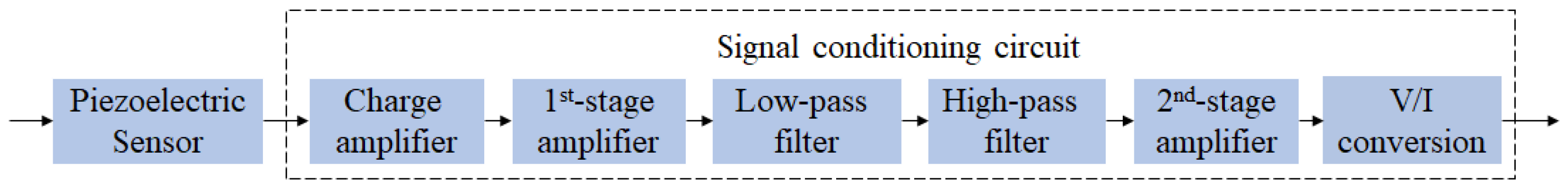
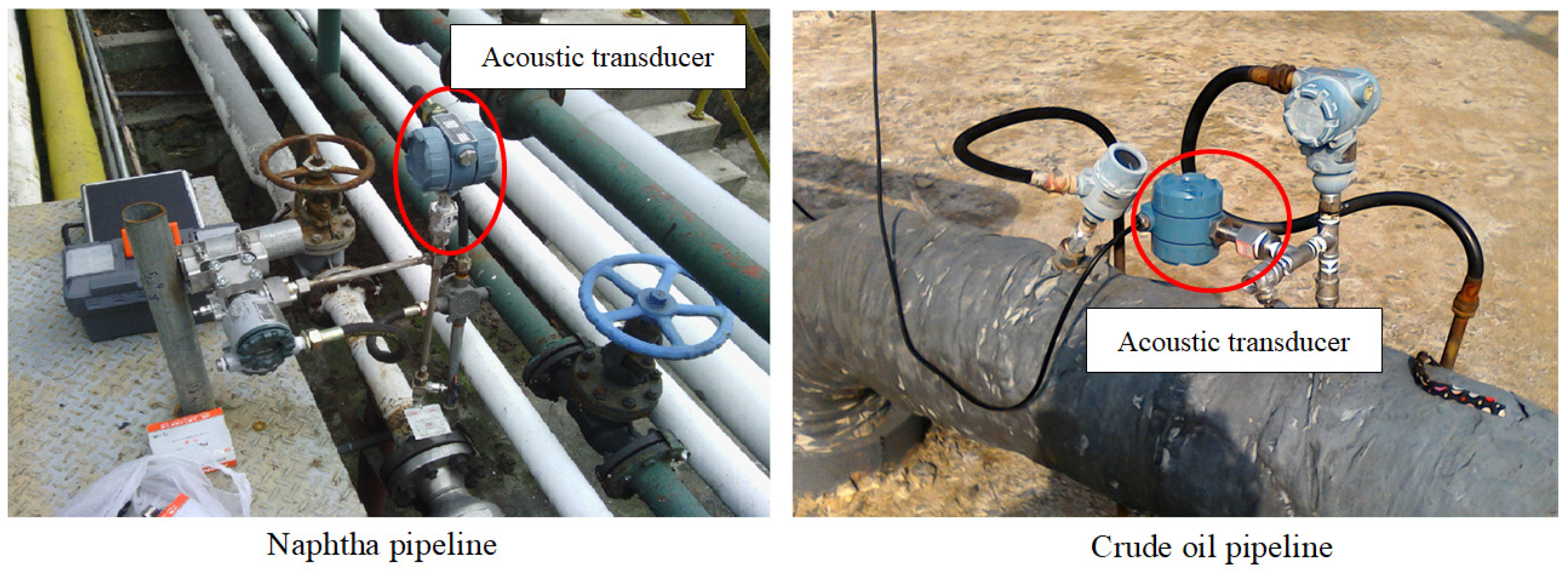
The schematic configuration of the pipeline leak detection system is shown in Figure 1. The acoustic transducer consists of a piezoelectric pressure sensor and signal conditioning circuit. The piezoelectric pressure sensor is used to sense acoustic signals and convert them into charge signals. The circuit mainly includes a charge amplifier, a low- and high-pass filter, two voltage amplifiers and a voltage/current converter, as shown in Figure 2. After charge signals are processed by the circuit, they are remotely transmitted to the remote terminal units in the form of current (4∼20 mA). The synchronous acquisition of upstream and downstream acoustic signals can be achieved by GPS timing. Finally, these digital acoustic signals are sent to the computer center via the Internet for leak detection. Figure 3 shows the field installation of the acoustic transducers on pipelines.

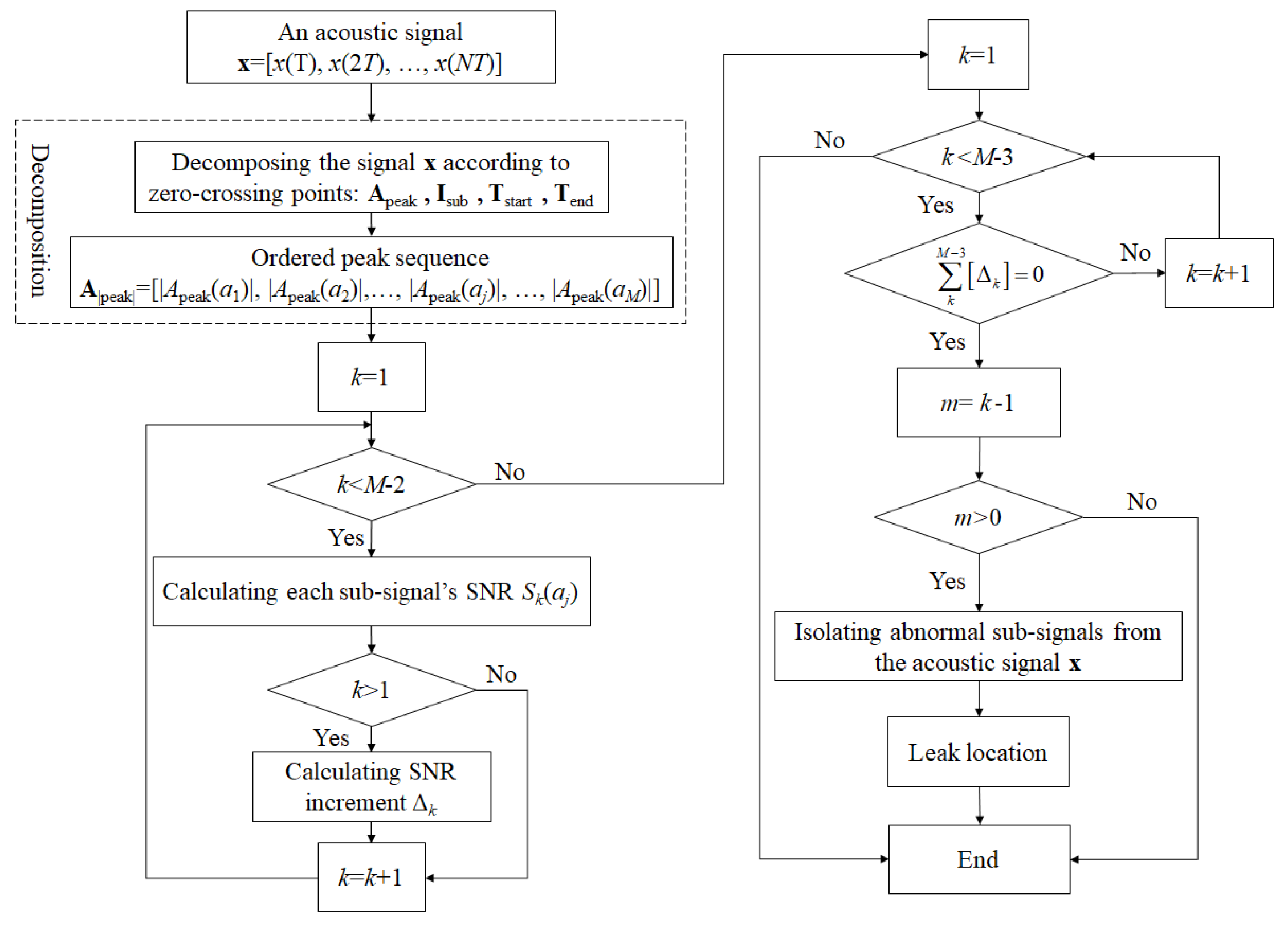
3. Model-Free Isolation Principle of Abnormal Acoustic Signals

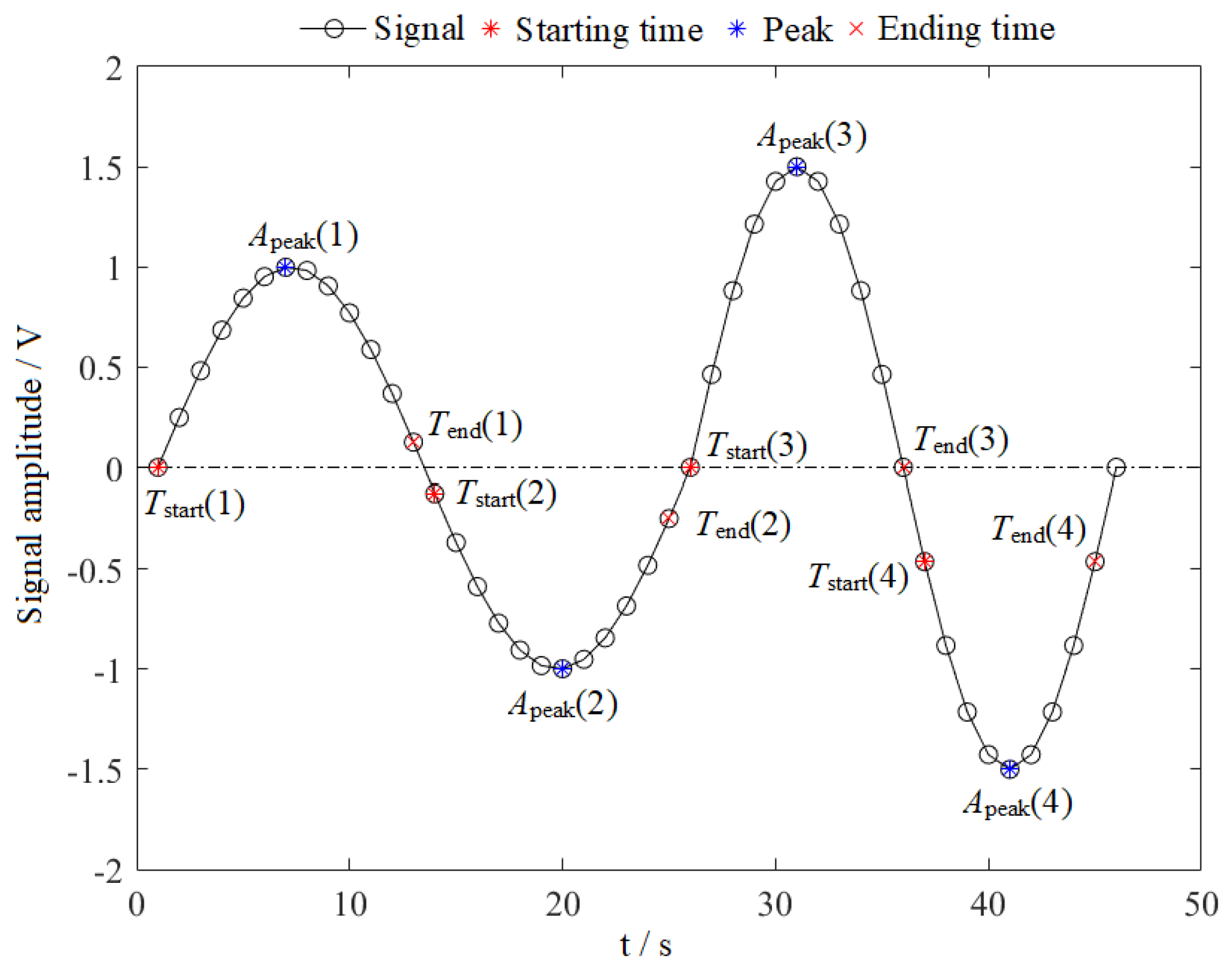
3.1. Decomposition of an Acoustic Signal

The bipolarity of the acoustic signal $\mathbf{x}$ makes it possible to decompose the signal into positive and negative intervals with the zero-crossing points and each interval is regarded as a sub-signal. An acoustic signal is denoted by:

$$\mathbf{x}=\left[x\right(T),x(2T),\dots ,x(NT\left)\right]$$

(1)

where N is the data length of the acoustic signal $\mathbf{x}$, T is the sampling period. Based on the zero-crossing points of $\mathbf{x}$, the acoustic signal can be decomposed into M sub-signals and each sub-signal ${\mathbf{x}}_{\mathrm{sub}}\left(j\right)$ is:

$${\mathbf{x}}_{\mathrm{sub}}\left(j\right)=[x\left(T_{\mathrm{start}}\left(j\right)\right),\dots ,x\left(T_{\mathrm{end}}\left(j\right)\right)]$$

(2)

where j ($j=1,2,\dots ,M$) is the index of the sub-signal ${\mathbf{x}}_{\mathrm{sub}}\left(j\right)$, $T_{\mathrm{start}}\left(j\right)$ and $T_{\mathrm{end}}\left(j\right)$ are the starting time and the ending time of the sub-signal ${\mathbf{x}}_{\mathrm{sub}}\left(j\right)$, respectively. The peak of the sub-signal ${\mathbf{x}}_{\mathrm{sub}}\left(j\right)$ is denoted by $A_{\mathrm{peak}}\left(j\right)$:

$$A_{\mathrm{peak}}\left(j\right)=\left\{\begin{array}{cc}\hfill \max \left\{{\mathbf{x}}_{\mathrm{sub}}\left(j\right)\right\}& s.t.\sum {\mathbf{x}}_{\mathrm{sub}}\left(j\right)>0\\ \hfill \min \left\{{\mathbf{x}}_{\mathrm{sub}}\left(j\right)\right\}& s.t.\sum {\mathbf{x}}_{\mathrm{sub}}\left(j\right)<0\end{array}\right.$$

(3)

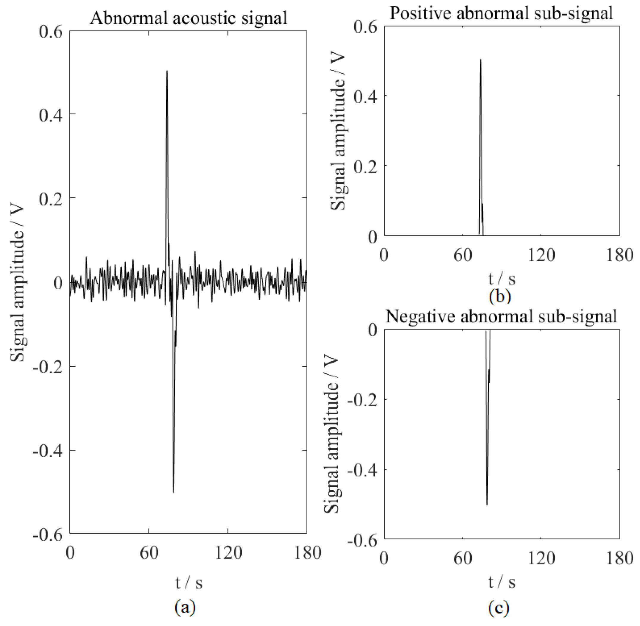
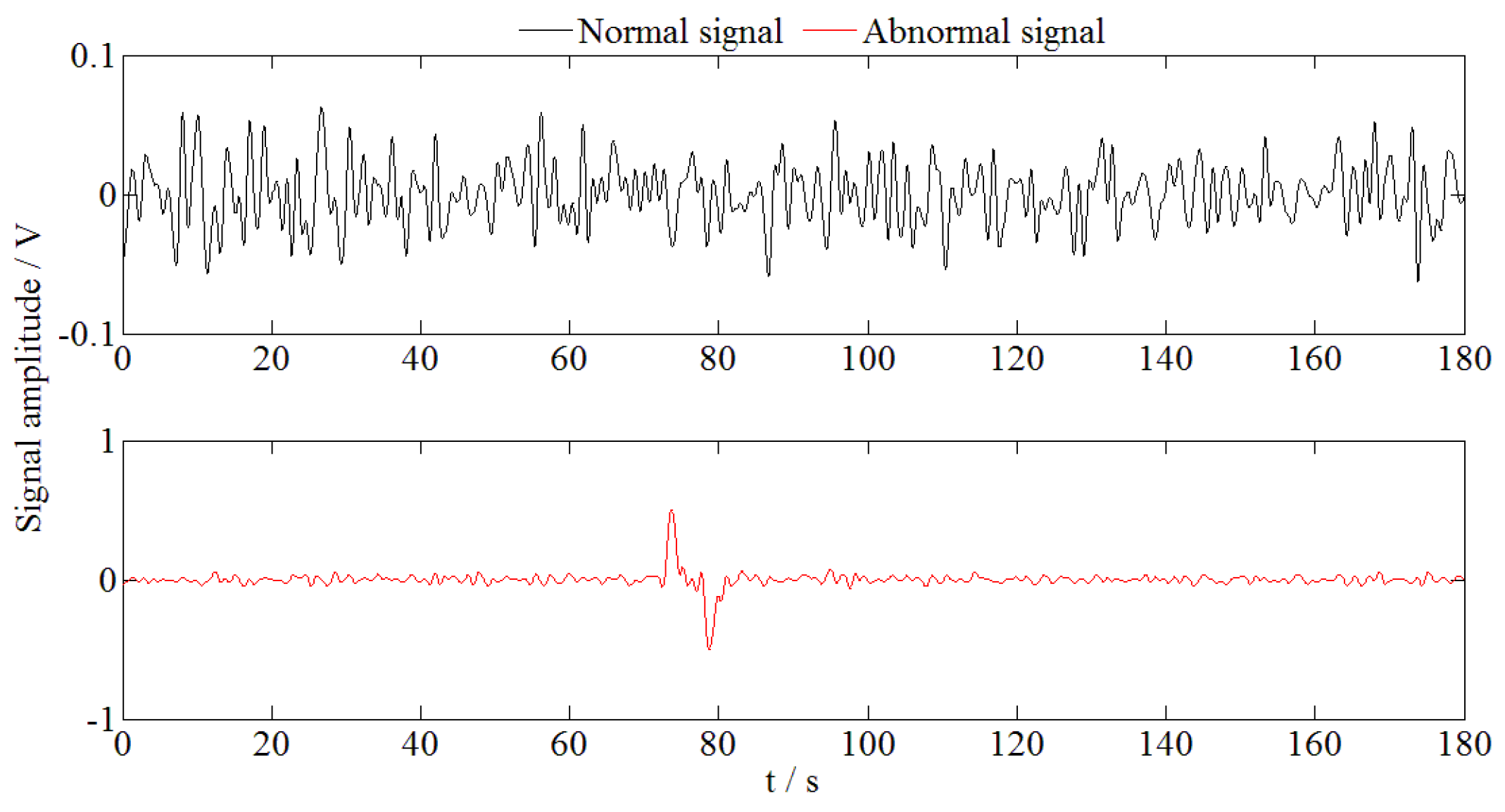
Figure 4 shows the decomposition diagram. The abnormal acoustic signal shown in Figure 5a was filtered with the Daubechies wavelet (wavelet basis: db 9, decomposition level: 5). In the absence of a special explanation, all acoustic signals in this study were filtered with the same setting of the wavelet. It is decomposed into 168 sub-signals; the 68nd sub-signal is a positive abnormal sub-signal (Figure 5b) and the corresponding starting time, ending time and peak value are 72.74 s, 75.62 s, 0.505 V, respectively; the 73th sub-signal is a negative abnormal sub-signal (Figure 5c) and its starting time, ending time and peak value are 77.88 s, 80.86 s and −0.503 V, respectively. The proposed decomposition method lays a good foundation for extracting local abnormal information in an acoustic signal.

3.2. Principle of the Model-Free Isolation Method

The peak sequence, composed of the peaks of all sub-signals in an acoustic signal, is denoted by ${\mathbf{A}}_{\mathrm{peak}}=[A_{\mathrm{peak}}\left(1\right),A_{\mathrm{peak}}\left(2\right),\dots ,A_{\mathrm{peak}}\left(j\right),\dots ,A_{\mathrm{peak}}\left(M\right)]$. All sub-signals are sorted from large to small according to their absolute peak value $|A_{\mathrm{peak}}\left(j\right)|$. Then, the ordered peak sequence is denoted by ${\mathbf{A}}_{\left|\mathrm{peak}\right|}=\left[\right|A_{\mathrm{peak}}\left(a_1\right)|,|A_{\mathrm{peak}}\left(a_2\right)|,\dots ,|A_{\mathrm{peak}}\left(a_j\right)|,\dots ,|A_{\mathrm{peak}}\left(a_M\right)\left|\right]$, where $a_j$ is the index of the sub-signal ${\mathbf{x}}_{\mathrm{sub}}\left(a_j\right)$ in the acoustic signal $\mathbf{x}$ and $a_j$ is an integer within the range of 1 to M.

The most intuitive difference between the abnormal and normal signals is that the former absolute peak is significantly larger than the latter [13,14] and the law is also suitable for abnormal and normal sub-signals. If there are m abnormal sub-signals in an acoustic signal, the sub-signals, corresponding to the first m peaks in the ordered peak sequence ${\mathbf{A}}_{\left|\mathrm{peak}\right|}$, are abnormal sub-signals. Based on the expert experience, the following lemmas can be summarized.

Lemma 1.

From a microscopic perspective, the absolute peaks in the sequence ${\mathit{A}}_{\left|\mathrm{peak}\right|}$ must be arranged from larger to small. That is, $|A_{\mathrm{peak}}\left(a_1\right)|>|A_{\mathrm{peak}}\left(a_2\right)|>\dots >|A_{\mathrm{peak}}\left(a_m\right)|>|A_{\mathrm{peak}}\left(a_{m+1}\right)|>|A_{\mathrm{peak}}\left(a_{m+2}\right)|>\dots >|A_{\mathrm{peak}}\left(a_M\right)|$.

Lemma 2.

From a macroscopic perspective, the absolute peak of the normal sub-signal is much smaller than that of the abnormal sub-signal and the normal sub-signals in the acoustic signal obeys the Gaussian distribution [14]. Therefore, the absolute peaks of normal sub-signals are approximately equal. That is, $|A_{\mathrm{peak}}\left(a_1\right)|>|A_{\mathrm{peak}}\left(a_2\right)|>\dots >|A_{\mathrm{peak}}\left(a_m\right)|\gg |A_{\mathrm{peak}}\left(a_{m+1}\right)|\approx |A_{\mathrm{peak}}\left(a_{m+2}\right)|\approx \dots \approx |A_{\mathrm{peak}}\left(a_M\right)|$.

Since the actual number m of abnormal sub-signals in an acoustic signal $\mathbf{x}$ to be detected is unknown, it can be assumed to be k whose value must be less than the number M of sub-signals. In order to make all equations meaningful (introduced in the following), its range is $k=1,2,\dots ,M-2$. Based on the SNR definition [29], the abnormal sub-signal is treated as the valid signal and the normal sub-signal as the background noise in an acoustic signal $\mathbf{x}$. Then, the SNR of the sub-signal ${\mathbf{x}}_{\mathrm{sub}}\left(a_j\right)$ is defined as follows:

$$S_k\left(a_j\right)=10\log \frac{{\left(A_{\mathrm{peak}}\left(a_j\right)\right)}^2/2}{{\sigma }_k^2}$$

(4)

where ${\sigma }_k$ is the standard deviation of peaks of all normal sub-signals in an acoustic signal (the number of abnormal sub-signals is k and the remaining ($M-k$) sub-signals are normal sub-signals) and it is described by:

$${\sigma }_k=\sqrt{\frac{1}{M-k}\sum _{j=k+1}^M{\left({|A}_{\mathrm{peak}}\left(a_j\right)|-\frac{1}{M-k}\sum _{j=k+1}^M{|A}_{\mathrm{peak}}\left(a_j\right)|\right)}^2}$$

(5)

In the case of $k=M$ or $k=M-1$, Equation (5) will be meaningless or make Equation (4) meaningless. Hence, the range of k ($k=1,2,\dots ,M-2$) is reasonable. As observed in Equations (4) and (5), the SNR $S_k\left(a_j\right)$ of the sub-signal ${\mathbf{x}}_{\mathrm{sub}}\left(a_j\right)$ changes with the number k of abnormal sub-signals, which indicates $S_k\left(a_j\right)$ is the function of k. Each k corresponds to an SNR sequence ${\mathbf{S}}_k=[S_k\left(a_1\right),S_k\left(a_2\right),\dots ,S_k\left(a_M\right)]$. The following three theorems can be deduced by analyzing Lemma 1 and Equation (4).

Theorem 1.

The SNR in the SNR sequence ${\mathit{S}}_k=[S_k\left(a_1\right),S_k\left(a_2\right),\dots ,S_k\left(a_M\right)]$ decreases in turn; that is, $S_k\left(a_j\right)>S_k\left(a_{j+1}\right)$.

Proof of Theorem 1.

According to $\mathbf{Lemma}\mathbf{1}$, the peak $|A_{\mathrm{peak}}\left(a_j\right)|$ is larger than the peak $|A_{\mathrm{peak}}\left(a_{j+1}\right)|$; therefore,

$$S_k\left(a_j\right)=10\log \frac{{\left(A_{\mathrm{peak}}\left(a_j\right)\right)}^2/2}{{\sigma }_k^2}>10\log \frac{{\left(A_{\mathrm{peak}}\left(a_{j+1}\right)\right)}^2/2}{{\sigma }_k^2}=S_k\left(a_{j+1}\right)$$

(6)

 □

Theorem 2.

The standard deviation ${\sigma }_k$ is a monotonically decreasing function of the number k of abnormal sub-signals: ${\sigma }_k>{\sigma }_{k+1}$.

Proof of Theorem 2.

First of all, the theorem is proved from the mathematical point of view. The average in Equation (5) is denoted by:

$${\mu }_k=\frac{1}{M-k}\sum _{j=k+1}^M|A_{\mathrm{peak}}\left(a_j\right)|$$

(7)

The difference between ${\mu }_k$ and ${\mu }_{k+1}$ is:

$$\begin{array}{cc}\hfill {\mu }_k-{\mu }_{k+1}& =\frac{1}{M-k}\sum _{j=k+1}^M|A_{\mathrm{peak}}\left(a_j\right)|-\frac{1}{M-k-1}\sum _{j=k+2}^M|A_{\mathrm{peak}}\left(a_j\right)|\hfill \\ & =\frac{1}{(M-k)(M-k-1)}\left[(M-k-1)\sum _{j=k+1}^M|A_{\mathrm{peak}}\left(a_j\right)|-(M-k)\sum _{j=k+2}^M|A_{\mathrm{peak}}\left(a_j\right)|\right]\hfill \\ & =\frac{1}{(M-k)(M-k-1)}\left[(M-k-1)|A_{\mathrm{peak}}\left(a_{k+1}\right)|-\sum _{j=k+2}^M|A_{\mathrm{peak}}\left(a_j\right)|\right]\hfill \\ & =\frac{1}{(M-k)(M-k-1)}\sum _{j=k+2}^M\left[|A_{\mathrm{peak}}\left(a_{k+1}\right)|-|A_{\mathrm{peak}}\left(a_j\right)|\right]\hfill \end{array}$$

(8)

As the peak sequence ${\mathbf{A}}_{\left|\mathrm{peak}\right|}$ is ordered from large to small, there is

$$|A_{\mathrm{peak}}\left(a_{k+1}\right)|>|A_{\mathrm{peak}}\left(a_{k+2}\right)|>\dots >|A_{\mathrm{peak}}\left(a_M\right)|$$

(9)

Hence, the $|A_{\mathrm{peak}}\left(a_{k+1}\right)|-|A_{\mathrm{peak}}\left(a_j\right)|$ in the Equation (8) is larger than 0. Combined with $k=1,2,\dots ,M-2$, the ${\mu }_k-{\mu }_{k+1}$ is larger than 0. Therefore, the ${\mu }_k$ is larger than ${\mu }_{k+1}$.

Then, the difference between ${\sigma }_k^2$ and ${\sigma }_{k+1}^2$ is:

$$\begin{array}{cc}\hfill {\sigma }_k^2-{\sigma }_{k+1}^2& =\frac{1}{M-k}\sum _{j=k+1}^M{\left(|A_{\mathrm{peak}}\left(a_j\right)|-{\mu }_k\right)}^2-\frac{1}{M-k-1}\sum _{j=k+2}^M{\left(|A_{\mathrm{peak}}\left(a_j\right)|-{\mu }_{k+1}\right)}^2\hfill \\ & =\frac{(M-k-1){\displaystyle \sum _{j=k+1}^M}{\left(|A_{\mathrm{peak}}\left(a_j\right)|-{\mu }_k\right)}^2-(M-k){\displaystyle \sum _{j=k+2}^M}{\left(|A_{\mathrm{peak}}\left(a_j\right)|-{\mu }_{k+1}\right)}^2}{(M-k)(M-k-1)}\hfill \end{array}$$

(10)

Since the ${\mu }_k$ is larger than ${\mu }_{k+1}$, Equation (10) can be rewritten as:

$$\begin{array}{cc}\hfill {\sigma }_k^2-{\sigma }_{k+1}^2& =\frac{(M-k-1){\displaystyle \sum _{j=k+1}^M}{\left(|A_{\mathrm{peak}}\left(a_j\right)|-{\mu }_k\right)}^2-(M-k){\displaystyle \sum _{j=k+2}^M}{\left(|A_{\mathrm{peak}}\left(a_j\right)|-{\mu }_{k+1}\right)}^2}{(M-k)(M-k-1)}\hfill \\ & >\frac{(M-k-1){\displaystyle \sum _{j=k+1}^M}{\left(|A_{\mathrm{peak}}\left(a_j\right)|-{\mu }_k\right)}^2-(M-k){\displaystyle \sum _{j=k+2}^M}{\left(|A_{\mathrm{peak}}\left(a_j\right)|-{\mu }_k\right)}^2}{(M-k)(M-k-1)}\hfill \\ & =\frac{(M-k-1){\left(|A_{\mathrm{peak}}\left(a_{k+1}\right)|-{\mu }_k\right)}^2-{\displaystyle \sum _{j=k+2}^M}{\left(|A_{\mathrm{peak}}\left(a_j\right)|-{\mu }_k\right)}^2}{(M-k)(M-k-1)}\hfill \\ & =\frac{{\displaystyle \sum _{j=k+2}^M}\left[{\left(|A_{\mathrm{peak}}\left(a_{k+1}\right)|-{\mu }_k\right)}^2-{\left(|A_{\mathrm{peak}}\left(a_j\right)|-{\mu }_k\right)}^2\right]}{(M-k)(M-k-1)}\hfill \\ & >0\hfill \end{array}$$

(11)

Hence ${\sigma }_k>{\sigma }_{k+1}$.

Then the theorem is proved from the physical point of view. When the number of abnormal sub-signals is k, ${\sigma }_k$ represents the standard deviation of peaks from $|A_{\mathrm{peak}}\left(a_{k+1}\right)|$ to $|A_{\mathrm{peak}}\left(a_M\right)|$ in the ordered peak sequence ${\mathbf{A}}_{\left|\mathrm{peak}\right|}$. When the number of abnormal sub-signals is $k+1$, ${\sigma }_{k+1}$ indicates the standard deviation from $|A_{\mathrm{peak}}\left(a_{k+2}\right)|$ to $|A_{\mathrm{peak}}\left(a_M\right)|$. Since $|A_{\mathrm{peak}}\left(a_{k+1}\right)|>|A_{\mathrm{peak}}\left(a_{k+2}\right)|$, the fluctuation of peaks used to calculate ${\sigma }_k$ is greater than that of peaks for calculating ${\sigma }_{k+1}$; that is, ${\sigma }_k>{\sigma }_{k+1}$. □

Theorem 3.

$S_{k+1}\left(a_1\right)-S_k\left(a_1\right)=S_{k+1}\left(a_2\right)-S_k\left(a_2\right)=\dots =S_{k+1}\left(a_j\right)-S_k\left(a_j\right)=\dots =S_{k+1}\left(a_M\right)-S_k\left(a_M\right)={\Delta }_k$, where ${\Delta }_k$ is a positive number and denoted by an SNR increment.

$${\Delta }_k=10\log \frac{{\sigma }_k^2}{{\sigma }_{k+1}^2}$$

(12)

Proof of Theorem 3.

According to the SNR definition (Equation (4)), the relationship between the $S_{k+1}\left(a_j\right)$ and $S_k\left(a_j\right)$ is:

$$\begin{array}{cc}\hfill S_{k+1}\left(a_j\right)-S_k\left(a_j\right)& =10\log \frac{{\left(A_{\mathrm{peak}}\left(a_j\right)\right)}^2/2}{{\sigma }_{k+1}^2}-10\log \frac{{\left(A_{\mathrm{peak}}\left(a_j\right)\right)}^2/2}{{\sigma }_k^2}\hfill \\ & =10\log \frac{{\sigma }_k^2}{{\sigma }_{k+1}^2}\hfill \\ & ={\Delta }_k\hfill \end{array}$$

(13)

From Theorem 2, it is known that ${\sigma }_k$ is larger than ${\sigma }_{k+1}$. Hence, ${\Delta }_k=10\log ({\sigma }_k^2/{\sigma }_{k+1}^2)>0$. Combined with Equation (13), Theorem 3 is proved. □

When the number of abnormal sub-signals is $k=1,2,\dots ,M-2$, the SNR increment sequence $\mathsf{\Delta }$ is:

$$\mathsf{\Delta }=[{\Delta }_1,{\Delta }_2,\dots ,{\Delta }_{M-3}]$$

(14)

According to Lemma 2 and Equation (5), if the actual number of abnormal sub-signals is m, then:

$${\sigma }_{m+1}\approx {\sigma }_{m+2}\approx \dots \approx {\sigma }_{M-2}$$

(15)

Hence,

$${\Delta }_{m+1}\approx {\Delta }_{m+2}\approx \dots \approx {\Delta }_{M-3}\approx 0$$

(16)

That indicates the SNR increment of normal sub-signals tends to zero. Therefore, the actual number m of abnormal sub-signals should satisfy:

$${\mathsf{\Delta }}_{m+1,\dots ,M-3}\to 0$$

(17)

In this paper, Equation (17) is realized by Equation (18). If $m=0$, the acoustic signal is a normal signal; otherwise, it is abnormal and has m abnormal sub-signals.

$$\sum _{k=m+1}^{M-3}\left[{\Delta }_k\right]=0$$

(18)

where $[·]$ represents the rounding function.

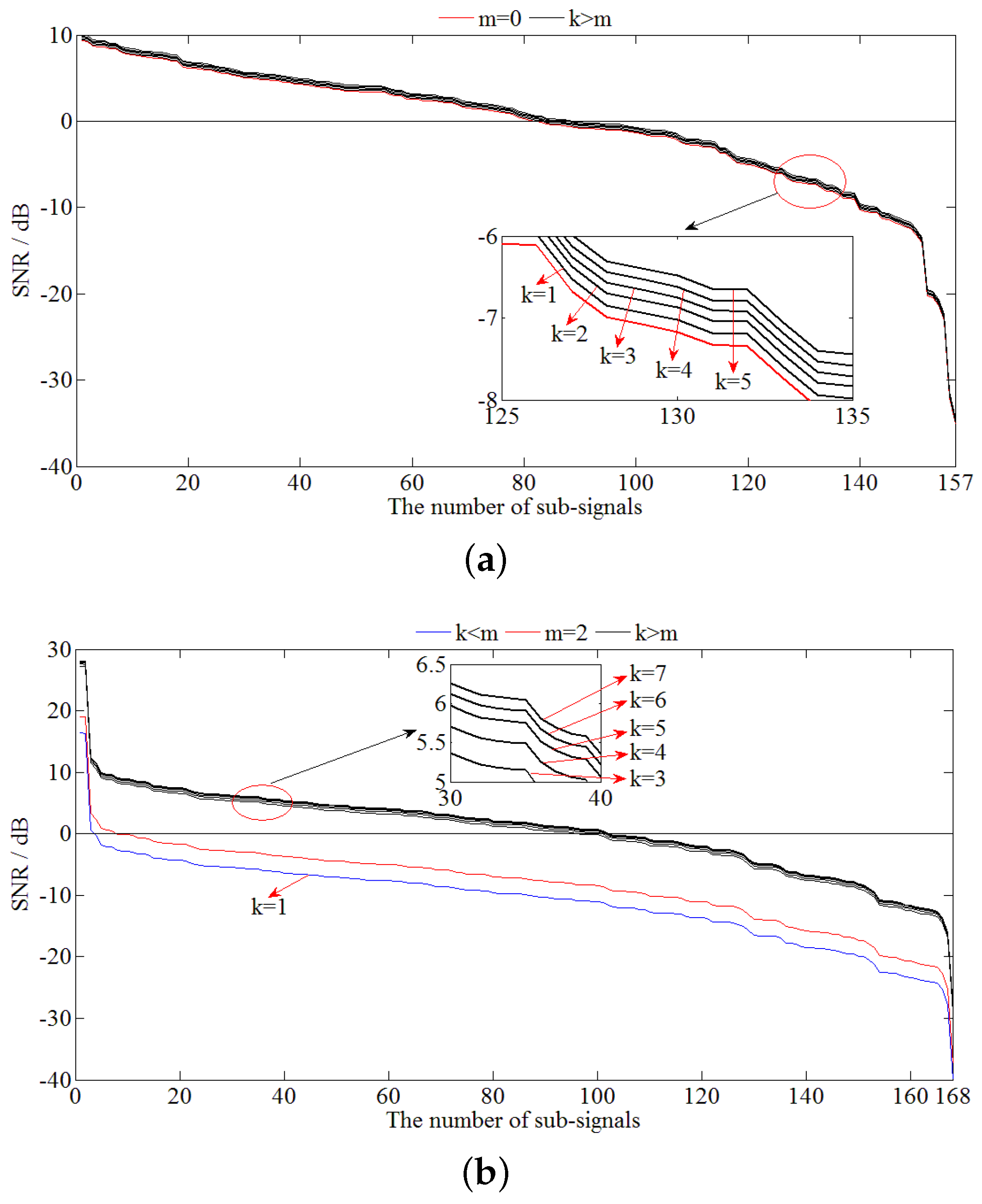
Figure 6 illustrates a normal and abnormal acoustic signal. According to the decomposition principle of an acoustic signal, the two signals are decomposed into 157 and 168 sub-signals and their actual numbers of abnormal sub-signals are $m=0$ and $m=2$, respectively.

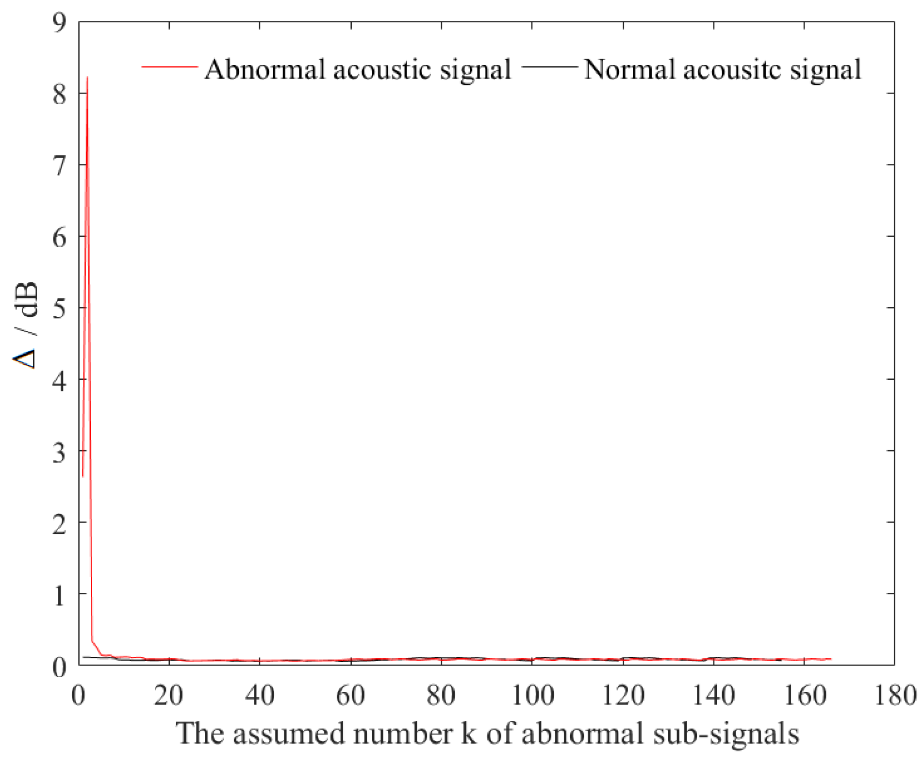
Their SNR distributions, varying along with the assumed number k of abnormal sub-signals, are illustrated in Figure 7a,b, respectively and the corresponding SNR increment sequences are illustrated in Figure 8. According to Equation (18), for the normal acoustic signal, its actual number m of abnormal sub-signals is 0 and the signal can be judged as a normal signal. Similarly, for the abnormal acoustic signal, it is judged as an abnormal signal and includes 2 abnormal sub-signals. Therefore, the diagnosis results are consistent with the actual situation.

3.3. Isolation of Abnormal Sub-Signals

While an acoustic signal is decomposed into M sub-signals, the index information, position information (starting time and end time) and peak information corresponding to each sub-signal are stored as follows:

$$\begin{array}{cc}\mathrm{Index}:\hfill & {\mathbf{I}}_{\mathrm{sub}}=[1,2,\dots ,j,\dots ,M]\hfill \\ \mathrm{Starting}\mathrm{time}:\hfill & {\mathbf{T}}_{\mathrm{start}}=[T_{\mathrm{start}}\left(1\right),T_{\mathrm{start}}\left(2\right),\dots ,T_{\mathrm{start}}\left(j\right),\dots ,T_{\mathrm{start}}\left(M\right)]\hfill \\ \mathrm{Ending}\mathrm{time}:\hfill & {\mathbf{T}}_{\mathrm{end}}=[T_{\mathrm{end}}\left(1\right),T_{\mathrm{end}}\left(2\right),\dots ,T_{\mathrm{end}}\left(j\right),\dots ,T_{\mathrm{end}}\left(M\right)]\hfill \\ \mathrm{Peak}:\hfill & {\mathbf{A}}_{\mathrm{peak}}=[A_{\mathrm{peak}}\left(1\right),A_{\mathrm{peak}}\left(2\right),\dots ,A_{\mathrm{peak}}\left(j\right),\dots ,A_{\mathrm{peak}}\left(M\right)]\hfill \end{array}$$

The sub-signals are sorted by the absolute peaks from large to small and the ordered peak sequence ${\mathbf{A}}_{\left|\mathrm{peak}\right|}$ and its index sequence ${\mathbf{I}}_{\left|\mathrm{sub}\right|}$ are:

$$\begin{array}{c}{\mathbf{A}}_{\left|\mathrm{peak}\right|}=\left[\right|A_{\mathrm{peak}}\left(a_1\right)|,|A_{\mathrm{peak}}\left(a_2\right)|,\dots ,|A_{\mathrm{peak}}\left(a_j\right)|,\dots ,|A_{\mathrm{peak}}\left(a_M\right)\left|\right]\\ {\mathbf{I}}_{\left|\mathrm{sub}\right|}=[a_1,a_2,\dots ,a_j,\dots ,a_M]\end{array}$$

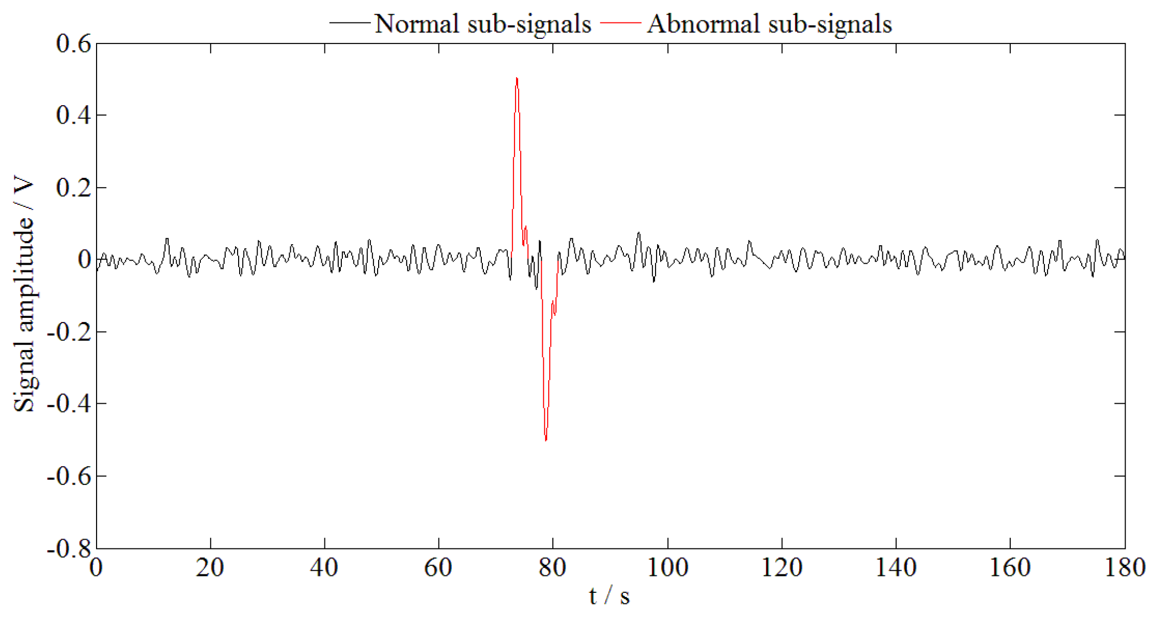
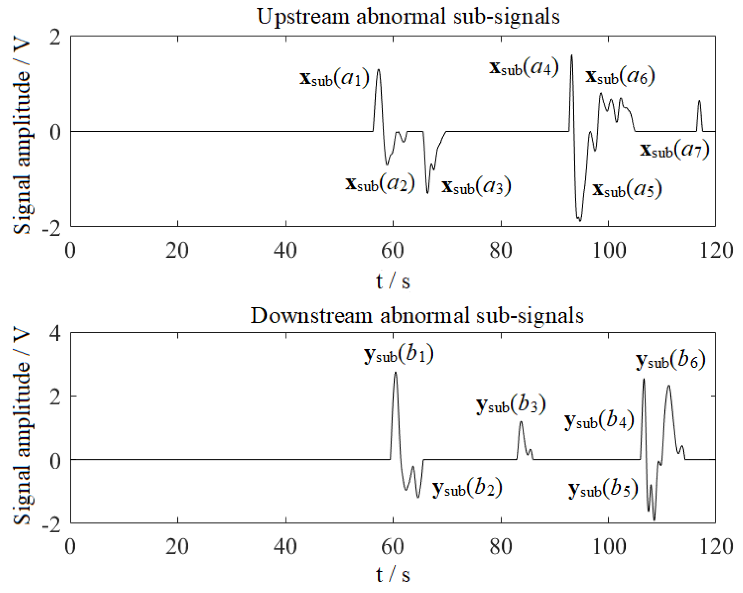
where $a_j$ is the index of the sub-signal ${\mathbf{x}}_{\mathrm{sub}}\left(a_j\right)$. Once the actual number m of abnormal sub-signals are known, the peaks of abnormal sub-signals are $A_{\mathrm{peak}}\left(a_1\right)\sim A_{\mathrm{peak}}\left(a_m\right)$. Hence, the indexes of abnormal sub-signals are $a_1\sim a_m$. According to these stored information (${\mathbf{I}}_{\mathrm{sub}},{\mathbf{T}}_{\mathrm{start}},{\mathbf{T}}_{\mathrm{end}}$) of sub-signals and the indexes $a_1\sim a_m$, each abnormal sub-signal can be isolated. Figure 9 shows the isolated abnormal sub-signals.

In summary, in the absence of feature extraction and a diagnosis model, the model-free isolation method can directly determine whether an acoustic signal is abnormal. Furthermore, the position of each abnormal sub-signal in the acoustic signal can be obtained, which provides the basis for the precise location of a leak. Figure 10 illustrates the detailed process of the model-free abnormal acoustic signal isolation method.

4. Leak Location

The classic location equation is [30]:

$$x_L=\frac{1}{2}\left(L+a\Delta t\right)$$

(19)

where $x_L$ is the distance from the leak point to the upstream acoustic sensor; a is the velocity of acoustic signals propagating inside the pipeline; L is the length between the upstream and downstream acoustic sensors; and $\Delta t$ is the time difference of the upstream and downstream leak signals, which can be calculated by Equations (20)–(22) and should satisfy Equation (23).

$$R_{xy}(\Delta n)=\underset{N\to +\infty }{\lim }\frac{1}{N}\sum _{i=1}^{N}x\left(i\right)y(i+\Delta n)$$

(20)

$$R_{xy}(\Delta n_0)=\max R_{xy}(\Delta n)$$

(21)

$$\Delta t=T\times \Delta n_0$$

(22)

$$-\frac{1}{a}(L+|l\left|\right)\le \Delta t\le \frac{1}{a}(L+|l\left|\right)$$

(23)

where $R_{xy}$ is the cross-correlation coefficient, $\Delta n$ is the delay points, $\Delta n_0$ is the delay points corresponding to the maximum of the cross-correlation coefficient $R_{xy}$, N is the data length of a signal, l is the allowable location error.

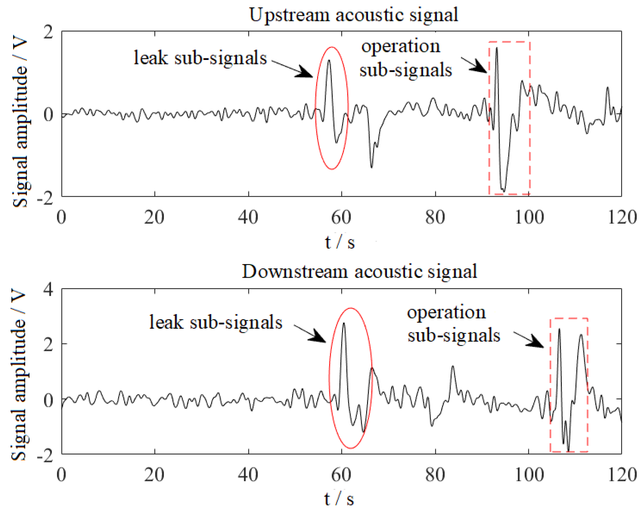
4.1. Analysis of the Influence of Operation Sub-Signals on Leak Location

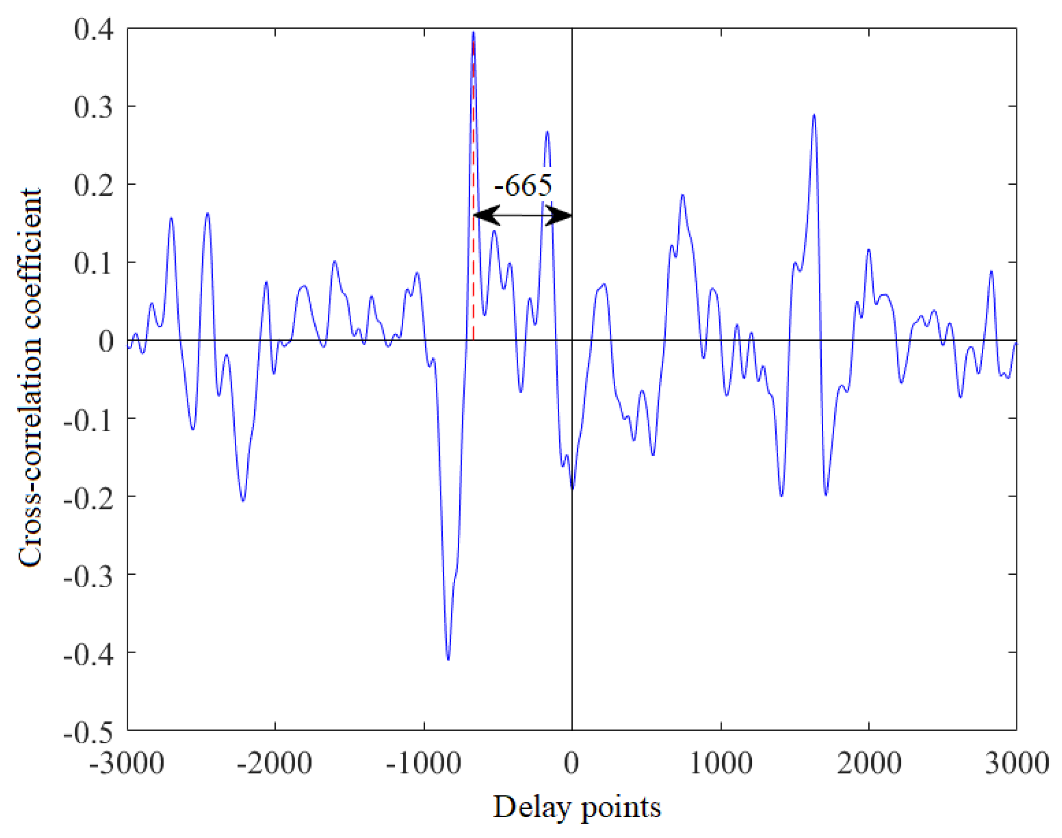
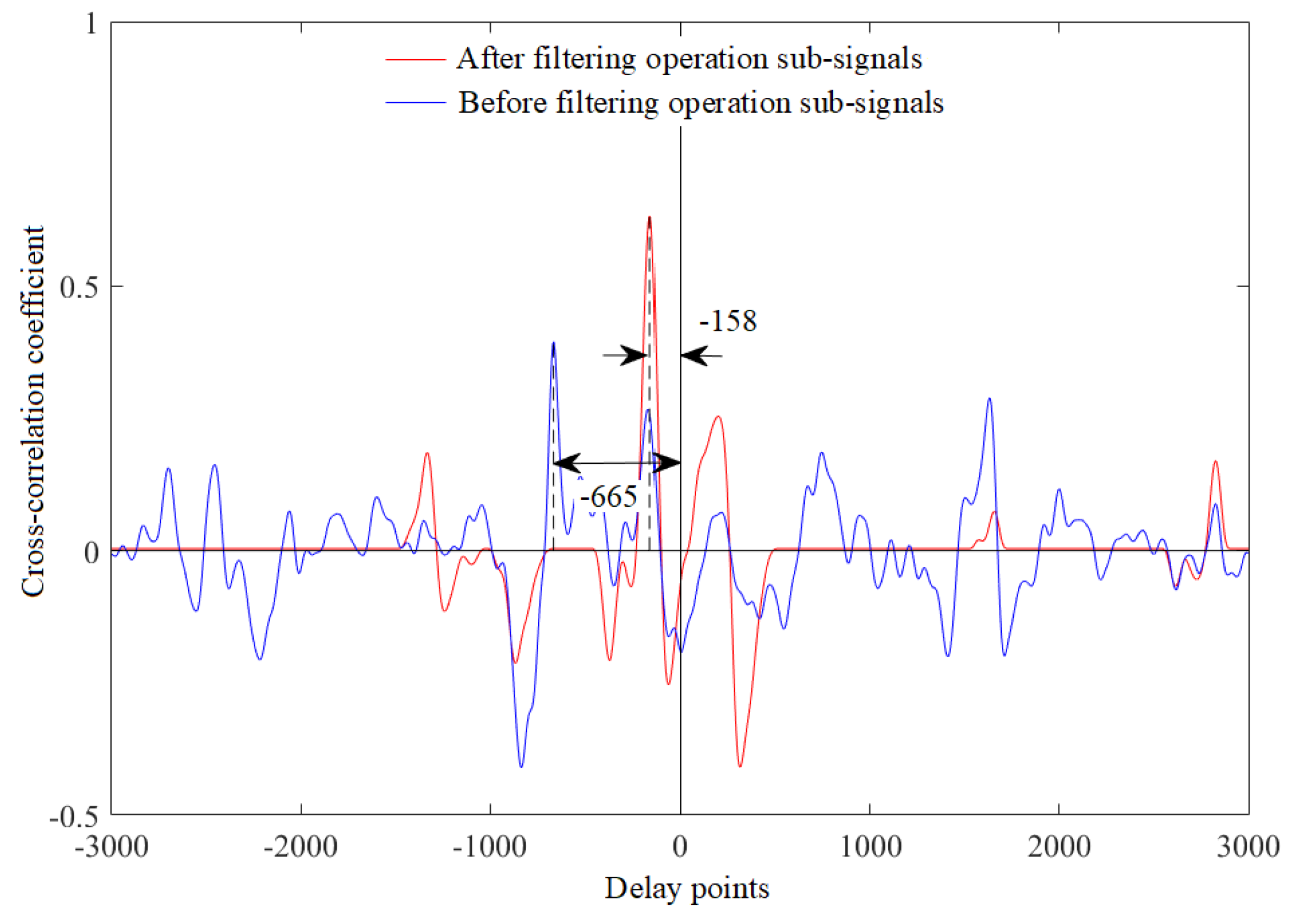
Figure 11 shows the abnormal acoustic signals containing both leak and operation sub-signals. When the whole signal is the object of cross-correlation analysis, the delay points are −665 (Figure 12). According to the sampling period $T=$0.02 s, the time difference $\Delta t$ is −13.3 s; combined with the total length of the pipeline $L=$15.6 km, the acoustic velocity $a=$1179 m/s and Equation (19), it locates at −0.0404 km from the upstream. However, the leak occurred at 6 km away from the upstream. Due to the influence of operation sub-signals, the leak is missing. Therefore, it is necessary to filter out operation sub-signals in an acoustic signal.

4.2. Leak Location Based on Filtering Operation Sub-Signals

The upstream acoustic signal is denoted by $\mathbf{x}=\left[x\right(1),x(2),\dots ,x(k),\dots ,x(N\left)\right]$ and the downstream is $\mathbf{y}=\left[y\right(1),y(2),\dots ,y(k),\dots ,y(N\left)\right]$. Based on the model-free isolation method (Section 3), the abnormal sub-signals of $\mathbf{x}$ and $\mathbf{y}$ can be isolated, they are denoted by (${\mathbf{x}}_{\mathrm{sub}}\left(a_1\right),{\mathbf{x}}_{\mathrm{sub}}\left(a_2\right),\dots ,{\mathbf{x}}_{\mathrm{sub}}\left(a_i\right),\dots ,{\mathbf{x}}_{\mathrm{sub}}\left(a_{mx}\right)$) and (${\mathbf{y}}_{\mathrm{sub}}\left(b_1\right),{\mathbf{y}}_{\mathrm{sub}}\left(b_2\right),\dots ,{\mathbf{y}}_{\mathrm{sub}}\left(b_j\right),\dots ,{\mathbf{y}}_{\mathrm{sub}}\left(b_{my}\right)$) and their number is $mx$ and $my$, respectively.

Taking abnormal sub-signals as the object, the two-two cross-correlation analysis of the same polarity abnormal sub-signals in the upstream and downstream signals is performed. When the upstream abnormal sub-signal ${\mathbf{x}}_{\mathrm{sub}}\left(a_i\right)$ and the downstream abnormal sub-signal ${\mathbf{y}}_{\mathrm{sub}}\left(b_j\right)$ are analyzed with cross-correlation calculation, in order to make data length consistent, the participating signals are:

$${\mathbf{X}}_i=\left\{X_i\left(k\right)|k=1,2,\dots ,N\right\},X_i\left(k\right)=\left\{\begin{array}{cc}x\left(k\right),\hfill & k\times T\in [T_{\mathrm{startx}}\left(a_i\right),T_{\mathrm{endx}}\left(a_i\right)]\hfill \\ 0,\hfill & \mathrm{others}\hfill \end{array}\right.$$

(24)

$${\mathbf{Y}}_j=\left\{Y_j\left(k\right)|k=1,2,\dots ,N\right\},Y_j\left(k\right)=\left\{\begin{array}{cc}y\left(k\right),\hfill & k\times T\in [T_{\mathrm{starty}}\left(b_j\right),T_{\mathrm{endy}}\left(b_j\right)]\hfill \\ 0,\hfill & \mathrm{others}\hfill \end{array}\right.$$

(25)

where $a_i$, $T_{\mathrm{startx}}\left(a_i\right)$ and $T_{\mathrm{endx}}\left(a_i\right)$ are the index, starting time and ending time of the abnormal sub-signal ${\mathbf{x}}_{\mathrm{sub}}\left(a_i\right)$ in the upstream acoustic signal $\mathbf{x}$; $b_j$, $T_{\mathrm{starty}}\left(b_j\right)$ and $T_{\mathrm{endy}}\left(b_j\right)$ are of the abnormal sub-signal ${\mathbf{y}}_{\mathrm{sub}}\left(b_i\right)$ in the downstream acoustic signal $\mathbf{y}$.

According to Equations (20) and (21), the delay points of the abnormal sub-signal ${\mathbf{X}}_i$ and ${\mathbf{Y}}_j$ are $\Delta n_{ij}$. The maximum and minimum time difference of an acoustic signal from upstream to downstream are $T_{\max }$ and $T_{\min }$, respectively.

$$T_{\max }=\frac{1}{a}(L+|l\left|\right),T_{\min }=\frac{1}{a}(L-|l\left|\right)$$

(26)

Since the operation sub-signals are generated by upstream or downstream, under the condition of ignoring the medium flow speed, if the time difference $\Delta t_{ij}$ satisfies Equation (27), the abnormal sub-signal ${\mathbf{x}}_{\mathrm{sub}}\left(a_i\right)$ and ${\mathbf{y}}_{\mathrm{sub}}\left(b_j\right)$ are operation sub-signals.

$$T_{\min }\le |\Delta t_{ij}=\Delta n_{ij}\times T|\le T_{\max }$$

(27)

Finally, filtering (${\mathbf{x}}_{\mathrm{sub}}\left(a_i\right)=0$, ${\mathbf{y}}_{\mathrm{sub}}\left(b_j\right)=0$) these operation sub-signals, their influence on leak location can be eliminated.

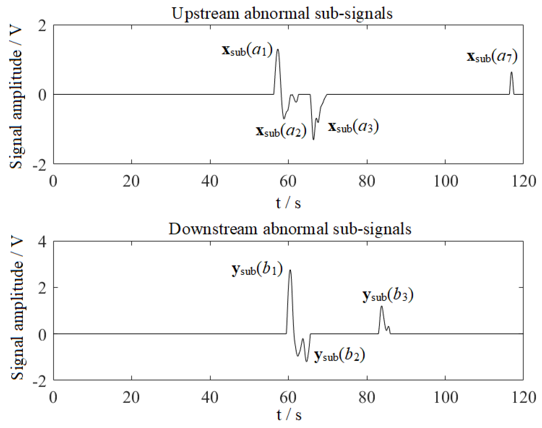
The upstream and downstream acoustic signals (Figure 11) are processed with the model-free isolation method described in Section 3 and the isolated abnormal sub-signals are shown in Figure 13.

Table 1. Time difference results of cross-correlation analysis of abnormal sub-signals.

Up/Down	${\mathbf{y}}_{\mathbf{sub}}\left({\mathit{b}}_1\right){|}_{+}$	${\mathbf{y}}_{\mathbf{sub}}\left({\mathit{b}}_2\right){|}_{-}$	${\mathbf{y}}_{\mathbf{sub}}\left({\mathit{b}}_3\right){|}_{+}$	${\mathbf{y}}_{\mathbf{sub}}\left({\mathit{b}}_4\right){|}_{+}$	${\mathbf{y}}_{\mathbf{sub}}\left({\mathit{b}}_5\right){|}_{-}$	${\mathbf{y}}_{\mathbf{sub}}\left({\mathit{b}}_6\right){|}_{+}$
${\mathbf{x}}_{\mathrm{sub}}\left(a_1\right){|}_{+}$	−3.16 s	--	×	×	--	×
${\mathbf{x}}_{\mathrm{sub}}\left(a_2\right){|}_{-}$	--	−3.16 s	--	--	×	--
${\mathbf{x}}_{\mathrm{sub}}\left(a_3\right){|}_{-}$	--	3.98 s	--	--	×	--
${\mathbf{x}}_{\mathrm{sub}}\left(a_4\right){|}_{+}$	×	--	11.73 s	−13.38 s	--	×
${\mathbf{x}}_{\mathrm{sub}}\left(a_5\right){|}_{-}$	--	×	--	--	−13.36 s	--
${\mathbf{x}}_{\mathrm{sub}}\left(a_6\right){|}_{+}$	×	--	×	−7.82 s	--	−13.14 s
${\mathbf{x}}_{\mathrm{sub}}\left(a_7\right){|}_{+}$	×	--	×	10.38 s	--	5.74 s

Symbol “+” represents that the polarity of a abnormal sub-signal is positive. Symbol “−” represents that the polarity of a abnormal sub-signal is negative. Symbol “×” represents that time difference does not satisfy Equation (23). Symbol “--” represents that abnormal sub-signals do not belong to the same polarity and should not be subjected to the cross-correlation analysis.

shows the time difference of abnormal sub-signals. According to the pipeline length $L=$ 15.6 km, the propagation velocity $a=$ 1179 m/s, the allowable location error $l=\pm$200 m and Equation (26), the time difference $\Delta t$ of operation sub-signals (Figure 13) should be in the range [13.06 s, 13.40 s]∪[−13.40 s, −13.06 s]. In Table 1, there are three pair abnormal sub-signals ($({\mathbf{x}}_{\mathrm{sub}}\left(a_4\right),{\mathbf{y}}_{\mathrm{sub}}\left(b_4\right))$, $({\mathbf{x}}_{\mathrm{sub}}\left(a_5\right),{\mathbf{y}}_{\mathrm{sub}}\left(b_5\right))$ and $({\mathbf{x}}_{\mathrm{sub}}\left(a_6\right),{\mathbf{y}}_{\mathrm{sub}}\left(b_6\right))$) whose time difference is within the range. Therefore, they are operation sub-signals. After these operation signals are filtered, the remaining abnormal sub-signals are shown in Figure 14.

The comparison of the cross-correlation analysis of the acoustic signals, before and after operation sub-signals are filtered, is further plotted in Figure 15. As shown, after filtering operation sub-signals, the delay points $\Delta n_0$ has changed from −665 to −158, the time difference $\Delta t$ becomes 3.16 s, the leak location $x_L$ is 5.937 km and the location error is 63 m. Therefore, the accurate alarm for the leak is achieved after filtering operation sub-signals.

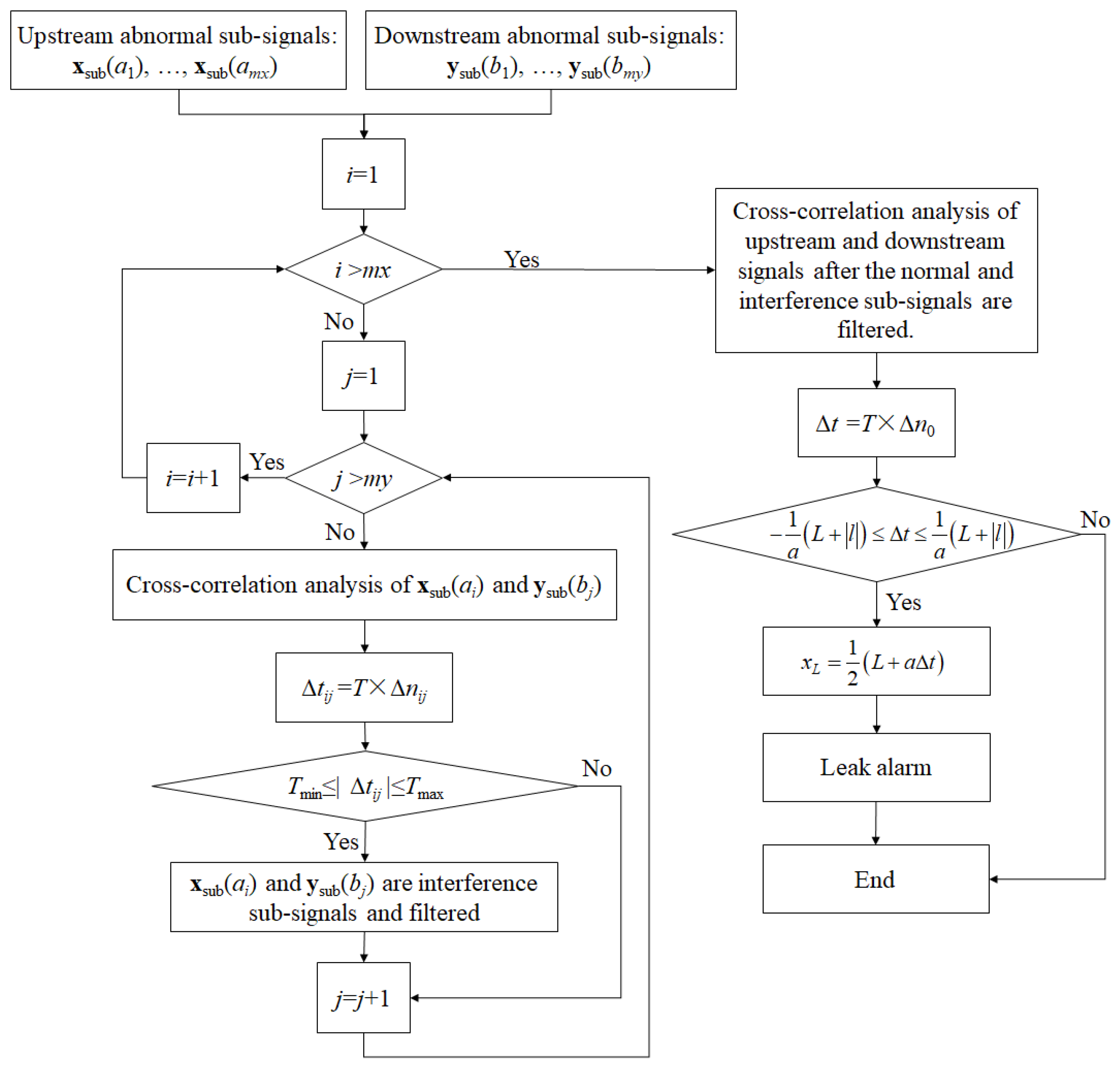
In summary, the combination of the model-free isolation method and the filtering operation sub-signals method realizes accurate detection and location of a pipeline leak. The specific process of leak location is shown in Figure 16.

5. Experimental Results

The validity of the proposed method was verified with the historical data of a naphtha pipeline and a crude oil pipeline, the specific parameters of which are given in

Table 2. Parameters of the naphtha and crude oil pipeline.

Parameters	Value/Unit
	Naphtha	Crude oil
Total length	15.511 km	15.600 km
Pipeline diameter	150 mm	250 mm
Pipeline thickness	6 mm	unknown
Fluid density	0.76 g· cm${}^{-3}$	0.86 g· cm${}^{-3}$
Acoustic velocity	1055 m· s${}^{-1}$	1179 m· s${}^{-1}$
Upstream pressure	2.18 MPa	2.80 MPa
Downstream pressure	0.48 MPa	0.67 MPa
Leak point to upstream	9.476 km	6.000 km
Leak aperture	<4 mm, 4 mm, <8 mm, 8 mm	4 mm
Pipeline material	metal
Sampling frequency	50 Hz
Sampling precision	12 bit A/D

. All leaks used in this paper were artificially generated by the cooperative unit opening a valve and only the case of a single leak is considered. On the naphtha pipeline, the cooperative unit carried out 15 leak experiments on 20–21 November 2013, respectively. On the crude oil pipeline, there were 6 leaks on 27 March 2011; because of the conveying process, these leak signals contain many operation sub-signals.

5.1. Field Test

Based on the proposed leak detection method,

Table 3. Location results before and after filtering operation sub-signals.

Pipeline	Sample	Location (km)
		Before	After
Naphtha	1	9.496	9.496
	2	9.444	9.444
	3	9.496	9.496
	4	9.512	9.512
	5	9.507	9.507
	6	9.496	9.496
	7	9.444	9.444
	8	9.475	9.475
	9	9.438	9.438
	10	9.444	9.444
	11	9.475	9.475
	12	9.517	9.517
	13	9.465	9.465
	14	9.517	9.517
	15	9.507	9.507
Crude oil	1	−0.116	5.981
	2	−0.152	5.957
	3	−0.069	5.946
	4	−0.042	5.934
	5	5.364	5.840
	6	−0.140	5.946

shows the leak location results before and after operation sub-signals are filtered. For the naphtha pipeline, the locations are the same before and after filtering operation sub-signals since the 15 leak signals do not contain operation sub-signals and the maximum location is 41 m. For the crude oil pipeline, after filtering operation sub-signals, the missing alarms change from 83.33% (5/6) to 0 and the maximum location error change from 636 m to 160 m. Therefore, it demonstrates that the leak detection method, based on the model-free isolation of abnormal signals and the filtering operation sub-signals, is valid.

5.2. Comparison of Methods

Based on the historical data from the naphtha pipeline (20–21 November 2013) and the crude oil pipeline (26–27 March 2011), the WPE-based leak detection [15] and SVDD-based leak diagnosis [14] methods were compared with the method proposed in this paper. The comparisons were made from three perspectives: (1) the running time of one complete diagnosis with the same operating environment (Lenovo laptop of 8 GB memory and Matlab 2013a); (2) the number of false and missing alarms; and (3) the largest location error. The parameters used in the WPE-based and SVDD-based diagnosis modeling methods are implemented as follows:

• WPE. Wavelet basis function: Daubechies 1 wavelet (db 1); decomposition level: 5; window width: 100; sliding step length: 10.
• SVDD.Group number: 200; feature-frequency: 0.1, 0.2, 0.3, 0.4, 0.5, 0.6, 0.7; Gaussian kernel function: ${\sigma }_{\mathrm{svdd}}$ = 0.28.

The comparison results are given in

Table 4. Comparison of offline test between the model-free-based (proposed), support vector domain description (SVDD)-based and WPE-based methods on the naphtha pipeline.

Pipeline	Method	Running Time (s)	Number of Alarms			Largest Location Error (m)
			Leak	False	Missing
Naphtha	Model-free	$0.041$	15	0	0	41
	SVDD	$0.083$	15	0	0	64
	WPE	$53.187$	13	4	2	64
Crude oil	Model-free	$0.041$	6	0	0	160
	SVDD	$0.083$	1	1	5	636
	WPE	$53.187$	1	3	5	636

. It can be observed that: (1) the proposed method required the shortest running time to complete a diagnosis, had no missing and false alarms and had the smallest location error; (2) for the naphtha pipeline, the SVDD-based method did not report missing and false alarms but it had 1 false alarm and 5 missing alarms for the crude oil pipeline; and (3) the WPE-based method had both false and missing alarms for the two pipelines.

Based on the above, it can be concluded that the proposed method could achieve pipeline leak detection without a diagnosis model compared to existing methods, reduced the running time, improved location accuracy and did not produce missing alarms.

6. Conclusions

A pipeline leak detection and location method based on model-free abnormal acoustic signal isolation is proposed in this paper. By decomposing the acoustic signal into sub-signals, the functional relationship between a sub-signal SNR and the number of abnormal sub-signals was established. The actual number m of abnormal sub-signals can be calculated according to the SNR increment and the position of each abnormal sub-signal in the acoustic signal can be traced by its index. Finally, based on the cross-correlation analysis, the precise location of leaks is achieved by filtering operation sub-signals. The proposed method does not require feature extraction or a diagnosis model and reduce the impact of operation sub-signals on leak location and the experimental results indicated that the method does not produce any missing and false alarms as well as provides higher location precision compared with other methods.

References

- Zhe, L.; Yuntong, S.; Mark, L. A Sensitivity Analysis of a Computer Model-Based Leak Detection System for Oil Pipelines. Energies 2017, 10, 1226. [Google Scholar] [CrossRef]
- Breton, T.; Sanchez-Gheno, J.C.; Alamilla, J.L.; Alvarez-Ramirez, J. Identification of Failure Type in Corroded Pipelines: A Bayesian Probabilistic Approach. J. Hazard. Mater. 2010, 179, 628–634. [Google Scholar] [CrossRef] [PubMed]
- He, G.; Liang, Y.; Li, Y.; Wu, M.; Sun, L.; Xie, C.; Li, F. A Method for Simulating the Entire Leaking Process and Calculating the Liquid Leakage Volume of a Damaged Pressurized Pipeline. J. Hazard. Mater. 2017, 332, 19–32. [Google Scholar] [CrossRef] [PubMed]
- Taghvaei, M.; Beck, S.B.M.; Staszewski, W.J. Leak Detection in Pipelines Using Cepstrum Analysis. Meas. Sci. Technol. 2006, 17, 367–372. [Google Scholar] [CrossRef]
- Wang, X.; Ghidaoui, M.S. Identification of Multiple Leaks in Pipeline: Linearized Model, Maximum Likelihood, and Super-resolution Localization. Mech. Syst. Signal Process. 2018, 107, 529–548. [Google Scholar] [CrossRef]
- Qu, Z.; Wang, Y.; Yue, H.; An, Y.; Wu, L.; Zhou, W.; Wang, H.; Su, Z.; Li, J.; Zhang, Y.; et al. Study on the Natural Gas Pipeline Safety Monitoring Technique and the Time-frequency Signal Analysis Method. J. Loss Prev. Process Ind. 2017, 47, 1–9. [Google Scholar] [CrossRef]
- Cataldo, A.; Cannazza, G.; De Benedetto, E.; Giaquinto, N. A TDR-based System for the Localization of Leaks in Newly Installed, Underground Pipes Made of Any Material. Meas. Sci. Technol. 2012, 23, 105010. [Google Scholar] [CrossRef]
- Thang Bui, Q.; Sohaib, M.; Jong-Myon, K. A Reliable Acoustic EMISSION Based Technique for the Detection of a Small Leak in a Pipeline System. Energies 2019, 12, 1472. [Google Scholar] [CrossRef]
- Liu, C.; Li, Y.; Fu, J.; Liu, G. Experimental Study on Acoustic Propagation-characteristics-based Leak Location Method for Natural Gas Pipelines. Process Saf. Environ. Prot. 2015, 96, 43–60. [Google Scholar] [CrossRef]
- Yu, X.; Liang, W.; Zhang, L.; Jin, H.; Qiu, J. Dual-tree Complex Wavelet Transform and SVD Based Acoustic Noise Reduction and its Application in Leak Detection for Natural Gas Pipeline. Mech. Syst. Signal Process. 2016, 72–73, 266–285. [Google Scholar] [CrossRef]
- Di, L.; Jianchun, F.; Shengnan, W. Acoustic Wave-Based Method of Locating Tubing Leakage for Offshore GasWells. Energies 2018, 11, 3454. [Google Scholar] [CrossRef]
- Sepideh, Y.; Kalyan, R.P.; Sez, A.; Abdul, K. Experimental evaluation of a vibration-based leak detection technique for water pipelines. Struct. Infrastruct. Eng. 2018, 14, 46–55. [Google Scholar] [CrossRef]
- Xu, Q.; Zhang, L.; Liang, W. Acoustic Detection Technology for Gas Pipeline Leakage. Process Saf. Environ. Prot. 2013, 91, 253–261. [Google Scholar] [CrossRef]
- Wang, F.; Lin, W.; Liu, Z.; Wu, S.; Qiu, X. Pipeline Leak Detection by Using Time-Domain Statistical Features. IEEE Sens. J. 2017, 17, 6431–6442. [Google Scholar] [CrossRef]
- Zhang, Y.; Chen, S.; Li, J.; Jin, S. Leak Detection Monitoring System of Long Distance Oil Pipeline Based on Dynamic Pressure Transmitter. Measurement 2014, 49, 382–389. [Google Scholar] [CrossRef]
- Sun, J.; Xiao, Q.; Wen, J.; Zhang, Y. Natural Gas Pipeline Leak Aperture Identification and Location Based on Local Mean Decomposition Analysis. Measurement 2016, 79, 147–157. [Google Scholar] [CrossRef]
- Tax, D.M.J.; Duin, R.P.W. Support Vector Data Description. Mach. Learn. 2004, 54, 45–66. [Google Scholar] [CrossRef] [Green Version]
- Zheng, S. Smoothly Approximated Support Vector Domain Description. Pattern Recognit. 2016, 49, 55–64. [Google Scholar] [CrossRef]
- Roodposhti, M.S.; Safarrad, T.; Shahabi, H. Drought Sensitivity Mapping Using Two One-class Support Vector Machine Algorithms. Atmos. Res. 2017, 193, 73–82. [Google Scholar] [CrossRef]
- Sameh, S.; Zied, L. Audio Sounds Classification Using Scattering Features and Support Vectors Machines for Medical Surveillance. Appl. Acoust. 2018, 30, 270–282. [Google Scholar] [CrossRef]
- Wang, S.; Gao, R.; Wang, L. Bayesian Network Classifiers Based on Gaussian Kernel Density. Expert Syst. Appl. 2016, 51, 207–217. [Google Scholar] [CrossRef]
- Lin, W.; Xiaodong, W.; Fenwei, W.; Wu, H. Feature Extraction and Early Warning of Agglomeration in Fluidized Bed Reactors Based on an Acoustic Approach. Powder Technol. 2015, 279, 185–195. [Google Scholar] [CrossRef]
- Mandal, S.K.; Chan, F.T.; Tiwari, M.K. Leak Detection of Pipeline: An Integrated Approach of Rough Set Theory and Artificial Bee Colony Trained SVM. Expert Syst. Appl. 2012, 39, 3071–3080. [Google Scholar] [CrossRef]
- Soldevila, A.; Fernandez-Canti, R.M.; Blesa, J.; Tornil-Sin, S.; Puig, V. Leak Localization in Water Distribution Networks Using Bayesian Classifiers. J. Process Control 2017, 55, 1–9. [Google Scholar] [CrossRef]
- El-Zahab, S.; Abdelkader, E.M.; Zayed, T. An accelerometer-based leak detection system. Mech. Syst. Signal Process. 2018, 108, 276–291. [Google Scholar] [CrossRef]
- Liu, C.; Li, Y.; Fang, L.; Xu, M. Experimental Study on a De-noising System for Gas and Oil Pipelines Based on an Acoustic Leak Detection and Location Method. Int. J. Press. Vessel. Pip. 2017, 151, 20–34. [Google Scholar] [CrossRef]
- Wang, J.; Zhao, L.; Liu, T.; Li, Z.; Sun, T.; Grattan, K.T.V. Novel Negative Pressure Wave-based Pipeline Leak Detection System Using Fiber Bragg Grating-based Pressure Sensors. J. Lightwave Technol. 2017, 35, 3366–3373. [Google Scholar] [CrossRef]
- Alberto, M.; Alessandro, R.; Marco, T. Autocorrelation Analysis of Vibro-Acoustic Signals Measured in a Test Field for Water Leak Detection. Appl. Sci. 2018, 8, 2450. [Google Scholar] [CrossRef]
- Ozdemir, G.; Maghsoodloo, S. Quadratic Quality Loss Functions and Signal-to-noise Ratios for a Trivariate Response. J. Manuf. Syst. 2004, 23, 144–171. [Google Scholar] [CrossRef]
- Gao, Y.; Brennan, M.J.; Liu, Y.; Almeida, F.C.; Joseph, P.F. Improving the Shape of the Cross-correlation Function for Leak Detection in a Plastic Water Distribution Pipe Using Acoustic Signals. Appl. Acoust. 2017, 127, 24–33. [Google Scholar] [CrossRef]
Figure 1.
System architecture for the acoustic sensor-based leak detection.
Figure 2.
The configuration of the acoustic transducer.
Figure 3.
Field installation of the acoustic transducers on pipelines.
Figure 4.
Signal decomposition diagram.
Figure 5.
Decomposition example of an acoustic signal.
Figure 6.
Time domain waveform of normal and abnormal acoustic signals.
Figure 7.
The signal to noise ration (SNR) sequence of normal and abnormal acoustic signals varies with the number k of abnormal sub-signals. (a) Normal acoustic signal: the actual number of abnormal sub-signals is m = 0. (b) Abnormal acoustic signal: the actual number of abnormal sub-signals is m = 2.
Figure 8.
SNR increment sequence .
Figure 9.
Time domain waveform of abnormal sub-signals isolated from the acoustic signal.
Figure 10.
Flow chart of the model-free abnormal acoustic signal isolation method.
Figure 11.
Abnormal signal example with leak and operation sub-signals.
Figure 12.
Cross-correlation analysis of the abnormal signals.
Figure 13.
Isolated abnormal sub-signals.
Figure 14.
Abnormal sub-signals after filtering operation sub-signals.
Figure 15.
Cross-correlation curves before and after filtering operation sub-signals.
Figure 16.
Flow chart of the leak location method based on filtering operation sub-signals.