Research on an Asymmetric Fault Control Strategy for an AC/AC System Based on a Modular Multilevel Matrix Converter

Abstract

This paper studies control strategies for an AC/AC system based on a modular multilevel matrix converter (M³C) when an asymmetric fault occurs in the secondary side ac system. Firstly, the operating principle of M³C is briefly introduced and verified by simulation. Then, based on its mathematical model by double αβ0 transformation, the decoupled control strategies for the primary side and secondary side systems are designed. In view of the asymmetric fault condition of the secondary side system, the positive sequence and negative sequence components of voltages and currents are separated and extracted, and then a proportional resonant controller (PR) is used to regulate the positive and negative sequence currents at the same time to realize decoupled current control in the αβ reference frames. The capacitor voltage balancing control, which consists of an inter-subconverter balancing control and an inner-subconverter balancing control, is realized by adjusting four circulating currents. Finally, the proposed control strategy is validated by simulation in the PSCAD/EMTDC software (Manitoba HVDC Research Center, Canada). The result shows that during the period of the BC-phase short-circuit fault occurring in the secondary side system, the whole system can still operate stably and transmit a certain amount of active power, according to their set values. Furthermore, the capacitor voltages are balanced, with a slight increase during the fault period. The simulation results verify the effectiveness of the proposed control strategy.

1. Introduction

As a new type of voltage source converter, the modular multilevel converter (MMC) has attracted wide attention and research in both academia and industry since it was proposed by German scholar R. Marquardt in 2001 [1]. Due to the MMC’s advantages, such as its modular structure, high quality voltage and current waveforms, fault tolerance, and redundancy control, an MMC with a back-to-back configuration (BTB-MMC) is widely used in voltage sourced converter high voltage direct current (VSC-HVDC) transmission systems.

Similar to BTB-MMC, which can connect two AC systems with different frequencies, modular multilevel direct AC/AC converters have been proposed in recent years. For example, the Modular Multilevel Matrix Converter (MMMC or M³C) [2,3], which consists of nine branches, each comprising several series-connected H-bridge submodules and an inductor, is suitable for a 3Φ-to-3Φ AC/AC bidirectional power conversion. In addition, large capacity AC/AC converters are needed in many applications, such as the asynchronous interconnection of different power systems and medium or high voltage motor drives. For these applications, an indirect AC/DC/AC converter with a back-to-back structure is usually employed, and a large DC link capacitor is needed in the intermediate stage. At present, the most widely used direct AC/AC converters are mainly thyristor based cycloconverters and matrix converters [4]. These two converters are attractive because they lack a DC link or DC filter. However, the shortcomings of these two converters are also obvious. For cycloconverters, in order to ensure the quality of their output voltage waveform, their frequency conversion is limited, that is, the ratio of the output to input frequency should be less than one third to reduce harmonics. In addition, the power factor of a cycloconverter is low, and its harmonics are large, which requires a large amount of reactive power compensation, as well asfiltering devices. For a matrix converter, although its output frequency and power factor are arbitrarily adjustable, the chopper mode limits its voltage utilization, and additional step-up transformers are often needed in practical applications. Thus, there are two problems. Firstly, the utilization of voltage is low, and transformers are needed to boost the output voltage. Secondly, it is difficult to realize high voltage and a large capacity because the bidirectional switch of the matrix converter is only composed of semiconductor switch devices. Therefore, from the viewpoint of overcoming the above shortcomings of both converters, the M³C is a promising structure for high capacity direct AC/AC converters.

Up to now, the application of M³Cs has mainly focused on medium voltage and high-power AC variable frequency speed regulation and power electronic transformers [5,6,7,8,9,10,11,12,13,14]. Since 2013, some scholars have proposed the application of M³C to the field of low frequency AC transmission (LFAC) and have undertaken preliminary studies on its control strategy [15,16,17,18]. The control of an M³C is very complex and has two main technical problems. Firstly, the converter has more degrees of freedom (nine voltage and eight current degrees of freedom, to be exactly), so it is difficult to achieve independent control for each degree of freedom. Secondly, due to the different frequencies of both sides systems, the converter’s branch currents consist of different frequency components. Thus, the strong coupling between these components yields great challenges to control methods. Additionally, like the other modular multilevel converter, M³C’s numerous floating capacitors will inevitably suffer from the unbalanced capacitor voltage caused by the differences in the triggering process and capacitance parameter of each submodule. Therefore, appropriate capacitor voltage balancing control methods are needed to ensure the stable operation of the converter. The most widely used decoupling control methods for M³C are based on double αβ0 coordinate transformation [9,10,11,19,20,21]. By applying double αβ0 transformation to M³C, not only can the mathematical model of M³C be simplified, but the decoupling control between different degrees of freedom can also be realized.

Furthermore, whether in motor driving or low frequency AC transmission applications, the power systems often exist in asymmetric operation conditions due to sudden faults, such as single-phase short-circuit faults in the AC system. When the three-phase systems are asymmetric, the negative sequence components of the electrical quantities will appear and will increase the RMS value of the currents, which will lead to overcurrent in the system. At the same time, a large number of non-characteristic harmonics will be generated on both sides of the M³C system. These harmonics may have an effect on the controller, deteriorate the control results, and also lead to overcurrent of the devices in the converter, or even burn down the components, which will seriously endanger the safe and stable operation of the whole system. Therefore, it is necessary to study the control strategy of an AC/AC system based on M³C under asymmetric fault conditions.

In this paper, an asymmetric fault control strategy for an AC/AC system based on a modular multilevel matrix converter is proposed. Firstly, the structure and operating principles of the M³C are introduced and simulated. Then, based on the mathematical model of the αβ reference frames, control strategies for primary side system and secondary side system are proposed. In light of the asymmetric fault conditions that occur in the secondary side system, the positive and negative sequence components of voltages and currents are separated, and then the proportional resonant controller (PR) is used to regulate the positive and negative sequence components at the same time to realize decoupled control in its αβ reference frames. Finally, a case is given to confirm the effectiveness of the proposed control strategy under the condition that a short-circuit fault between the BC-phase occurs in the secondary side system. The simulation results validate that the proposed control strategy can ensure stable operation of the systems under asymmetric fault conditions.

2. System Configuration and Operating Principle

The topology of the M³C is illustrated in Figure 1. The converter consists of three star-connected subconverters a, b, and c (as depicted in Figure 1), with nine identical branches. The two three-phase systems’ phases (u, v, w for the primary side and a, b, c for the secondary side) on both sides are connected by branches. Each phase of a system is connected to all the phases of another system through three branches. Each branch consists of a stack of n identical cascaded H-bridge cells and an AC inductor L. Thus, the branch voltages and the branch currents must contain components with different frequencies for both systems.

2.1. Double αβ0 Coordinate Transformation

Applying Kirchhoff’s voltage law to the three subconverters in Figure 1, we can obtain

$$\left[\begin{array}{ccc}{v}_S^u& v_S^v& v_S^w\\ v_S^u& v_S^v& v_S^w\\ v_S^u& v_S^v& v_S^w\end{array}\right]=L\frac{d}{dt}\left[\begin{array}{ccc}{i}_a^u& i_a^v& i_a^w\\ i_b^u& i_b^v& i_b^w\\ i_c^u& i_c^v& i_c^w\end{array}\right]+\left[\begin{array}{ccc}{v}_a^u& v_a^v& v_a^w\\ v_b^u& v_b^v& v_b^w\\ v_c^u& v_c^v& v_c^w\end{array}\right]+\left[\begin{array}{ccc}{v}_{Ma}& v_{Ma}& v_{Ma}\\ v_{Mb}& v_{Mb}& v_{Mb}\\ v_{Mc}& v_{Mc}& v_{Mc}\end{array}\right]+v_N\left[\begin{array}{ccc}1& 1& 1\\ 1& 1& 1\\ 1& 1& 1\end{array}\right].$$

(1)

The αβ0 transformation matrix is defined by

$$\left[C^{\alpha \beta 0}\right]=\sqrt{\frac{2}{3}}\left[\begin{array}{ccc}1& -\frac{1}{2}& -\frac{1}{2}\\ 0& \frac{\sqrt{3}}{2}& -\frac{\sqrt{3}}{2}\\ \frac{1}{\sqrt{2}}& \frac{1}{\sqrt{2}}& \frac{1}{\sqrt{2}}\end{array}\right].$$

(2)

Equation (1) is pre-multiplied by matrix C^αβ0 and post-multiplied by matrix(C^αβ0)^T, yielding

$$\sqrt{3}\left[\begin{array}{ccc}0& 0& 0\\ 0& 0& 0\\ v_S^{\alpha }& v_S^{\beta }& 0\end{array}\right]=L\frac{d}{dt}\left[\begin{array}{ccc}{i}_{\alpha }^{\alpha }& i_{\alpha }^{\beta }& i_{\alpha }^0\\ i_{\beta }^{\alpha }& i_{\beta }^{\beta }& i_{\beta }^0\\ i_0^{\alpha }& i_0^{\beta }& 0\end{array}\right]+\left[\begin{array}{ccc}{v}_{\alpha }^{\alpha }& v_{\alpha }^{\beta }& v_{\alpha }^0\\ v_{\beta }^{\alpha }& v_{\beta }^{\beta }& v_{\beta }^0\\ v_0^{\alpha }& v_0^{\beta }& v_0^0\end{array}\right]+\sqrt{3}\left[\begin{array}{ccc}0& 0& v_{M\alpha }\\ 0& 0& v_{M\beta }\\ 0& 0& 0\end{array}\right]+\left[\begin{array}{ccc}0& 0& 0\\ 0& 0& 0\\ 0& 0& 3v_N\end{array}\right].$$

(3)

From the corresponding rows and columns of the matrix in Equation (3), we can see that:

1. The first two columns of the last row are related to the voltages and currents of the primary side system:

$$\sqrt{3}{v}_s^{\alpha \beta }=L\frac{d{i}_0^{\alpha \beta }}{dt}+v_0^{\alpha \beta }.$$

(4)

2. The first two elements of the last column are related to the voltages and currents of the secondary side system:

$$0=L\frac{d{i}_{\alpha \beta }^0}{dt}+v_{\alpha \beta }^0+\sqrt{3}{v}_{M\alpha \beta }.$$

(5)

3. The four elements of the first two rows/columns are related to the four circulating currents:

$$0=L\frac{d{i}_{\alpha \beta }^{\alpha \beta }}{dt}+v_{\alpha \beta }^{\alpha \beta }.$$

(6)

4. The last element is related to the neutral point voltage:

$$v_0^0=-3v_N.$$

(7)

2.2. Simulation Results

A simulation is performed to verify the operational principle of the M³C in Figure 1, which is built in the PSCAD/EMTDC software. The simulation model parameters are shown in

Table A1. Parameters of the circuit.

Parameter Description	Symbol	Value
Primary side system voltage	V1(L-L)	6 kV
Secondary side system voltage	V2(L-L)	6 kV
Rated voltage of capacitor	Vc*	1.5 kV
Capacitance value	C	8400 μF
System frequency	f1	50 Hz
System frequency	f2	50/3 Hz
Branch inductor	L	2.4 mH

, where the line-to-line voltages of both systems are 6 kV. The frequency of the primary side system is 50 Hz, and the secondary side system simulates a low frequency AC transmission system, in which the system frequency is 50/3 Hz. Each branch consists of 14 H-bridge submodules connected in series. A phase-shifted Pulse Width Modulation (PWM) is used to generate the gate signals, where the initial angle of each carrier signal is shifted according to the number of submodules. The capacitor voltage is balanced by double αβ0 transformation and then based on the mathematical model found in Section 2.1 [21].

As depicted in the voltage and current waveforms of the primary side and secondary side systems in Figure 2 and Figure 3, the simulation is conducted under the condition that the input and output frequencies are 50 Hz and 50/3 Hz, respectively. As mentioned earlier, the branch module voltages and currents contain both system frequencies from Figure 4 and Figure 5. For example, $i_a^u$ contains one third of the primary side current $i_u$ and one third of the secondary side current $i_{\mathrm{a}}$, as well as the amount of circulating current to balance the capacitor’s voltage. The branch module voltages are multilevel, which can be seen from Figure 4 (only branch-au is drawn for representation). As shown in Figure 6, the voltages of all capacitors are well regulated to 1.5 kV, with slight fluctuations.

3. AC Asymmetric Fault Control Strategy

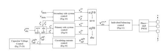
In this section, the control strategy of an AC/AC system based on M³C under asymmetric fault conditions is proposed according to the mathematical model presented in (3)–(7). This strategy allows fully decoupled control of the primary side currents, circulating currents, and secondary side currents. An overview of the proposed control strategy is presented in Figure 7. Firstly, a double αβ0 transformation is applied to the branch currents and voltages. Then, the positive and negative sequences for electrical quantities are separated (as depicted in Figure 8). After that, the control strategies for the primary side system and secondary side system are designed (as shown in Figure 9 and Figure 10). In addition, in order to maintain the stability of capacitor voltages, the capacitor voltage control and the circulating current control are included. Finally, the reference modulation signal is obtained by inverse double αβ0 transformation, and the modulation signal of each submodule is formed by combining the individual balancing control of the submodules within one branch. The trigger pulse is generated by comparing it with the triangular carrier. The following is a detailed analysis of each part of the control strategy.

3.1. Extraction of Positive and Negative Sequence Components

For an asymmetric AC system, negative sequence components exist in both AC voltages and currents. Therefore, it is necessary to separate these components and then extract the positive and negative sequence components, which will be used to design the secondary side controller. In this paper, an asymmetric fault of secondary side system is assumed. The voltages or currents of the system can be expressed as follows:

$$\left[\begin{array}{c}{f}_a\\ f_b\\ f_c\end{array}\right]=\left[\begin{array}{c}{f}^{+}\cos \beta \\ f^{+}\cos \left(\beta -2\pi /3\right)\\ f^{+}\cos \left(\beta +2\pi /3\right)\end{array}\right]+\left[\begin{array}{c}{f}^{-}\cos \gamma \\ f^{-}\cos \left(\gamma +2\pi /3\right)\\ f^{-}\cos \left(\gamma -2\pi /3\right)\end{array}\right]+\left[\begin{array}{c}{f}^0\\ f^0\\ f^0\end{array}\right]$$

(8)

where f_abc denotes voltage or current; $\beta ={\omega }_{1}t+{\alpha }^{+}$ and ω₁ = ω_M where ω_M is the fundamental frequency of the system; $\gamma ={\omega }_{2}t+{\alpha }^{-}$, ω₂ = −ω_M, α⁺ and α⁻ represent the initial phase angles of the positive and negative sequence components respectively, and f⁺ and f⁻ are the amplitude of the positive and negative sequence components, while f⁰ is the zero-sequence component. In this paper, the secondary side system is not grounded, so the zero component is not considered. Equation (8) can be rewritten as follows:

$$\left[\begin{array}{c}{f}_a^{\prime }\\ f_b^{\prime }\\ f_c^{\prime }\end{array}\right]=\left[\begin{array}{c}{f}^{+}\cos \beta \\ f^{+}\cos \left(\beta -2\pi /3\right)\\ f^{+}\cos \left(\beta +2\pi /3\right)\end{array}\right]+\left[\begin{array}{c}{f}^{-}\cos \gamma \\ f^{-}\cos \left(\gamma +2\pi /3\right)\\ f^{-}\cos \left(\gamma -2\pi /3\right)\end{array}\right].$$

(9)

The Park transformation matrices of the positive and negative sequence from the three-phase abc coordinate frames to the two-phase dq rotating coordinate frames are as follows:

$$\{\begin{array}{l}{T}_{abc/dq}^{+}=\frac{2}{3}\left[\begin{array}{ccc}\cos \omega t& \cos \left(\omega t-2\pi /3\right)& \cos \left(\omega t+2\pi /3\right)\\ -\sin \omega t& -\sin \left(\omega t-2\pi /3\right)& -\sin \left(\omega t+2\pi /3\right)\end{array}\right]\\ T_{abc/dq}^{-}=\frac{2}{3}\left[\begin{array}{ccc}\cos \omega t& \cos \left(\omega t+2\pi /3\right)& \cos \left(\omega t-2\pi /3\right)\\ \sin \omega t& \sin \left(\omega t+2\pi /3\right)& \sin \left(\omega t-2\pi /3\right)\end{array}\right].\end{array}$$

(10)

Applying Equations (10) to (9) results in the following sequence separation:

$$\{\begin{array}{l}\left[\begin{array}{c}{f}_d^{{}^{\prime }+}\\ f_q^{{}^{\prime }+}\end{array}\right]=T_{abc/dq}^{+}\left[\begin{array}{c}{f}_a{}^{\prime }\\ f_b{}^{\prime }\\ f_c{}^{\prime }\end{array}\right]=\left[\begin{array}{c}{f}^{+}\cos {\alpha }^{+}\\ f^{+}\sin {\alpha }^{+}\end{array}\right]+\left[\begin{array}{c}{f}^{-}\cos \left(2{\omega }_{1}t+{\alpha }^{-}\right)\\ -f^{-}\sin \left(2{\omega }_{1}t+{\alpha }^{-}\right)\end{array}\right]\\ \left[\begin{array}{c}{f}_d^{{}^{\prime }-}\\ f_q^{{}^{\prime }-}\end{array}\right]=T_{abc/dq}^{-}\left[\begin{array}{c}{f}_a{}^{\prime }\\ f_b{}^{\prime }\\ f_c{}^{\prime }\end{array}\right]=\left[\begin{array}{c}{f}^{-}\cos {\alpha }^{-}\\ f^{-}\sin {\alpha }^{-}\end{array}\right]+\left[\begin{array}{c}{f}^{+}\cos \left(2{\omega }_{2}t+{\alpha }^{+}\right)\\ -f^{+}\sin \left(2{\omega }_{2}t+{\alpha }^{+}\right)\end{array}\right].\end{array}$$

(11)

It can be seen from (11) that after the $T_{abc/dq}^{+}$ transformation, the positive sequence components become the direct current components, while the negative sequence components become the double frequency components. After the $T_{abc/dq}^{-}$ transformation, the negative sequence components become the direct current components, while the positive sequence components become the double frequency components. When these quantities in Equation (11) are delayed by π/2, (12) can be obtained as follows:

$$\left[\begin{array}{c}{f}_d^{{}^{\prime }+}\\ f_q^{{}^{\prime }+}\\ f_d^{{}^{\prime }-}\\ f_q^{{}^{\prime }-}\end{array}\right]e^{-j\frac{\pi }{2}}=\left[\begin{array}{c}{f}^{+}\cos {\alpha }^{+}-f^{-}\cos \left(2{\omega }_{1}t+{\alpha }^{-}\right)\\ f^{+}\sin {\alpha }^{+}+f^{-}\sin \left(2{\omega }_{1}t+{\alpha }^{-}\right)\\ f^{-}\cos {\alpha }^{-}-f^{+}\cos \left(2{\omega }_{2}t+{\alpha }^{+}\right)\\ f^{-}\sin {\alpha }^{-}+f^{+}\sin \left(2{\omega }_{2}t+{\alpha }^{+}\right)\end{array}\right].$$

(12)

Combined with (11) and (12), Equation (13) and the flowchart of Figure 8 can be obtained:

$$\left[\begin{array}{c}{f}_d^{+}\\ f_q^{+}\\ f_d^{-}\\ f_q^{-}\end{array}\right]=\frac{1}{2}\left[\begin{array}{c}{f}_d^{{}^{\prime }+}{+\mathrm{e}}^{-j\frac{\pi }{2}}{f}_d^{{}^{\prime }+}\\ f_q^{{}^{\prime }+}{+\mathrm{e}}^{-j\frac{\pi }{2}}{f}_q^{{}^{\prime }+}\\ f_d^{{}^{\prime }-}{+\mathrm{e}}^{-j\frac{\pi }{2}}{f}_d^{{}^{\prime }-}\\ f_q^{{}^{\prime }-}{+\mathrm{e}}^{-j\frac{\pi }{2}}{f}_q^{{}^{\prime }-}\end{array}\right]$$

(13)

3.2. Control Strategy of the Primary Side System

Figure 1 and Kirchhoff’s current law give $i_{\alpha }^0$, $i_{\beta }^0$, $i_0^{\alpha }$, $i_0^{\beta }$ as follows:

$$\{\begin{array}{l}{i}_{\alpha }^0=\frac{1}{\sqrt{3}}\left(i_{\alpha }^u+i_{\alpha }^v+i_{\alpha }^w\right)=\frac{i_{M\alpha }}{\sqrt{3}}\\ i_{\beta }^0=\frac{1}{\sqrt{3}}\left(i_{\beta }^u+i_{\beta }^v+i_{\beta }^w\right)=\frac{i_{M\beta }}{\sqrt{3}}\\ i_0^{\alpha }=\frac{1}{\sqrt{3}}\left(i_a^{\alpha }+i_b^{\alpha }+i_c^{\alpha }\right)=\frac{i_S^{\alpha }}{\sqrt{3}}\\ i_0^{\beta }=\frac{1}{\sqrt{3}}\left(i_a^{\beta }+i_b^{\beta }+i_c^{\beta }\right)=\frac{i_S^{\beta }}{\sqrt{3}}\end{array}$$

(14)

The equations related to the primary side system can be obtained from Equation (4):

$$\sqrt{3}\left[\begin{array}{c}{v}_S^{\alpha }\\ v_S^{\beta }\end{array}\right]=\frac{1}{\sqrt{3}}L\frac{d}{dt}\left[\begin{array}{c}{i}_S^{\alpha }\\ i_S^{\beta }\end{array}\right]+\left[\begin{array}{c}{v}_0^{\alpha }\\ v_0^{\beta }\end{array}\right].$$

(15)

After applying the dq transformation to Equation (15), the following results can be given as follows:

$$\sqrt{3}\left[\begin{array}{c}{v}_S^d\\ v_S^q\end{array}\right]=\frac{1}{\sqrt{3}}\left[\begin{array}{cc}L\frac{d}{dt}& -{\omega }_{S}L\\ {\omega }_{S}L& L\frac{d}{dt}\end{array}\right]\left[\begin{array}{c}{i}_S^d\\ i_S^q\end{array}\right]+\left[\begin{array}{c}{v}_0^d\\ v_0^q\end{array}\right].$$

(16)

The cross-decoupling control of the primary side system can then be obtained:

$$\left[\begin{array}{c}{v}_0^{d\ast }\\ v_0^{q\ast }\end{array}\right]=\sqrt{3}\left[\begin{array}{c}{v}_S^d\\ v_S^q\end{array}\right]-\frac{{\omega }_{S}L}{\sqrt{3}}\left[\begin{array}{cc}0& -1\\ 1& 0\end{array}\right]\left[\begin{array}{c}{i}_S^d\\ i_S^q\end{array}\right]-K_S\left(1+\frac{1}{s{T}_s}\right)\left(\left[\begin{array}{c}{i}_S^{d\ast }\\ i_S^{q\ast }\end{array}\right]-\left[\begin{array}{c}{i}_S^d\\ i_S^q\end{array}\right]\right)$$

(17)

where K_S and T_S represent the proportion and time constants, respectively, and $i_s^{dq*}$ means the reference value of the system current on the dq reference frames. Additionally, in order to achieve a unity power factor operation, the reactive current is set to 0, and the active current is controlled by the outer power loop control and the overall capacitor voltage control:

$$i_S^{d\ast }=\frac{p^{\ast }}{v_S^d}+K_A\left(1+\frac{1}{s{T}_A}\right)\left(V_C^{\ast }-\overline{V_C}\right)$$

(18)

where K_A and T_A represent the proportion and time constant, respectively, and $p^{\ast }$, $V_C^{\ast }$, and $\overline{V_C}$ represent the active power setting value, the rated capacitor voltage, and the average voltage of all submodule capacitors, respectively.

In summary, the control block diagram of the primary side system can be obtained as shown in Figure 9.

3.3. Control Strategy of the Secondary Side System

Combining Equations (5) and (14), the corresponding equations for the secondary side system are as follows:

$$-\sqrt{3}\left[\begin{array}{c}{v}_M^{\alpha }\\ v_M^{\beta }\end{array}\right]=\frac{1}{\sqrt{3}}L\frac{d}{dt}\left[\begin{array}{c}{i}_M^{\alpha }\\ i_M^{\beta }\end{array}\right]+\left[\begin{array}{c}{v}_{\alpha }^0\\ v_{\beta }^0\end{array}\right].$$

(19)

Similarly, when the dq transformation is applied, we get

$$-\sqrt{3}\left[\begin{array}{c}{v}_M^d\\ v_M^q\end{array}\right]=\frac{1}{\sqrt{3}}\left[\begin{array}{cc}L\frac{d}{dt}& -{\omega }_{M}L\\ {\omega }_{M}L& L\frac{d}{dt}\end{array}\right]\left[\begin{array}{c}{i}_M^d\\ i_M^q\end{array}\right]+\left[\begin{array}{c}{v}_d^0\\ v_q^0\end{array}\right].$$

(20)

Because the voltages and currents should be separated into positive and negative sequences under asymmetric fault conditions, the decoupled controllers for the positive and negative sequences can be designed separately according to the following equations:

$$\left[\begin{array}{c}{v}_{d+}^{0\ast }\\ v_{q+}^{0\ast }\end{array}\right]=-\sqrt{3}\left[\begin{array}{c}{v}_M^{d+}\\ v_M^{q+}\end{array}\right]-\frac{{\omega }_{M}L}{\sqrt{3}}\left[\begin{array}{cc}0& -1\\ 1& 0\end{array}\right]\left[\begin{array}{c}{i}_M^{d+}\\ i_M^{q+}\end{array}\right]-K_{M1}\left(1+\frac{1}{s{T}_{M1}}\right)\left(\left[\begin{array}{c}{i}_M^{d+\ast }\\ i_M^{q+\ast }\end{array}\right]-\left[\begin{array}{c}{i}_M^{d+}\\ i_M^{q+}\end{array}\right]\right)$$

(21)

$$\left[\begin{array}{c}{v}_{d-}^{0\ast }\\ v_{q-}^{0\ast }\end{array}\right]=-\sqrt{3}\left[\begin{array}{c}{v}_M^{d-}\\ v_M^{q-}\end{array}\right]-\frac{{\omega }_{M}L}{\sqrt{3}}\left[\begin{array}{cc}0& 1\\ -1& 0\end{array}\right]\left[\begin{array}{c}{i}_M^{d-}\\ i_M^{q-}\end{array}\right]-K_{M2}\left(1+\frac{1}{s{T}_{M2}}\right)\left(\left[\begin{array}{c}{i}_M^{d-\ast }\\ i_M^{q-\ast }\end{array}\right]-\left[\begin{array}{c}{i}_M^{d-}\\ i_M^{q-}\end{array}\right]\right)$$

(22)

where K_M1, K_M2 and T_M1, T_M2 represent the proportion and time constants, respectively, and d⁺, d⁻, q⁺, and q⁻ denote the positive and negative sequence of electrical quantities (voltages or currents) on the dq reference frames.

In the above section, the controllers based on positive and negative sequences are introduced for an asymmetric ac system. The advantage of this method is that it is easy to understand because the positive and negative sequence controllers are similar to those of the symmetric AC system. Thus, the design methods can be analogized. The disadvantage is that the control system and its implementation are complex and can also produce errors and delays that cannot be ignored in the control loop, while the proportional resonant controller (PR) can be used to regulate positive and negative sequence currents at the same time. Moreover, compared to design methods based on positive and negative sequence controllers separately, only two PR controllers are needed instead of four for the dq-based controllers. In a word, the proportional resonant controller is preferable to regulate the fault currents of a secondary side system, which consists of both positive and negative sequences simultaneously. Therefore, considering Equation (5), the voltage references to achieve the decoupled current control of the secondary side system using PR controllers should be given as follows:

$$\left[\begin{array}{c}{v}_{\alpha }^{0*}\\ v_{\beta }^{0*}\end{array}\right]=\left[\begin{array}{c}{v}_{\alpha \_ref}\\ v_{\beta \_ref}\end{array}\right]-L\frac{d}{dt}\left[\begin{array}{c}{i}_{M\alpha }\\ i_{M\beta }\end{array}\right]-C_{PR}(s)\left(\left[\begin{array}{c}{i}_{\alpha \_ref}\\ i_{\beta \_ref}\end{array}\right]-\left[\begin{array}{c}{i}_{M\alpha }\\ i_{M\beta }\end{array}\right]\right)$$

(23)

where $C_{PR}=K_p+K_i\frac{s}{s^2+{\omega }^2}$ represents the transfer function of the proportional resonant controller, and K_p and K_i denote the proportion and resonant coefficients, respectively.

In summary, the control block diagram of the secondary side system is as follows:

3.4. Power Control

According to the theory of instantaneous reactive power [22], the instantaneous active power and reactive power of the secondary side system can be expressed as:

$$\{\begin{array}{l}P=P_1+P_{s2}\sin \left(2\omega t\right)+P_{c2}\cos \left(2\omega t\right)\\ Q=Q_1+Q_{s2}\sin \left(2\omega t\right)+Q_{c2}\cos \left(2\omega t\right)\end{array}$$

(24)

where P₁ and Q₁ are the DC components of active power and reactive power, respectively, and P_s2 and P_c2 represent the double frequency oscillations in active power, while Q_s2 and Q_c2 are those of the reactive power. As taken from [23,24], the relation between the currents, the power, and the voltages in the αβ reference frames are

$$\{\begin{array}{l}{P}_1=\frac{3}{2}\left(v_{\alpha }^{0+}{i}_{\alpha }^{+}+v_{\beta }^{0+}{i}_{\beta }^{+}+v_{\alpha }^{0-}{i}_{\alpha }^{-}+v_{\beta }^{0-}{i}_{\beta }^{-}\right)\\ P_{s2}=\frac{3}{2}\left(v_{\beta }^{0-}{i}_{\alpha }^{+}-v_{\alpha }^{0-}{i}_{\beta }^{+}-v_{\beta }^{0+}{i}_{\alpha }^{-}+v_{\alpha }^{0+}{i}_{\beta }^{-}\right)\\ P_{c2}=\frac{3}{2}\left(v_{\alpha }^{0+}{i}_{\alpha }^{-}+v_{\beta }^{0+}{i}_{\beta }^{-}+v_{\alpha }^{0-}{i}_{\alpha }^{+}+v_{\beta }^{0-}{i}_{\beta }^{+}\right)\\ Q_1=\frac{3}{2}\left(v_{\beta }^{0+}{i}_{\alpha }^{+}-v_{\alpha }^{0+}{i}_{\beta }^{+}+v_{\beta }^{0-}{i}_{\alpha }^{-}-v_{\alpha }^{0-}{i}_{\beta }^{-}\right)\\ Q_{s2}=\frac{3}{2}\left(v_{\alpha }^{0+}{i}_{\alpha }^{-}+v_{\beta }^{0+}{i}_{\beta }^{-}-v_{\alpha }^{0-}{i}_{\alpha }^{+}-v_{\beta }^{0-}{i}_{\beta }^{+}\right)\\ Q_{c2}=\frac{3}{2}\left(v_{\beta }^{0+}{i}_{\alpha }^{-}-v_{\alpha }^{0+}{i}_{\beta }^{-}+v_{\beta }^{0-}{i}_{\alpha }^{+}-v_{\alpha }^{0-}{i}_{\beta }^{+}\right)\end{array}$$

(25)

It is important to note that there are four degrees of freedom ( $i_{\alpha }^{+}$, $i_{\beta }^{+}$, $i_{\alpha }^{-}$, $i_{\beta }^{-}$) to control six variables (P₁, Q₁, P_s2, P_c2, Q_s2, Q_c2). Thus, it is necessary to choose variables according to the control objectives. In this paper, P₁, Q₁, P_s2, and P_c2 are selected as control variables. Therefore, it can be concluded that

$$\left[\begin{array}{c}{i}_{\alpha }^{+}\\ i_{\beta }^{+}\\ i_{\alpha }^{-}\\ i_{\beta }^{-}\end{array}\right]={\left[\begin{array}{cccc}{v}_{\alpha }^{0+}& v_{\beta }^{0+}& v_{\alpha }^{0-}& v_{\beta }^{0-}\\ v_{\beta }^{0+}& -v_{\alpha }^{0+}& v_{\beta }^{0-}& -v_{\alpha }^{0-}\\ v_{\beta }^{0-}& -v_{\alpha }^{0-}& -v_{\beta }^{0+}& v_{\alpha }^{0+}\\ v_{\alpha }^{0-}& v_{\beta }^{0-}& v_{\alpha }^{0+}& v_{\beta }^{0+}\end{array}\right]}^{-1}\left[\begin{array}{c}\frac{2}{3}{P}_1\\ \frac{2}{3}{Q}_1\\ \frac{2}{3}{P}_{s2}\\ \frac{2}{3}{P}_{c2}\end{array}\right].$$

(26)

3.5. Capacitor Voltage Control

Capacitor voltage control consists of the capacitor voltage control for DC components and the capacitor voltage control for AC components. The capacitor voltage control for DC component is called a “DC capacitor voltage balancing control” [25,26], which regulates the DC components of all the capacitor voltages to be balanced. The capacitor voltage control for AC components is referred to as a “fluctuation mitigating control” [27,28], which mitigates the amplitude of AC voltage fluctuation. These controls are all realized by adjusting the four circulating currents appropriately.

On the whole, capacitor voltage control mainly consists of the following three subcontrols:

1) Overall voltage control: This control adjusts the algebraic average value of all capacitor voltages to the rated value. A subcontrol has been implemented in the primary side system control strategy, as shown in Figure 9.

2) Branch balancing control: This control balances the voltage of the algebraic average values of the DC capacitor voltage among the nine branches, including the branches of the voltage balancing control between the three subconverters, which is referred to as the “inter-subconverter balancing control” and the three branch voltage balancing within one subconverter, which is referred to as an “inner-subconverter balancing control” [19,20,21]. These controls are mainly realized by adjusting four circulating currents $i_{\alpha \beta }^{\alpha \beta \ast }$. The methods presented in [21] will be adopted in this paper and will not be discussed in detail here.

a) Inter-subconverter balancing control: The commands for the four circulating currents are as follows:

$$\left[\begin{array}{cc}{i}_{\alpha }^{\alpha \ast }& i_{\alpha }^{\beta \ast }\\ i_{\beta }^{\alpha \ast }& i_{\beta }^{\beta \ast }\end{array}\right]=K_{0i}\left(\left[\begin{array}{cc}-{\overline{v}}_{C\alpha }^0\sin {\theta }_s& {\overline{v}}_{C\alpha }^0\cos {\theta }_s\\ -{\overline{v}}_{C\beta }^0\sin {\theta }_s& {\overline{v}}_{C\beta }^0\cos {\theta }_s\end{array}\right]+\left[\begin{array}{cc}{\overline{v}}_{C0}^{\alpha }\sin {\theta }_M& {\overline{v}}_{C0}^{\beta }sin{\theta }_M\\ -{\overline{v}}_{C0}^{\alpha }\cos {\theta }_M& -{\overline{v}}_{C0}^{\beta }\cos {\theta }_M\end{array}\right]\right)$$

(27)

b) Inner-subconverter balancing control: The commands for the four circulating currents are as follows:

$$\left[\begin{array}{cc}{i}_{\alpha }^{\alpha \ast }& i_{\alpha }^{\beta \ast }\\ i_{\beta }^{\alpha \ast }& i_{\beta }^{\beta \ast }\end{array}\right]=-K_1\left(\left[\begin{array}{cc}{\overline{v}}_{C\alpha }^{\alpha }\sin {\theta }_s& {\overline{v}}_{C\alpha }^{\alpha }\cos {\theta }_s\\ {\overline{v}}_{C\beta }^{\alpha }\sin {\theta }_s& {\overline{v}}_{C\beta }^{\alpha }\cos {\theta }_s\end{array}\right]+\left[\begin{array}{cc}{\overline{v}}_{C\alpha }^{\beta }\cos {\theta }_s& -{\overline{v}}_{C\alpha }^{\beta }\sin {\theta }_s\\ {\overline{v}}_{C\beta }^{\beta }\cos {\theta }_s& -{\overline{v}}_{C\beta }^{\beta }\cos {\theta }_s\end{array}\right]\right)$$

(28)

where θ_s and θ_M are the voltage phase of both side systems, and K_0i and K₁ are the proportional control coefficients. Here, ${\overline{v}}_{C\alpha \beta }^0$, ${\overline{v}}_{C0}^{\alpha \beta }$, ${\overline{v}}_{C\alpha \beta }^{\alpha \beta }$ represent the algebraic average value of the branch voltages after the double αβ0 transformation.

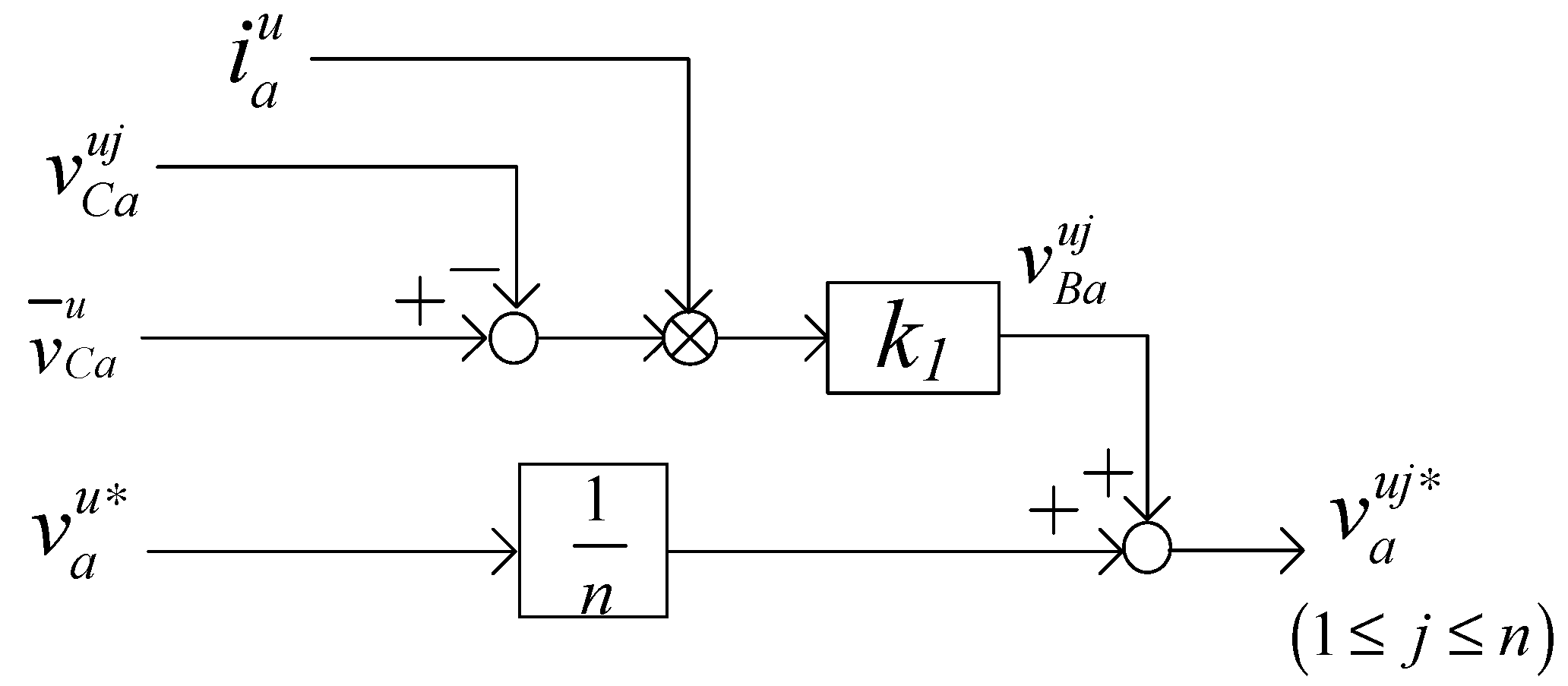
3) Individual balancing control: This control is used to achieve voltage balancing among n submodules within a single branch. When voltage imbalance occurs within a branch, individual balancing control plays a role in eliminating the voltage imbalance. As shown in Figure 11, taking branch-au of subconverter a as an example. In the figure, ${\overline{v}}_{Ca}^u$, $v_a^{u\ast }$, and $v_{Ca}^{uj}$ denote the algebraic average value of the capacitor voltages and the modulated signal in branch-au and the capacitor voltage of the j-th submodule in branch-au, respectively. k₁ represents the proportional coefficient. Like other modular multilevel cascade converters, by adding a voltage increment that depends on the direction of the branch current to the modulation signal, a positive or negative power that charges or discharges the capacitor will be formed balance capacitor voltage within the branch. $v_a^{uj\ast }$(1 < j < n) represents the voltage references of n submodules. These references will be used to generate trigger pulses by comparing them with triangular carriers.

3.6. Circulating Current Control

Basically, these circulating currents should be regulated to zero to reduce power loss because they make no contribution to transferring active power between both systems. However, as mentioned earlier, voltage balancing between the nine branches and a mitigation of the AC voltage fluctuation can be achieved by properly adjusting the four circulating currents.

From Equation (6), the equation for the four circulating currents is as follows:

$$\left[\begin{array}{cc}0& 0\\ 0& 0\end{array}\right]=L\frac{d}{dt}\left[\begin{array}{cc}{i}_{\alpha }^{\alpha }& i_{\alpha }^{\beta }\\ i_{\beta }^{\alpha }& i_{\beta }^{\beta }\end{array}\right]+\left[\begin{array}{cc}{v}_{\alpha }^{\alpha }& v_{\alpha }^{\beta }\\ v_{\beta }^{\alpha }& v_{\beta }^{\beta }\end{array}\right].$$

(29)

Thus, the voltage commands to achieve decoupled control for circulating currents can be given as follows:

$$\left[\begin{array}{cc}{v}_{\alpha }^{\alpha \ast }& v_{\alpha }^{\beta \ast }\\ v_{\beta }^{\alpha \ast }& v_{\beta }^{\beta \ast }\end{array}\right]=-k_2\left(\left[\begin{array}{cc}{i}_{\alpha }^{\alpha \ast }& i_{\alpha }^{\beta \ast }\\ i_{\beta }^{\alpha \ast }& i_{\beta }^{\beta \ast }\end{array}\right]-\left[\begin{array}{cc}{i}_{\alpha }^{\alpha }& i_{\alpha }^{\beta }\\ i_{\beta }^{\alpha }& i_{\beta }^{\beta }\end{array}\right]\right)$$

(30)

where k₂ represents the proportional constant and $i_{\alpha \beta }^{\alpha \beta \ast }$ means the reference values of the four circulating currents, which are given by the capacitor voltage control in Section 3.5.

4. Assessment in Simulated Experiments

To verify the effectiveness of the proposed control strategy under asymmetric fault conditions, a simulation system, as shown in Figure 1, was built in the PSCAD/EMTDC software. Both system parameters are described in

Table A2. List of the simulation system parameters.

Parameter Description	Symbol	Value
Primary side system voltage	V1(L-L)	10 kV
Secondary side system voltage	V2(L-L)	10 kV
Rated voltage of capacitor	Vc *	1.5 kV
Number of submodules within each branch	n	20
Capacitance value	C	8400 μF
System frequency	f1	50 Hz
System frequency	f2	50 Hz
Switching frequency	fsw	2 kHz
Branch inductor	L	2.4 mH
Constant	Kp	20
Constant	Ki	1000
Constant	Ks	10
Constant	Ts	0.001
Constant	KA	10
Constant	TA	0.1
Constant	k1	0.1
Constant	k2	1.5

. The system line-to-line voltages on both sides are 10 kV, the number of submodules within each branch is n = 20 (taking redundancy into account), the rated capacitor voltage u_cN is 1.5 kV, the system frequencies on both sides are 50 Hz, and the carrier phase-shifted PWM is adopted when the switching frequency f_s is 2 kHz. The changes in the active power command of both systems are shown in

Table 1. The set values of both systems’ active power.

Time (s)	P1 (MW)	P2 (MW)
0~1 s	7.5	−7.5
1 s~1.5 s	3.5	−3.5
1.5 s~2 s	7.5	−7.5

, while the reactive power command of Q₁ = Q₂ = 0 ensures operation of the unity power factor. In the simulation case, at t = 1 s, a BC-phase short-circuit fault occurs, and the fault lasts for 0.5 s.

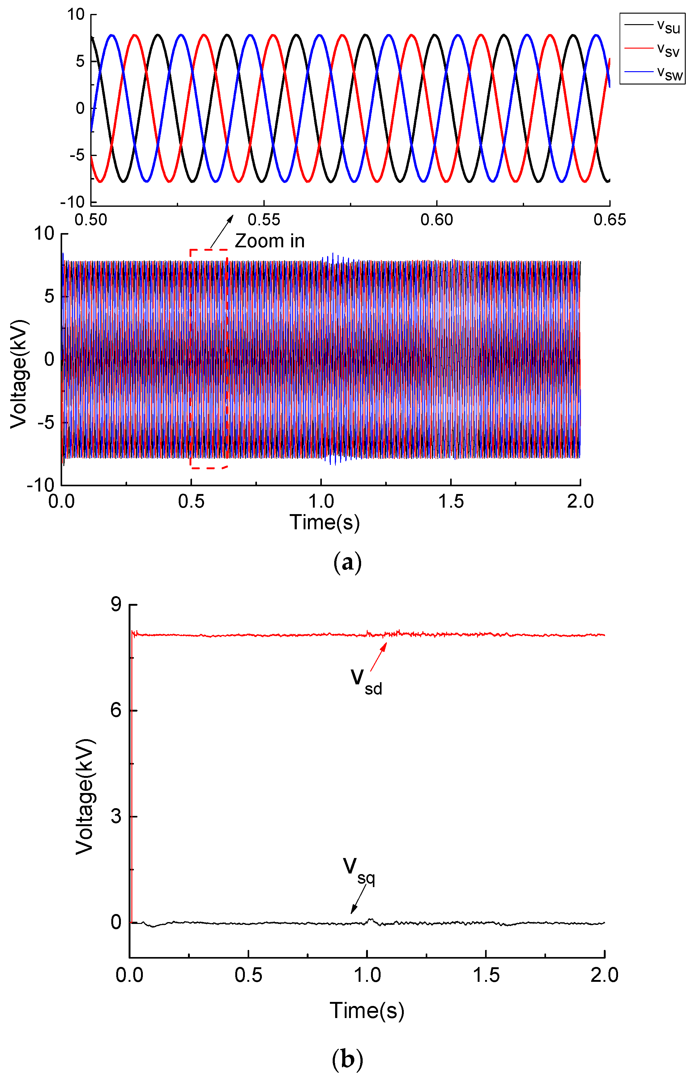
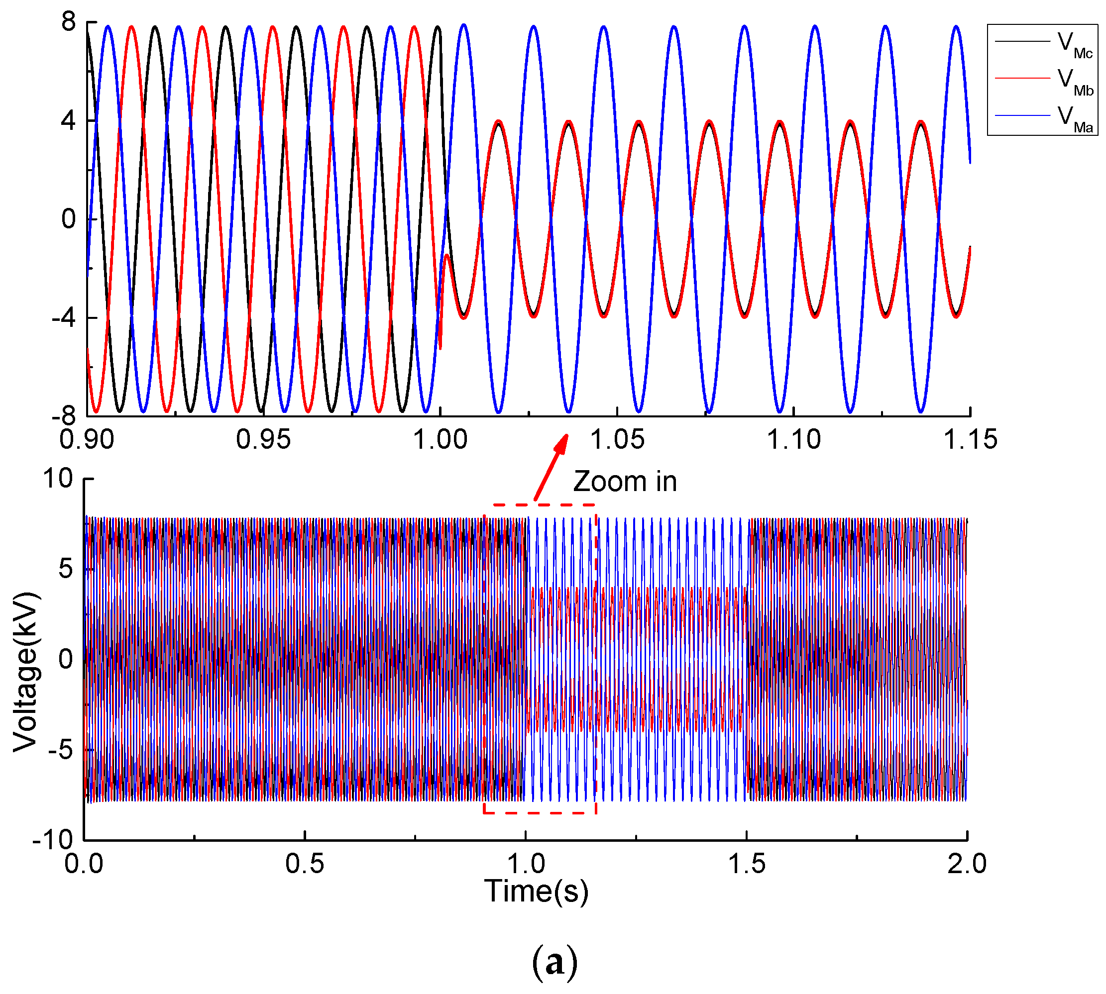
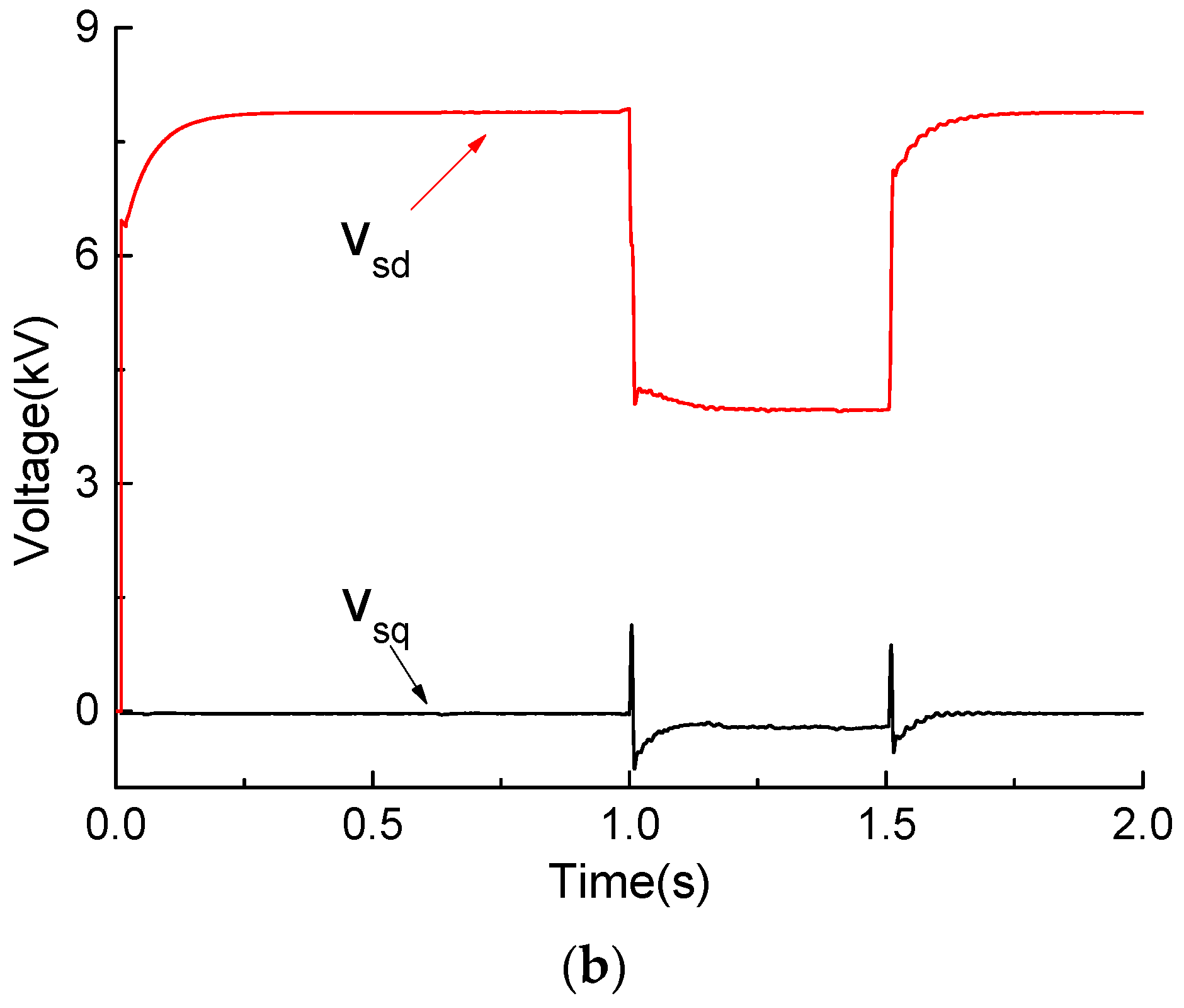
Figure 12 and Figure 13 show the three-phase voltages for both systems and their d-q waveforms. It can be seen that the voltages of the primary side system maintain their rated values in both normal and fault conditions and are not greatly affected (as shown in Figure 12a), while the voltages of the BC-phase in the secondary side system decrease when the fault occurs, as shown in Figure 13a.

The active power P₁ of the primary side and the active power P₂ of the secondary side system can be seen in Figure 14, which clearly shows that the active power can quickly track its set values. Furthermore, the whole system can still maintain stable operation and transmit a certain amount of active power during the fault period. Additionally, there are no double-frequency oscillations in the active/reactive power of the primary side system, but double-frequency oscillations do appear in the secondary side system during the fault, as shown in Figure 14.

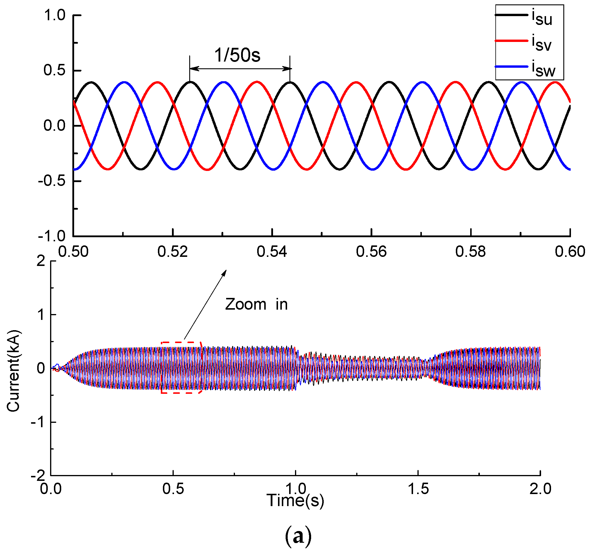
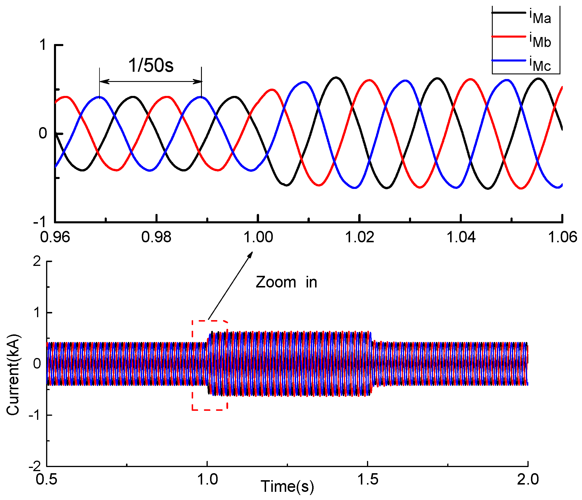
As depicted in Figure 15 and Figure 16, the frequencies of both systems are 50 Hz, and when the fault appears, the currents of the primary side system decrease due to the system’s decreased active power, while the currents of the secondary side system increase (as shown in Figure 16). When the fault is cleared, the system currents on both sides are restored to the initial value, with a change in the active power.

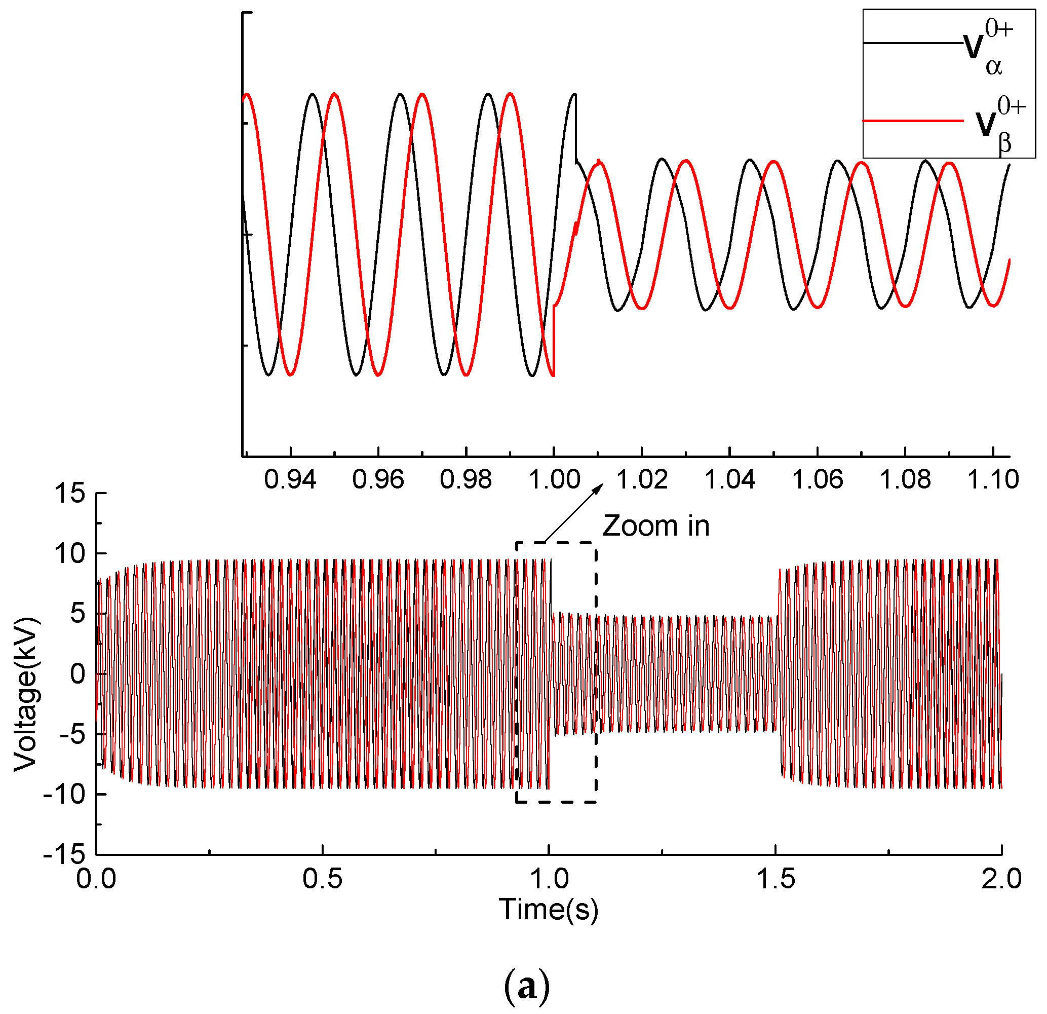
Figure 17 shows the positive and negative sequence components of the secondary side system voltage in αβ reference frames. As depicted in Figure 17b, as soon as the fault is applied, the negative sequence voltage components appear at t =1 s and disappear rapidly with the removal of the asymmetric fault at t = 1.5 s.

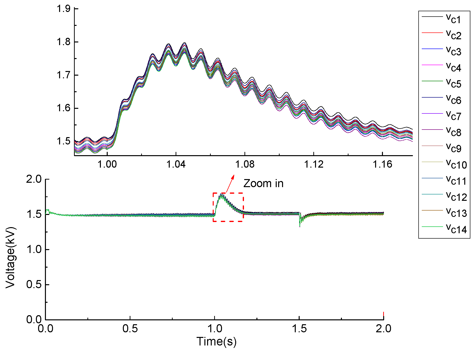
The branch module voltage is multilevel, which can be seen in Figure 18, and its amplitude decreases slightly during the fault. The capacitor voltages are illustrated in Figure 19. When the fault appears, a slight increase can be observed. The capacitor voltages are balanced, and their fluctuations are within an acceptable level.

In summary, all the above waveforms show that the system can still operate stably in the case of an AC asymmetric fault, thereby confirming the effectiveness of the proposed control strategy.

5. Conclusions

This paper has proposed an asymmetric fault control strategy for an AC/AC system based on a modular multilevel matrix converter (M³C) with focus on the short-circuit fault of the BC-phase in the secondary side system. The working principle of the M³C is introduced by theoretical analysis and simulation verification. In the case of an asymmetric fault condition, the positive and negative sequence components of the voltages and currents are separated, and then the proportional resonant controller is used to realize decoupled control in the αβ reference frames. Finally, the proposed control strategy is confirmed by simulation in PSCAD/EMTDC software. The simulation results show that the whole system can still maintain stable operation and transmit a certain amount of active power, according to the set values during the period of fault. Furthermore, the capacitor voltages are balanced, with a slight increase during the fault period. In the future, experiments will be carried out to further verify the advantages and effectiveness of this control strategy.

References

- Marqurdt, R. Stromrichterschaltungen Mit Verteilten Energies-Peichern. German Patent DE10103031A1, 24 January 2001. [Google Scholar]
- Oates, C. A methodology for developing ‘Chainlink’ converters. In Proceedings of the 13th Europe Conference on Power Electronics and Applications, Barcelona, Spain, 8–10 September 2009. [Google Scholar]
- Karwatzki, D.; Von-Hofen, M.; Baruschka, L.; Mertens, A. Operation of modular multilevel matrix converters with failed branches. In Proceedings of the 40th Annual Conference of the IEEE Industrial Electronics Society, Dallas, TX, USA, 29 October–1 November 2014. [Google Scholar]
- Meng, Y.; Wang, J.; Li, L. Mathematical mod-el and control strategy of M3C converter based on double dq coordinate transformation. J. Electr. Eng. China 2016, 36, 4702–4712. [Google Scholar]
- Angkititrakul, S.; Erickson, R.W. Control and implementation of a new modular matrix converter. In Proceedings of the Nineteenth Annual IEEE Applied Power Electronics Conference and Exposition, Anaheim, CA, USA, 22–26 February 2004. [Google Scholar]
- Angkititrakul, S.; Erickson, R.W. Capacitor voltage balancing control for a modular matrix converter. In Proceedings of the Twenty-First Annual IEEE Applied Power Electronics Conference and Exposition, Dallas, TX, USA, 19–23 March 2006. [Google Scholar]
- Mora, A.; Espinoza, M.; Díaz, M.; Cárdenas, R. Model Predictive Control of Modular Multilevel Matrix Converter. In Proceedings of the 24th IEEE International Symposium on Industrial Electronics (ISIE), Buzios, Brazil, 3–5 June 2015. [Google Scholar]
- Fan, B.; Wang, K.; Wheeler, P. An Optimal Full Frequency Control Strategy for the Modular Multilevel Matrix Converter Based on Predictive Control. IEEE Trans. Power Electron. 2018, 33, 6608–6621. [Google Scholar] [CrossRef]
- Kammerer, F.; Kolb, J.; Braun, M. A novel cascaded vector control scheme for the Modular Multilevel Matrix Converter. In Proceedings of the 37th Annual Conference of the IEEE Industrial Electronics Society, Melbourne, Australia, 7–10 November 2011. [Google Scholar]
- Kammerer, F.; Kolb, J.; Braun, M. Fully decoupled current control and energy balancing of the Modular Multilevel Matrix Converter. In Proceedings of the 15th International Power Electronics and Motion Control Conference (EPE/PEMC), Novi Sad, Serbia, 4–6 September 2012. [Google Scholar]
- Kammerer, F.; Gommeringer, M.; Kolb, J.; Braun, M. Energy balancing of the Modular Multilevel Matrix Converter based on a new transformed arm power analysis. In Proceedings of the 16th European Conference on Power Electronics and Applications, Lappeenranta, Finland, 26–28 August 2014. [Google Scholar]
- Li, F.; Wang, G. Steady-state analysis of capacitor voltage ripple in modular multilevel matrix converter. Chin. J. Electr. Eng. 2013, 33, 52–58. [Google Scholar]
- Li, F.; Wang, G.; Liu, R. Control method for expanding low frequency operation range of modular multilevel matrix converter. Power Syst. Autom. 2016, 40, 132–138. [Google Scholar]
- Li, F.; Wang, G. Control strategy for low-frequency operation of modular multilevel matrix converters with similar input and output frequencies. J. Electr. Technol. 2016, 31, 107–114. [Google Scholar]
- Miura, Y.; Mizutani, T.; Ito, M.; Ise, T. Modular multilevel matrix converter for low frequency AC transmission. In Proceedings of the 10th IEEE International Conference on Power Electronics and Drive Systems (PEDS), Kitakyushu, Japan, 22–25 April 2013. [Google Scholar]
- Huang, L.; Yang, X.; Zhang, B.; Qiao, L. Hierarchical model predictive control of modular multilevel matrix converter for low frequency AC transmission. In Proceedings of the 9th International Conference on Power Electronics and ECCE Asia (ICPE-ECCE Asia), Seoul, Korea, 1–5 June 2015. [Google Scholar]
- Ma, J.; Dahidah, M.; Pickert, V. Modular multilevel matrix converter for offshore low frequency AC transmission system. In Proceedings of the 26th IEEE International Symposium on Industrial Electronics (ISIE), Edinburgh, UK, 19–21 June 2017. [Google Scholar]
- Liu, S.; Wang, X.; Meng, Y.; Sun, P. A Decoupled Control Strategy of Modular Multilevel Matrix Converter for Fractional Frequency Transmission System. IEEE Trans. Power Deliv. 2017, 32, 2111–2121. [Google Scholar] [CrossRef]
- Kawamura, W.; Hagiwara, M.; Akagi, H. Control and experiment of a 380-V, 15-kW motor drive using modular multilevel cascade converter based on triple-star bridge cells (MMCC-TSBC). In Proceedings of the International Power Electronics Conference (IPEC-Hiroshima 2014—ECCE ASIA), Hiroshima, Japan, 18–21 May 2014. [Google Scholar]
- Kawamura, W.; Akagi, H. Control of the modular multilevel cascade converter based on triple-star bridge-cells (MMCC-TSBC) for motor drives. In Proceedings of the 2012 IEEE Energy Conversion Congress and Exposition (ECCE), Raleigh, NC, USA, 15–20 September 2012. [Google Scholar]
- Kawamura, W.; Hagiwara, M.; Akagi, H. Control and Experiment of a Modular Multilevel Cascade Converter Based on Triple-Star Bridge Cells. IEEE Trans. Ind. Appl. 2014, 50, 3536–3548. [Google Scholar] [CrossRef]
- Hong-Seok, S.; Kwanghee, N. Dual current control scheme for PWM converter under unbalanced input voltage conditions. IEEE Trans. Ind. Electron. 1999, 46, 953–959. [Google Scholar] [CrossRef]
- Cárdenas, R.; Díaz, M.; Rojas, F.; Clare, J. Resonant control system for low-voltage ride-through in wind energy conversion systems. IET Power Electron. 2016, 9, 1297–1305. [Google Scholar] [CrossRef]
- Díaz, M.; Cárdenas, R. Analysis of synchronous and stationary reference frame control strategies to fulfill LVRT requirements in Wind Energy Conversion Systems. In Proceedings of the Ninth International Conference on Ecological Vehicles and Renewable Energies (EVER), Monte-Carlo, Monaco, 25–27 March 2014. [Google Scholar]
- Kawamura, W.; Hagiwara, M.; Akagi, H. A broad range of frequency control for the modular multilevel cascade converter based on triple-star bridge-cells (MMCC-TSBC). In Proceedings of the IEEE Energy Conversion Congress and Exposition, Denver, CO, USA, 15–19 September 2013. [Google Scholar]
- Kawamura, W.; Hagiwara, M.; Akagi, H. Experimental verification of a modular multilevel cascade converter based on triple-star bridge-cells (MMCC-TSBC) for motor drives. In Proceedings of the 1st International Future Energy Electronics Conference (IFEEC), Tainan, Taiwan, 3–6 November 2013. [Google Scholar]
- Kawamura, W.; Chiba, Y.; Hagiwara, M.; Akagi, H. Experimental verification of TSBC-based electrical drives when the motor frequency is passing through, or equal to, the supply frequency. In Proceedings of the IEEE Energy Conversion Congress and Exposition (ECCE), Montreal, QC, Canada, 20–24 September 2015. [Google Scholar]
- Kawamura, Y.; Chiba, M.; Akagi, H. Experimental Verification of an Electrical Drive Fed by a Modular Multilevel TSBC Converter When the Motor Frequency Gets Closer or Equal to the Supply Frequency. IEEE Trans. Ind. Appl. 2017, 53, 2297–2306. [Google Scholar] [CrossRef]
Figure 1.
The topology of modular multilevel matrix converter (M3C).
Figure 2.
System voltage waveforms.
Figure 3.
Secondary side system current waveforms.
Figure 4.
Module voltage waveform of branch-au.
Figure 5.
Branch current waveforms of subconverter a and b: (a) subconverter a; (b) subconverter b.
Figure 6.
Capacitor voltages.
Figure 7.
Overview of the control strategy.
Figure 8.
Positive and negative sequence separation and extraction flow chart.
Figure 9.
Control block diagram of the primary side system.
Figure 10.
Control block diagram of the secondary side system.
Figure 11.
Block diagram of the individual capacitor voltage balancing of branch-au.
Figure 12.
Primary side system voltage curves: (a) system voltages; (b) d–q waveforms.
Figure 13.
Secondary side system voltage curves: (a) system voltages; (b) d–q waveforms.
Figure 14.
Power curves of both side systems.
Figure 15.
Current waveforms of the primary side system: (a) system currents; (b) d–q waveforms.
Figure 16.
Current waveforms of the secondary side system.
Figure 17.
Positive and negative sequence components of the secondary side system voltage in the αβ reference frames: (a) positive sequence voltages; (b) negative sequence voltages.
Figure 18.
Figure 19.
Capacitor voltage waveforms.