Large Eddy Simulation of an Onshore Wind Farm with the Actuator Line Model Including Wind Turbine’s Control below and above Rated Wind Speed


IMFIA, Facultad de Ingeniería, Universidad de la República, 11200 Montevideo, Uruguay
*
Author to whom correspondence should be addressed.
Energies 2019, 12(18), 3508; https://doi.org/10.3390/en12183508
Submission received: 23 July 2019
/
Revised: 27 August 2019
/
Accepted: 29 August 2019
/
Published: 11 September 2019
(This article belongs to the Special Issue Recent Advances in Aerodynamics of Wind Turbines)
Abstract
:As the size of wind turbines increases and their hub heights become higher, which partially explains the vertiginous increase of wind power worldwide in the last decade, the interaction of wind turbines with the atmospheric boundary layer (ABL) and between each other is becoming more complex. There are different approaches to model and compute the aerodynamic loads, and hence the power production, on wind turbines subject to ABL inflow conditions ranging from the classical Blade Element Momentum (BEM) method to Computational Fluid Dynamic (CFD) approaches. Also, modern multi-MW wind turbines have a torque controller and a collective pitch controller to manage power output, particularly in maximizing power production or when it is required to down-regulate their production. In this work the results of a validated numerical method, based on a Large Eddy Simulation-Actuator Line Model framework, was applied to simulate a real 7.7 MNW onshore wind farm on Uruguay under different wind conditions, and hence operational situations are shown with the aim to assess the capability of this approach to model actual wind farm dynamics. A description of the implementation of these controllers in the CFD solver Caffa3d, presenting the methodology applied to obtain the controller parameters, is included. For validation, the simulation results were compared with 1 Hz data obtained from the Supervisory Control and Data Acquisition System of the wind farm, focusing on the temporal evolution of the following variables: Wind velocity, rotor angular speed, pitch angle, and electric power. In addition to this, simulations applying active power control at the wind turbine level are presented under different de-rate signals, both constant and time-varying, and were subject to different wind speed profiles and wind directions where there was interaction between wind turbines and their wakes.
1. Introduction
Wind energy has expanded worldwide in the last decade. The installed capacity of wind power has increased close to 10% in 2017 [1], multiplying by almost 4.5 times between 2008 and 2017. Wind energy has become one of the main energy sources in some countries, achieving penetration levels in power generation of more than 30% in countries like Denmark [2] and Uruguay [3]. This development has been possible because of technological improvements making wind turbines more efficient, larger in size (rotor diameter, hub height, and rated power), and more capable of contributing to the electric grid regulation by supplying ancillary services [4,5,6]. In [4], the authors analyzed the evolution of onshore wind turbines installed worldwide between 2005 and 2014, finding that the rotor diameter increased on average around 42.3% in that period with a clear trend towards longer blades. In the same way, the wind turbine’s rated power has increased in that period, from 1.38 MW in 2005 to 2.20 MW in 2014 (59%). A similar trend can be observed when looking at the evolution of hub height. In [5], an international survey is presented where 163 of the world’s foremost wind experts were asked to predict, among other things, the reduction of the levelized cost of energy (LCOE), the main drivers in its reduction, and the turbine size. Regarding the latter, the median of expert responses for typical rotor diameter (hub height) in 2030 was 135 m (115 m) and 190 m (125 m) for onshore wind turbines and fixed-bottom offshore wind turbines, respectively. The trend towards longer blades and higher hub heights will probably continue in the following years, so wind turbine rotors will sweep a larger portion of the atmospheric boundary layer (ABL). In addition to this, longer blades mean that blade deformation and aeroelasticity will play a major role in the near future. From the above, the interaction of wind turbines with the ABL and between each other will become more complex.
There are different approaches to modeling and computing aerodynamic loads, and hence the power production, on wind turbines subject to ABL inflow conditions. The aerodynamic models range from the classical Blade Element Momentum (BEM) method to Computational Fluid Dynamic (CFD) approaches [7,8,9,10]. The former is still the most widely-used model in aeroelastic codes, both within the contexts of the academy and industry. It is recognized that BEM requires engineering adds-on to properly model actual flow conditions and wind turbine’s operation, like unsteadiness and yaw (see for instance [7]). Regarding CFD approaches, there are two alternatives to represent a wind turbine rotor in the numerical domain when solving the Navier–Stokes equations: Direct modeling (full rotor simulation, FRS)and actuator type models [11]. The former takes into account the actual rotor geometry solving the boundary layer developed on each blade, while the latter represents the rotor as a body force field.
FRS is becoming an option for simulating a stand-alone wind turbine subject to ABL inflow and takes into account its deformation. For instance, in [12] a FRS approach coupled to a multi-body dynamic solver, including gearbox, drivetrain, and servo-mechanic dynamics, is presented as analyzing the influence of taking into account the drivetrain on the rotor’s dynamic and its performance under different wind conditions, with/without torque and pitch controllers. For CFD simulations, a total of 6.7 million cells were used in a numerical domain, comprising less than 4D (D, rotor diameter). A comparison between CFD simulations resolving the blades’ boundary layers and BEM results that included in both cases the fluid-structure interaction through their coupling with the same multi-body simulation solver, is presented in [13]. It was found that there are differences in power production and blades’ deformations between the two aerodynamic models and those differences are larger for higher wind speeds. When assessing the influence of taking into account the blades’ flexibility, the BEM approach estimates an underproduction with respect to a rigid rotor, while the CFD approach estimates an overproduction caused by an addition to the effective torque from the spanwise force component. It should be mentioned that in the CFD simulations a total of around 16.4 million cells were used to simulate a stand-alone multi-MW wind turbine (10 MW reference wind turbine [14]) in a computational domain with the largest dimension of less than 8D. As expected, the computational cost required to simulate actual wind farms with this approach is too high to assess different configurations and operational conditions, like wind speed and wind direction.
Regarding actuator type models, three strategies have been developed in the past few years: Actuator disk model without and with rotation [15,16] (ADM-NR, ADM-R), actuator line model (ALM) [17], and actuator surface model [18]. In [7] it was envisioned that the ALM would replace BEM as it requires less empirics. Despite not reaching there yet, the ALM has shown to be capable of simulating with a moderately computational cost in comparison to a FRS, the wind flow through wind turbines, and wind farms [19]. It has been used by different research groups to simulate a stand-alone or array of model wind turbines placed in a wind tunnel and wind farms (please see for example [20,21,22,23,24,25]). Its robustness with respect to numerical discretization has been assessed in [26], by comparing four codes with the same simulation cases. Despite that, it is not usual to find simulations of actual wind farms, probably because of their high computational cost. A set of guidelines are presented in [27] for performing a simulation with the ALM. Generally, when simulating an actual wind farm, the main objective is to the compute the power production of each wind turbine in comparison to the results, with mean power values obtained from ten minutes of data from the Supervisory Control And Data Acquisition system (SCADA). In [28] a subset of five wind turbines of an onshore wind farm consisting of 43 Siemens SWT-2.3-93 wind turbines is simulated using the ADM-NR, ADM-R, and ALM. The study is mainly focused on analyzing the wake characteristics of wind turbines operating subject to an ABL flow, comparing only the mean power ratio of two aligned wind turbines against SCADA data. In [23] the Lillgrund offshore wind farm, consisting of 48 Siemens SWT-2.3-93 wind turbines, was simulated using the ALM to represent wind turbine rotors. Mean power predictions computed for rows of wind turbines were compared with time-averaged power production from ten minutes of SCADA data. The numerical domain used to simulate the wind farm contains about 315 million cells. In [29] the ALM is implemented in a mesh-adaptative fluid dynamic solver, under an unsteady Reynolds-averaged Navier–Stokes-based turbulence modeling approach, where the Lillgrund wind farm was also simulated. For model validation, the focus was made on predicting the power losses along different rows of wind turbines by again comparing the results with ten minutes of power averages obtained from SCADA data.
The authors have been working on using the ALM to simulate actual wind farms to reduce the computational cost by making it more flexible with respect to the mentioned guidelines. In [30] the ALM with a torque controller was used to simulate a row of the offshore wind farm Horns Rev, consisting of 10 wind turbines, while in [31,32] a 7.7 MW onshore wind farm was simulated under different wind directions and wind speeds at hub height, comparing the power output with statistics computed with ten minute averages from the SCADA data. The main contribution of the paper is to go a step further by simulating the same 7.7 MW onshore wind farm under different wind conditions, including a torque controller and a collective pitch controller, comparing the results with 1 Hz of SCADA data from specific events and looking at absolute values of power output as well as the angular speed of the rotors and pitch angle. It should be stated that real mesoscale forcing is not included in the present simulations, like coupling our microscale model with a mesoscale model, so the SCADA data acts as a reference to assess the actual dynamic of this variables. Ongoing research is focused on accomplishing that. A similar approach, but only analyzing power production (relative mean value and standard deviation) for a 30 min period, is presented in [33], where an onshore wind farm, placed in complex terrain and containing 60 1.5 MW wind turbines, is simulated with the ALM, comparing relative power output of different rows of wind turbines with the same statistic computed with 1 Hz of SCADA data. It should be mentioned that a torque controller and a pitch controller are not considered in that work, keeping the angular speed of the rotor and the pitch angle constant. Besides this, ref [34] presents a survey of high fidelity methods to simulate wind farms where the most commonly used codes and the possible case studies to consider are listed. It should be noted that this article indicates that only three of the nine mentioned codes have implemented power control, two of them with the ALM, and in all three cases that is done by coupling the CFD code with an existing aero-servo-elastic model. Unlike this approach, the present article implements torque control and pitch control in the CFD code instead of coupling the code with another tool. It should be mentioned that another limitation of this work is that the main components of the wind turbine are modeled as stiff bodies, including the blades. Currently, work is being done to model the deformation of the blades due to the aerodynamic, gravitational, and inertial loads with the final goal of modeling the interaction between loads and dynamic deformation.
The paper is organized as follows: The next Section describes the numerical method, including the implementation of the Active Power Control (APC). Section 3 presents the validation case, describing the simulated wind farm and giving details of the simulation setup, such as the computational domain, the grid characteristics, and values considered for the power controllers parameters. In Section 4 the results are shown and discussed, focusing on the comparison between numerical and experimental data. The paper ends with conclusions and future work in Section 5.
2. Numerical Method
In this section the numerical method is described, first presenting the Caffa3d flow solver. Following that we describe the wind turbine model, by means of the Actuator Line Model [17] to represent the rotor, and a conventional torque and pitch controller to follow a desired power reference at wind turbine level.
2.1. Flow Solver
A brief description of the CFD code is presented in this section, for further details please see [35,36]. Caffa3d is a second order accurate in the space and time finite volume code, parallelized with the Message Passage Interface (MPI) through domain decomposition. The mathematical model consists of the mass balance Equation (1) and momentum balance Equation (2) (written here only for the first Cartesian direction ) for a viscous incompressible fluid, including a generic passive scalar transport Equation (3) for scalar field with diffusion coefficient . The balance equations are written for a region , limited by a closed surface S, being the outward pointing normal unit vector.
where is the fluid velocity, is the fluid density, is the fluid thermal expansion factor, T is the fluid temperature, and a reference temperature. is the gravity, p is the pressure, is the dynamic viscosity of the fluid, and D is the strain tensor.
The generic transport Equation (3) is not used in the present work, nevertheless it allows one to implement further physical models like heat transport, turbulence models, etc. The above equations, which are expressed in their global balance form, with the finite volume method force the conservation of fundamental magnitudes, like mass and momentum in the the solving procedure [37].
The domain is divided in unstructured blocks of structured grids [37] using a collocated arrangement. The same block structure is used for parallelization through MPI. Each block consists of an orthogonal Cartesian grid or a curvilinear body fitted grid, while geometrical properties are always expressed in a Cartesian coordinate system. Flow properties are expressed in primitive variables in the same Cartesian coordinate system, like velocities for example. The immersed boundary method [38] has been implemented in the code, providing more geometrical flexibility.
A discrete approximation of each balance equation of the mathematical model, like (4) which is written for the u velocity component, is obtained by its discretization and linearization at each cell. In (4) the value of the variable at cell center P is related to the values at the six neighbors (). Different implicit methods are implemented in the code to approximate the temporal term in the balance equations, like the three time level method and the Crank Nicolson method, while the convective term is discretized with an implicit lower order method and an explicit higher order deferred correction. For further details on the discretization please see [35,36].
An outer iteration loop is performed within each time step, solving sequentially the linear system of each balance equation by an inner iteration loop employing a block structured variant of the Stone-SIP solver algorithm [39] in order to solve and couple the balance equations (please see Figure 1). The outer loop is repeated until the desired level of convergence is achieved.
In this work, the Large Eddy Simulation (LES) technique is used to solve the balance equations. To accomplish that, different subgrid scale models are implemented in the code, ranging from the standard Smagorinsky model [40] including different damping functions depending on the surface roughness ([37,41] for smooth and rough surfaces respectively), and dynamic strategies like the dynamic Smagorinsky model [42], the dynamic mixed Smagorinsky model [43], and the scale-dependent dynamic Smagorinsky model [44].The dynamic models different averaging schemes are included in the code.
2.2. Wind Turbine Model
2.2.1. Actuator Line Model
To represent wind turbine rotors and their interaction with the wind flow in the simulations, the Actuator Line Model (ALM) has been implemented in the code [45,46]. A brief description of this model is presented below, for further information about its validation and application cases please see [30,31,32,47,48,49,50,51].
In the ALM, instead of representing the wind turbine blades by their exact geometry and solving the blades’ boundary layers, the wind turbine rotor is represented as a body force field. A line that rotates with the angular speed of the wind turbine rotor is used to represent each blade. Each line is divided in radial sections where the aerodynamic forces are computed according to Equation (5).
where is the air density, is the relative velocity, c is the chord length, and are the lift and drag coefficient respectively, is a unit vector in the direction of the lift force, is a unit vector in the direction of the drag force, and is the length of the radial section. Equation (5) requires the chord length and twist angle of the blades to be known, as well as their aerodynamic properties (lift and drag coefficients) in each radial section. The chord and twist angle as a function of the rotor radius are obtained from the wind turbine model, while the lift and drag coefficients are computed from tabulated data of the airfoils used.
As mentioned above, the fluid flow perceives the presence of the wind turbine rotor as a body force field by adding a source term in the momentum balance equations. This term is computed as the product of the aerodynamic forces obtained in each radial section and a projection function (please see Figure 1). The projection function smeares the aerodynamic forces onto the computational domain, avoiding numerical instabilities. In this work a Gaussian smearing function Equation (6) is used, taking into account the distance between each grid cell center and each radial section, for three different directions: Normal to the rotor plane, tangential to the blade, and along the blade ( respectively). This smearing function is consistent with using anisotropic grids and allows the desired ratio of smearing factor and spatial resolution for numerical stability and accuracy to be kept.
The presence of the tower and nacelle are considered through drag coefficients in a similar approach to [16]. At each time step of the simulation, the rotational speed is obtained from the rotor momentum balance Equation (7) , where is the generator torque, is the angular speed of the rotor at the current time step, and I is the sum of the inertias of the drive train (rotor, shaft, gearbox, and generator), referred to as the low-speed side. corresponds to the time step size and accounts for the rotational speed of the previous time step. Finally, the aerodynamic and electric power are calculated as the rotational speed multiplied by the shaft aerodynamic torque and the generator torque, respectively.
A conventional torque and collective pitch controller was implemented in the code based on the NREL 5 MW reference wind turbine [52]. It consists of two control systems which work independently, the generator torque () and the blade-pitch controllers, which are described in the following sections.
2.2.2. Generator Torque Controller
At the below-rated rotor speed range, referred to as region 2, the objective of the torque controller is to maximize the power capture [53]. When the rotor speed is below , being the rated speed, the equation that governs the generator torque controller is:
accounts for the instantaneous rotor angular speed and is a constant that optimizes the power extraction from the wind and which depends on the aerodynamics and geometrical characteristics of the rotor, defined as in Equation (11), where is the air density, A is the area swept by the rotor, R is the rotor radius, is the optimal power coefficient, and is the optimal tip speed ratio. The last two values where computed with the Blade Element Momentum (BEM) method.
At the above-rated wind-speed range, region 3, the goal of the controller is to ensure that the power output is at the desired level, for example at rated power or a given fraction of it, regardless of the fluctuations that the wind speed or the rotor speed may have. The conditions to be at region 3 are either that (A) is greater than , or (B) the pitch angle is greater than a minimum value . At region 3, is computed according to Equation (12). has an upper bound of , being a saturation factor and the rated torque to Equation (13).
When none of the conditions defining region 3 are fulfilled, and is between and , then is computed as a linear interpolation between and , according to Equation (14), where is computed as . This region is called 2.5 and is a transition between regions 2 and 3.
2.2.3. Blade-Pitch Controller
This controller operates only at region 3 and its objective is to regulate the generator speed and thus, the rotor angular speed at the rated operation point. At region 2, the pitch-angle of the blades is fixed at its minimum value, , to optimize the power extraction from the wind. At regions 2.5 and 3, the rotor-collective blade-pitch-angle values are computed using a proportional-integral (PI) gain-scheduled control on the speed error () between the current rotor speed and the rated speed (), as shown in Equation (15).
where is the pitch angle and and account for the proportional and integral gains, respectively. The integral term accounts for the accumulated error over time and in the simulations it is computed by simply adding to its previous value in each time step. By linearizing Equation (15), the PI controlled rotor-speed error responds as a second-order system with a natural frequency and damping ratio . This PI controller ensures that fluctuates around its reference value, and thus the active power output fluctuates around the active power rated value, . Based on [52], and are computed as described in Equation (16).
The blade-pitch sensitivity, , is an aerodynamic property of the rotor that depends on the wind speed, rotor speed, and blade-pitch angle. For the above-rated wind speed range, it can be estimated by applying the BEM method and considering the rated rotational speed and the optimal pitch angle, which imply rated power.
2.2.4. Active Power Control
If the wind speed is high enough, a way to track a power reference signal given by the Transmission System Operator (TSO) can be to de-rate the wind turbines from their rated power. A method to accomplish this is to apply an upper bound to the generator torque of , instead of . is computed considering the de-rating command () required by the TSO in Equation (17).
This mode is simply an extension of the controllers presented in the previous Section 2.2.2 and Section 2.2.3, where the wind turbine, when it is operating at region 3, limits its power production to the required value when the wind speed is high enough, regulating the aerodynamic torque with the blade-pitch controller. When there is not enough wind to generate the required power, the wind turbine operates at region 2, optimizing the power extraction from the wind by regulating the rotor speed with the generator torque controller.
In the simulations, can be a constant signal or vary over time but it needs to be specified for each wind turbine individually, prior to the execution of the simulation. A wind plant global controller is planned to be implemented soon so as to coordinate the operation of the individual wind turbines, accounting for the interactions of wakes based, for example, on the available power of each turbine, as in [54] or [55].
3. Case Study
3.1. Libertad Wind Farm
As a case study we simulated a 7.7 MW onshore wind farm called ’Libertad’, which has been operating since August 2014 by Ventus (www.ventusenergia.com). It is located in the south of Uruguay (Figure 2a) and consists of four Vestas V100 Wind Turbines (WT), two of them with 1.9 MW as rated power (WT1 and WT2) and the other two with 1.95 MW (WT3 and WT4). The wind turbines have a rotor diameter of 100 m, a hub height of 95 m, and a rated rotor speed of 14.9 RPM. There is a meteorological mast with anemometers at 95 m, 80 m, and 60 m, and wind vanes at a height of 93 m and 58 m near the wind turbines (Figure 2b). The surrounding terrain is plane, with no significant slopes according to annex B of IEC 61400-12-1 Standard. The wind farm has already been simulated and results were presented in [31,32,50].
At selected periods of time, data acquired by the SCADA system of the wind turbines was recorded on a 1 Hz frequency basis, which was used for validating the simulations. Ten-minutes mean and standard deviation of several signals are available for the whole period of operation of the wind farm. The mean free wind velocity and direction was computed from the ten-minutes averages measured at the meteorological mast during the same time periods. In this work we compared results from SCADA data and the simulation of the following four signals from each wind turbine: Electric power, wind speed, rotor angular speed, and blade pitch angle.
3.2. Numerical Setup
The computational domain size is 3.00 km × 1.50 km × 0.75 km in the streamwise, spanwise, and vertical directions respectively. It is uniformly divided into 144 × 128 grid cells of size m and m in the streamwise and spanwise directions respectively, while a stretched grid containing 80 grid cells in the vertical direction, and a size that ranges between 3 m and m. These cell’s dimensions imply a resolution of , in the streamwise and spanwise directions respectively, being R the rotor radius, while in the vertical direction, 19 grid nodes cover the rotor diameter. Regarding boundary conditions used, at the outlet a zero-velocity gradient was imposed and at the surface a wall model based on the log law was used to compute the stress while periodic boundary conditions were used in the lateral boundaries. The Crank–Nicolson scheme, with a time step of 0.25 s, was used to advance in time. The sub-grid scale stress was computed according to the scale dependent dynamic Smagorinsky model, with a local averaging scheme.
The inflow conditions were obtained from precursor simulations to simulate an ABL like wind flow, using a domain of the same size and resolution than the one used for the main simulations, but without considering the topography and the wind turbines. The ABL wind flow was generated considering periodic boundary conditions at the east and west boundaries, with a constant pressure gradient as a forcing term, and it was run until the wind speed reached statistical convergence. The time evolution of a cross plane of the precursor simulation was considered as a boundary condition at the inlet of the main simulations, as it is usually done for this type of simulation.
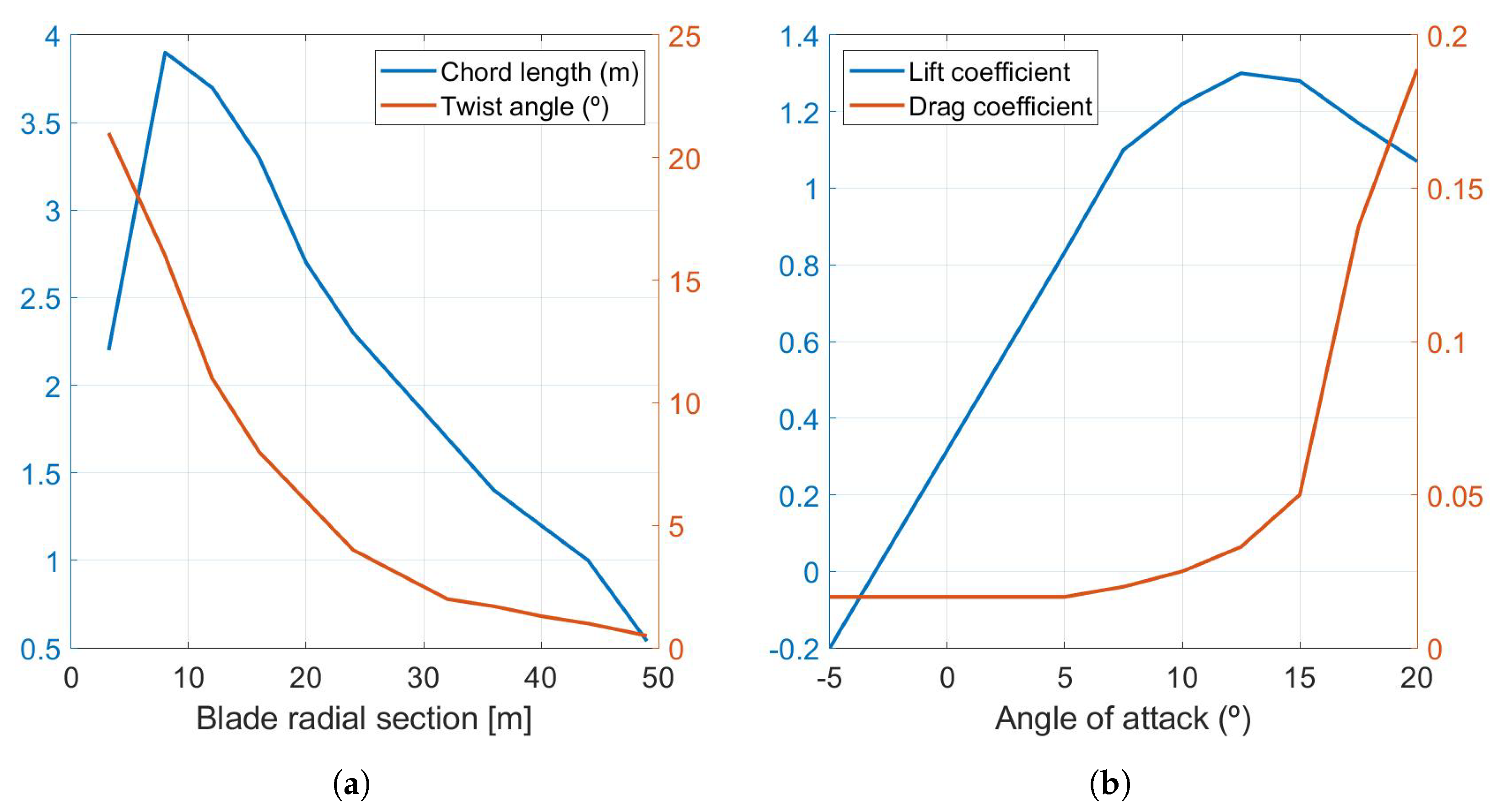
For the ALM implementation, the chord length and twist angle distributions were taken from [31], and are depicted in Figure 3a. The airfoil used was the NACA 63-415 for the entire blade. Lift and drag coefficients were also obtained from [31] and the corresponding lift and drag coefficients are presented in Figure 3b. The used smearing factors, normalized by the rotor diameter, are , , and , in the normal, radial and tangential direction respectively.
The inertia of the drive-train was estimated based on [57] considering the rotor diameter, the material it is made of, and the wind turbine rated power, obtaining a value of kgm. Regarding the torque controller, was estimated from the turbines ten-minutes SCADA data, by computing the mean angular speed and mean electric torque at wind speed bins, considering only the below rated range of wind speed. The obtained value was , which differs 25% from the theoretical value in Equation (11), obtained based on the BEM method. In the simulation, the SCADA-obtained value of was used as we think it was a better representation of the actual operation of the wind turbine based on real operational data.
It should be mentioned that the above numerical setup, including a mesh sensitivity study, has been used by the authors in previous studies, with a particular focus on computing the mean power production of each wind turbine at a below rated wind speed, comparing the results with averages obtained after filtering ten-minutes SCADA data according to the simulated wind speed and wind direction. For further details please see [31,32].
The PI blade-pitch controller implementation requires two parameters to be defined, the natural frequency and damping, and the blade-pitch sensitivity. The natural frequency value used is the same as the one considered in [52], but we chose a lower damping value than what was recommended, aiming for the controller response to be similar to what we observed in the 1 Hz of SCADA data. We chose the values of rad/s and . The blade-pitch sensitivity, , was computed as the difference in aerodynamic power () by considering small variations of the pitch angle () around its optimal value divided by . As suggested in [52], we invoked the frozen-wake assumption in the BEM method, in which the induced wake velocities are held constant while the blade-pitch angle is perturbed. To validate this methodology, we also computed it for the 5 MW reference wind turbine, considering the published data in [52]. It was observed that the pitch sensitivity varied nearly linearly with blade pitch angle, so a linear fit could be computed, where is the blade-pitch angle at which the pitch sensitivity doubled from its value at . Based on SCADA data, the pitch-angle was limited by saturation values of [−2, +90], and its maximum rate of change was set to 8/s.
The following values were obtained: and . Considering these values, the obtained gains are: ; . The gain-correction factor, which multiplies each gain and depends on the blade pitch angle, is computed as:
Finally, the following values were considered for these other controller parameters: , , and .
4. Simulation Cases and Results
In this section we present the results of the simulations, focusing on the dynamic of the variables involved in the power controller. The numerical results were compared to 1 Hz of SCADA data acquired at three specifics periods. These periods were selected to show the operation of the wind turbines under various conditions, above and below rated speed, with and without wake interaction as well as with a de-rate operation. It is worth mentioning though that in this work we are not trying to reproduce the exact events that occurred on those specific dates and that we are taking the SCADA data as a reference to show the operation under real conditions. One of the reasons that makes the comparison difficult is that we only have information about the atmospheric conditions at the location from a single meteorological mast, which has cup anemometers at three different heights (please see Figure 2b). Figure 4 shows the temporal evolution of the meteorological variables measured at the meteorological mast and the wind turbines on the day of the event presented in the Section 4.1.
With the meterological mast information it is possible to estimate the vertical profile of the wind speed and turbulence intensity at a given point in the wind farm, but it is not possible to reproduce the same conditions that actually happened. Present and future work is and will be dedicated to accomplish that by coupling the Caffa3d code with the Weather Research & Forecasting (WRF) model. Another fact is that the data acquired by the meteorological mast of the wind farm is recorded on a ten-minutes basis, which is a far larger temporal scale than the one we are considering in the simulations. This means that changes in the atmospheric conditions that may occur within those ten minutes are not recorded by the anemometers, but those changes will imply the controllers to act accordingly. Nevertheless, even if the comparisons between the simulations and 1 Hz of SCADA data are not precise enough because of the mentioned reasons, it is the author’s opinion that it is better to present them, rather than presenting only the numerical results.
In the second part of this section we present numerical results about active power control at the wind turbine level. To evaluate the effect of wake interaction in the power control, we simulated the operation of the wind turbines under several de-rate signals, comparing two wind directions. Results of the individual and total power production of the wind farm are shown.
4.1. Operation without Wake Interaction at above Rated Wind Speed
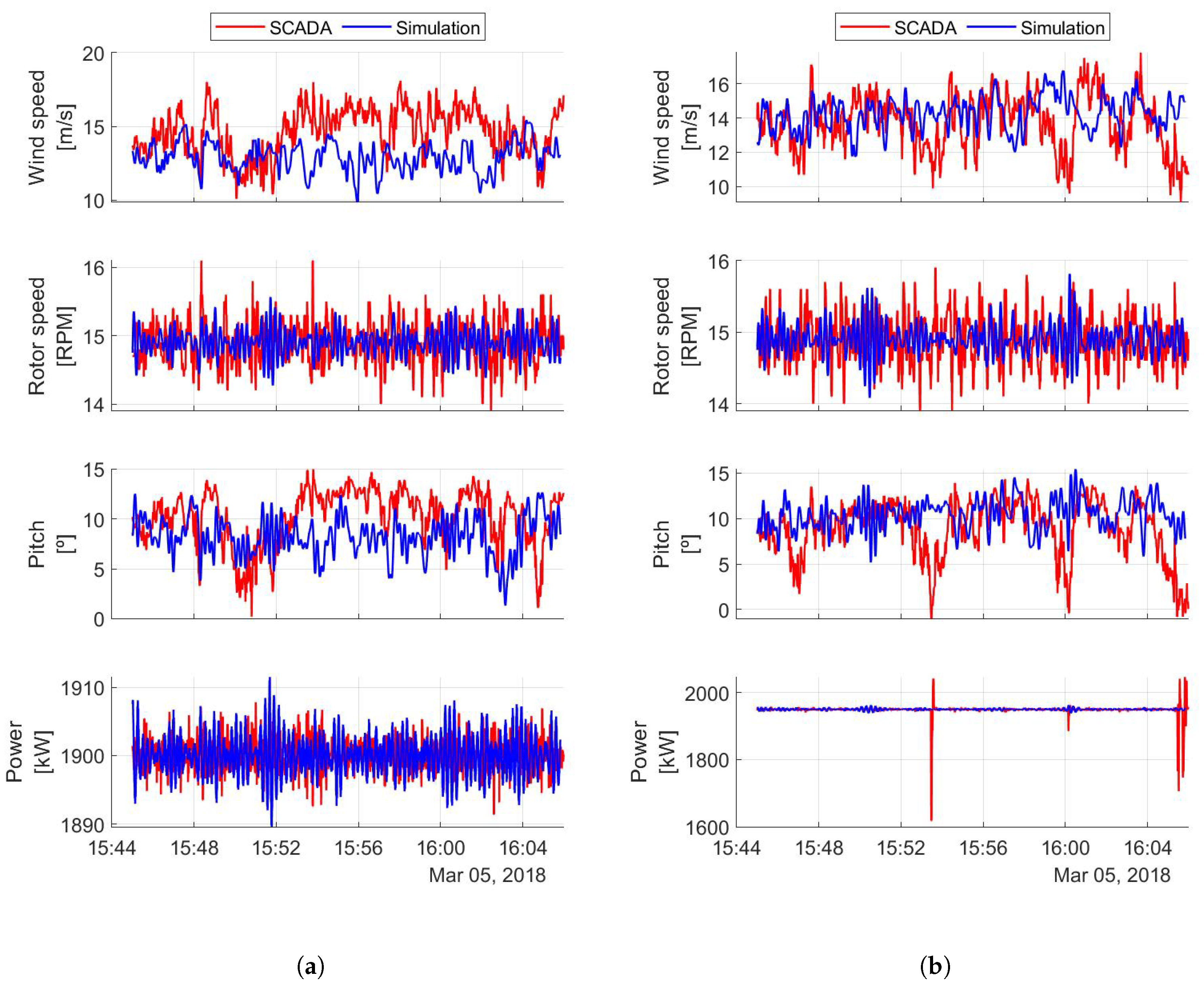
In this section, the wind farm subject to an ABL like inflow condition, from a direction without wake interaction and wind speed above rated is analyzed. Figure 5 depicts the temporal evolution of 1200 s simulation and SCADA data of WT1 and WT2. The SCADA data corresponds to a period starting on the 5 March 2018 at 15.44 h, when the average wind speed at hub height and wind direction were 13 m/s and 264 respectively, according to the meteorological mast measurements (please see Figure 4). The wind direction considered at the simulation was 250, but it is worth noting that in none of these directions (250 and 264) were the wind turbines affected by the wake of another wind turbine. The shown signals are wind speed, rotor angular speed, pitch angle, and electric power. The simulation velocity signal corresponds to the value at the cell located at the inlet of the domain, at hub height and upstream of the corresponding wind turbine position. The SCADA signal is the velocity measured at the wind turbine nacelle.
Looking at the time series, the pitch signals take values above the minimum (−2) during the entire 1200 s period. This shows that the pitch-controller was operating to regulate the angular speed of the rotor, which in turn was fluctuating around its rated value in both the SCADA and simulation signals. As a consequence, the power output of both wind turbines was being controlled around its rated value, as desired. Large peaks were observed in the electric power signal from the SCADA of WT2, both above and below rated speed, which lasted for around 10 s. These peaks may be associated to a sudden change in wind speed, as the pitch angle acted accordingly prior and after the occurrence of these peaks. This in not captured in the simulation, where the wind speed did not change in that way over time. The electric power peaks could also be caused by the operation of electric components (e.g., the inverter or the generator), which we did not consider in our simulation.
Figure 6 shows the histograms of the same signals of Figure 5, for WT1, WT2, and WT3. The vertical dashed lines represent the temporal mean value of each signal. We obtained good agreement between the mean values of the simulation and the SCADA data. For the wind speed and pitch histograms, a somewhat different shape can be observed, being narrower and with a higher peak in the simulation. This can be explained by the fact that, in the simulation, the turbulence intensity was lower than in the real event, 8% and 12% respectively. Nevertheless, the general behavior was well captured, showing the capacity of the numerical framework to model the wind turbine’s operation, including its controller.
4.2. Operation with Wake Interaction at Rated Wind Speed
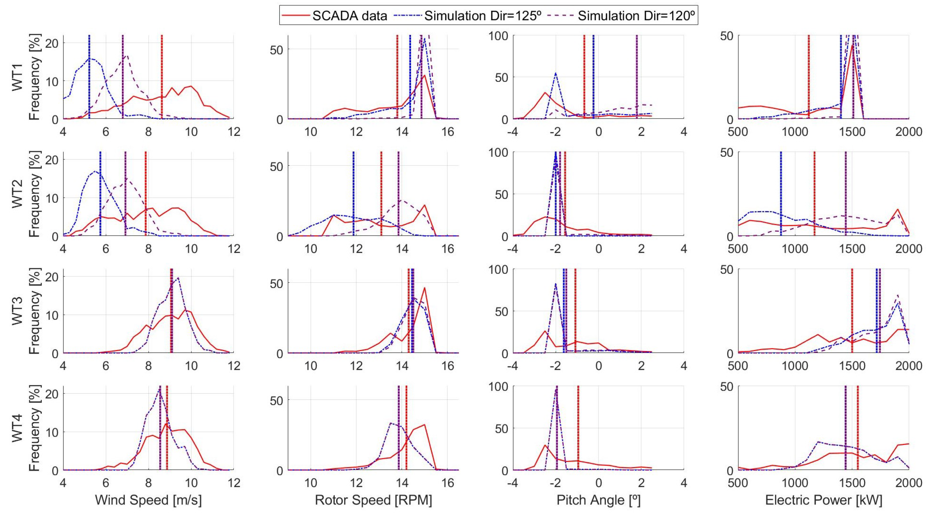
In this section, a second reference case corresponding to the 15 April 2019, between 11.35 and 12.10 h, is considered. During this period the wind direction was between 120 and 125, where WT1 and WT2 were affected by the wake of WT3 (please see Figure 2). This was noticed in the SCADA data of the affected wind turbines by a reduction of their power production and a wind speed deficit at their location. The free wind speed at hub height was between 9 m/s and 10 m/s, being 10 m/s the rated value. Furthermore, during the entire period WT1 was de-rated to 80% of its rated power, that is 1530 kW.
It should be mentioned that, even though in the real event the wind direction was changing, we represented this situation by computing two independent simulations subject to constant wind directions, one at 120 and the other at 125. As pointed out in [58], small changes in wind direction may have large impacts on power production, affecting the wind turbine’s operation. Figure 7 shows the histograms of wind speed, angular speed of the rotor, pitch angle, and electric power of the four wind turbines, comparing 1 Hz of SCADA data and the results of the two simulations. For this case, good agreement between the simulations and SCADA data could be observed for WT3 and WT4, which were the ones that not affected by the wake of other turbines. Furthermore, for that reason, notice that the results of the two simulations were similar for these wind turbines. In both simulations the pitch angle of these wind turbines was frequently in its minimum value, showing that the wind turbines were operating at region 2, trying to optimize their power production. Consistently, the rotational speed of their rotors was below its rated value as well as their power output.
For WT1 and WT2, the results of the simulation with wind direction 120 were quite different to the results of the simulation with wind direction 125. This is expected, since there was a higher wake interaction in these wind turbines for wind direction 125 than for wind direction 120. Due to the wake impingement the wind speed seen by the wind turbines was reduced, WT2 was operating at region 2, keeping its pitch angle at its minimum value and adjusting the generator torque to maximize the power capture looking to operate at an optimal tip speed ratio. The rotational speed of the rotor was below its rated value and its power output was lower than the one of WT3. When looking at WT1, there were some differences in its operation, mainly because WT1 was de-rated. As expected, its pitch angle was a bit larger than the minimum value, while its rotational speed was larger than the one of WT2 and close to rated value, particularly in the simulation with wind direction 120. The wind speed in both simulations was under-estimated with respect to the SCADA data, presenting differences in the mean values of 13% and 37% with 120 and 125 simulations, respectively. Regardless of this, for WT2 the mean values of the SCADA data of electric power, rotor speed, and pitch angle fell between the mean values of the simulations, which shows that on average the operation of this wind turbine was well reproduced.
4.3. Operation with Wake Interaction at Below Rated Wind Speed
The third case also corresponds to the 15 April 2019, between 15.35 and 16.20 hrs. During this period the wind direction was also between 120 and 125, but the free wind speed at hub height was about 7 m/s, which is below rated for all wind turbines. In the same way as presented in Section 4.2, wind direction 125 and wind direction 120 were simulated to consider the effect of the wind direction on the operation of each wind turbine. Figure 8 depicts the histograms of wind speed, rotational speed of the rotor, pitch angle, and electric power of the four wind turbines.
As presented in Section 4.2, the operation of WT3 and WT4 is well captured when looking at their rotor’s angular speed, pitch angle, and power production, as these wind turbines were not affected by the wake of other wind turbines. A main difference with respect to the results presented in Figure 7 is that, as the inflow wind speed was below rated, each wind turbine was operating at region 2 keeping its pitch angle at its minimum. The rotational speeds of the rotor of WT3 and WT4 were quite similar, as these wind turbines were subject to similar inflow conditions without the presence of an upstream wind turbine. When looking further downstream, WT1 and WT2 were operating with a lower angular speed than WT3 and WT4, producing less electric power. Again, WT2 was more affected at a wind direction of 125 than a wind direction of 120, with less rotational speed and power output in the former than in the latter.
4.4. Active Power Control at Wind Turbine Level
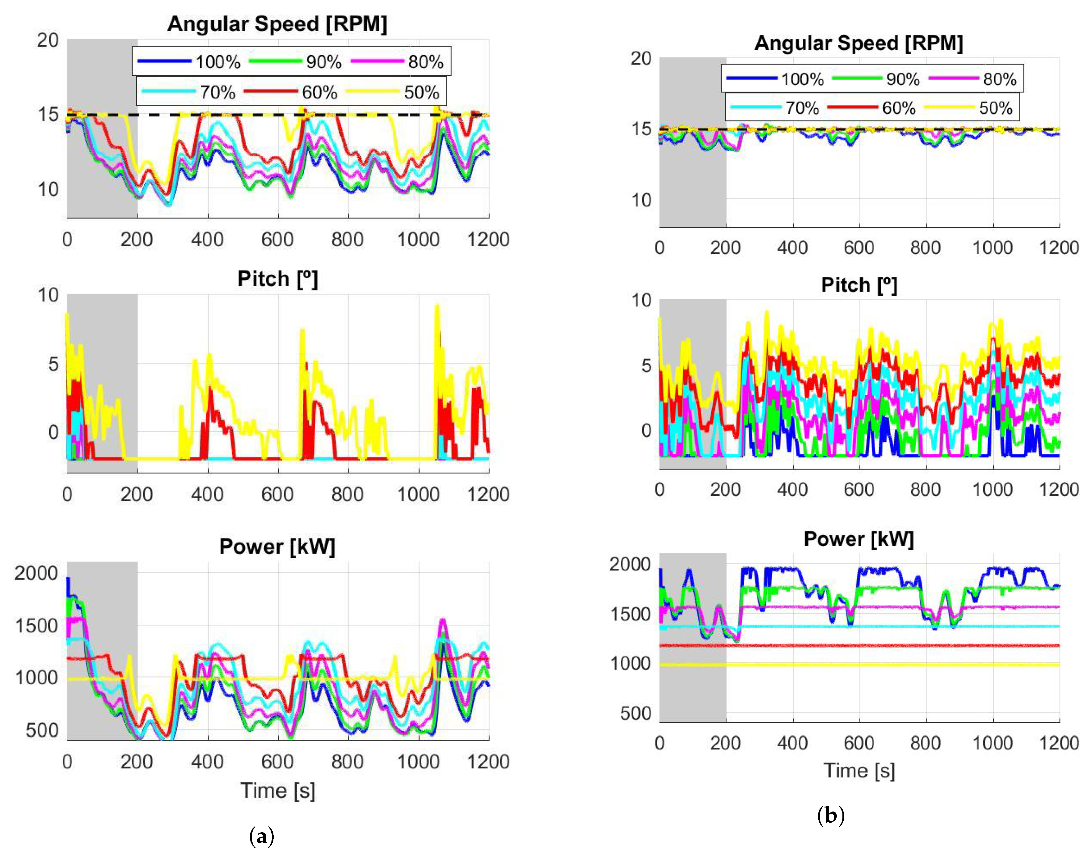
We performed simulations considering several de-rate values for each wind turbine and another wind direction, 147 where WT3 is clearly affected by the wake of WT4 (see Figure 2b). Figure 9a,b show the operation of WT3 and WT4 respectively, at 147, with span-wise averaged velocity of 9 m/s at hub height, considering 6 de-rate commands for both wind turbines: 100%, 90%, 80%, 70%, 60%, and 50%. In the case of WT3 it is clearly noticed that the wind turbine did not reach the required de-rated power, except for some moments when DR = 50% and DR = 60%, when there was enough available power on the wind flow. Furthermore, it can be noticed that the power production of WT3 decreased with higher de-rate values of WT4, as there was less available power due to its wake. The rotor speed was regulated and the pitch angle was kept constant at its minimum value most of the time.
In the case of WT4, the required power was reached in all de-rate levels, although for DR = 100%, 90%, and 80% there were periods where the angular speed did not reach rated value, and thus the generator torque controller operated at region 2, regulating rotor speed to optimize the power extraction from the wind. Again, for lower de-rate commands, higher pitch angles were adopted.
The gray zone at the beginning of the time series represents the first 200 s, and indicates the period affected by transient effects, such as the development of the wakes, due to the sudden inclusion of the wind turbines in the simulations. This can be clearly observed in the angular speed, pitch and power signals of WT3, due to the wake propagation of WT4.
Figure 10 compares results of WT3 operation at 250 and 147 with wind speed at the inlet and hub height of 12 m/s, showing the histograms of rotor speed, pitch angle, and electric power. Two constant de-rate commands were considered: 100% (equivalent to rated power) and 60% . As there was enough wind velocity to reach rated power, for both wind directions, the required levels of electric power could be accomplished, while the rotor speed oscillated around its rated value in both cases. Regarding the pitch angle, higher values were observed at wind direction 250 than at 147 because in the latter case, WT3 was at the wake of WT4 with less available power. Furthermore, higher pitch values were adopted for the 60% de-rate command than for the 100%, for the same wind direction (e.g., 250).
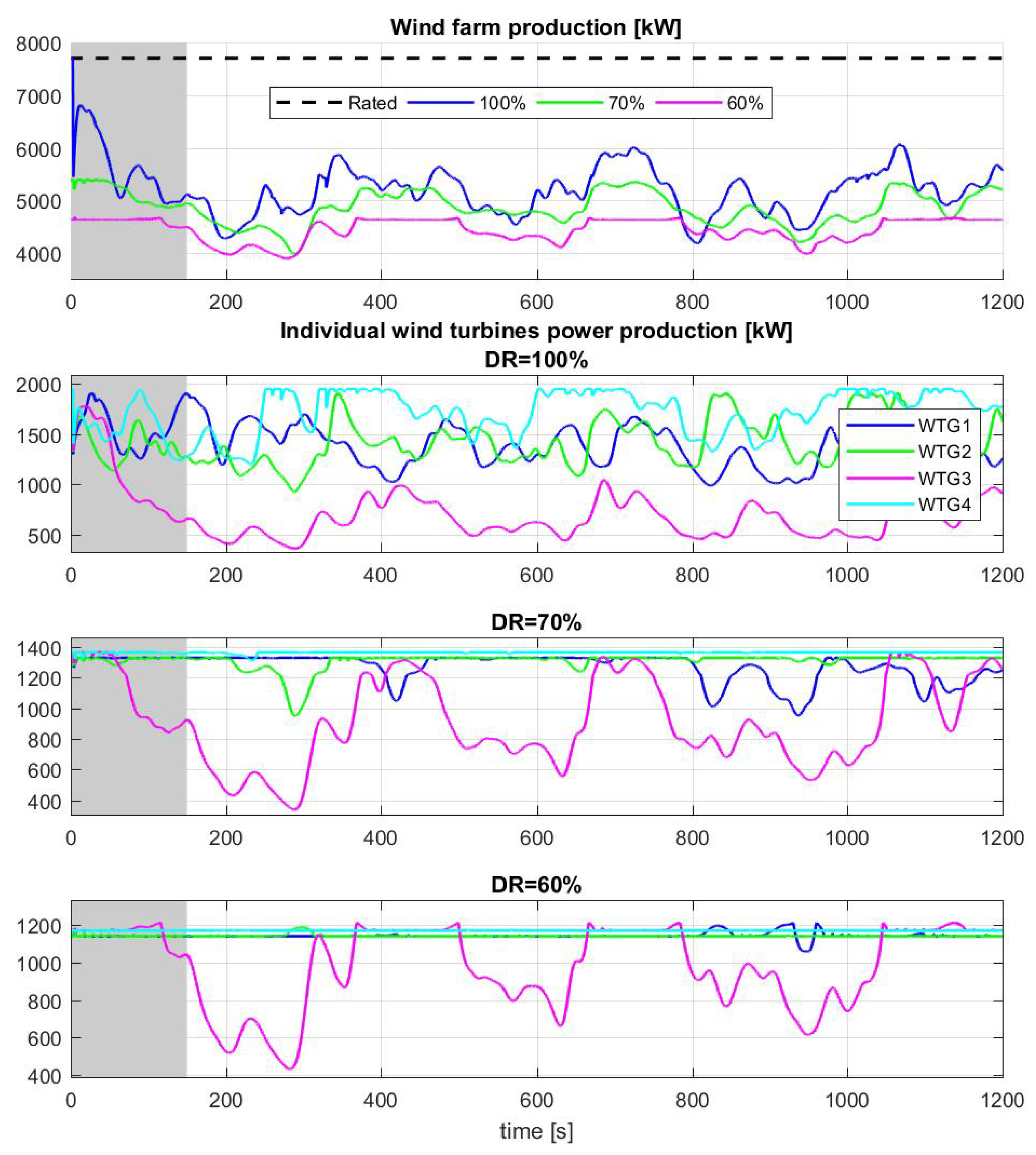
Figure 11 depicts the total wind farm power output, as well from the individual wind turbines, comparing three de-rate levels, for wind direction 147 and wind speed of 9 m/s at hub height at the inlet. The de-rate commands were equally distributed to each wind turbine, regardless of their capacity to reach the desired power output. Only in the case of DR = 50% was the required level reached most of the time. In the other simulations, the power output was not reached mainly because WT3 did not reach its required power as it was strongly affected by WT4 wake. These results show the need to implement a global wind farm controller, with the purpose of assigning de-rate commands based on the available power of each wind turbine, particularly when there are wind turbines operating in the wake of others. Different types of global controllers were studied in [54,55], where they evaluate the effect on the total power output, considering an open-loop or a closed-loop global controller, and it is planned to implement those in Caffa3d.
5. Conclusions and Future Work
A Large Eddy Simulation framework with the Actuator Line Model was used to simulate the operation of a 7.7 MW onshore wind farm. The simulations considered different ABL wind profiles at the inlet, with hub height velocities below and above the rated one, and also considered two different wind directions, one of them with strong interaction between wakes and wind turbines. A closed-loop collective-pitch controller and a torque controller were implemented in the CFD code based on the one presented in [52]. The results of the simulations were compared to high frequency data (1 Hz) from the wind farm SCADA system, obtaining good agreement, both regarding the mean values and the temporal evolution of the signals. The ALM was shown to be capable of simulating with a moderately computational cost, compared with a FRS, the wind flow through wind turbines and wind farms. The ALM proved to be a complementary tool to the models currently applied by the industry, such as the BEM method, as it was envisioned by [7].
The response of the controller subject to different de-rate values, both constant and time-varying, was evaluated. We showed that when there was enough wind power in the flow, the individual wind turbines could follow the required signal, but when it came to the total wind farm power output, it failed to accomplish what was required because of the interaction between wakes and turbines. These results show the necessity of implementing a global controller, which takes into account the available power of each individual wind turbine, which we plan to work on in the near future. In addition to this, work is currently underway to couple the mesoscale model Weather Research and Forecasting (WRF) with the Caffa3d code so as to complement the available microscale measurements, looking to simulate an actual event. A structural model is also planned to be coupled to the LES-ALM approach presented.
Besides, the flow solver, including the wind turbine modules, is being expanded to use GPU computing platforms, as presented in [59], employing a dual CUDA/OpenCL syntax on top of the coarse MPI parallelization. Tests performed have shown speedups of up to 30x with respect to the same simulation executed using CPU platforms.
Author Contributions
Conceptualization, A.G. and M.D.; Data curation, A.G.; Formal analysis, A.G. and M.D.; Methodology, A.G. and M.D.; Validation, A.G.; Writing—original draft, A.G. and M.D.
Funding
This research was funded by the Agencia Nacional de Investigación e Innovación - Fondo Sectorial de Energía (ANII FSE).
Conflicts of Interest
The authors declare no conflict of interest. The funders had no role in the design of the study; in the collection, analyses, or interpretation of data; in the writing of the manuscript, or in the decision to publish the results.
Abbreviations
The following abbreviations are used in this manuscript:
| APC | Active Power Control |
| LES | Large Eddy Simulation |
| ALM | Actuator Line Model |
| BEM | Blade Element Momentum |
| WT | Wind Turbine |
References
- IRENA. Renewable Capacity Statistics 2018; Technical Report; International Renewable Energy Agency: Abu Dhabi, UAE, 2018. [Google Scholar]
- Wind Europe. Wind Energy in Europe in 2018; Technical Report; WindEurope: Brussels, Belgium, 2018. [Google Scholar]
- Ministerio de Energia Industria y Mineria. In Balance Energético Nacional Uruguay—Preliminar; 2018.
- Serrano-González, J.; Lacal-Arántegui, R. Technological evolution of onshore wind turbines—A market-based analysis. Wind Energy 2016, 19, 2171–2187. [Google Scholar] [CrossRef]
- Wiser, R.; Jenni, K.; Seel, J.; Baker, E.; Hand, M.; Lantz, E.; Smith, A. Expert elicitation survey on future wind energy costs. Nat. Energy 2016, 1, 16135. [Google Scholar] [CrossRef]
- Vrana, T.K.; Flynn, D.; Gomez-Lazaro, E.; Kiviluoma, J.; Marcel, D.; Cutululis, N.; Smith, J.C. Wind power within European grid codes: Evolution, status and outlook. Wiley Interdiscip. Rev. Energy Environ. 2018, 7, e285. [Google Scholar] [CrossRef]
- Hansen, M.O.L.; Sørensen, J.N.; Voutsinas, S.; Sørensen, N.; Madsen, H.A. State of the art in wind turbine aerodynamics and aeroelasticity. Prog. Aerosp. Sci. 2006, 42, 285–330. [Google Scholar] [CrossRef]
- Hansen, M.O.; Madsen, H.A. Review paper on wind turbine aerodynamics. J. Fluids Eng. 2011, 133, 114001. [Google Scholar] [CrossRef]
- Sørensen, J.N. Aerodynamic aspects of wind energy conversion. Annu. Rev. Fluid Mech. 2011, 43, 427–448. [Google Scholar] [CrossRef]
- Bai, C.J.; Wang, W.C. Review of computational and experimental approaches to analysis of aerodynamic performance in horizontal-axis wind turbines (HAWTs). Renew. Sustain. Energy Rev. 2016, 63, 506–519. [Google Scholar] [CrossRef]
- Sanderse, B.; Van der Pijl, S.; Koren, B. Review of computational fluid dynamics for wind turbine wake aerodynamics. Wind Energy 2011, 14, 799–819. [Google Scholar] [CrossRef] [Green Version]
- Li, Y.; Castro, A.; Martin, J.; Sinokrot, T.; Prescott, W.; Carrica, P. Coupled computational fluid dynamics/ multibody dynamics method for wind turbine aero-servo-elastic simulation including drivetrain dynamics. Renew. Energy 2017, 101, 1037–1051. [Google Scholar] [CrossRef]
- Sayed, M.; Klein, L.; Lutz, T.; Krämer, E. The impact of the aerodynamic model fidelity on the aeroelastic response of multi-megawatt wind turbine. Renew. Energy 2019, 140, 304–318. [Google Scholar] [CrossRef]
- Bak, C.; Zahle, F.; Bitsche, R.; Kim, T.; Yde, A.; Henriksen, L.C.; Hansen, M.H.; Blasques, J.P.A.A.; Gaunaa, M.; Natarajan, A. The DTU 10-MW reference wind turbine. Danish Wind Power Research 2013 2013. [Google Scholar]
- Jimenez, A.; Crespo, A.; Migoya, E.; García, J. Advances in large-eddy simulation of a wind turbine wake. J. Phys. Conf. Ser. 2007, 75, 012041. [Google Scholar] [CrossRef]
- Wu, Y.T.; Porté-Agel, F. Large-Eddy Simulation of Wind-Turbine Wakes: Evaluation of Turbine Parametrisations. Bound.-Layer Meteorol. 2010, 138, 345–366. [Google Scholar] [CrossRef]
- Sorensen, J.N.; Shen, W.Z. Numerical Modeling of Wind Turbine Wakes. J. Fluids Eng. 2002, 124, 393. [Google Scholar] [CrossRef]
- Shen, W.Z.; Sørensen, J.N.; Zhang, J. Actuator surface model for wind turbine flow computations. In Proceedings of the 2007 European Wind Energy Conference and Exhibition, Milan, Italy, 7–10 May 2007. [Google Scholar]
- Sørensen, J.N.; Mikkelsen, R.F.; Henningson, D.S.; Ivanell, S.; Sarmast, S.; Andersen, S.J. Simulation of wind turbine wakes using the actuator line technique. Philos. Trans. R. Soc. A Math. Phys. Eng. Sci. 2015, 373, 20140071. [Google Scholar] [CrossRef] [PubMed] [Green Version]
- Martínez-Tossas, L.A.; Churchfield, M.J.; Leonardi, S. Large eddy simulations of the flow past wind turbines: Actuator line and disk modeling. Wind Energy 2015, 18, 1047–1060. [Google Scholar] [CrossRef]
- Stevens, R.J.A.M.; Martinez-Tossas, L.A.; Meneveau, C. Comparison of wind farm large eddy simulations using actuator disk and actuator line models with wind tunnel experiments. Renew. Energy 2018, 116, 470–478. [Google Scholar] [CrossRef]
- Yang, X.; Sotiropoulos, F.; Conzemius, R.J.; Wachtler, J.N.; Strong, M.B. Large-eddy simulation of turbulent flow past wind turbines/farms: The Virtual Wind Simulator (VWiS). Wind Energy 2015, 18, 2025–2045. [Google Scholar] [CrossRef]
- Churchfield, M.J.; Lee, S.; Moriarty, P.J.; Martinez, L.A.; Leonardi, S.; Vijayakumar, G.; Brasseur, J.G. A large-eddy simulation of wind-plant aerodynamics. In Proceedings of the 50th AIAA Aerospace Sciences Meeting including the New Horizons Forum and Aerospace Exposition, Nashville, TN, USA, 9–12 January 2012. [Google Scholar]
- Wang, J.; Wang, C.; Campagnolo, F.; Bottasso, C.L. Wake behavior and control: Comparison of LES simulations and wind tunnel measurements. Wind Energy Sci. 2019, 4, 71–88. [Google Scholar] [CrossRef]
- Ciri, U.; Petrolo, G.; Salvetti, M.; Leonardi, S. Large-eddy simulations of two in-line turbines in a wind tunnel with different inflow conditions. Energies 2017, 10, 821. [Google Scholar] [CrossRef]
- Martinez-Tossas, L.A.; Churchfield, M.J.; Yilmaz, A.E.; Sarlak, H.; Johnson, P.L.; Sørensen, J.N.; Meyers, J.; Meneveau, C. Comparison of four large-eddy simulation research codes and effects of model coefficient and inflow turbulence in actuator-line-based wind turbine modeling. J. Renew. Sustain. Energy 2018, 10, 033301. [Google Scholar] [CrossRef] [Green Version]
- Jha, P.K.; Churchfield, M.J.; Moriarty, P.J.; Schmitz, S. Guidelines for volume force distributions within actuator line modeling of wind turbines on large-eddy simulation-type grids. J. Sol. Energy Eng. 2014, 136, 031003. [Google Scholar] [CrossRef]
- Porté-Agel, F.; Wu, Y.T.; Lu, H.; Conzemius, R.J. Large-eddy simulation of atmospheric boundary layer flow through wind turbines and wind farms. J. Wind Eng. Ind. Aerodyn. 2011, 99, 154–168. [Google Scholar] [CrossRef]
- Deskos, G.; Piggott, M.D. Mesh-adaptive simulations of horizontal-axis turbine arrays using the actuator line method. Wind Energy 2018, 21, 1266–1281. [Google Scholar] [CrossRef] [Green Version]
- Draper, M.; Guggeri, A.; Usera, G. Modelling one row of Horns Rev wind farm with the Actuator Line Model with coarse resolution. J. Phys. Conf. Ser. 2016, 753, 82028. [Google Scholar] [CrossRef] [Green Version]
- Guggeri, A.; Draper, M.; Usera, G. Simulation of a 7.7 MW onshore wind farm with the Actuator Line Model. J. Phys. Conf. Ser. 2017, 854, 012018. [Google Scholar] [CrossRef] [Green Version]
- Guggeri, A.; Slamovitz, D.; Draper, M.; Usera, G. A High-Fidelity Numerical Framework For Wind Farm Simulations. In Proceedings of the Tenth International Conference on Computational Fluid Dynamics (ICCFD10), Barcelona, Spain, 9–13 July 2018. [Google Scholar]
- Yang, X.; Pakula, M.; Sotiropoulos, F. Large-eddy simulation of a utility-scale wind farm in complex terrain. Appl. Energy 2018, 229, 767–777. [Google Scholar] [CrossRef]
- Breton, S.; Sumner, J.; Sørensen, J.N.; Hansen, K.S.; Sarmast, S.; Ivanell, S. A survey of modelling methods for high-fidelity wind farm simulations using large eddy simulation. Philos. Trans. A Math. Phys. Eng. Sci. 2017, 375, 20160097. [Google Scholar] [CrossRef] [PubMed] [Green Version]
- Usera, G.; Vernet, A.; Ferré, J.A. A Parallel Block-Structured Finite Volume Method for Flows in Complex Geometry with Sliding Interfaces. Flow Turbul. Combust. 2008, 81, 471. [Google Scholar] [CrossRef]
- Mendina, M.; Draper, M.; Kelm Soares, A.P.; Narancio, G.; Usera, G. A general purpose parallel block structured open source incompressible flow solver. Clust. Comput. 2014, 17, 231–241. [Google Scholar] [CrossRef]
- Ferziger, J.H.; Peric, M. Computational Methods for Fluid Dynamics, 3rd ed.; Springer: Berlin/Heidelberg, Germany, 2002. [Google Scholar]
- Liao, C.C.; Chang, Y.W.; Lin, C.A.; McDonough, J.M. Simulating flows with moving rigid boundary using immersed-boundary method. Comput. Fluids 2010, 39, 152–167. [Google Scholar] [CrossRef]
- Lilek, Ž.; Muzaferija, S.; Perić, M.; Seidl, V. An implicit finite-volume method using nonmatching blocks of structured grid. Numer. Heat Transf. 1997, 32, 385–401. [Google Scholar] [CrossRef]
- Smagorinsky, J. General circulation experiments with the primitive equations: I. The basic experiment. Mon. Weather Rev. 1963, 91, 99–164. [Google Scholar] [CrossRef]
- Mason, P.J.; Thomson, D.J. Stochastic backscatter in large-eddy simulations of boundary layers. J. Fluid Mech. 1992, 242, 51–78. [Google Scholar] [CrossRef]
- Germano, M.; Piomelli, U.; Moin, P.; Cabot, W.H. A dynamic subgrid-scale eddy viscosity model. Phys. Fluids A Fluid Dyn. 1991, 3, 1760–1765. [Google Scholar] [CrossRef]
- Zang, Y.; Street, R.L.; Koseff, J.R. A dynamic mixed subgrid-scale model and its application to turbulent recirculating flows. Phys. Fluids A Fluid Dyn. 1993, 5, 3186–3196. [Google Scholar] [CrossRef]
- Porte-Agel, F.; Meneveau, C.; Parlange, M.B. A scale-dependent dynamic model for large-eddy simulation: application to a neutral atmospheric boundary layer. J. Fluid Mech. 2000, 415, 261–284. [Google Scholar] [CrossRef] [Green Version]
- Draper, M. Simulación del Campo de Vientos y de la Interacción Entre Aerogeneradores. Ph.D. Thesis, Universidad de la República, Montevideo, Uruguay, 2015. [Google Scholar]
- Draper, M.; Usera, G. Evaluation of the Actuator Line Model with coarse resolutions. J. Phys. Conf. Ser. 2015, 625, 12021. [Google Scholar] [CrossRef] [Green Version]
- Draper, M.; Guggeri, A.; Usera, G. Validation of the Actuator Line Model with coarse resolution in atmospheric sheared and turbulent inflow. J. Phys. Conf. Ser. 2016, 753, 82007. [Google Scholar] [CrossRef]
- Draper, M.; Guggeri, A.; Mendina, M.; Usera, G.; Campagnolo, F. A Large Eddy Simulation-Actuator Line Model framework to simulate a scaled wind energy facility and its application. J. Wind Eng. Ind. Aerodyn. 2018, 182, 146–159. [Google Scholar] [CrossRef]
- Draper, M.; Guggeri, A.; Mendina, M.; Usera, G.; Campagnolo, F. A Large Eddy Simulation model for the study of wind turbine interactions and its application. In Proceedings of the Tenth International Conference on Computational Fluid Dynamics (ICCFD10), Barcelona, Spain, 9–13 July 2018. [Google Scholar]
- Guggeri, A.; Draper, M.; Usera, G.; Campagnolo, F. An Actuator Line Model Simulation of two semi-aligned wind turbine models, operating above-rated wind speed. In Proceedings of the Tenth International Conference on Computational Fluid Dynamics (ICCFD10), Barcelona, Spain, 9–13 July 2018. [Google Scholar]
- Mühle, F.; Schottler, J.; Bartl, J.; Futrzynski, R.; Evans, S.; Bernini, L.; Schito, P.; Draper, M.; Guggeri, A.; Kleusberg, E.; et al. Blind test comparison on the wake behind a yawed wind turbine. Wind Energy Sci. 2018, 3, 883–903. [Google Scholar] [CrossRef] [Green Version]
- Jonkman, J.; Butterfield, S.; Musial, W.; Scott, G. Definition of a 5-MW Reference wind Turbine for Offshore System Development; Technical Report; National Renewable Energy Laboratory (NREL): Golden, CO, USA, 2009. [Google Scholar]
- Hansen, M.O. Aerodynamics of Wind Turbines; Earthscan Publications Ltd.: London, UK, 2015. [Google Scholar]
- Fleming, P.; Aho, J.; Gebraad, P.; Pao, L.; Zhang, Y. Computational Fluid Dynamics Simulation Study of Active Power Control in Wind Plants. In Proceedings of the 2016 American Control Conference (ACC), Boston, MA, USA, 6–8 July 2016; pp. 1413–1420. [Google Scholar]
- van Wingerden, J.W.; Pao, L.; Aho, J.; Fleming, P. Active Power Control of Waked Wind Farms. IFAC-PapersOnLine 2017, 50, 4484–4491. [Google Scholar] [CrossRef]
- Guggeri, A.; Draper, M.; Lopez, B.; Usera, G. Actuator Line Model simulations to study active power control at wind turbine level. J. Phys. Conf. Ser. 2019, 1256, 012030. [Google Scholar] [CrossRef]
- González Rodríguez, A.G.; González Rodríguez, A.; Burgos Payán, M. Estimating Wind Turbines Mechanical Constants. RE&PQJ 2007, 1, 9–11. [Google Scholar]
- Porté-Agel, F.; Wu, Y.T.; Chen, C.H. A numerical study of the effects of wind direction on turbine wakes and power losses in a large wind farm. Energies 2013, 6, 5297–5313. [Google Scholar] [CrossRef]
- Igounet, P.; Alfaro, P.; Usera, G.; Ezzatti, P. Towards a finite volume model on a many-core platform. Int. J. High Perform. Syst. Archit. 2012, 4, 78–88. [Google Scholar] [CrossRef]
Figure 1.
Iteration scheme and LES-ALM coupling for one time step (adapted from [36]).
Figure 1.
Iteration scheme and LES-ALM coupling for one time step (adapted from [36]).

Figure 2.
Libertad wind farm location (a) and layout (b). The arrows indicate the simulated wind directions (adapted from [56]).
Figure 2.
Libertad wind farm location (a) and layout (b). The arrows indicate the simulated wind directions (adapted from [56]).

Figure 3.
Actuator Line Model (ALM) chord length and twist angle distribution (a) and aerodynamic coefficients (b).
Figure 3.
Actuator Line Model (ALM) chord length and twist angle distribution (a) and aerodynamic coefficients (b).

Figure 4.
Wind direction (top) and wind velocity (bottom) ten minute averages, acquired by the meteorological mast and the four wind turbines on 5 March, 2018. The grey area indicates the simulated period when the numerical results are compared with 1 Hz of SCADA data (not shown in this figure).
Figure 4.
Wind direction (top) and wind velocity (bottom) ten minute averages, acquired by the meteorological mast and the four wind turbines on 5 March, 2018. The grey area indicates the simulated period when the numerical results are compared with 1 Hz of SCADA data (not shown in this figure).

Figure 5.
(a)

Figure 6.
Histograms of wind speed (m/s), rotor angular speed (RPM), pitch angle (), and electric power (kW) from the SCADA data and simulation of wind turbines WT1, WT2, and WT3. Inflow condition of the simulation: Wind direction 250 (no wake interaction) and wind speed above rated. Vertical dashed lines represent the mean value of each signal.

Figure 7.
Histograms of wind speed (m/s), rotor angular speed (RPM), pitch angle (), and electric power (kW) from the SCADA data and simulation of wind turbines WT1, WT2, WT3, and WT4. Inflow condition of the simulation: Wind direction 120 and 125 (wake interaction) and wind speed close to rated. Vertical dashed lines represent the mean value of each signal.

Figure 8.
Histograms of wind speed (m/s), rotor angular speed (RPM), pitch angle (), and electric power (kW) from the SCADA data and simulation of wind turbines WT1, WT2, WT3, and WT4. Inflow condition of the simulation: Wind direction 120 and 125 (wake interaction) and wind speed below rated. Vertical dashed lines represent the mean value of each signal.

Figure 9.
(a)

Figure 10.
WT3 operation. Inflow condition of the simulations: Wind direction 250 and wind direction 147 (without and with wake interaction respectively) and wind speed above rated. Two constant de-rated signals applied, 100% (top) and 60% (bottom).
Figure 10.
WT3 operation. Inflow condition of the simulations: Wind direction 250 and wind direction 147 (without and with wake interaction respectively) and wind speed above rated. Two constant de-rated signals applied, 100% (top) and 60% (bottom).

Figure 11.
Power production of the wind farm (top) and of each individual wind turbine. Inflow condition of the simulation: Wind direction 147 (wake interaction between wind turbines) and wind speed below rated. Three constant de-rated signals applied on each wind turbine.
Figure 11.
Power production of the wind farm (top) and of each individual wind turbine. Inflow condition of the simulation: Wind direction 147 (wake interaction between wind turbines) and wind speed below rated. Three constant de-rated signals applied on each wind turbine.

© 2019 by the authors. Licensee MDPI, Basel, Switzerland. This article is an open access article distributed under the terms and conditions of the Creative Commons Attribution (CC BY) license (http://creativecommons.org/licenses/by/4.0/).
Share and Cite
MDPI and ACS Style
Guggeri, A.; Draper, M. Large Eddy Simulation of an Onshore Wind Farm with the Actuator Line Model Including Wind Turbine’s Control below and above Rated Wind Speed. Energies 2019, 12, 3508. https://doi.org/10.3390/en12183508
AMA Style
Guggeri A, Draper M. Large Eddy Simulation of an Onshore Wind Farm with the Actuator Line Model Including Wind Turbine’s Control below and above Rated Wind Speed. Energies. 2019; 12(18):3508. https://doi.org/10.3390/en12183508
Chicago/Turabian StyleGuggeri, Andrés, and Martín Draper. 2019. "Large Eddy Simulation of an Onshore Wind Farm with the Actuator Line Model Including Wind Turbine’s Control below and above Rated Wind Speed" Energies 12, no. 18: 3508. https://doi.org/10.3390/en12183508
Note that from the first issue of 2016, this journal uses article numbers instead of page numbers. See further details here.