Acoustic Impedance Inversion Using Gaussian Metropolis–Hastings Sampling with Data Driving

Abstract

The Markov chain Monte Carlo (MCMC) method based on Metropolis–Hastings (MH) sampling is a popular approach in solving seismic acoustic impedance (AI) inversion problem, as it can improve the inversion resolution by statistical prior information. However, the sampling function of the traditional MH sampling is a fixed parameter distribution. The parameter ignores the statistical information of AI that expands sampling range and reduces the inversion efficiency and resolution. To reduce the sampling range and improve the efficiency, we apply the statistical information of AI to the sampling function and build a Gaussian MH sampling with data driving (GMHDD) approach to the sampling function. Moreover, combining GMHDD and MCMC, we propose a novel Bayesian AI inversion method based on GMHDD. Finally, we use the Marmousi2 data and field data to test the proposed method based on GMHDD and other methods based on traditional MH. The results reveal that the proposed method can improve the efficiency and resolution of impedance inversion than other methods.

1. Introduction

Acoustic impedance (AI) is an important rock property that relates closely to lithology and porosity [1,2]. Lithology and porosity can evaluate the volume of oil and gas directly in the reservoir [3,4]. Consequently, obtaining AI from the seismic data is a significant research activity in geophysics. Several methods are applied to invert AI, such as the Band-limited inversion [5], the linear inversion [6,7], and the sparse-spike inversion [8,9,10]. However, these methods employ only the seismic data and ignore the other useful prior information. It leads to the low-resolution inversion results.

Bayesian inference makes use of prior information from the known rock properties. It provides an approach to improve the resolution of the inversion result [11], thus Bayesian inference is widely adopted in seismic inversion such as pro-stack inversion [3,12,13] and pre-stack inversion [14,15,16]. In AI inversion, the Bayesian AI forward model was proposed. This model uses the posterior probability density function (PDF) and the prior PDF to represent the seismic data and the prior knowledge of rock property and combines the posterior and prior PDF and builds a maximum likelihood estimation problem to represent the AI inversion problem. To solve this problem, many methods are proposed, such as the simulated annealing [17,18,19], the genetic algorithm [20,21,22], the ant-colony algorithms [23,24,25], and the particle swarm algorithms [26,27,28]. However, these methods use the data of impedance and ignore the distribution of impedance [29].

The Monte Carlo Markov Chain method (MCMC) based on Metropolis–Hastings sampling (MH) builds a stable Markov Chain to approximate distribution of impedance. It not only uses the data of impedance, but also applies the distribution of impedance, thus the MCMC method based on MH is widely adopted in AI inversion. Godfrey et al. applied the Markov chains in AI inversion and pointed out the Markov chains can fill in a portion of the low-frequency gap that is absent in most algorithms [30]. Mosegaard et al. employed the MCMC method in seismic reflection inversion and obtained new and significant information [31]. Rosec et al. used the MCMC method in deconvolution and got a high-resolution inversion result [32]. Chen adopted the MCMC in pre-stack impedance inversion and obtained a result with more information [33]. However, the sampling function and discriminant function from MH are not unique. Consequently, the study of these two functions can further improve the efficiency and accuracy of inversion.

Several methods are used to change the sampling function and discriminant function of MH, such as delayed rejection adaptive metropolis (DRAM) MCMC [33], Langevin MCMC [34], Hamiltonian Monte Carlo (HMC) [35]. In AI inversion, Hong et al. adopted the genetic algorithm in MH and improved efficiency and accuracy by the scales from the genetic algorithm [36]. Martin et al. implemented the DRAM-MCMC, the Langevin MCMC and the HMC in AI inversion and applied the Stochastic Newton method to MH that improves the inversion efficiency by local gradient and Hessian information [37]. Zhu et al. employed the reversible jump in MH and avoided strong parameterization [38]. Li et al. applied differential evolution to MH and increased the robustness of the inversion result [39]. However, the sampling functions of the aforementioned methods are fixed parameter distributions. This approach ignores the statistical information of AI which can further improve the efficiency and resolution of inversion result.

In this paper, we apply the statistical information of AI to the sampling function through a Gaussian distribution and build a Gaussian MH sampling with data driving (GMHDD). Then, we combine MCMC and GMHDD, and propose an AI inversion method based on GMHDD. Finally, several experiments are carried out on the Marmousi2 model data and field data. The results show the proposed method based on GMHDD outperforms the other methods based on traditional MH in efficiency and accuracy.

2. Methodology

2.1. Forward Model

The Bayesian AI forward model uses the Bayesian theory to establish the relationship between post-stack observed seismic data and AI [11]. The relationship is indicated by a conditional PDF $p(\mathit{l}|\mathit{s})$, where $\mathit{l}\in {ℝ}^n$ is shown as

$$\mathit{l}=\mathit{ln}(\mathit{z}),$$

(1)

where $\mathit{z}\in {ℝ}^n$ is AI, $\mathit{s}$ represents the observed seismic data. However, this conditional PDF cannot be represented by an independent distribution. Consequently, we express this PDF by Bayes rule. It is represented by

$$p(\mathit{l}|\mathit{s})=p(l)p(s|l)/p(s),$$

(2)

where $p(l)$ denotes the probability distribution of $l$, $p(s|l)$ represents the probability distribution of $s$, when $l$ is known. $p(s)$ denotes the probability distribution of $s$, $p(l|s)$ represents the probability distribution of $l$, when $s$ is known. Thus the distribution of $p(\mathit{l}|\mathit{s})$ is related to the distribution of $p(l)p(s|l)$ as shown in Equation (3).

$$p(\mathit{l}|\mathit{s})\propto p(l)p(s|l).$$

(3)

With respect to $p(s|l)$, the relationship between $s$ and $l$ should be supplied. Reflection coefficient provides a bridge to relate these two vectors. Based on the convolution Equation [40], we build the model between post-stack seismic data and reflection coefficient that is shown by

$$\mathit{s}=\mathit{w}\ast \mathit{r}+\mathit{n},$$

(4)

where $s\in {ℝ}^{(m+n-1)\times 1}$ denotes the seismic data, $\omega \in {ℝ}^{m\times 1}$ is the wavelet, $r\in {ℝ}^{(n-1)\times 1}$ represents the reflection coefficient, $n\in {ℝ}^{(m+n-1)\times 1}$ denotes the random noise, and $\ast$ is the convolution operator. When $r$ is no more than 0.3, $r$ can be solved by the impedance [41]. The relationship is obtained from

$$r_i=\frac{1}{2}(l_{\mathit{i}+1}-l_i),$$

(5)

where $r_i$ is the i-th element of $r$, $l_i$ is the i-th element of $l$. Fortunately, the seismic reflection coefficient is about 0.2 [8], thus Equation (5) can be employed in the seismic data. Also, Equation (5) can be rewritten as a matrix

$$r=\frac{1}{2}\times B\times l,$$

(6)

where $B\in {ℝ}^{(n-1)\times n}$ denotes the difference matrix defined by

$$B={\left(\begin{array}{ccccc}-1& 1& 0& \cdots & 0\\ 0& -1& 1& \ddots & ⋮\\ ⋮& \ddots & \ddots & \ddots & 0\\ 0& \cdots & \cdots & -1& 1\end{array}\right)}_{(n-1)\times n}.$$

(7)

Combining Equation (4) with (6), we can obtain the mathematical model between $s$ and $l$ shown by

$$s=\frac{1}{2}(w\ast (B\times l))+n,$$

(8)

Using the matrix operation to replace the convolution operation, Equation (8) can be rewritten as

$$s=\frac{1}{2}(W\times B\times l)+n,$$

(9)

where $W\in {ℝ}^{(m+n-1)\times (n-1)}$ denotes the convolution matrix from $w$ represented by

$$W={\left(\begin{array}{cccc}{w}_1& 0& \cdots & 0\\ ⋮& w_1& \ddots & ⋮\\ w_m& ⋮& \ddots & 0\\ 0& w_m& ⋮& w_1\\ ⋮& \ddots & \ddots & ⋮\\ 0& \cdots & \ddots & w_m\end{array}\right)}_{(m+n-1)\times (n-1)},$$

(10)

where $w_i$ is the i-th element of $w$, $m$ represents the number of $w$. The Gaussian white noise is used to represent $n$ [42], thus the PDF of $n$ is obtained from

$$p(n)=\frac{1}{(\sqrt{2\pi {\delta }_n}{)}^{n+m-1}}\mathit{exp}(-\frac{{\Vert n\Vert }_2^2}{2{\delta }_n^2}),$$

(11)

${\delta }_n{}^2$ indicates the variance expressed as

$${\delta }_n{}^2=({\displaystyle \sum _{i=1}^{n+m-1}{n}_i^2})/(n+m-1).$$

(12)

To proceed further, we interpret $p(s|l)$ as a likelihood function, expressed as Equation (13).

$$p(s|l)=\frac{1}{(\sqrt{2\pi {\delta }_n}{)}^{n+m-1}}\mathit{exp}(-\frac{{\Vert s-\frac{1}{2}WBl\Vert }_2^2}{2{\delta }_n^2}),$$

(13)

Thus, the distribution $s-\frac{1}{2}WBl$ is assumed to be a Gaussian. Then, we have to assign the PDF of $p(l)$. The distribution of $l$ can also be approximated as a Gaussian distribution [27]. Consequently, Gaussian distribution is employed to represent $p(l)$ that is shown by

$$p(l)=\frac{1}{(\sqrt{2\pi {\delta }_l}{)}^n}\mathit{exp}(-\frac{{\Vert l-{\mu }_l\Vert }_2^2}{2{\delta }_l^2}),$$

(14)

where ${\mu }_l, {\delta }_l{}^2$ are the mean and variance of the logarithmic impedance $l$.

$${\mu }_l=({\displaystyle \sum _{i=1}^n{l}_i})/n,$$

(15)

$${\delta }_l^2=({\displaystyle \sum _{i=1}^n{(l_i-{\mu }_l)}^2})/n.$$

(16)

Combining Equation (13) with (14), we obtain an expression for the distribution of impedance when seismic data are known. $p(\mathit{l}|\mathit{s})$ is represented by

$$p(\mathit{l}|\mathit{s})\propto p(l)p(s|l)=\frac{1}{(\sqrt{2\pi {\delta }_l}{)}^n}\mathit{exp}(-\frac{{\Vert l-{\mu }_l\Vert }_2^2}{2{\delta }_l^2})\frac{1}{(\sqrt{2\pi {\delta }_n}{)}^{n+m-1}}\mathit{exp}(-\frac{{\Vert s-\frac{1}{2}WBl\Vert }_2^2}{2{\delta }_n^2}),$$

(17)

We simplify Equation (17) and introduce weighting factors in the forward model, thus the forward model is presented by

$$p(\mathit{l}|\mathit{s})=\mathit{Cexp}(-C_1{\Vert l-{\mu }_l\Vert }_2^2-C_2{\Vert s-\frac{1}{2}WBl\Vert }_2^2),$$

(18)

where $C$ is a constant, $C_1, C_2$ represent the weighting factors.

2.2. Metropolis–Hastings Sampling

The MCMC method based on MH is a popular method to solve the inversion problem. It includes three steps. First, it builds a sampling function to get a new sample. Second, it calculates the likelihood function of the old and new samples by the Bayesian theorem. Third, it introduces a discriminant function by the likelihood function to select the sample and forms a Markov chain which satisfies the steady state. Finally, it calculates the mean of the part of the Markov chain as the inversion result. The iteration process of MH about vector $l$ is proposed in Algorithm 1.

Algorithm 1 The process of Metropolis–Hastings (MH) sampling about vector $l$

Input: initial parameter $l$, length of Markov Chain N, length of part of Markov Chain $\Delta t.$ Output: inversion result $\tilde{l}.$ 1: The initial value $l^1=l;$ 2: Compute $p(\mathit{l}|\mathit{s});$ 3: For t = 1,…..N do 4: Compute the sample $l^{\mathit{new}}$ from the sampling function $q(l^t,l^{\mathit{new}});$ 5: Compute the PDF $p(l^{\mathit{new}}|s);$ 6: Compute discriminant function $a(l^t,l^{\mathit{new}})=\mathit{min}\left\{\frac{p(l^{\mathit{new}}|\mathit{s})q(l^{\mathit{new}},l^t)}{p(l^t|s)q(l^t,l^{\mathit{new}})},1\right\};$ 7: Compute the value $u\propto u(0,1);$ 8: Compute $l^{t+1}=\{\begin{array}{cc}{l}^t& u>a(l^t,l^{\mathit{new}})\\ l^{\mathit{new}}& u\le a(l^t,l^{\mathit{new}})\end{array};$ 9: End for 10: $\tilde{\mathit{l}}={\displaystyle \sum _{i=n-\Delta t+1}^n{l}^i/\Delta t}.$

2.3. Bayesian AI Inversion Based on GMHDD

As indicated from Algorithm 1, the choice of sampling function influences the efficiency and accuracy of the inversion. However, the traditional sampling function ignores the statistical information of the impedance which can improve efficiency and accuracy. Consequently, we need to analyse the statistical information of the impedance including mean and variance. Moreover, we propose a GMHDD approach to the sampling function that is obtained from

$$q(l^t,l^{\mathit{new}})\propto N(0,{\delta }_l),$$

(19)

Thus, the relationship between $l^t$ and $l^{\mathit{new}}$ is indicated by

$$l^{\mathit{new}}=l^t+\Delta l,\Delta l\propto N(0,{\delta }_l).$$

(20)

We employ the novel inversion method based on GMHDD. It is worth noting that the seismic data are two-dimensional but the above method is applied in one-dimension. So we extract the seismic data $S$ by the trace and employ the novel method in seismic data of each trace $\mathit{s}=\mathit{S}(i)$. Based on Equation (20), we renew the impedance $l^{\mathit{new}}$ from $l^t$. To build the discriminant function, we compute the forward model of $l^t$, $l^{\mathit{new}}$.

$$p(l^t|\mathit{s})=\mathit{Cexp}(-C_1{\Vert l-{\mu }_l\Vert }_2^2-C_2{\Vert s-\frac{1}{2}WB{l}^t\Vert }_2^2),$$

(21)

$$p(l^{\mathit{new}}|s)=\mathit{Cexp}(-C_1{\Vert l-{\mu }_l\Vert }_2^2-C_2{\Vert s-\frac{1}{2}WB{l}^{\mathit{new}}\Vert }_2^2).$$

(22)

Combining Equation (21) with Equation (22), we apply the discriminant function that is defined by

$$a(l^t,l^{\mathit{new}})=\min \left\{\frac{p(l^{\mathit{new}}|s)q(l^{\mathit{new}},l^t)}{p(l^t|s)q(l^t,l^{\mathit{new}})},1\right\}.$$

(23)

Opting a random number $u$ by the uniform distribution $u(0,1)$, we update the t+1th logarithmic impedance $l^{t+1}$.

$$l^{t+1}=\{\begin{array}{cc}{l}^t& u>a(l^t,l^{\mathit{new}})\\ l^{\mathit{new}}& u\le a(l^t,l^{\mathit{new}})\end{array}.$$

(24)

Considering a special situation when $q(l^{\mathit{new}},l^t)=q(l^t,l^{\mathit{new}})$, we can obtain $a(l^t,l^{\mathit{new}})=\mathit{min}\left\{\frac{p(l^{\mathit{new}}|s)}{p(l^t|s)},1\right\}$. We can see $l^{t+1}=l^{\mathit{new}}$, if likelihood function $p(l^{\mathit{new}}|s)\ge p(l^t|s)$. It means the method obtains a solution whose likelihood function is maximized. Consequently, this method is a maximum likelihood estimation method in the special situation.

The above steps are repeated to the time $t+\Delta t$, generating the Markov chain $l^1, l^2, \cdots , l^{t+\Delta t}$. Also, we set a parameter $\mathit{tol}$ as the max mean square error between $l^t$ and $l^{t+\Delta t}$ which can ensure the convergence of the inversion result and finish the iteration. If ${\Vert l^{t+\Delta t}-l^t\Vert }_2/{\Vert l^t\Vert }_2\le \mathit{tol}$, $t=t+\Delta t$ and repeated the above steps. If ${\Vert l^{t+\Delta t}-l^t\Vert }_2/{\Vert l^t\Vert }_2>\mathit{tol}$, the result is convergence. We stop the iterations and solve the mean of a portion of Markov chain.

$$\tilde{l}={\displaystyle \sum _{i=t}^{t+\Delta t}{l}^i/\Delta t}.$$

(25)

Finally, repeating the single trace inversion to all traces, we obtained the two-dimensional impedance $Z$.

$$Z(i)=\mathit{exp}(\tilde{l}).$$

(26)

We structure the algorithm framework of the inversion based on GMHDD which is displayed in Algorithm 2.

Algorithm 2 The inversion based on Gaussian MH sampling with data driving (GMHDD)

Input: $C$$,C_1$$,C_2$$,S$$,Z_0$ $\Delta t$$,\mathit{tol}$$,\mathit{trace}.$ Output: Inversion result $Z.$ $\mathrm{Initialize}:t=1,i=1.$ 1: While $i<\mathit{trace}$ 2: Choose the single trace of seismic data $s=S(i)$ and impedance $l^1=\ln (Z_0(i));$ 3: While ${\Vert l^{t+\Delta t}-l^t\Vert }_2/{\Vert l^t\Vert }_2>\mathit{tol}$ 4: Compute likelihood function $p(l^t|s)=\mathit{Cexp}(-C_1{\Vert l^t-{\mu }_l\Vert }_2^2-C_2{\Vert s-\frac{1}{2}WB{l}^t\Vert }_2^2);$ 5: Renew the impedance $l^{\mathit{new}}=l^t+\Delta l,\Delta l\propto n(0,{\delta }_l);$ 6: Compute likelihood function $p(l^{\mathit{new}}|s)=\mathit{Cexp}(-C_1{\Vert l^{\mathit{new}}-{\mu }_l\Vert }_2^2-C_2{\Vert s-\frac{1}{2}WB{l}^{\mathit{new}}\Vert }_2^2);$ 7: Solve the discriminant function $a(l^t,l^{\mathit{new}})=\mathit{min}\left\{\frac{p(l^{\mathit{new}}|s)q(l^{\mathit{new}},l^t)}{p(l^t|s)q(l^t,l^{\mathit{new}})},1\right\};$ 8: Obtain $u\propto U(0,1);$ 9: Get $l^{t+1}=\{\begin{array}{cc}{l}^t& u>a(l^t,l^{\mathit{new}})\\ l^{\mathit{new}}& u\le a(l^t,l^{\mathit{new}})\end{array};$ 10: $t=t+1;$ 11: End 12: Compute the inversion result $\tilde{l}={\displaystyle \sum _{i=t}^{t+\Delta t}{l}^i/\Delta t};$ 13: Compute $Z(i)=\mathit{exp}(\tilde{l});$ 14: End

3. Experiments

In this section, we apply the Marmousi2 model and field data to test the proposed method. We compare the proposed method based on GMHDD with two other methods based on traditional MH intuitively where the sampling functions of traditional MH are Uniform distributions of fixed parameters $U(-1,1)$ named UMH and Gaussian distributions of fixed parameters $N(0,1)$ named GMH. Moreover, we analyse the inversion results objectively through the root mean square error (RMSE) and signal noise ratio (SNR).

3.1. Marmousi2 Model

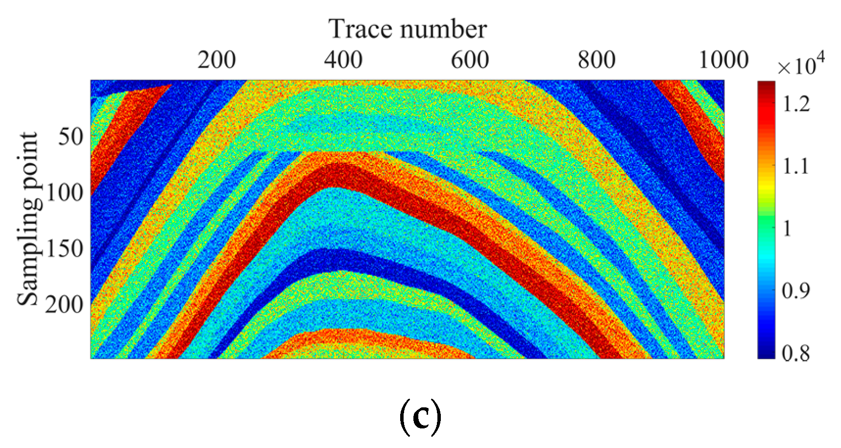
The Marmousi2 model is the most published theoretical model that is used by many researchers in the geophysics [43]. We chose a portion of the Marmousi2 model to compare the proposed method based on GMHDD and other methods based on GMH [44] and UMH [45]. The model includes 1001 traces and each trace has 249 sampling points (depicted in Figure 1a). Based on Equation (5), we obtained the reflection coefficient of the Marmousi2 model (see Figure 1b). Then, we built a 30 Hz main frequency Ricker wavelet and computed the synthetic seismic data of the Marmousi2 model. We add 20% Gaussian white noise in the seismic data to obtain the noisy seismic data. The noisy seismic data are represented in Figure 1c. To improve the efficiency of the inversion, we built an initial model by filtering the true impedance with a Gaussian filter whose size and standard deviation are 51 × 51 and 1 × 10³. The initial model is shown in Figure 1d.

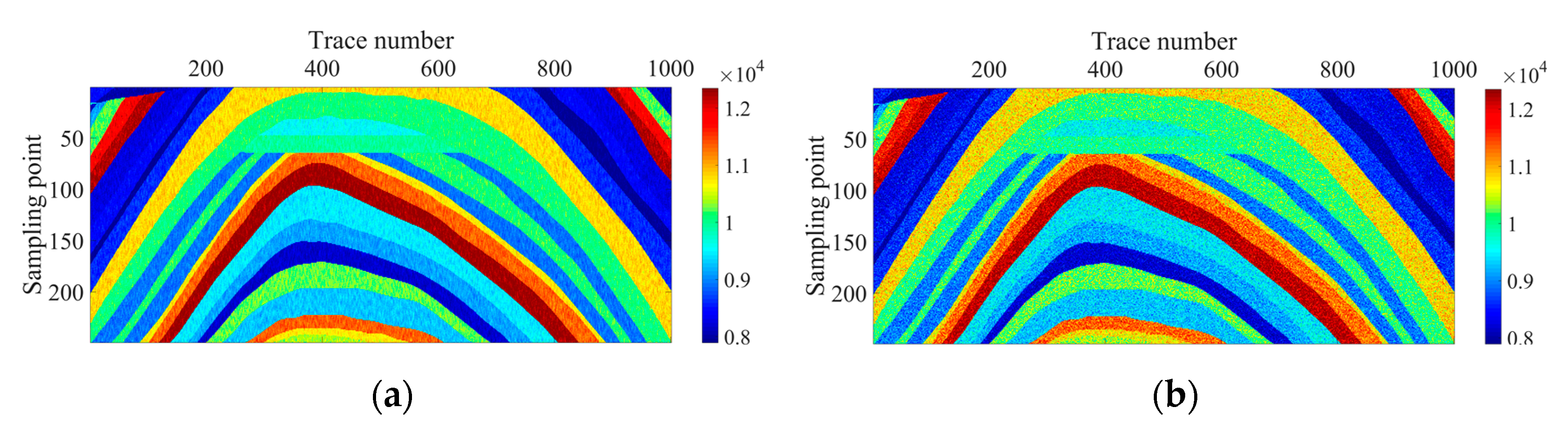
The three methods are used to invert AI of the Marmousi2 model. The inversion result is displayed in Figure 2, where Figure 2a is the inversion result based on GMHDD, Figure 2b is the inversion result based on UMH, Figure 2c is the inversion result based on GMH. It is concluded qualitatively from Figure 2 that the method based on GMH can obtain more robustness result than the method based on UMH, thus the Gaussian distribution is more suitable for AI inversion than the Uniform distribution. Furthermore, the inversion result based on GMHDD is more robustness than that based on GMH.

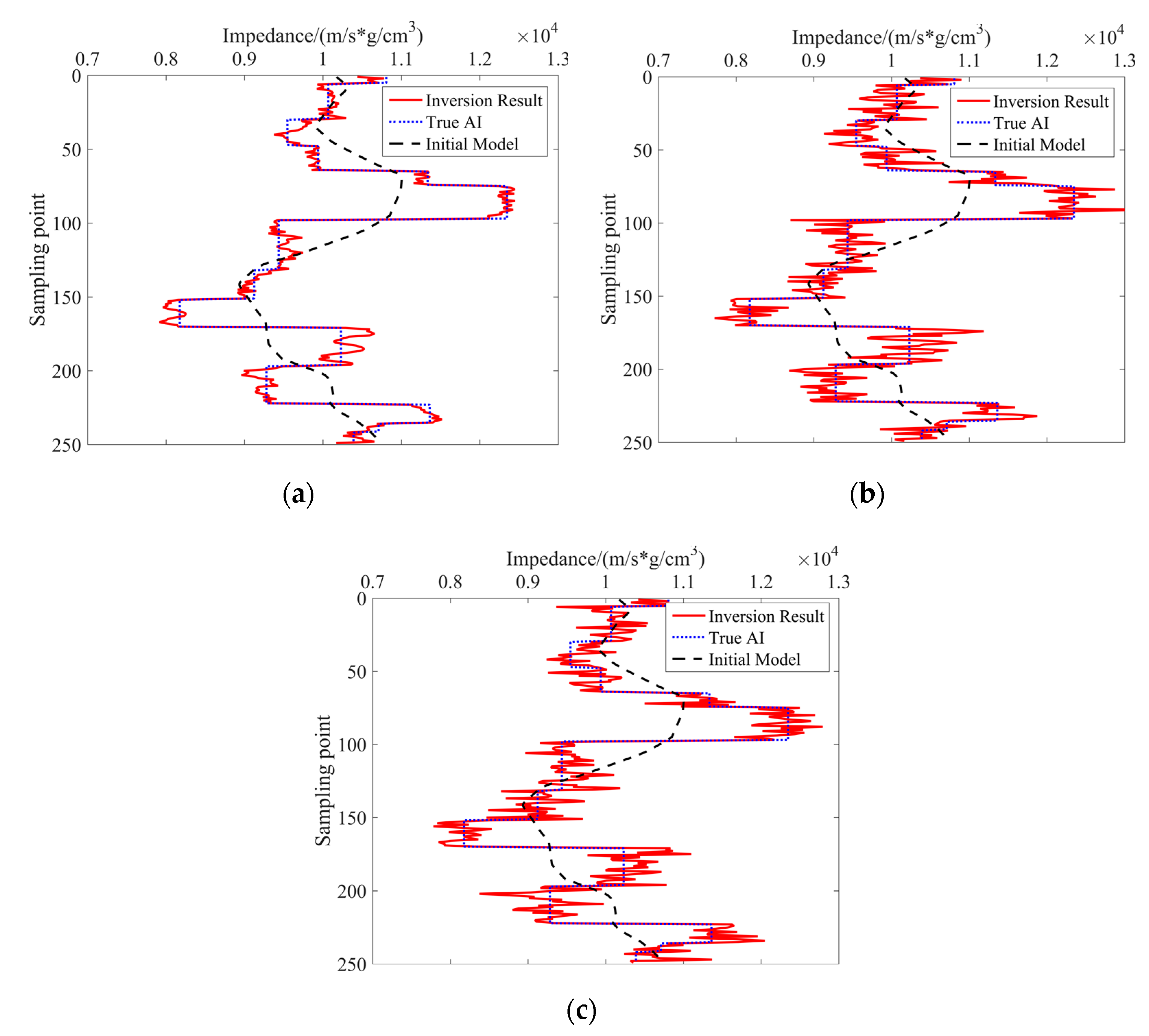
Figure 3 displays single trace inversion results based on three methods, where the red line represents the inversion result, the blue dotted line expresses the initial model, the black dashed line indicates the impedance of the Marmousi2 model. We find in general that the inversion result based on GMHDD is qualitatively more similar to the impedance model than the two other methods. However, the results fluctuate about the true model in Figure 3.

In Figure 4, we present the relationship between the mean square error and the iteration number, where the red line is the relationship based on GMHDD, the green dashed line is the relationship based on GMH, the blue dotted line is the relationship based on UMH. When the iteration number is the same, the mean square error based on GMHDD is lower than the two other methods. This result demonstrates that the proposed method can improve the accuracy of the inversion result. Simultaneously, the iteration number of the proposed method is the lowest in the same mean square error that indicates the proposed method can increase the efficiency of the inversion.

Figure 5 contains the synthetic seismic data of the result based on GMHDD and Marmousi2 model, the noisy synthetic seismic data of the MAarmousi2 model. As shown in Figure 5, the result based on GMHDD is similar to Marmousi2 model. The result means the proposed method performs well in conditions of low SNR of the seismic data.

Table 1. The RMSE, signal noise ratio (SNR) of three methods.

Methods	RMSE (m/s*g/cm3)	SNR (dB)
Initial Model	782.27	6.97
UMH	314.78	15.66
GMH	314.27	15.69
GMHDD	130.26	16.29

shows the RMSE and SNR of each method, where the greatest performances are indicated in bold. It can be illustrated in Table 1 that the proposed method has the lowest RMSE and highest SNR among three methods. These results show the proposed method can improve the accuracy and get an inversion result with less noise.

In general, introducing the statistical information of AI in the sampling function can improve the efficiency and accuracy of the inversion result in the Marmousi2 model. Also, the proposed method based on GMHDD have a good anti-noise ability. However, these results fluctuate about the true model.

3.2. Field Data

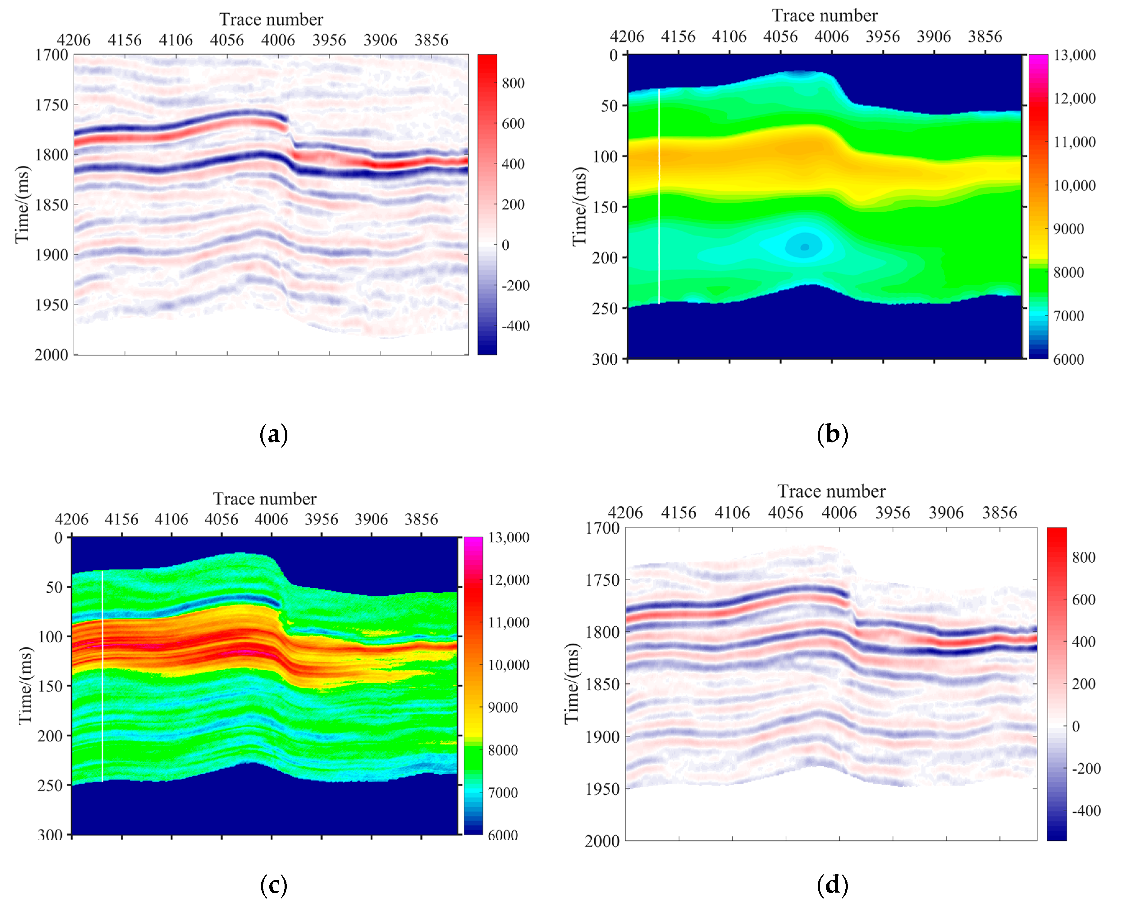
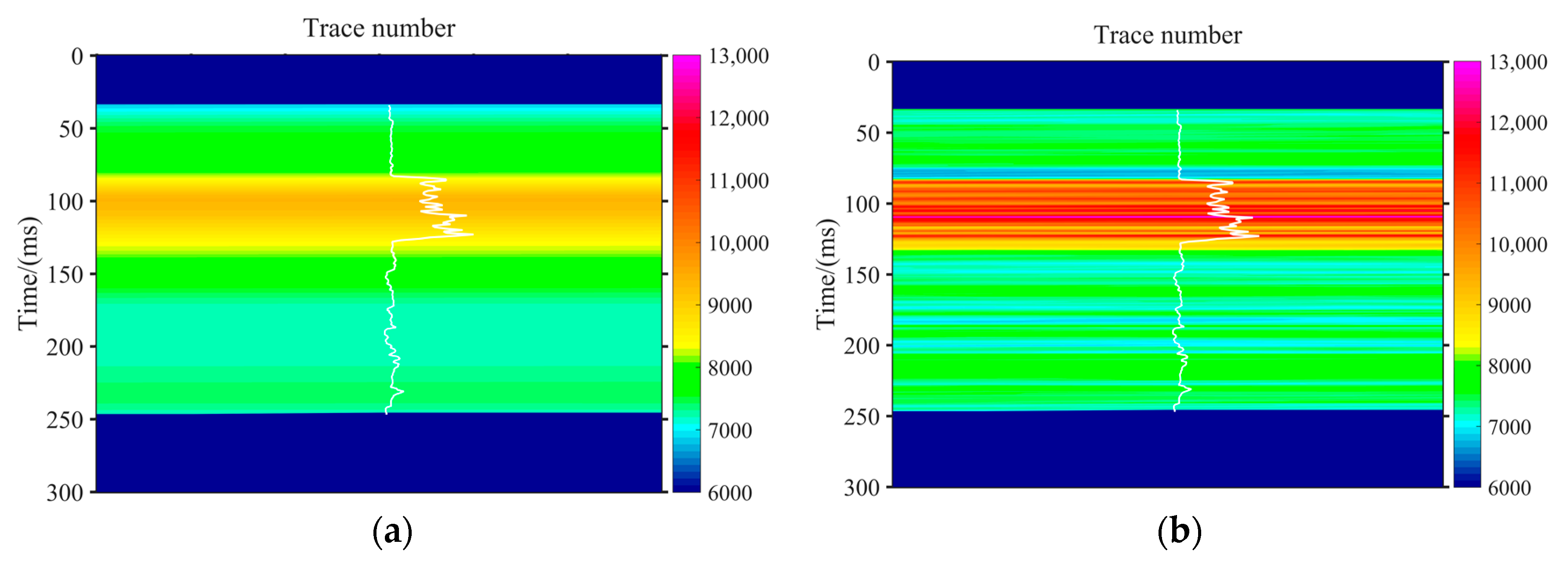
Field data comes from a seismic survey from Africa and is displayed in Figure 6a. It includes 512 traces with 1 ms sampling interval. To get the initial model, we extrapolated the well log by the horizons and filtered the result by the Gaussian filter. The initial model is shown in Figure 6b. We employ the proposed method to invert the field data. The inversion result is represented in Figure 6c, where the white line is a well log. In addition, we synthesize the seismic data by the inversion result of the proposed method. The synthetic seismic data are displayed in Figure 6d. We compared Figure 6b with Figure 6c and found the inversion result of the proposed method includes more information than the initial impedance. This result shows qualitatively that the proposed method can improve the resolution of the impedance. Also, we compared Figure 6a with Figure 6d and found the synthetic seismic data of the inversion result is similar to the seismic record. It expresses the inversion result obeys the field geological law.

In Figure 7, we chose three traces near the well log to analyse the degree of matching between the inversion result and well log. It is concluded from the comparison between Figure 7a with Figure 7b that the layer information of the inversion result near the well log can match well with the peaks and troughs of the well log, where the unit of colors is m/s*g/cm³. It means the inversion results obey the structure of this field data.

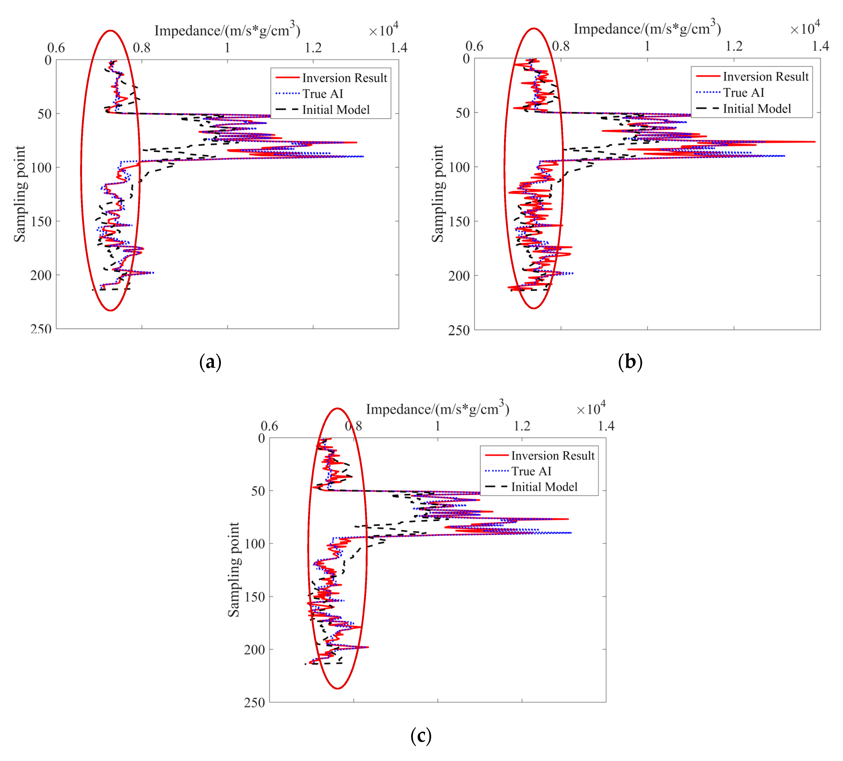
Figure 8 contains a single trace data near the well log based on three methods, where the red line represents the inversion result, the blue dotted line expresses the initial model, the green dashed line indicates the impedance of the well log. As indicated from Figure 8a the inversion result of the proposed method is similar to the impedance near the well log. Also, comparing with the initial model, the resolution of the inversion result is higher. It means the proposed method can get an inversion result with high accuracy and resolution. In addition, comparing Figure 8a with the two other subgraphs, the inversion result of the proposed method appears qualitatively closer to the impedance of the well log than two other methods in the red circle.

We computed the mean square error between the well log and inversion result near the well log and displayed the relationship between the mean square error and the iteration number in Figure 9, where the red line is the relationship based on GMHDD, the green dashed line is the relationship based on GMH, the blue dotted line is the relationship based on UMH. If the mean square error is the same, the iteration number of the proposed method is lowest. It confirms the proposed method can increase the efficiency of the inversion. If the iteration number is the same, the mean square error based on the proposed method is lower than the two other methods. It demonstrated the proposed method can improve the accuracy of the inversion result.

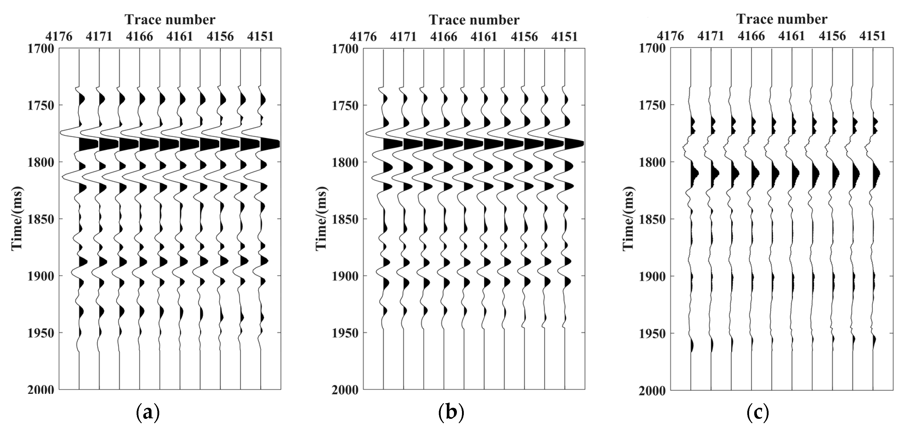
In Figure 10, We synthesized the seismic data by the inversion result of GMHDD and chose 10 traces to compare with the seismic record of the field data. Also, we compute the error between the seismic record of the field data with the synthesize seismic data of the proposed method. We can see from Figure 10 that the error between the seismic record of the field data and the synthesize seismic data of the inversion result is small. It suggests the synthesize seismic data by the proposed method can match the seismic record well and the inversion results obey the law of the observed field data.

Table 2. The RMSE of three methods based on field data.

Methods	Initial Model	UMH	GMH	GMHDD
RMSE (m/s*g/cm3)	819.95	199.16	277.36	158.52

shows the RMSE of three methods based on field data, where the best performances are indicated in bold. Comparing the three methods, the RMSE of the proposed method is lowest among three methods. It indicates the proposed method can improve the accuracy of the inversion results than other traditional methods.

In general, the proposed method based on GMHDD can obtain an inversion result with high accuracy and high resolution in the field data trials. Moreover, the proposed method based on GMHDD improves efficiency and accuracy than two other methods based on traditional MH.

4. Conclusions and Discussion

In this article, we applied statistical information of AI to the sampling function of MH and built a novel GMHDD approach to the sampling function. Moreover, we combine MCMC with GMHDD and proposed a novel Bayesian AI inversion method based on GMHDD. Moreover, we used the Marmousi2 model and field data to test the proposed method based on GMHDD. The results reveal the inversion based on GMHDD has a strong de-noising ability and can improve the efficiency and accuracy of inversion result. We compared the proposed method with two methods based on traditional MH. The results show the inversion based on GMHDD has the highest efficiency and accuracy among the three methods.

In fact, we did not consider the biasedness of the prior distribution in this paper. The bias of the prior has a significantly negative effect on the posterior, thus the biasedness of the prior distribution will be used in our future work [46]. Moreover, we only used the GMHDD in the post-stack seismic data whose incident and reflection are vertical in this paper. However, there are many Bayesian forward models of pre-stack seismic data where the reflection coefficient represents reflections from a stack of layers, such as AVO forward model [14], AVA forward model [47]. Consequently, we will use GMHDD in pre-stack seismic data in future work. Also, we used the Gaussian distribution to build the distribution of impedance. However, there are many methods that use the non-Gaussian distribution to build the distribution of impedance, such as $\alpha$-stable distribution [48], Cauchy distribution [49], and uniform distribution [50]. We will study and apply the non-Gaussian distribution to build the distribution of impedance in future work.

References

- Russell, B.H. Introduction to Seismic Inversion Methods; Society of Exploration Geophysicists: Tulsa, OK, USA, 1988; pp. 34–86. [Google Scholar]
- Li, S.; He, Y.; Chen, Y.; Liu, W.; Yang, X.; Peng, Z. Fast multi-trace impedance inversion using anisotropic total p-variation regularization in the frequency domain. J. Geophys. Eng. 2018, 15, 2171–2182. [Google Scholar] [CrossRef] [Green Version]
- Yue, B.; Peng, Z. Acoustic impedance inversion with covariation approach. J. Inverse Ill-Posed Probl. 2014, 22, 609–623. [Google Scholar] [CrossRef]
- Li, S.; Chen, Y.; Wu, H.; Peng, Z.; Wu, R. Seismic acoustic impedance inversion using total variation with overlapping group sparsity. In Proceedings of the SEG Technical Program Expanded Abstracts 2018, Anaheim, CA, USA, 25–28 September 2018; pp. 411–415. [Google Scholar]
- Bickel, S.H.; Martinez, D.R. Resolution performance of Wiener filters. Geophysics 1983, 48, 887–899. [Google Scholar] [CrossRef]
- Berkhout, A.J. Least-squares inverse filtering and wavelet deconvolution. Geophysics 1977, 42, 1369–1383. [Google Scholar] [CrossRef]
- Li, S.; Peng, Z.; Wu, H. Prestack multi-gather simultaneous inversion of elastic parameters using multiple regularization constraints. J. Earth Sci. 2018, 29, 1359–1371. [Google Scholar] [CrossRef]
- Li, S.; Peng, Z. Seismic acoustic impedance inversion with multi-parameter regularization. J. Geophys. Eng. 2017, 14, 520–532. [Google Scholar] [CrossRef]
- Barrodale, I.; Chapman, N.; Zala, C. Estimation of bubble pulse wavelets for deconvolution of marine seismograms. Geophys. J. Int. 1984, 77, 331–341. [Google Scholar] [CrossRef] [Green Version]
- Barrodale, I.; Zala, C.; Chapman, N. Comparison of the ℓ1 and ℓ2 norms applied to one-at-a-time spike extraction from seismic traces. Geophysics 1984, 49, 2048–2052. [Google Scholar] [CrossRef]
- Box, G.E.; Tiao, G.C. Bayesian Inference in Statistical Analysis; Wiley-Interscience Publication: New York, NY, USA, 1992; pp. 26–61. [Google Scholar]
- Yuan, S.; Wang, S. Spectral sparse Bayesian learning reflectivity inversion. Geophys. Prospect. 2013, 61, 735–746. [Google Scholar] [CrossRef]
- Kormylo, J.J.; Mendel, J.M. Maximum-Likelihood Seismic Deconvolution. IEEE Trans. Geosci. Remote Sens. 2007, 21, 72–82. [Google Scholar] [CrossRef]
- Buland, A.; Omre, H. Bayesian linearized AVO inversion. Geophysics 2003, 68, 185–198. [Google Scholar] [CrossRef] [Green Version]
- Bosch, M.; Mukerji, T.; Gonzalez, E.F. Seismic inversion for reservoir properties combining statistical rock physics and geostatistics: A review. Geophysics 2010, 75, 165–176. [Google Scholar] [CrossRef]
- Peng, Z.; Li, D.; Wu, S.; He, Z.; Zhou, Y. Discriminating gas and water using multi-angle extended elastic impedance inversion in carbonate reservoirs. Chin. J. Geophys. Chin. Ed. 2008, 51, 639–644. [Google Scholar] [CrossRef]
- Ma, X. Simultaneous inversion of prestack seismic data for rock properties using simulated annealing. Geophysics 2002, 67, 1877–1885. [Google Scholar] [CrossRef]
- Srivastava, R.P.; Sen, M.K. Stochastic inversion of prestack seismic data using fractal-based initial models. Geophysics 2010, 75, R47–R59. [Google Scholar] [CrossRef]
- Lindsay, C.E.; Chapman, N.R. Matched field inversion for geoacoustic model parameters using adaptive simulated annealing. IEEE J. Ocean. Eng. 1993, 18, 224–231. [Google Scholar] [CrossRef]
- Gerstoft, P. Inversion of seismoacoustic data using genetic algorithms and a posteriori probability distributions. J. Acoust. Soc. Am. 1994, 95, 770–782. [Google Scholar] [CrossRef]
- Wu, Q.; Wang, L.; Zhu, Z. Research of pre-stack AVO elastic parameter inversion problem based on hybrid genetic algorithm. Clust. Comput. 2017, 20, 3173–3183. [Google Scholar] [CrossRef]
- Padhi, A.; Mallick, S. Accurate estimation of density from the inversion of multicomponent prestack seismic waveform data using a nondominated sorting genetic algorithm. Lead. Edge 2013, 32, 94–98. [Google Scholar] [CrossRef]
- Yuan, S.; Tian, N.; Chen, Y.; Liu, H.; Liu, Z. Nonlinear geophysical inversion based on ACO with hybrid techniques. In Proceedings of the 2008 Fourth International Conference on Natural Computation, Jinan, China, 18–20 October 2008; pp. 530–534. [Google Scholar]
- Conti, C.R.; Roisenberg, M.; Neto, G.S.; Porsani, M.J. Fast seismic inversion methods using ant colony optimization algorithm. IEEE Geosci. Remote Sens. Lett. 2013, 10, 1119–1123. [Google Scholar] [CrossRef]
- Chen, S.; Wang, S.; Zhang, Y. Ant colony optimization for the seismic nonlinear inversion. In SEG Technical Program Expanded Abstracts; Society of Exploration Geophysicists: Tulsa, OK, USA, 2005; Volume 24, p. 2668. [Google Scholar]
- Saraswat, P.; Sen, M.K. Simultaneous stochastic inversion of prestack seismic data using hybrid evolutionary algorithm. In SEG Technical Program Expanded Abstracts; Society of Exploration Geophysicists: Tulsa, OK, USA, 2010; Volume 29, pp. 2850–2854. [Google Scholar]
- Figueiredo, L.P.D.; Grana, D.; Santos, M.; Figueiredo, W.; Roisenberg, M.; Neto, G.S. Bayesian seismic inversion based on rock-physics prior modeling for the joint estimation of acoustic impedance, porosity and lithofacies. J. Comput. Phys. 2017, 336, 128–142. [Google Scholar] [CrossRef]
- Yue, B.; Peng, Z.; Hong, Y.; Zou, W. Wavelet inversion of pre-stack seismic angle-gather based on particle swarm optimization algorithm. Chin. J. Geophys.-Chin. Ed. 2009, 52, 3116–3123. [Google Scholar]
- Peng, Z.; Li, Y.; Wei, W.; He, Z.; Li, D. Nonlinear AVO inversion using particle filter. Chin. J. Geophys.-Chin. Ed. 2008, 51, 862–871. [Google Scholar] [CrossRef]
- Godfrey, R.; Muir, F.; Rocca, F. Modeling seismic impedance with Markov chains. Geophysics 1980, 45, 1351–1372. [Google Scholar] [CrossRef]
- Mosegaard, K.; Singh, S.; Snyder, D.; Wagner, H. Monte Carlo analysis of seismic reflections from Moho and the W reflector. J. Geophys. Res.-Solid Earth 1997, 102, 2969–2981. [Google Scholar] [CrossRef]
- Rosec, O.; Boucher, J.M.; Nsiri, B.; Chonavel, T. Blind marine seismic deconvolution using statistical MCMC methods. IEEE J. Ocean. Eng. 2003, 28, 502–512. [Google Scholar] [CrossRef]
- Haario, H.; Laine, M.; Mira, A.; Saksman, E. DRAM: Efficient adaptive MCMC. Stat. Comput. 2006, 16, 339–354. [Google Scholar] [CrossRef]
- Marshall, T.; Roberts, G. An adaptive approach to Langevin MCMC. Stat. Comput. 2012, 22, 1041–1057. [Google Scholar] [CrossRef]
- Girolami, M.; Calderhead, B. Riemann manifold langevin and hamiltonian monte carlo methods. J. R. Stat. Soc. Ser. B-Stat. Methodol. 2011, 73, 123–214. [Google Scholar] [CrossRef]
- Hong, T.; Sen, M.K. A new MCMC algorithm for seismic waveform inversion and corresponding uncertainty analysis. Geophys. J. Int. 2009, 177, 14–32. [Google Scholar] [CrossRef] [Green Version]
- Martin, J.; Wilcox, L.C.; Burstedde, C.; Ghattas, O. A stochastic Newton MCMC method for large-scale statistical inverse problems with application to seismic inversion. SIAM J. Sci. Comput. 2012, 34, A1460–A1487. [Google Scholar] [CrossRef]
- Zhu, D.; Gibson, R. Seismic inversion and uncertainty quantification using transdimensional Markov chain Monte Carlo method. Geophysics 2018, 83, R321–R334. [Google Scholar] [CrossRef]
- Li, K.; Yin, X.; Liu, J.; Zong, Z. An improved stochastic inversion for joint estimation of seismic impedance and lithofacies. J. Geophys. Eng. 2019, 16, 62–76. [Google Scholar] [CrossRef]
- Russell, B.; Hampson, D. Comparison of poststack seismic inversion methods. In SEG Technical Program Expanded Abstracts; Society of Exploration Geophysicists: Tulsa, OK, USA, 1991; Volume 10, pp. 876–878. [Google Scholar]
- Walker, C.; Ulrych, T.J. Autoregressive recovery of the acoustic impedance. Geophysics 1983, 48, 1338–1350. [Google Scholar] [CrossRef]
- Grana, D.; Fjeldstad, T.; Omre, H. Bayesian Gaussian mixture linear inversion for geophysical inverse problems. Math. Geosci. 2017, 49, 493–515. [Google Scholar] [CrossRef]
- Martin, G.S.; Wiley, R.; Marfurt, K.J. Marmousi2: An elastic upgrade for Marmousi. Lead. Edge 2006, 25, 156–166. [Google Scholar] [CrossRef]
- Gelman, A.; Roberts, G.O.; Gilks, W.R. Efficient Metropolis jumping rules. Bayesian Stat. 1996, 5, 599–608. [Google Scholar]
- Wang, D.; Zhang, G. AVO simultaneous inversion using Markov chain Monte Carlo. In Proceedings of the SEG Technical Program Expanded Abstracts, Denver, CO, USA, 17–22 October 2010; pp. 444–448. [Google Scholar]
- Li, T.; Corchado, J.M.; Bajo, J.; Sun, S.; De Paz, J.F. Effectiveness of Bayesian filters: An information fusion perspective. Inf. Sci. 2016, 329, 670–689. [Google Scholar] [CrossRef]
- Chen, J.; Hoversten, G.M.; Vasco, D.; Rubin, Y.; Hou, Z. A Bayesian model for gas saturation estimation using marine seismic AVA and CSEM data. Geophysics 2007, 72, WA85–WA95. [Google Scholar] [CrossRef]
- Yue, B.; Peng, Z. A validation study of α-stable distribution characteristic for seismic data. Signal Process. 2015, 106, 1–9. [Google Scholar] [CrossRef]
- Yuan, S.Y.; Wang, S.X.; Luo, C.M.; Wang, T.Y. Inversion-Based 3-D Seismic Denoising for Exploring Spatial Edges and Spatio-Temporal Signal Redundancy. IEEE Geosci. Remote Sens. Lett. 2018, 15, 1682–1686. [Google Scholar] [CrossRef]
- Cary, P.W.; Chapman, C.H. Automatic 1-D waveform inversion of marine seismic refraction data. Geophys. J. Int. 2010, 93, 527–546. [Google Scholar] [CrossRef]
Figure 1.
The part of the Marmousi2 model. (a) True acoustic impedance (AI) model; (b) Reflection coefficient; (c) Noisy synthetic seismic and (d) Initial AI model.
Figure 2.
The inversion results. (a) GMHDD; (b) GMH and (c) UMH.
Figure 3.
The inversion results of trace 301. (a) GMHDD; (b) Gaussian distributions of fixed parameters (GMH) and (c) Uniform distributions of fixed parameters (UMH).
Figure 4.
The relationship between the mean square error and iteration number from the three methods.
Figure 5.
The synthetic seismic data. (a) The Marmousi2 model; (b) Noisy data; and, (c) GMHDD.
Figure 6.
Field data. (a) Seismic record; (b) Initial impedance; (c) Inversion result of GMHDD and (d) Synthetic seismic data of GMHDD.
Figure 7.
The impedance near the well log. (a) Initial model and (b) GMHDD.
Figure 8.
The inversion results near the well log. (a) GMHDD; (b) GMH; (c) UMH.
Figure 9.
Figure 10.
Part of seismic data. (a) Field data; (b) GMHDD; (c) Error between field data with GMHDD.