Assessment of Primary Energy Conversion of a Closed-Circuit OWC Wave Energy Converter

Abstract

Tupperwave is a wave energy device based on the Oscillating-Water-Column (OWC) concept. Unlike a conventional OWC, which creates a bidirectional air flow across the self-rectifying turbine, the Tupperwave device uses rectifying valves to create a smooth unidirectional air flow, which is harnessed by a unidirectional turbine. This paper deals with the development and validation of time-domain numerical models from wave to pneumatic power for the Tupperwave device and the conventional OWC device using the same floating spar buoy structure. The numerical models are built using coupled hydrodynamic and thermodynamic equations. The isentropic assumption is used to describe the thermodynamic processes. A tank testing campaign of the two devices at 1/24th scale is described, and the results are used to validate the numerical models. The capacity of the innovative Tupperwave OWC concept to convert wave energy into useful pneumatic energy to the turbine is assessed and compared to the corresponding conventional OWC.

1. Introduction

Waves are an ocean energy resource, which has the potential to contribute in the offshore renewable energy mix. A multitude of different devices have been invented to convert the wave power into electrical power, but the challenges involved in the development of an economically-sustainable solution are huge. No device for large-scale energy production from the waves has yet reached the stage of commercialisation. The barriers include high maintenance costs and survivability in extreme sea states amongst others. Oscillating-Water-Columns (OWCs) are among the most promising wave energy devices because of their relative simplicity. The only moving part being the turbine connected in direct drive to the generator, low levels of maintenance are expected. Moreover, the air contained in the OWC chamber flows across the turbine at high speed, transforming the slow motion and high forces from the waves into a fast rotational speed and low torque at the turbine. This primary conversion of the wave power into pneumatic power acts as a non-mechanical gear-box and constitutes a huge advantage in terms of maintenance and survivability. This feature is not exclusive to OWC device and is found in other wave energy converters that use air as a conversion fluid and flexible membranes such as the sea clam [1] and the Bombora device [2], amongst others. OWC devices are among the most studied type of wave energy technologies, and their principle is used in various forms.

For the most common form of OWC devices, the air flow across the turbine is bidirectional, and the turbine is self-rectifying. Such a turbine can harness both flow directions, but is not as efficient as a unidirectional turbine. State-of-the-art self-rectifying air turbines reach a maximum efficiency in the order of 70–75% in constant flow conditions during scaled tests [3]. In real-sea conditions, the air flow across the turbine is highly fluctuating since it stops and changes direction every 3–5 s. In such conditions, the average efficiency of self-rectifying turbines is 5–10% lower than their maximum efficiency [3]. Other forms of OWCs use non-return valves to rectify the flow in a single direction across a unidirectional turbine. Single-stage unidirectional turbines reach 85–90% efficiency in constant flow conditions [4,5]. The use of rectifying valves was successful for Masuda’s commercial navigation buoy (1965) powered by wave energy [6], but the experience of the Kaimei device [7] in 1986 revealed that there were challenges associated with the use of valves in larger scale devices for power production where air flow rates are in the order of $100{\mathrm{m}}^3·{\mathrm{s}}^{-1}$. Such flow rates necessitate large valve dimensions, which are unsuited for the fast opening and closing response time required for the valves. The moderate success of the Kaimei was also due to the limited theoretical knowledge of wave energy absorption available at the time [8].

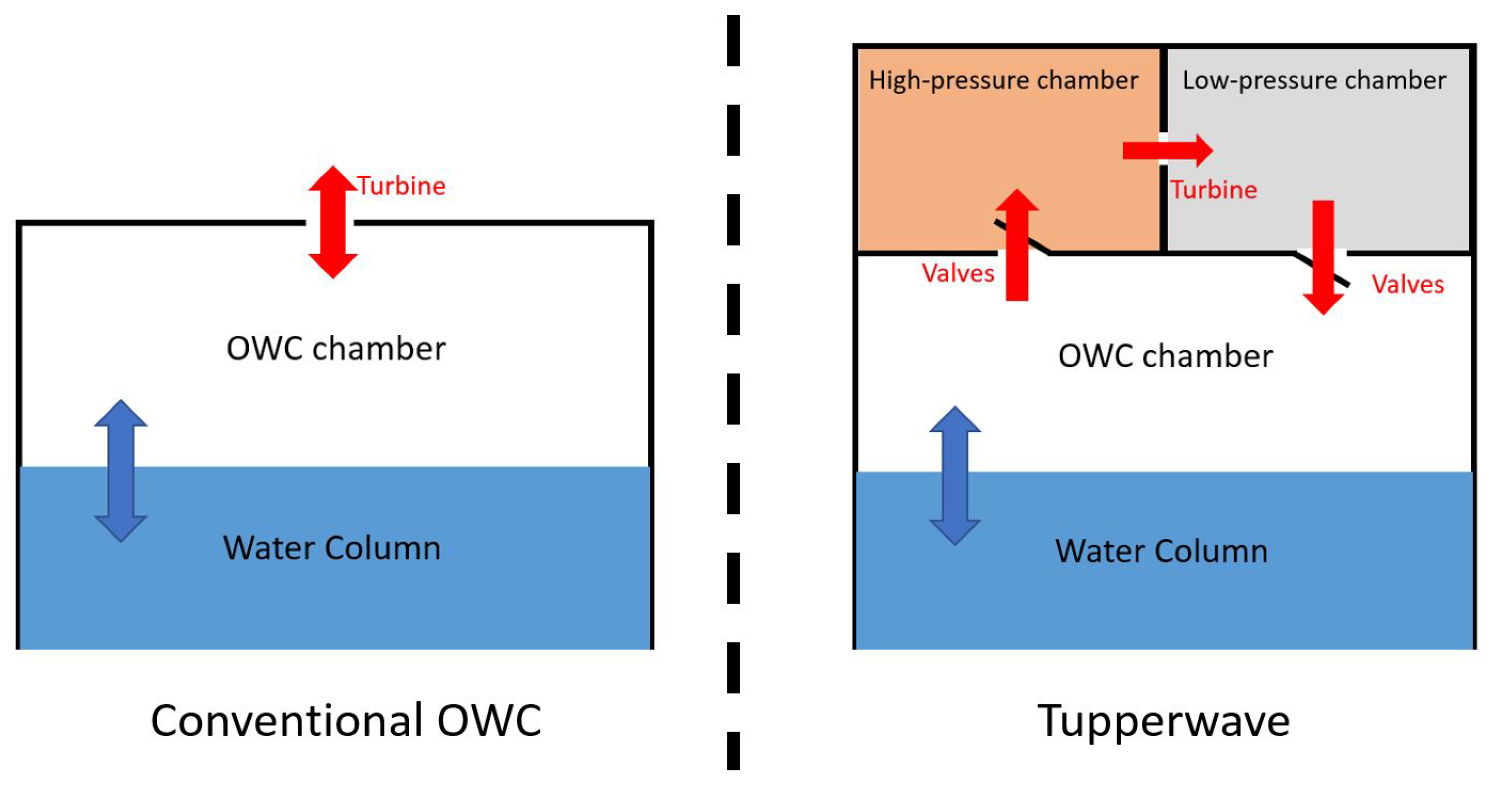
The idea of using a high-efficiency unidirectional turbine in an OWC device is however still appealing since it could potentially increase the device efficiency. The Tupperwave principle suggests another approach on the use of non-return valves for the generation of a closed-circuit air flow. The Tupperwave concept for OWCs consists of self-rectifying valves, two large air chambers that act as accumulators, and a unidirectional turbine. The Tupperwave principle is described in Figure 1 and can be applied to fixed or floating devices.

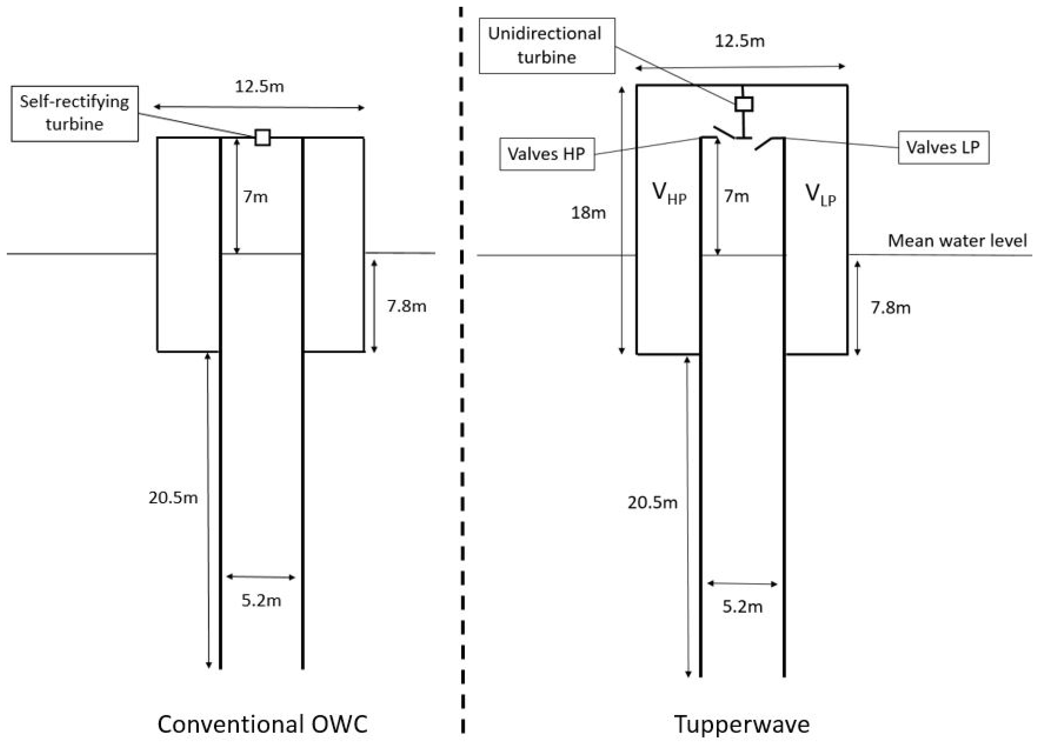
Floating devices are however more suitable because of the available buoyancy volume, which can be divided in two parts and used as the High-Pressure (HP) chamber and Low-Pressure (LP) chambers. In this article, the Tupperwave principle is applied to a floating axisymmetric structure in the form of a spar buoy. In addition to a potential yield increase due to the high efficiency of the unidirectional turbine, this principle also aims at smoothing the flow across the turbine and hence maximising its efficiency and the power quality delivered by the device. An optimization study showed that the volume of these chambers should be maximized [9]. Thus, the whole buoyancy volume of the chosen spar buoy was used, and each chamber was $950{\mathrm{m}}^3$. Figure 2 displays the schematic for the Tupperwave device at full scale, as well as the corresponding conventional OWC using the same spar buoy geometry.

The power conversion chain of wave energy converters is achieved in various stages. In the case of OWC devices, the incoming wave power reaching the device is partly absorbed by the device. This absorbed power is then converted into useful pneumatic power available across the turbine. Finally, the power available to the turbine is converted into electrical power by the turbine and generator system. The development and validation of a model encompassing all power conversion stages is challenging due to complex interdependent physical phenomena happening at each stage and the cost of building a physical model with all the components [10]. Therefore, developers usually decide to study parts of the power conversion chain separately, as in [11,12,13].

In this paper, the first two conversion stages are considered: the Tupperwave device and the corresponding conventional OWC (Figure 2) are numerically modelled from wave to pneumatic power, and the results are validated against tank testing experiments. The objective is to assess, numerically and physically, the capacity of the Tupperwave device to convert wave power into smooth pneumatic power available to the turbine and compare it to the performance of the conventional OWC.

The hydrodynamic and thermodynamic equations forming the devices’ numerical models from wave to pneumatic power are presented in Section 2. Section 3 describes the tank testing experiments carried out. Section 4 compares the physical model performances and the numerical and experimental results of both devices for the validation of the numerical models. Finally, the conclusions of the work are given in Section 5.

2. Numerical Models From Wave to Pneumatic Power

The time-domain numerical models from wave to pneumatic power for the two devices studied in this research consist of a number of coupled differential equations obtained via hydrodynamic and thermodynamic considerations.

2.1. Hydrodynamics

Both the Tupperwave device and the conventional OWC use the same spar buoy geometry. The hydrodynamic model is therefore the same for the two devices. The model is based on linear wave theory, using the assumptions that wave steepness and bodies motions are sufficiently small. To solve the linear hydrodynamic problems in the OWC device, several approaches have been developed. The two most popular approaches are the uniform surface pressure model [14] and the rigid piston model [15]. The former approach is exact because it makes no assumption on the generally warped Internal Water Surface (IWS) and assumes spatially-uniform pressure on the IWS. The latter approach approximates the IWS to be a thin rigid piston moving along the column of the device. This approximation is reasonable when the radius of the IWS is small compared to the wavelength. With this approach, the problem becomes a two-rigid-body problem (device floating structure-rigid piston) that can be solved using the Boundary Element Method (BEM) developed in the 1970s for the study of interaction between waves and floating bodies (ships) [16]. This approach is used in this research.

Spar buoys move essentially in heave due to the relatively large length of the submerged tail tube, and the heave motion is the main contribution for the power conversion of the axisymmetric device. Hence, to simplify the problem, only the heave motions of the two bodies are considered. This assumption is reasonable and commonly adopted in the literature [17,18,19]. The vertical displacement of the device structure and rigid piston are respectively denoted as $(x_1,x_2)$, and the vertical axis is upward. The constant horizontal section of the IWS is denoted as $S_2$. The volume of the OWC chamber, denoted as V, varies with the relative vertical displacement of the bodies. A dot over a variable indicates the variable’s derivative taken with respect to time. When the device is floating at rest on calm water ($x_1=x_2=0$), the OWC chamber has a volume of $V_0$. We therefore have:

$$\left\{\begin{array}{c}V=V_0+S_2(x_1-x_2)\hfill \\ \dot{V}=S_2({\dot{x}}_1-{\dot{x}}_2)\hfill \end{array}\right.$$

(1)

In order to establish a time-domain model of the system’s dynamic response, the hybrid frequency-time domain method described in [20] is used. Each body is subjected to the Cummins equation [21]. The reciprocating pressure force $f_p$ due to the pressure building in the OWC chamber is added, along with the viscous drag force $f_d$. The coupled heave motions of the two-bodies can be written in time-domain as [17]:

$$\left\{\begin{array}{c}[m_1+A_{11}(\infty )]{\ddot{x}}_1\left(t\right)+{\int }_0^t{K}_{11}(t-\tau ){\dot{x}}_1\left(t\right)d\tau +A_{12}(\infty ){\ddot{x}}_2\left(t\right)\hfill \\ +{\int }_0^t{K}_{12}(t-\tau ){\dot{x}}_2\left(t\right)d\tau +c_1{x}_1\left(t\right)=f_1\left(t\right)+f_p\left(t\right)+f_{d1}\left(t\right)+f_{m1}\left(t\right)\left(a\right)\hfill \\ A_{21}(\infty ){\ddot{x}}_1\left(t\right)+{\int }_0^t{K}_{21}(t-\tau ){\dot{x}}_1\left(t\right)d\tau +[m_2+A_{22}(\infty )]{\ddot{x}}_2\left(t\right)\hfill \\ +{\int }_0^t{K}_{22}(t-\tau ){\dot{x}}_2\left(t\right)d\tau +c_2{x}_2\left(t\right)=f_2\left(t\right)-f_p\left(t\right)+f_{d2}\left(t\right)\left(b\right)\hfill \end{array}\right.$$

(2)

where $m_i$ are the bodies masses; $A_{ij}(\infty )$ are the bodies heaving added masses at infinite frequency (including the proper and crossed modes); $c_i$ are the hydrostatic stiffness terms and are calculated as $c_1={\rho }_{w}g{S}_1$ and $c_2={\rho }_{w}g{S}_2$, where ${\rho }_w$ is the water density, g is the acceleration of gravity, $S_1$ is the constant horizontal cross-sectional area of the device structure at the undisturbed sea surface; $K_{ij}$ are the impulse response functions for heave motions; $f_i$ are the wave excitation forces; $f_{m1}$ is the force applied by the mooring system on the device structure.

The impulse response functions can be obtained by the following formula:

$$K_{ij}\left(t\right)={\displaystyle \frac{2}{\pi }}{\int }_0^{\infty }{B}_{ij}\left(\omega \right)cos\left(\omega t\right)d\omega$$

(3)

where $B_{ij}$ is the radiation damping coefficient in the frequency domain.

The excitation forces are calculated as:

$$f_i\left(t\right)={\int }_0^t{K}_{ex,i}(t-\tau )\eta \left(t\right)dt$$

(4)

where $\eta$ is the external wave elevation and $K_{ex,i}$ is the excitation force impulse response function calculated as:

$$K_{ex,i}\left(t\right)=\frac{1}{\pi }{\int }_0^{\infty }Re\left\{{\tilde{F}}_{ex,i}\left(\omega \right)e^{-i\omega t}\right\}d\omega$$

(5)

where ${\tilde{F}}_{ex,i}\left(\omega \right)$ is the excitation force coefficient from the waves on body i. The frequency domain coefficients $A_{ij}(\infty )$, $B_{ij}\left(\omega \right)$, $c_i$, and ${\tilde{F}}_{ex,i}\left(\omega \right)$ are calculated using the commercial BEM solver WAMIT [22].

The reciprocating pressure force is calculated as $f_p=S_2{p}_{owc}\left(t\right)$, and $p_{owc}$ is the excess pressure relative to atmospheric pressure built in the OWC chamber. Because of the particular mooring system used in the experiments (see Section 3.2), the vertical component of the mooring force was neglected in the numerical model.

The viscous drag forces have an important role in wave energy converter dynamics as their misestimation would lead to numerical prediction of an unrealistic amplitude of motions, and thereby also energy absorption. The identification of drag coefficients for wave energy applications is particularly challenging because other sources of non-linearities may interfere with the isolation of the viscous drag force, causing uncertainties and inconsistency in the literature. Following the method suggested in [23], the drag force was calculated as $f_{di}=-C_{di}\left|{\dot{x}}_i\left(t\right)\right|{\dot{x}}_i\left(t\right)$ (based on Morison’s equation [24]) where $C_{di}$ is the equivalent drag coefficient and is estimated as the one that minimizes the error between the physical measurements and the numerical model. As a result, this equivalent drag coefficient incorporates the viscous drag effects, as well as all other non-linear effects such as the changes of the wetted surface subject to viscous effects, splashes, mooring line drag, etc. The values $C_{d1}=150\mathrm{N}·{\mathrm{s}}^2·{\mathrm{m}}^{-2}$ and $C_{d2}=40\mathrm{N}·{\mathrm{s}}^2·{\mathrm{m}}^{-2}$ were found to obtain the best fit between the vertical displacement of the bodies predicted numerically and the ones obtained physically.

According to Equation (2a,b), the hydrodynamic system can be described by the three main variables {$x_1$,$x_2$,$p_{owc}$}. A third differential equation verified by $p_{owc}$ is necessary to solve the problem. This equation is established in the next section using thermodynamic equations.

2.2. Thermodynamics

In this section, the general thermodynamic equations ruling an open air chamber are first described. They are then applied to the modelling of the conventional OWC and Tupperwave device.

2.2.1. General Equations

We consider the following open thermodynamic system: an air chamber of variable volume V containing a mass m of air at the density $\rho$, at the temperature T and at pressure $p_{atm}+p$. The air mass flow rates $w_{in}$ and $w_{out}$ are the flows respectively in and out of the chamber and are functions of the air excess pressure p.

The mass balance equation in the system is:

$$\dot{m}=\rho \dot{V}+\dot{\rho }V=w_{in}-w_{out}$$

(6)

If the system is considered adiabatic and the transformations slow enough to be reversible, the isentropic density-pressure relation is applicable:

$$\rho ={\rho }_{atm}{\left(1+{\displaystyle \frac{p}{p_{atm}}}\right)}^{\frac{1}{\gamma }}$$

(7)

where ${\rho }_{atm}$ is the density of the air at atmospheric conditions and $\gamma$ is the isentropic expansion factor.

Moreover, in the case where the excess pressure remains small compared to the atmospheric pressure, it is possible to linearise the isentropic relationship between density and pressure. Once linearised, Equation (7) leads to:

$$\rho ={\rho }_{atm}\left(1+{\displaystyle \frac{p}{\gamma p_{atm}}}\right)$$

(8)

The derivation of Equation (8) with respect to time gives:

$$\dot{\rho }={\displaystyle \frac{{\rho }_{atm}}{\gamma p_{atm}}}\dot{p}$$

(9)

Finally, the combination of Equations (6) and (9) leads to the differential Equation (10) governing the evolution of the pressure in an open air chamber during isentropic transformations:

$$\dot{p}={\displaystyle \frac{\gamma p_{atm}}{{\rho }_{atm}V}}(w_{in}-w_{out}-\rho \dot{V})$$

(10)

2.2.2. Conventional OWC Thermodynamics

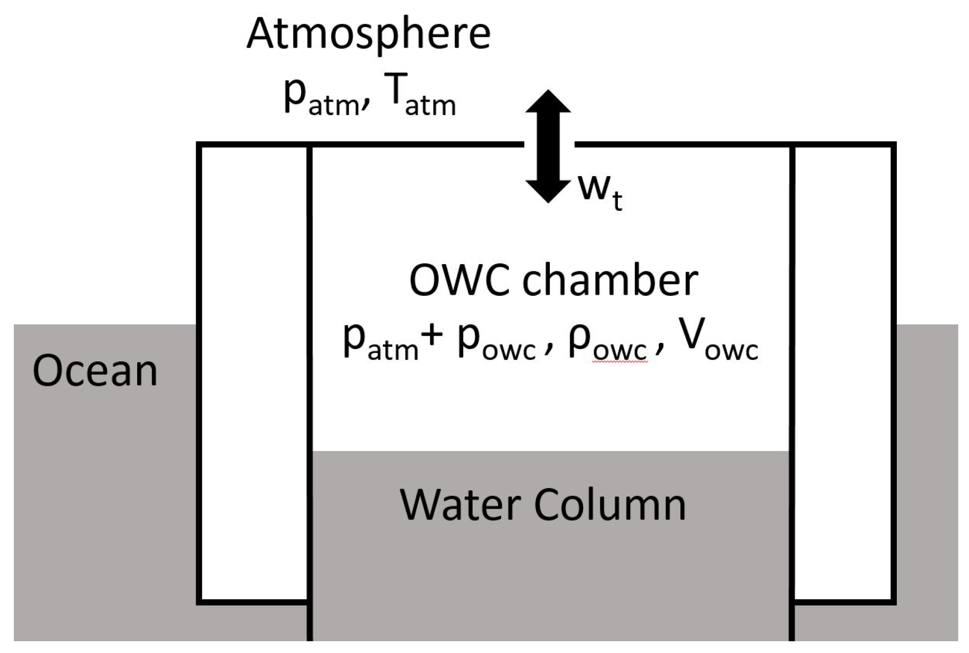
The air chamber in a conventional OWC device is commonly modelled in the literature using the linearized isentropic assumption. The main justification is that the temperature oscillations in the air chamber are relatively small and their time scales (a few seconds) are too short for significant heat exchanges to occur across the chamber walls and across the air-water interface [6]. It was proven in [25] that the linearised isentropic assumption provides a satisfactory results for the modelling of conventional OWCs except possibly under very rough sea conditions. In this paper, the numerical model will be compared to model-scale experimental results where pressure and temperature oscillations are even smaller. The use of the linearised isentropic assumption is hence justified. Figure 3 displays a schematic of the OWC thermodynamic system.

At model scale, the turbine (of impulse type) connecting the inside of the chamber to the atmosphere is modelled using an orifice plate. In the conventional OWC, the flow is bidirectional through the orifice. Hence, the density of the air entering the turbine is either ${\rho }_{atm}$ during the inhalation process ($p_{owc}<0$) or ${\rho }_{owc}$ during the exhalation process ($p_{owc}>0$). Under the testing conditions, the maximum excess pressures observed in the OWC chamber were $\pm 1250\mathrm{Pa}$, for which, according to Equation (8), ${\rho }_{owc}$ reaches the maximum values of ${\rho }_{atm}\pm 0.8\%$. Hence, the air in the OWC chamber can be considered as quasi-incompressible, and the air flow rates are described using the volumetric flow rates ([26,27]):

$$\Delta p=k_t{q}_t^2\mathrm{with}{k}_t={\displaystyle \frac{{\rho }_{atm}}{2{\left(\alpha A_t\right)}^2}}$$

(11)

where $q_t$ is the volumetric flow rate across the orifice/turbine, $k_t$ is the turbine damping coefficient, and $\alpha A_t$ is the effective area of the orifice representing the turbine.

Finally, according to Equations (10) and (11), the relationship between the hydrodynamic body motions (see Equation (1)) and the excess pressure in the OWC chamber is:

$${\dot{p}}_{owc}=\left\{\begin{array}{c}{\displaystyle \frac{\gamma p_{atm}}{{\rho }_{atm}{V}_{owc}}}\left(-{\rho }_{owc}\sqrt{{\displaystyle \frac{p_{owc}}{k_t}}}-{\rho }_{owc}{\dot{V}}_{owc}\right)\mathrm{for}{p}_{owc}>0\hfill \\ {\displaystyle \frac{\gamma p_{atm}}{{\rho }_{atm}{V}_{owc}}}\left(+{\rho }_{atm}\sqrt{{\displaystyle \frac{p_{owc}}{k_t}}}-{\rho }_{owc}{\dot{V}}_{owc}\right)\mathrm{for}{p}_{owc}<0\hfill \end{array}\right.$$

(12)

2.2.3. Tupperwave Device Thermodynamics

In the Tupperwave device, air is exchanged between three different air chambers. Unlike for the conventional OWC where the OWC chamber is open to the atmosphere, the air in the Tupperwave device is flowing in a closed-circuit. This raises the issue of a possible air temperature increase in the device due to heat created by viscous effects, mainly happening in the turbine. It was shown in [28] that the heat created is dissipated through the device walls, and only a slight temperature increase (<1 °C) is observed in moderate sea states.

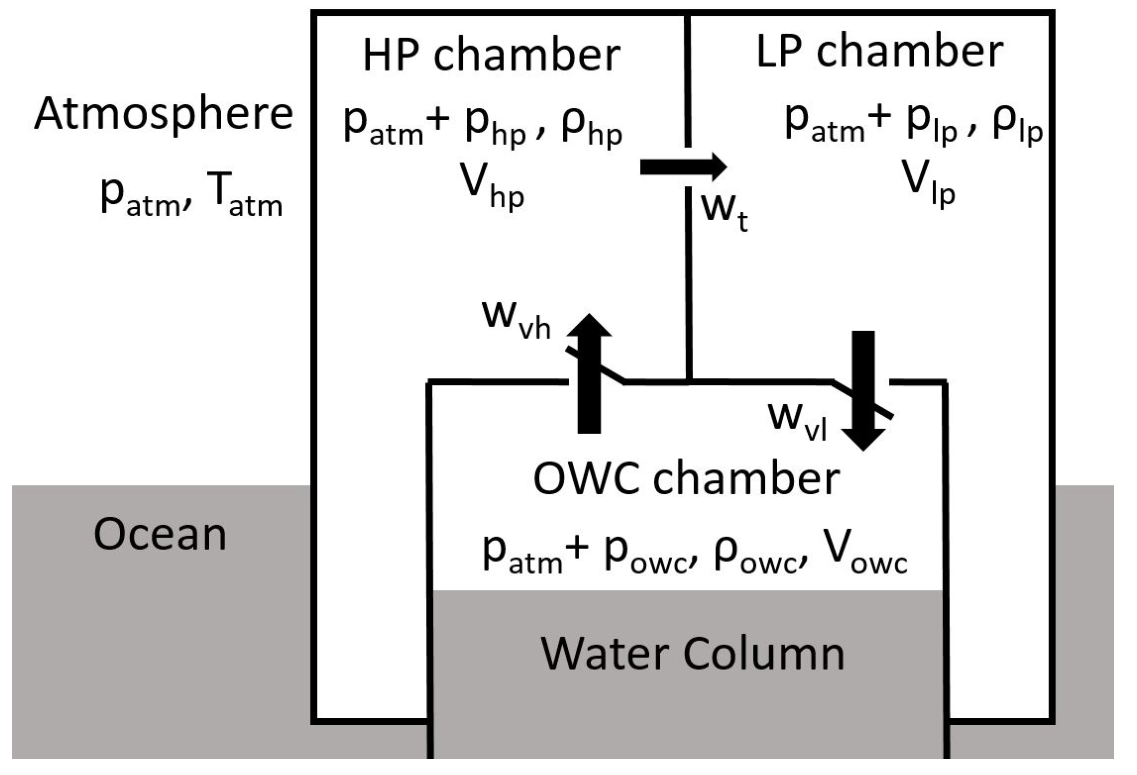
At model scale, the temperature increase is expected to be negligible. Moreover, the pressures reached in the device are expected to be in the same order as in the conventional OWC. Hence, the linearized isentropic assumption is assumed to be valid. Figure 4 displays a schematic of the three chambers, which constitute three interconnected thermodynamic systems.

Equation (10c) can be directly applied to the three chambers:

$$\left\{\begin{array}{c}{\dot{p}}_{owc}={\displaystyle \frac{\gamma p_{atm}}{{\rho }_{atm}{V}_{owc}}}(w_{vl}-w_{vh}-{\rho }_{owc}{\dot{V}}_{owc})\left(a\right)\hfill \\ {\dot{p}}_{hp}={\displaystyle \frac{\gamma p_{atm}}{{\rho }_{atm}{V}_{hp}}}(w_{vh}-w_t)\left(b\right)\hfill \\ {\dot{p}}_{lp}={\displaystyle \frac{\gamma p_{atm}}{{\rho }_{atm}{V}_{lp}}}(w_t-w_{vl})\left(c\right)\hfill \end{array}\right.$$

(13)

where $w_t$, $w_{vh}$, and $w_{vl}$ are the mass air flow rates across the turbine, the HP valve, and the LP valve. The sign convention for the volumetric flow rates is given by the arrow directions in Figure 4.

As for the conventional OWC, the excess pressures reached in the different chambers at model scale do not exceed $1250\mathrm{Pa}$. The variation of air density is therefore small, and the flow across the orifice is considered as incompressible:

$$w_t={\rho }_{hp}\sqrt{{\displaystyle \frac{p_{hp}-p_{lp}}{k_t}}}$$

(14)

The valves are non-return valves that close under a certain opening pressure $p_o$. When opened, their model is similar to orifice plates of effective opening area $\alpha A_v$ and damping coefficient $k_v={\displaystyle \frac{{\rho }_{atm}}{2{\left(\alpha A_v\right)}^2}}$:

$$w_{vh}=\left\{\begin{array}{c}0\mathrm{if}{p}_{owc}-p_{hp}<p_o\hfill \\ {\rho }_{owc}\sqrt{{\displaystyle \frac{p_{owc}-p_{hp}-p_o}{k_v}}}\mathrm{if}{p}_{owc}-p_{hp}>p_o\hfill \end{array}\right.$$

(15)

$$w_{vl}=\left\{\begin{array}{c}0\mathrm{if}{p}_{lp}-p_{owc}<p_o\hfill \\ {\rho }_{lp}\sqrt{{\displaystyle \frac{p_{lp}-p_{owc}-p_o}{k_v}}}\mathrm{if}{p}_{lp}-p_{owc}>p_o\hfill \end{array}\right.$$

(16)

The system of Equation (13a,b,c) is coupled with the hydrodynamic system of Equation (2a,b) and completes the model for the Tupperwave device.

2.3. Numerical Solution

The conventional OWC is governed by the coupled Equations (2a,b) and (12), while the Tupperwave device is governed by Equations (2a,b) and (13a,b,c).

The four convolution integrals $I_{ij}\left(t\right)={\int }_0^t{K}_{ij}(t-\tau ){\dot{x}}_j\left(\tau \right)d\tau$ present in Equation (2a,b) are called memory effect integrals. Their values depend on the history of the system, which implies their recalculation at each time step and is not practical for the system resolution. By using the conventional Prony methods [29], it is possible to calculate each of these functions as the sum of $N_p$ additional unknowns {$I_{ij,k}$, $k=1:N_p$}, which are the solutions of $N_p$ additional first order equations that will be solved along with the system of Equation (2a,b). Details on the conventional Prony method are given in Appendix A. Following the recommendations made in [30], $N_p=4$ was taken for the approximation of the impulse function of heave motion, which adds 16 first order equations to the system.

The solution of these equations was obtained numerically using the ordinary differential equation solver ode45 from the mathematical software MATLAB [31].

3. Physical Modelling in the Wave Tank

3.1. Physical Models Design and Fabrication

3.1.1. Scaling

The devices displayed in Figure 2 were built at model scale. For dynamic similarity in the water, all underwater dimensions were multiplied by the scaling factor $ϵ=0.0415\simeq 1/24$ according to the Froude similarity law. However, if the volumes of the high- and low-pressure chambers were also scaled using Froude scaling (i.e., multiplied by ${ϵ}^3$), air compressibility effects occurring at full scale would not be reproduced at model scale [32]. Since the Tupperwave device working principle fully relies on air compressibility in the high- and low-pressure chambers, these effects had to be reproduced, and a different scaling method was implemented for the volumes of the chambers.

As shown in Equation (13b), the variation of mass in the HP chamber of volume $V_{hp}$ is only due to air compressibility and directly related to the change in pressure:

$${\dot{p}}_{hp}={\displaystyle \frac{\gamma p_{atm}}{{\rho }_{atm}{V}_{hp}}}{\dot{m}}_{hp}$$

(17)

Equation (17) is valid both at full scale (F) and model scale (M). Hence:

$${\displaystyle \frac{{\dot{p}}_{hp,M}}{{\dot{p}}_{hp,F}}}={\displaystyle \frac{p_{atm,M}{\dot{m}}_{hp,M}{\rho }_{atm,F}{V}_{hp,F}}{p_{atm,F}{\dot{m}}_{hp,F}{\rho }_{atm,M}{V}_{hp,M}}}$$

(18)

For similitude to be achieved between full scale and model scale, Froude scaling laws need to be respected. This implies:

$$\left\{\begin{array}{c}{\displaystyle \frac{{\dot{p}}_{hp,M}}{{\dot{p}}_{hp,F}}}={ϵ}^{1/2}\hfill \\ {\displaystyle \frac{{\dot{m}}_{hp,M}}{{\dot{m}}_{hp,F}}}={ϵ}^{5/2}\hfill \end{array}\right.$$

(19)

Unless very specific infrastructures are used, the atmospheric conditions are the same at model scale as at full scale, hence:

$$\left\{\begin{array}{c}{p}_{atm,M}=p_{atm,F}\hfill \\ {\rho }_{atm,M}={\rho }_{atm,F}\hfill \end{array}\right.$$

(20)

Combining Equation (18) with Equations (19) and (20) leads to the necessary condition on the chamber volume to satisfy similarity regarding compressibility effects between full scale and model scale:

$${\displaystyle \frac{V_{hp,M}}{V_{hp,F}}}={ϵ}^2$$

(21)

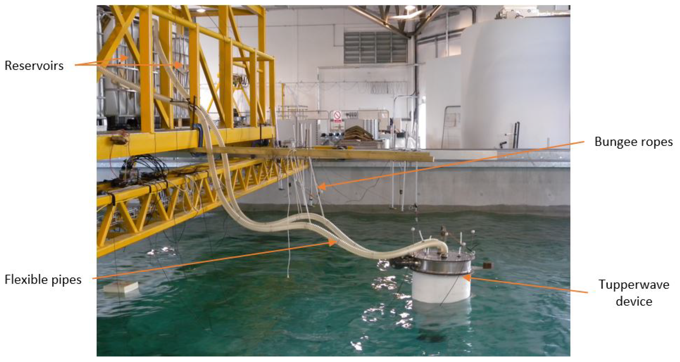
The same condition needs to be satisfied for the LP chamber. At full scale, the HP and LP chamber are $950{\mathrm{m}}^3$. At model scale, the volumes of the chambers therefore are $1.64{\mathrm{m}}^3$. Unlike full scale, it is impossible to fit both chambers on the device as their volume largely exceeds the overall volume of the device. The alternative at small scale is to locate the main volume of the HP and LP chambers outside of the device and connect them to two smaller chambers on the device with flexible pipes. Large reservoirs were used for the HP and LP chambers and located on the pedestrian bridge above the tank, see Figure 5. The flexible pipes were chosen as lightweight and flexible as possible to reduce their influence on the floating device motion. Part of the pipes’ weight was supported by bungee ropes. A similar experimental setup was implemented in [33] to test a floating air bag wave energy converter at model scale.

This scaling method was suggested and applied in [32] to represent the spring-like effect of the air in the OWC chamber of a conventional OWC device properly. To implement this method, an additional flexible pipe connecting the OWC chamber to another reservoir outside of the device is required. It is however rarely implemented at model scale by conventional OWC developers since the air compressibility in the OWC chamber is not essential for the devices working principle, and it increases even more the testing difficulty, especially for a floating device. Therefore, in the present experiments, the volume of the OWC chamber was simply scaled down by the factor ${ϵ}^3$ using direct Froude scaling, and the spring-like effect of the air in the OWC chamber was not physically modelled in both devices. The air in the OWC chamber is therefore quasi-incompressible in the conditions of the tests, and it is acknowledged that the perfect similitude with the full-scale devices is not achieved. The power conversion performances of the full scale devices can therefore not be directly obtained from the results of the model tests, as this may result in unrealistic overestimations [34]. The present experiments are however still valuable to validate the Tupperwave concept and compare it to the conventional OWC.

Since both devices use the same Spar structure, a single spar was built and used for both device. The schematics of the physical models are shown in Figure 6. The positions of the centre of gravity and centre of buoyancy, as well as the moments of inertia were assessed using the computer-aided design software Solidworks [35]. The position of the centre of gravity was also assessed experimentally by hanging the device on a vertical rope and finding the balance point. The values obtained experimentally after five repeated tests verified the centre of gravity to be within $\pm 1\mathrm{mm}$ from the position indicated by Solidworks. The moment of inertia around the horizontal axis Y parallel to the wave front was also verified using the bifilar pendulum method, and the values obtained were within $\pm 0.1\mathrm{kg}·{\mathrm{m}}^2$ from the value indicated by Solidworks. The conventional OWC being initially lighter than the Tupperwave device, it was ballasted such that both devices had the exact same mass properties. The mass properties of the device are given in

Table 1. Devices mass properties.

	Model Scale	Full Scale
Total mass (kg)	58.4	$817\times {10}^3$
Distance device bottom, COG(m)	0.892	21.49
Distance device bottom, COB(m)	0.961	23.16
Ixx ($\mathbf{kg}·{\mathbf{m}}^{\mathbf{2}}$)	23	$1.87\times {10}^8$
Iyy ($\mathbf{kg}·{\mathbf{m}}^{\mathbf{2}}$)	23.5	$1.91\times {10}^8$
Izz ($\mathbf{kg}·{\mathbf{m}}^{\mathbf{2}}$)	2	$1.62\times {10}^7$

.

3.1.2. Turbines

As mentioned in Section 2.2.2, the turbines were physically modelled using orifice plates. Preliminary numerical modelling showed that the optimal damping coefficients at full scale to maximise the pneumatic power output were close to $38\mathrm{Pa}·{\mathrm{s}}^2·{\mathrm{m}}^{-6}$ for the conventional OWC and $450\mathrm{Pa}·{\mathrm{s}}^2·{\mathrm{m}}^{-6}$ for the Tupperwave device [9]. Three orifice plates per device were built around those values scaled down using Froude scaling. Their exact damping coefficients and effective areas were then experimentally assessed prior to testing by forcing a known flow across the orifice and measuring the pressure drop [36].

Table 2. Orifice characteristics for the conventional OWC and Tupperwave device.

	Model Scale			Full Scale
Orifice	Diameter (mm)	${\mathbf{k}}_{\mathbf{t}}$ ($\mathbf{Pa}·{\mathbf{s}}^{\mathbf{2}}·{\mathbf{m}}^{-\mathbf{6}}$)	$\alpha \mathbf{A}$ (${\mathbf{m}}^{\mathbf{2}}$)	${\mathbf{k}}_{\mathbf{t}}$ ($\mathbf{Pa}·{\mathbf{s}}^{\mathbf{2}}·{\mathbf{m}}^{-\mathbf{6}}$)	$\alpha \mathbf{A}$ (${\mathbf{m}}^{\mathbf{2}}$)
OWC1	22.6	$7.10\times {10}^6$	$2.94\times {10}^{-4}$	21.1	$1.71\times {10}^{-1}$
OWC2	20.6	$10.4\times {10}^6$	$2.42\times {10}^{-4}$	30.9	$1.41\times {10}^{-1}$
OWC3	17.5	$19.6\times {10}^6$	$1.77\times {10}^{-4}$	58.3	$1.03\times {10}^{-1}$
T1	11.5	$0.70\times {10}^8$	$9.33\times {10}^{-5}$	209	$5.42\times {10}^{-2}$
T2	9.2	$1.86\times {10}^8$	$5.74\times {10}^{-5}$	552	$3.33\times {10}^{-2}$
T3	7	$4.85\times {10}^8$	$3.55\times {10}^{-5}$	1439	$2.06\times {10}^{-2}$

displays the orifice characteristics for the conventional OWC and the Tupperwave model scale devices. The damping coefficients were used during the tank testing to calculate the instantaneous volumetric flow across the orifice based on the measurement of the pressure drop according to Equation (14).

3.1.3. Valves

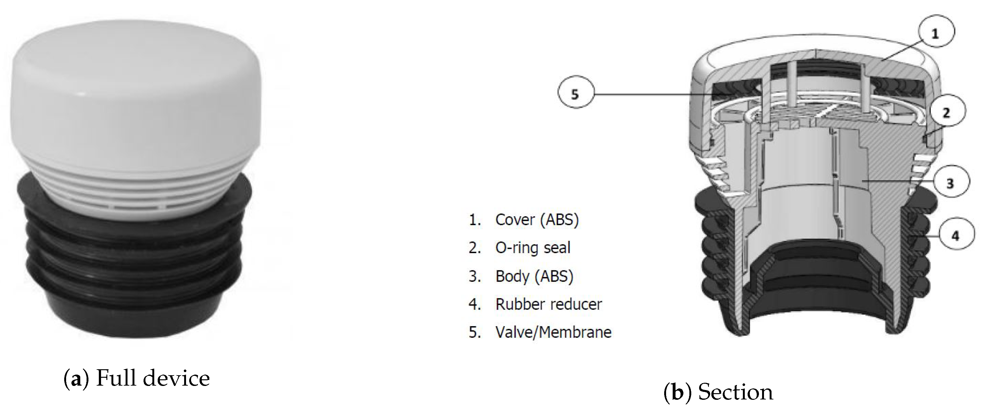
The Tupperwave working principle relies on the use of non-return valves. The valves are key components because they are likely to cause pneumatic power losses. They can either be passive or active. Passive valves mechanically open when a certain pressure difference is reached across the valves, while active valves are electrically activated. For the physical model, passive valves were chosen for their simplicity. The most appropriate valves found on the market were the Capricorn MiniHab HypAirBalance, see Figure 7.

They were passive normally closed air admittance valves from the plumbing market. A rubber membrane contained in the valve obstructs the opening of the valve due to gravity. When sufficient pressure is applied, the rubber membrane is lifted up, and the valve opens. Their opening pressure is 70 Pa (equivalent to 1686 Pa at full scale), and their light weight allowed their use in the small-scale Tupperwave physical model.

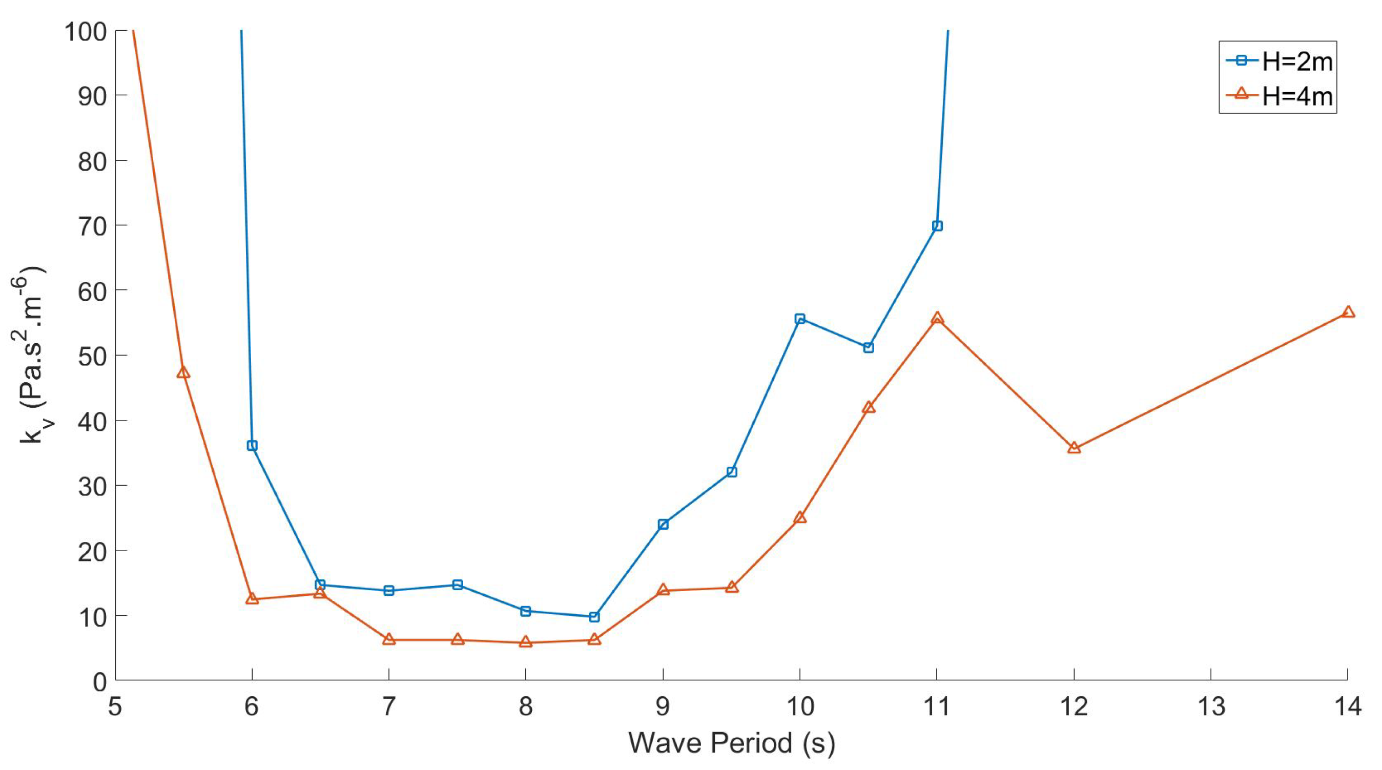
According to Equations (15) and (16), lower values of the valve damping coefficient $k_v$ reduce the pressure drop across the valves and hence reduce the pneumatic power losses. The value of $k_v$ is therefore fundamental for the device efficiency. Unlike for the orifices, the damping coefficient of the valves were experimentally assessed during each test by using Equations (15) and (16) and monitoring the pressure drop and air flow across the valves. The air flow rate across the valves was calculated from the measurement of the IWS elevation achieved with wave probes located inside the water column. Different valve damping values were obtained depending on the tests undertaken. Figure 8 displays the values of $k_v$ for the HP valve obtained in regular waves.

Wave height, wave period, and valve damping coefficients are given at full-scale equivalent. Variations of $k_v$ with the wave height and wave period were observed. It was shown in [38] that the damping coefficient of those valves is highly dependant on the device excitation. Indeed, when the device is well excited (for $6.5\mathrm{s}<T<8.5\mathrm{s}$), large pressure drops and flows across the valves are created. The valves therefore open fully, and their damping coefficient is small (large effective area). The lowest damping values reached by the valves were around $k_v=7.5\mathrm{Pa}·{\mathrm{s}}^2·{\mathrm{m}}^{-6}$ at full-scale equivalent, which corresponds to an effective valve opening area of $0.286{\mathrm{m}}^2$. This maximum opening area achieved was very small compared to the available $10.6{\mathrm{m}}^2$ between the OWC chamber and the HP chamber. When the device is poorly excited (for $T<6.5\mathrm{s}$ and $T>8.5\mathrm{s}$), the valves do not open fully and create large damping (i.e., large losses). For $H=4\mathrm{m}$, the valves open fully on a larger range of wave periods than for $H=2\mathrm{m}$ since the device is more excited in bigger waves. The values of the valves’ damping coefficient assessed for each regular wave physical test were fed into the numerical model for the corresponding numerical test.

In irregular waves, the excitation of the device varies with the incoming wave groups. Hence, the instantaneous damping of the valves fluctuates along the simulation. The $k_v$ values in-putted in the numerical model for each irregular wave simulations were the average damping values obtained physically over the whole duration of the simulations.

3.2. Experimental Setup and Test Plan

The experiments took place in the Lir-National Ocean Test Facility (Lir-NOTF) of the MaREIcentre in Cork, Ireland. The devices were tested under regular and irregular sea states in the Deep Ocean Basin, which is $35\mathrm{m}$ long, $12\mathrm{m}$ wide, and has a movable floor with up to $3\mathrm{m}$ of depth. For the regular sea states and at full-scale equivalent, 2 wave heights (2 m and 4 m) were tested with periods ranging from 5–14 s. A set of 8 irregular sea states of various significant wave heights (2–5 m) and peak periods (5–14 s) was also tested. These sea states were chosen to represent a large variety of typical conditions in the Atlantic Ocean. The depth was set to $2.07\mathrm{m}$, equivalent to $50\mathrm{m}$ at full scale.

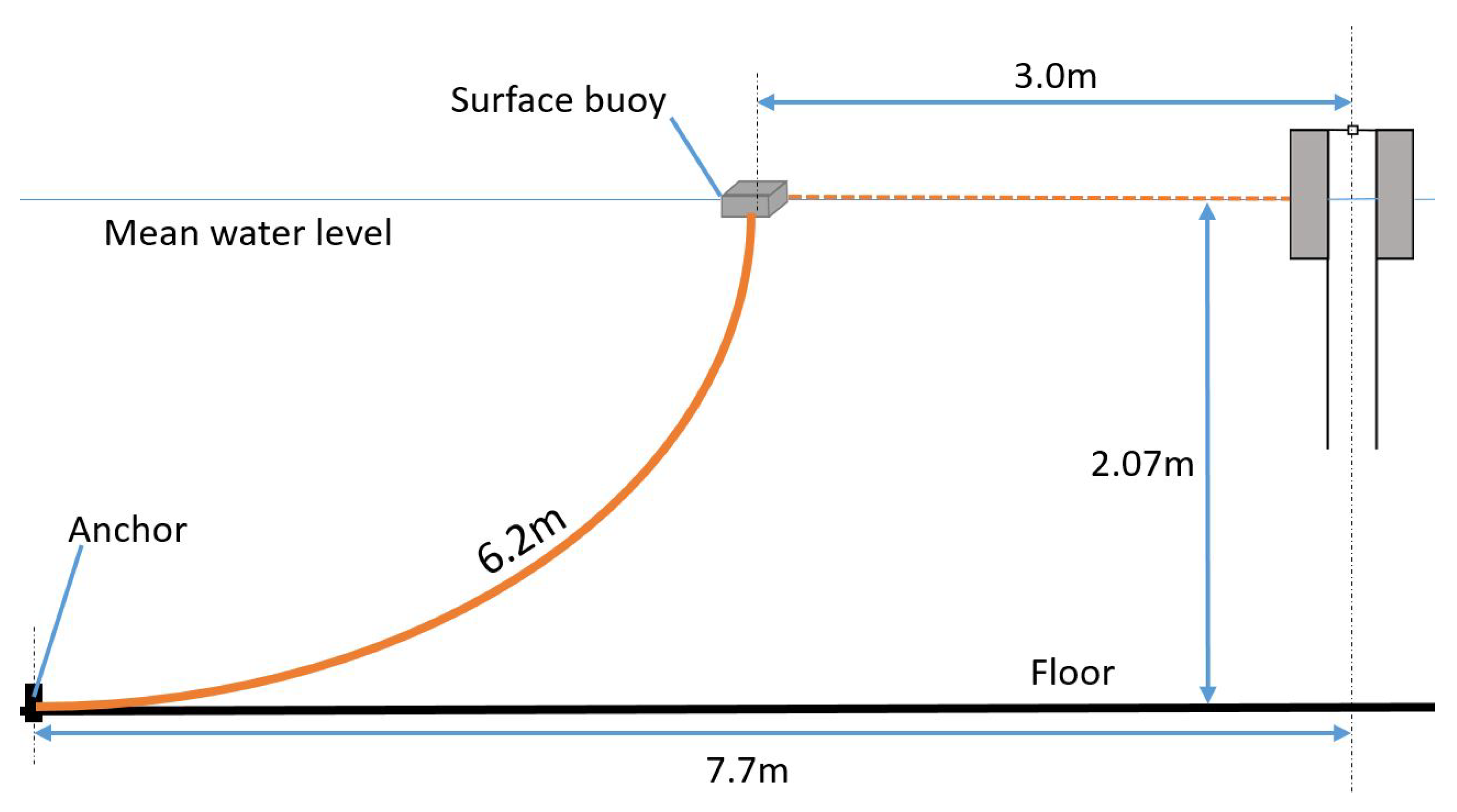
The devices were moored using a 3-point mooring arrangement of the catenary type with 120 degrees between any two mooring lines. There were two bow mooring lines and one stern line. Each line was divided into two parts: a steel chain connects the anchor to a surface buoy that can support the chain weight. A neutrally-buoyant line then connects the surface buoy to the device at the mean water level. Figure 9 shows a schematic of one mooring line. With such a mooring configuration, the mooring forces applied on the device were principally horizontal, preventing the device from drifting in the waves, with a minimum impact on the heave motion from which the wave energy was absorbed. Therefore, the vertical component of the mooring force applied on the device was neglected in the numerical model presented in Section 2. The drag forces caused by the vertical motion of the neutrally buoyant lines with the device were taken into account in the numerical model by the equivalent drag coefficient $C_d$.

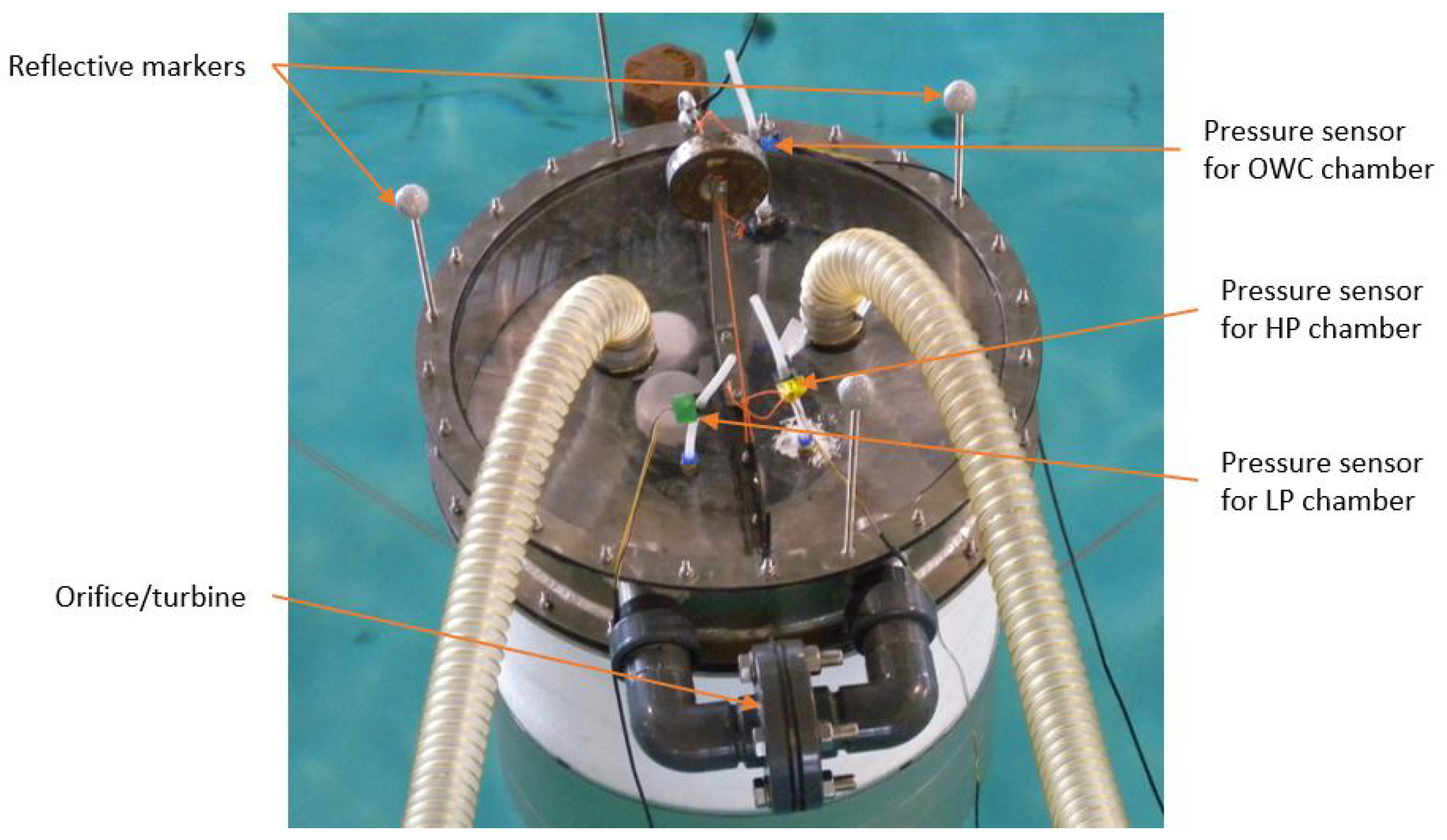
The devices were fully monitored using 3D cameras, pressure sensors, and wave probes, allowing the measurement of the devices’ motions, IWS elevation, pressure drops, and volumetric flow rates across orifices and valves. Wave probes located outside of the device measured the incoming wave elevation. A wave probe located inside the column of the device measured the relative elevation of the water column relative to the buoy. Figure 10 displays a picture of the device, from above, equipped with pressure sensors and reflective markers for the 3D cameras.

The power absorbed from the waves by the devices is the power applied by internal water surface (IWS) on the air contained in the OWC chamber and was calculated, from those measurements, as:

$$P_{abs}=p_{owc}.\dot{V}=p_{owc}{S}_2\frac{d{x}_{IWS}}{dt}$$

(22)

where $x_{IWS}=x_2-x_1$ is the position of the IWS relative to the buoy. In testing conditions, the flows across the orifice or valves were incompressible. The pneumatic power available to the turbine $P_t$ or to a valve $P_v$ was therefore calculated as the product of the volumetric flow and the pressure drop:

$$P=\Delta pq$$

(23)

The regular wave tests were 125 s long, which is equivalent to 10 min at full scale. The irregular wave tests were 7 min long, which is equivalent to 35 min at full scale. This allows a full representation of the Bretschneider sea state.

For the analysis of regular wave tests, averaging of the key variables was made over several waves once a steady state was reached, practically between 90 and 115 s at model scale. The average values in irregular sea states were calculated over the full time of the simulation.

4. Results and Numerical Model Validation

Physical and numerical tests were carried out for the small-scale devices, but all results were given in full-scale equivalence to give the reader perspective.

4.1. Correction in the Tupperwave Numerical Model

During the tests, it was observed that the reservoirs used for the HP and LP chambers of the Tupperwave physical model did not have perfectly rigid walls and that the walls moved very slightly due to the pressure building inside the chambers. The HP chamber was observed to inflate with the build-up of a positive excess pressure inside, and the LP chamber was observed to deflate due to the negative excess pressure inside. Unfortunately, within the time frame and budget of the project, it was not possible to replace the chamber walls with stiffer material. As a result, the air compressibility in the HP and LP chambers was physically not modelled correctly, and the varying volumes of the chambers caused a dampening of the pressure variations. This required a correction in the initial numerical model described in Section 2.2.3 to take into account the slight volumetric changes of the HP and LP chambers.

A simple linear model of the chamber volumetric deformation as a function of the excess pressure was chosen:

$$\left\{\begin{array}{c}{V}_{hp}=V_0+C{p}_{hp}\hfill \\ V_{lp}=V_0+C{p}_{lp}\hfill \end{array}\right.$$

(24)

where C is the elastic stiffness of the chambers and $V_0=1.64{\mathrm{m}}^3$ is their initial volume.

The same stiffness value was applied to the two chambers, and its value was calibrated using the experimental results. The value $C=8.3\times {10}^{-5}{\mathrm{m}}^3·{\mathrm{Pa}}^{-1}$ was obtained by an iterative process to minimise the error with the experimental results in the different irregular sea states. Therefore, for an excess pressure of $p_{ref}=\pm 1000\mathrm{Pa}$ (close to maximum pressure observed in the chambers), the volume variations of the chamber were $d{V}_{ref=}\pm 0.083{\mathrm{m}}^3<<V_0$, which is equivalent to a $\pm 2\mathrm{cm}$ deformation of the edge lengths of the cubic chambers and corresponds to the approximate visual observations.

The system of Equation (13) describing the pressure evolution in the Tupperwave chambers was modified to take into account the HP and LP chambers deformations:

$$\left\{\begin{array}{c}{\dot{p}}_{owc}={\displaystyle \frac{\gamma p_{atm}}{{\rho }_{atm}{V}_{owc}}}(w_{vl}-w_{vh}-{\rho }_{owc}{\dot{V}}_{owc})\left(a\right)\hfill \\ {\dot{p}}_{hp}={\displaystyle \frac{\gamma p_{atm}}{{\rho }_{atm}{V}_{hp}}}(w_{vh}-w_t-{\rho }_{hp}{\dot{V}}_{hp})\left(b\right)\hfill \\ {\dot{p}}_{lp}={\displaystyle \frac{\gamma p_{atm}}{{\rho }_{atm}{V}_{lp}}}(w_t-w_{vl}-{\rho }_{lp}{\dot{V}}_{lp})\left(c\right)\hfill \end{array}\right.$$

(25)

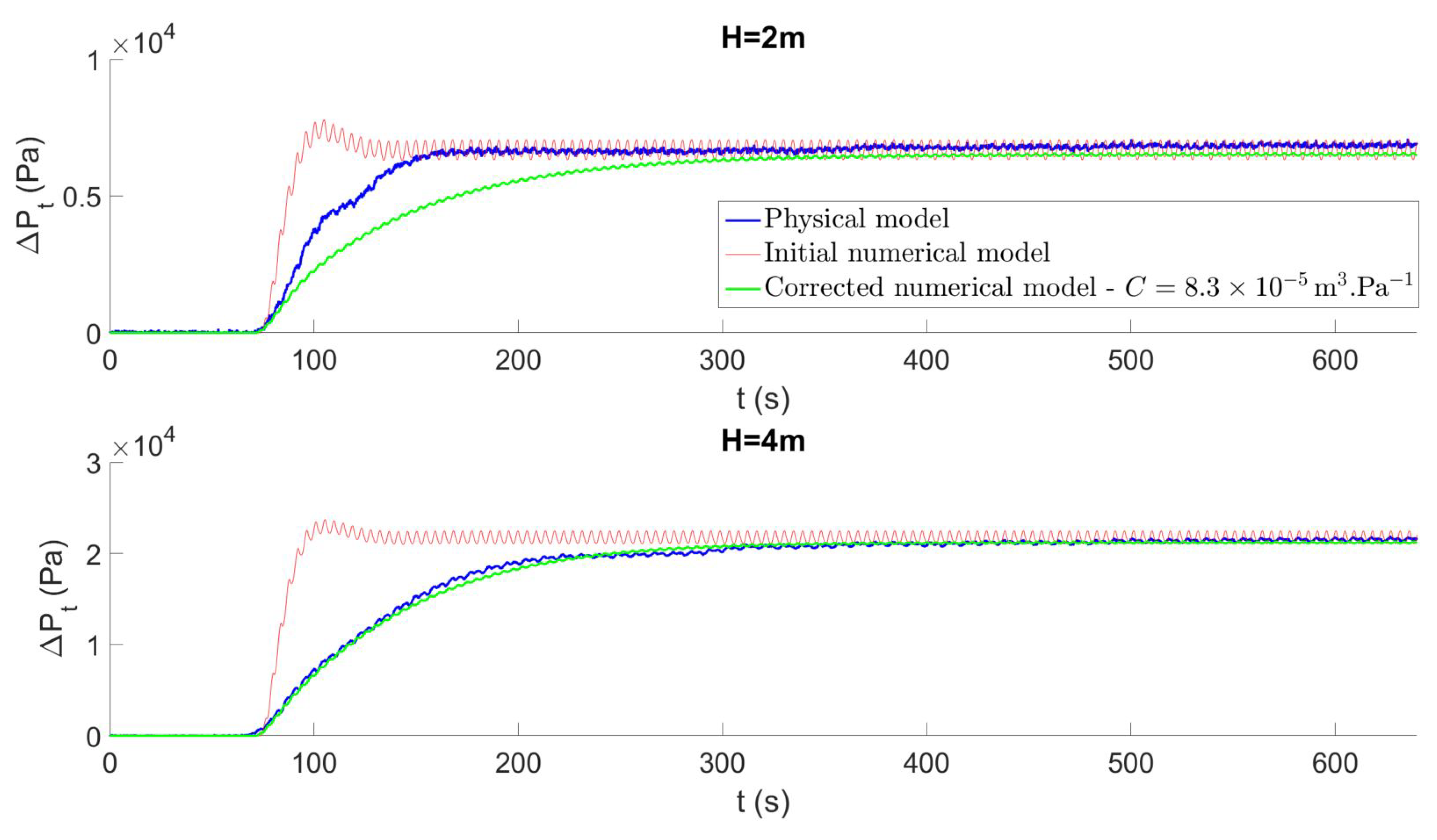
Figure 11 compares the time series of the pressure drop $\Delta P_t=p_{hp}-p_{lp}$ across the orifice of the Tupperwave device in regular waves of a 9-s period and heights of $2\mathrm{m}$ and $4\mathrm{m}$ obtained by the physical model, the initial numerical model, and the corrected model. In regular waves, the wave excitation on the device is steady, and the excess pressures in the HP and LP chambers increased until they stabilized to certain values and reached a steady state. In the initial numerical model where the HP and LP chambers were perfectly rigid, the pressure drop between the chambers built up quickly to reach the steady state. Small pressure drop oscillations with a period of half a wave period were also visible and were due to the oscillatory motion of the water column. In the physical model, the chambers deformed gradually by a corresponding small volume $\pm \Delta V,$ much less than the initial volume $V_0$, and consequently delayed the pressure evolution. Hence, the slight deformation of the chambers did not influence the end results in regular waves, but simply delayed the system from reaching steady state. The smaller oscillations were also attenuated.

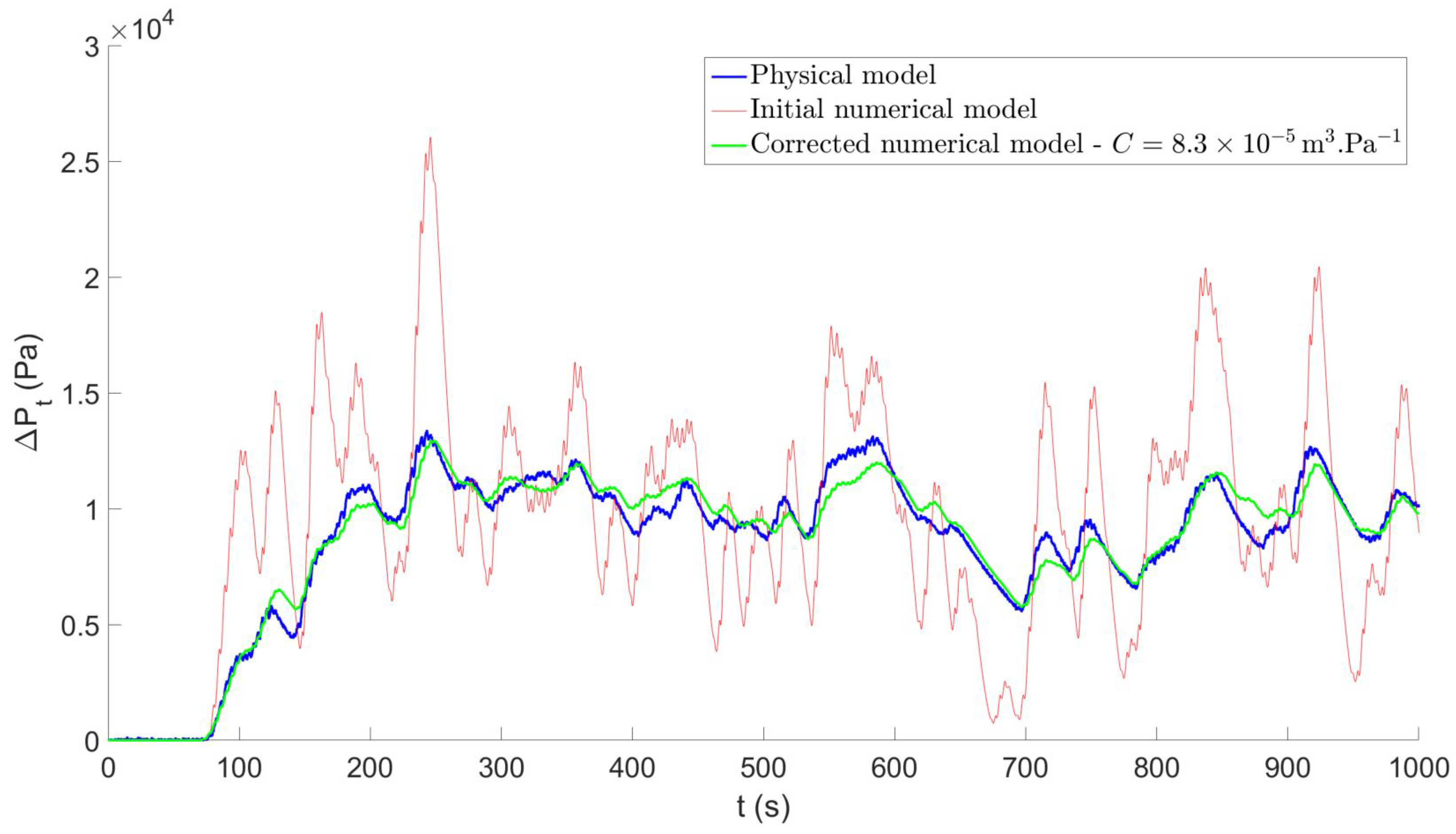
In irregular waves, however, the slight volumetric deformations of the chambers caused more visible effects. During a simulation, the pressures in the HP and LP chambers varied significantly when the device was excited by high or low energy wave groups. The chamber volumes were therefore changing between wave groups and dampened fast pressure variations. Figure 12 compares the time series $\Delta P_t$ in the irregular sea state {$H_s=3$ m; $T_p=8.5$ s} obtained physically against the time series obtained with the initial and corrected numerical model. The pressures in the rigid-wall chambers from the initial numerical model varied more rapidly with the wave groups than in the chambers used in the physical tests. As a result of the chambers’ deformation, an extra and unrealistic smoothing effect of the pressure variations between the wave groups was observed in irregular waves. Accounting for the small volume variations of the HP and LP chambers in the numerical model very clearly enhanced the fidelity of the physical model.

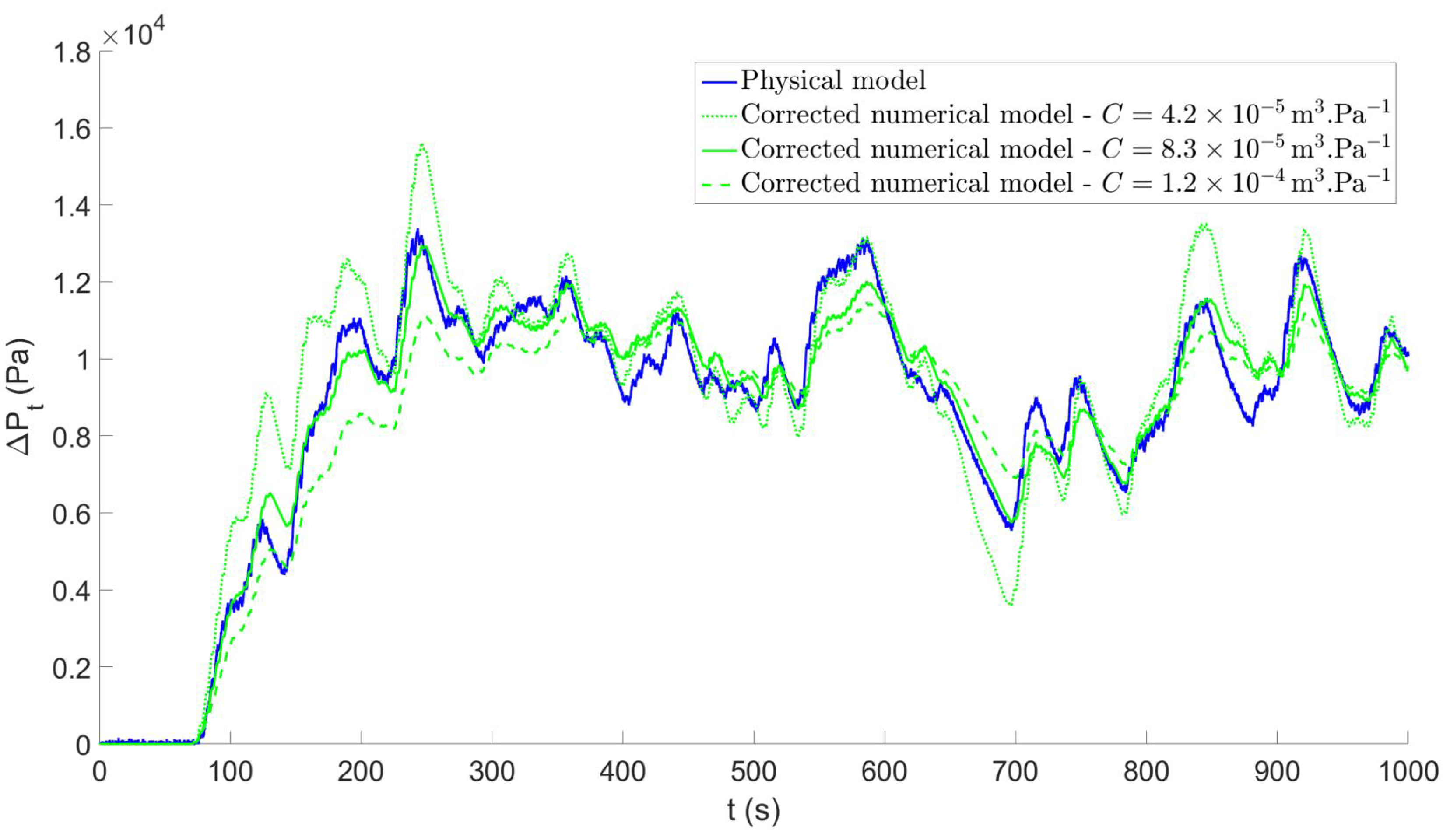
Figure 13 displays the numerical results obtained with the following chamber stiffness values: $[4.2;8.3;12]\times {10}^{-5}{\mathrm{m}}^3·{\mathrm{Pa}}^{-1}$, corresponding respectively to $\pm [1;2;3]$ cm deformation of the chambers’ edge length for an excess pressure of $p_{ref}=\pm 1000\mathrm{Pa}$. This figure shows the sensitivity of the results on the chambers’ stiffness value. With stiffer chambers ($C=4.2\times {10}^{-5}{\mathrm{m}}^3·{\mathrm{Pa}}^{-1}$), the pressure variation was larger due to the smaller deformation of the walls. The pressure variations were more dampened with more flexible chambers ($C=1.2\times {10}^{-4}{\mathrm{m}}^3·{\mathrm{Pa}}^{-1}$). Although the results were not extremely sensitive on the stiffness value, $C=8.3\times {10}^{-5}{\mathrm{m}}^3·{\mathrm{Pa}}^{-1}$ obtained the closest results to the physical model for all sea states tested.

Table 3. Pearson correlation coefficient between $\Delta P_t$ time series obtained physically and numerically for the various irregular sea states.

Sea State		Pearson Correlation Coefficient (-)
${\mathit{H}}_{\mathit{s}}$ (m)	${\mathit{T}}_{\mathit{p}}$ (s)	Initial Model	Corrected Model $\mathit{C}=\mathbf{8}.\mathbf{3}\times {\mathbf{10}}^{-\mathbf{5}}{\mathrm{m}}^3·{\mathrm{Pa}}^{-1}$
2	5.7	0.72	0.85
3	7.1	0.68	0.93
3	8.5	0.69	0.93
5	8.5	0.65	0.94
3	10.6	0.70	0.94
5	10.6	0.65	0.93
5	12.7	0.62	0.93
3	14.1	0.70	0.86

displays the Pearson correlation coefficients between the time series obtained physically and the time series obtained with the initial and corrected numerical models. Values closer to one indicate a better correlation between physical and numerical results.

From an energy point of view, the pneumatic energy stored in the HP and LP chamber was not only stored in the form of pressure, but also under the form of strain energy. This explains the lower pressure variations between wave groups, and the average value of the pressure drop across the orifice was not impacted; see Figure 12. In the next section, only the corrected numerical model of the model-scale device accounting for the chambers’ deformation was used.

We note that the idea of storing pneumatic energy under the form of strain energy could be combined with the Tupperwave concept at full scale, by adding a spring and piston to the HP and LP chambers for example. This would enable further improving the pneumatic power smoothing capacity of the device or reducing the volumes of the reservoirs. Moreover, this would possibly introduce further control possibilities: changing the stiffness of the spring could enable the device to be tuned to the sea state to improve energy extraction (or de-tuned if desired). The concept variation of the Tupperwave device using variable volume HP and LP chambers will be investigated in further work and is not in the scope of this paper. With fixed volume chambers, the Tupperwave device was structurally and mechanically simple. History has shown that mechanical simplicity represents an advantage in the development of wave energy devices, particularly regarding the device cost, maintainability, and reliability. Developers commonly claim the simplicity of their wave energy device as an advantage [39,40,41].

4.2. Numerical Model Validation

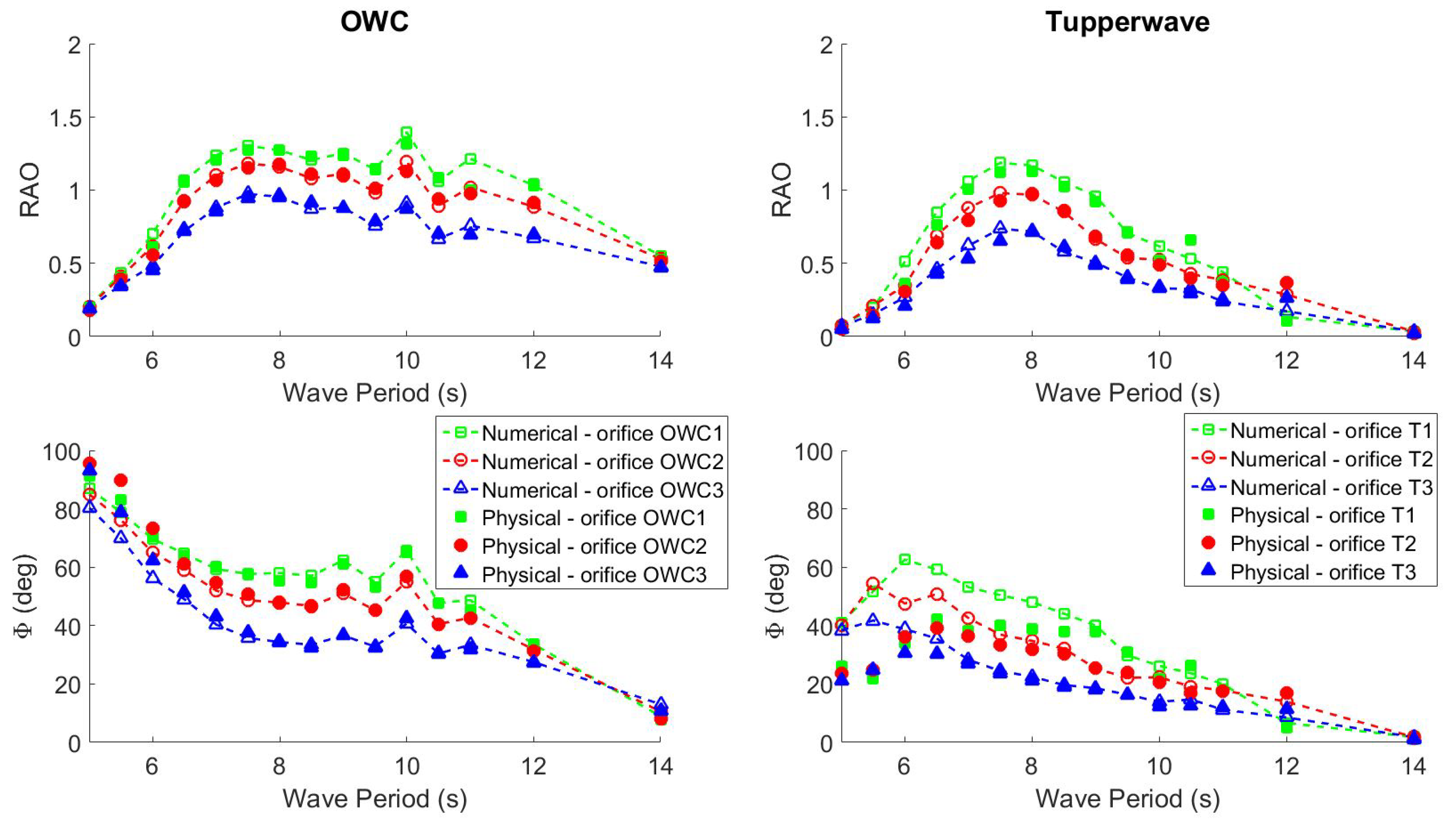
For the validation process, the spar buoy and water column relative motions were first compared in regular waves. Figure 14 displays the Response Amplitude Operator (RAO) of the bodies’ relative sinusoidal heave oscillations and their phase difference for the two devices. The numerical models agree generally well with the results obtained by the physical tests, and the influence of the different orifice damping tested is well predicted. The phase difference between the bodies in the Tupperwave device for short wave period was less accurately predicted by the numerical model than for the conventional OWC. It is interesting to note that, for the two devices, smaller orifices restricted both the relative motion amplitude and the phase difference between the bodies. In the conventional OWC, the larger damping of small orifices directly caused more resistance against the bodies’ relative motions. In the Tupperwave device, the larger damping of small orifices created larger excess pressures in the HP and LP chamber, which increased the necessary OWC chamber pressure to open the valves and thus caused more resistance against the bodies’ relative motions.

Furthermore, in comparison to the conventional OWC, the response of relative motion amplitude in the Tupperwave device was narrower, and the phase difference between the bodies was lower. This shows that the coupling between the structure and the water column was stiffer, and the bodies were more constrained to oscillate together in the Tupperwave device.

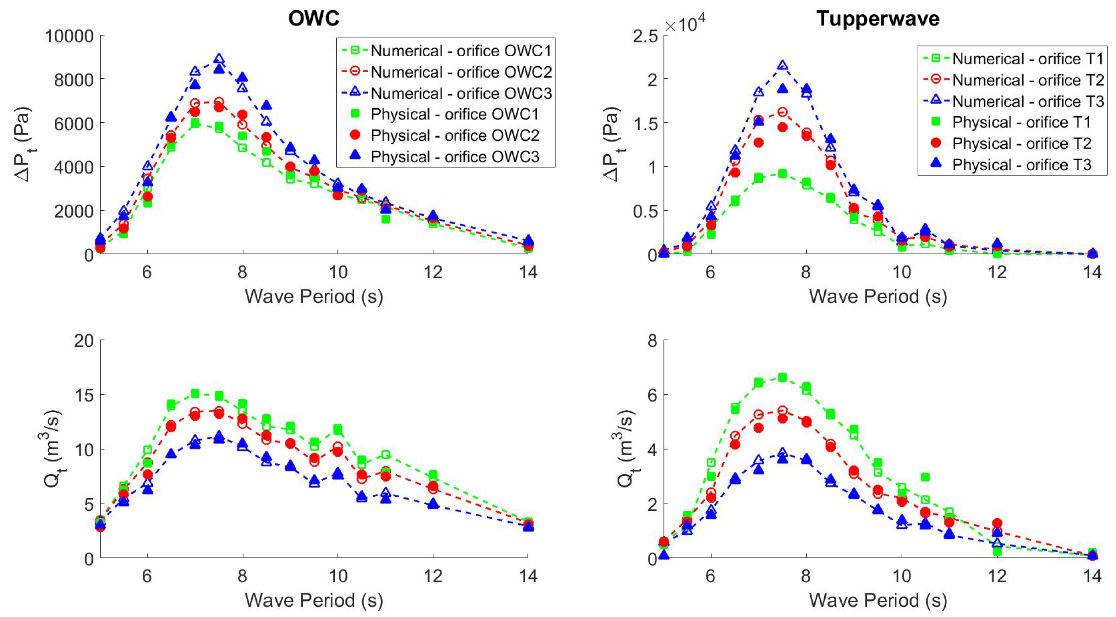
The average pressure drop and volumetric flow across the orifices in regular waves are compared in Figure 15. Good agreement was obtained between numerical and physical results. In both devices, the pressure drop decreased with increasing orifice diameter, and the flow across the orifice increased. The Tupperwave device produced larger pressure drops and lower flow rates across the turbine than the conventional OWC.

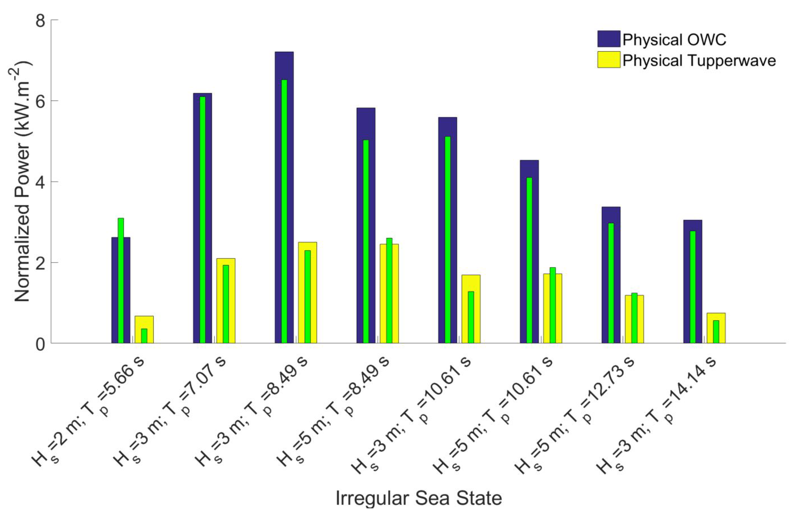
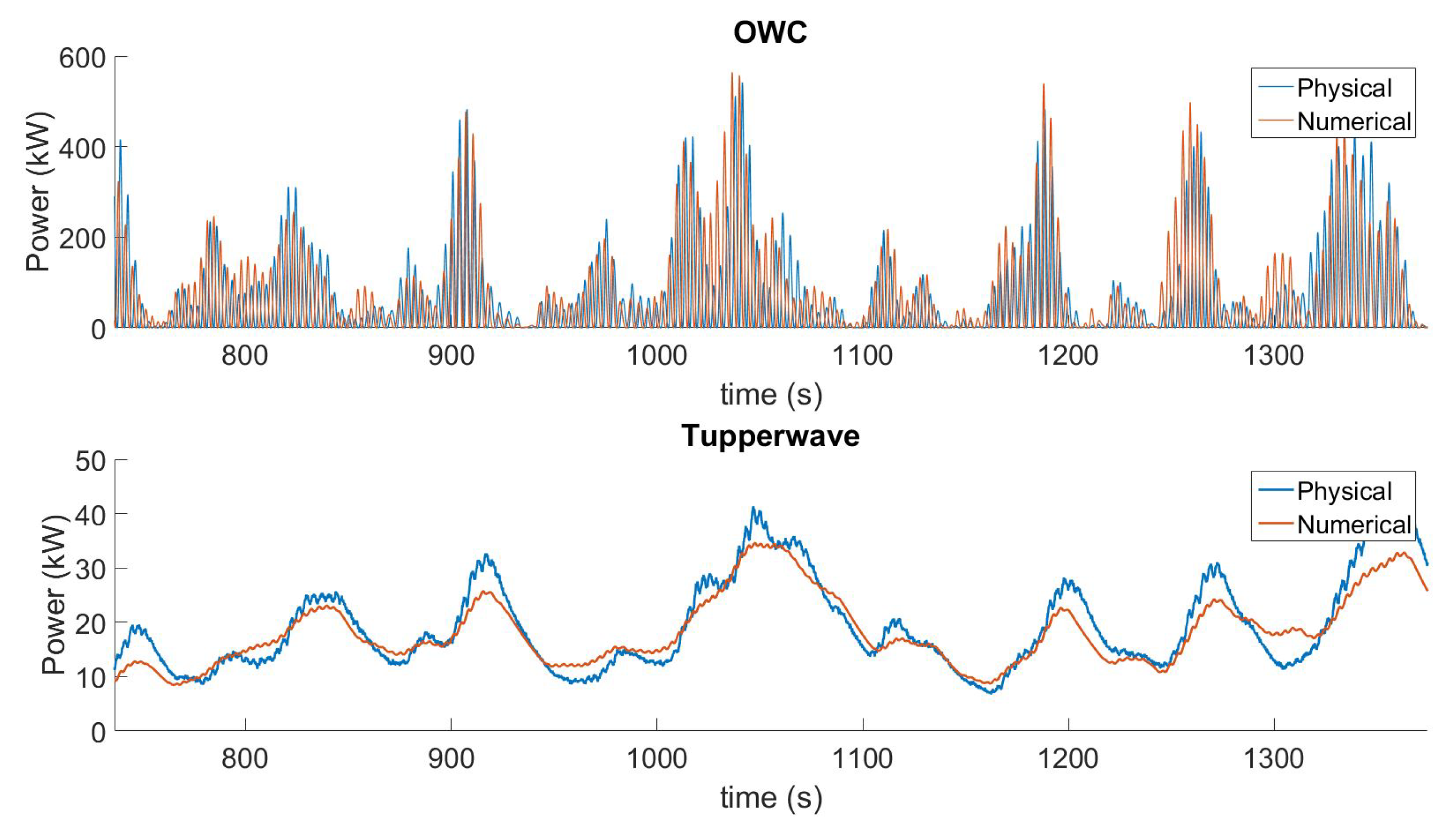
Figure 16 displays the average pneumatic power normalized by the significant wave height squared obtained numerically and physically by the two devices in the eight irregular sea states tested. Figure 17 displays the time series of the pneumatic power for the irregular sea state {$H_s=3$ m; $T_p=7.1$ s}. The two devices were equipped with their most efficient orifices (OWC2 and T2).

Good overall agreement was obtained between physical and numerical results. The errors of the numerical models on average power prediction in irregular wave tests in Figure 16 were 10.1% for the conventional OWC and 16.5% for the Tupperwave device. The passive valves in the Tupperwave model are an additional component to model, and their fluctuating behaviour with the device excitation in irregular waves (see Section 3.1.3) is hence an additional source of error in numerical model fidelity.

Although moderate pitch and roll motions of the spar buoy were observed during the experiments, the satisfactory results of the numerical model prove, a posteriori, that considering heave only in the numerical model is a reasonable approach to assess the devices’ power conversion.

4.3. Power Performance Comparison

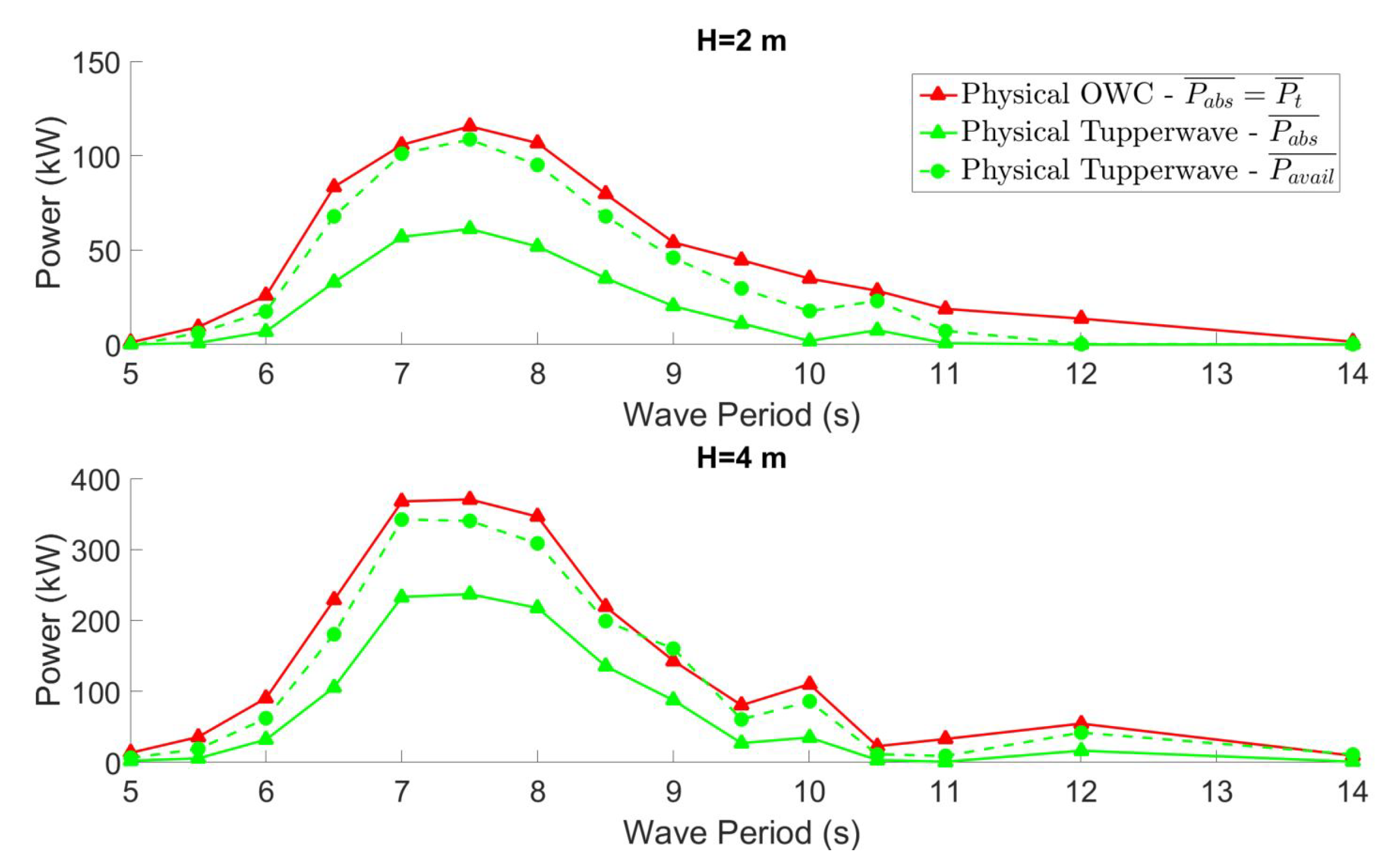
Figure 18 displays the average power absorbed by the device from the waves $\overline{P_{abs}}$ and the average pneumatic power $\overline{P_{avail}}$ available to the turbine in both devices in 2 and 4 m-high regular waves. In the case of the conventional OWC, the absorbed power is, on average, entirely made available to the turbine $\overline{P_{abs}}=\overline{P_{avail}}$ [34]. The Tupperwave device absorbed 4–20% less power from the waves than the conventional OWC for wave periods between 6 and 9.5 s. This is probably due to the stiffer coupling between the structure and the water column in the Tupperwave device, which prevented optimal absorption. Moreover, unlike in the conventional OWC, only about 60% of the absorbed wave power was made available to the turbine, and the rest was dissipated in the valves [38]. This reveals the poor efficiency of the valves used during the tests. In the end, the Tupperwave device produced on average only about 40% of the available pneumatic power produced by the conventional OWC device for wave periods between 6 and 9.5 s. This went down to 33% on average in irregular waves; see Figure 16. The efficiency of the Tupperwave device to convert the absorbed wave power into available power to the turbine was studied in greater detail in [42].

The poor performance of the Tupperwave physical model relative to the conventional OWC was largely due to the pneumatic power losses occurring in the valves used in these tests. The valves, described in Section 3.1.3, were bought off-the-shelf from the plumbing market, and their poor performance was not representative of what could be obtained at full scale with purposely-designed valves. It is likely that purposely-designed valves would reach better performances. However, the available literature provides very little information on non-return valves for large OWC devices and no information on their achievable performances. This shortcoming of the available literature on OWC devices hinders definitive conclusions on the performance of flow-rectifying OWC devices like the Tupperwave device.

The valves used in these tests operated however sufficiently well to prove the capacity of the Tupperwave device to smoothen significantly the air flow across the turbine in comparison with the conventional OWC see Figure 17. In the latter, the air flow across the orifice stopped every half wave period to change direction, and the pneumatic power dropped to zero. Between two flow directional change, the pneumatic power reached a peak of 500 kW in about 3–4 s in a relative low-energetic sea state. At full scale, the efficiency of an air turbine to convert pneumatic power into mechanical power was largely dependant on the pneumatic power fluctuations. Large fluctuations of pneumatic power prevented the turbine from working at maximum efficiency, and the average efficiency of a self-rectifying turbine was lower in the real flow condition than in the constant flow condition, as shown in [3]. It is however to be kept in mind that the inertia of the turbines acted as short-term energy storage. Hence, the final electrical power output of the conventional OWC and of the Tupperwave device would be smoother than the pneumatic power flowing across their turbines presented in Figure 17.

The results show that the smoothing of the pneumatic power achieved by the Tupperwave device was significant, but made at the expense of important pneumatic power losses in the valves, resulting in lower power performance of the Tupperwave device. The smoothing of the pneumatic power would however play a role in the rest of the power conversion chain, as it will simplify the pneumatic to mechanical power conversion by the turbine and may pay back in terms of overall electrical power performance and power quality.

5. Conclusions

In this work, time-domain numerical models of a conventional OWC and of the Tupperwave device were developed. The models considered the conversion of wave power to pneumatic power and were built using hydrodynamic and thermodynamic equations. A tank testing campaign was carried out for the two devices at 1/24th scale to prove the Tupperwave working principle and provide data for the numerical models’ validation.

Air compressibility is essential in the Tupperwave device working principle, and it was attempted to model it physically by scaling down the HP and LP chambers by ${ϵ}^2$. This was however not done correctly since the walls of the additional chambers used in the Tupperwave device were not perfectly rigid, which invalidated the exact reproduction of the air compressibility in the HP and LP chambers. The chambers being very slightly deformable, it added a phenomenon of pneumatic power storing in the chambers under the form of strain energy and caused an additional unrealistic smoothing of pressure variations in the chambers. Nevertheless, the working principle of the Tupperwave device was validated, and the device operated reasonably well. The numerical model of the Tupperwave device was corrected to take into account the chamber deformation by adding a linear model of the chamber volumetric deformation as a function of the excess pressure.

With this correction, the numerical models predicted correctly the influence of the orifice damping, wave period, and wave height on the body motions, pressure, and pneumatic power. In irregular waves, average pneumatic power productions were predicted by the numerical models with 10.1% and 16.5% error relative to the physical results for the conventional OWC and the Tupperwave device, respectively. The numerical model of the Tupperwave device showed less accuracy due to the fluctuating behaviour of the passive valves, which was revealed to be highly dependant on the device excitation.

Since the two devices were using the same Spar buoy, direct comparison in terms of pneumatic power performance was also possible. The physical model of the Tupperwave device produced on average only about one-third of the available pneumatic power produced by the conventional OWC device in irregular waves. The main reason for that is the large pneumatic power losses caused by the rectifying valves used in the tests, which were revealed to be of poor efficiency, as only about 40% of the absorbed wave power was effectively made available to the turbine. The poor performance of those valves is not representative of what could be achieved with purposely-designed valves at full scale, but reveals the importance of the valve design in the Tupperwave device performance. However, the pneumatic power available to the turbine of the Tupperwave device is much smoother than in the conventional OWC. The pneumatic power smoothing of the Tupperwave device demonstrated in this paper is likely to have a positive influence on the turbine efficiency and on the overall electrical power production and quality.

The benefits of the pneumatic power smoothing on the Tupperwave device operation will be studied and quantified in future works, where a turbine and a generator will be added to the numerical model to build a complete wave-to-wire model.

References

- Bellamy, N. The circular sea clam wave energy converter. In Hydrodynamics of Ocean Wave-Energy Utilization; Springer: Berlin/Heidelberg, Germany, 1986; pp. 69–79. [Google Scholar]
- Ryan, S.; Algie, C.; Macfarlane, G.J.; Fleming, A.N.; Penesis, I.; King, A. The Bombora wave energy converter: A novel multi-purpose device for electricity, coastal protection and surf breaks. In Proceedings of the Australasian Coasts & Ports Conference 2015: 22nd Australasian Coastal and Ocean Engineering Conference and the 15th Australasian Port And Harbour Conference, Auckland, New Zealand, 15–18 September 2015; Engineers Australia and IPENZ: Auckland, New Zealand, 2015; p. 541. [Google Scholar]
- Falcão, A.F.O.; Henriques, J.C.C.; Gato, L.M.C. Self-rectifying air turbines for wave energy conversion: A comparative analysis. Renew. Sustain. Energy Rev. 2018, 91, 1231–1241. [Google Scholar] [CrossRef]
- Lopes, B. Construction and Testing of a Double Rotor Self-Rectifying Air Turbine Model for Wave Energy Recovery Systems. Master’s Thesis, Tecnico Lisboa, Lisboa, Portugal, 2017. (In Portuguese). [Google Scholar]
- Borges, J. Three-Dimensional Design of Turbomachinery. Ph.D. Thesis, University of Cambridge, Cambridge, UK, 1986. [Google Scholar]
- Falcão, A.F.O.; Henriques, J.C.C. Oscillating-water-column wave energy converters and air turbines: A review. Renew. Energy 2016, 85, 1391–1424. [Google Scholar] [CrossRef]
- Masuda, Y.; McCormick, M.E. Experiences in pneumatic wave energy conversion in Japan. In Utilization of Ocean Waves—Wave to Energy Conversion; ASCE: Reston, VA, USA, 1986; pp. 1–33. [Google Scholar]
- Falcão, A.F.O. Wave energy utilization: A review of the technologies. Renew. Sustain. Energy Rev. 2010, 14, 899–918. [Google Scholar] [CrossRef]
- Vicente, M.; Benreguig, P.; Crowley, S.; Murphy, J. Tupperwave-preliminary numerical modelling of a floating OWC equipped with a unidirectional turbine. In Proceedings of the 12th European Wave and Tidal Energy Conference (EWTEC), Cork, Ireland, 27 August–1 September 2017. [Google Scholar]
- Penalba, M.; Ringwood, J. A review of wave-to-wire models for wave energy converters. Energies 2016, 9, 506. [Google Scholar] [CrossRef]
- Penalba, M.; Sell, N.; Hillis, A.; Ringwood, J. Validating a wave-to-wire model for a wave energy converter—Part I: The Hydraulic Transmission System. Energies 2017, 10, 977. [Google Scholar] [CrossRef]
- Penalba, M.; Cortajarena, J.A.; Ringwood, J. Validating a wave-to-wire model for a wave energy converter—Part II: The electrical system. Energies 2017, 10, 1002. [Google Scholar] [CrossRef]
- Kelly, J.F.; Wright, W.M.; Sheng, W.; O’Sullivan, K. Implementation and verification of a wave-to-wire model of an oscillating water column with impulse turbine. IEEE Trans. Sustain. Energy 2016, 7, 546–553. [Google Scholar] [CrossRef]
- Evans, D. Wave-power absorption by systems of oscillating surface pressure distributions. J. Fluid Mech. 1982, 114, 481–499. [Google Scholar] [CrossRef]
- Evans, D. The oscillating water column wave-energy device. IMA J. Appl. Math. 1978, 22, 423–433. [Google Scholar] [CrossRef]
- Cheng, A.H.D.; Cheng, D.T. Heritage and early history of the boundary element method. Eng. Anal. Bound. Elem. 2005, 29, 268–302. [Google Scholar] [CrossRef]
- Sheng, W.; Alcorn, R.; Lewis, A. Assessment of primary energy conversions of oscillating water columns. I. Hydrodynamic analysis. J. Renew. Sustain. Energy 2014, 6, 053113. [Google Scholar] [CrossRef] [Green Version]
- Falcão, A.F.; Henriques, J.C.; Cândido, J.J. Dynamics and optimization of the OWC spar buoy wave energy converter. Renew. Energy 2012, 48, 369–381. [Google Scholar] [CrossRef]
- Henriques, J.; Falcao, A.; Gomes, R.; Gato, L. Air turbine and primary converter matching in spar-buoy oscillating water column wave energy device. In Proceedings of the ASME 2013 32nd International Conference on Ocean, Offshore and Arctic Engineering, Nantes, France, 9–14 June 2013; p. V008T09A077. [Google Scholar]
- Taghipour, R.; Perez, T.; Moan, T. Hybrid frequency–time domain models for dynamic response analysis of marine structures. Ocean Eng. 2008, 35, 685–705. [Google Scholar] [CrossRef]
- Cummins, W. The Impulse Response Function and Ship Motions; Technical Report; David Taylor Model Basin: Washington, DC, USA, 1962. [Google Scholar]
- Lee, C.H. WAMIT Theory Manual; Massachusetts Institute of Technology, Department of Ocean Engineering: Cambridge, MA, USA, 1995. [Google Scholar]
- Giorgi, G.; Ringwood, J.V. Consistency of viscous drag identification tests for wave energy applications. In Proceedings of the 12th European Wave and Tidal Energy Conference (EWTEC), Cork, Ireland, 27 August–1 September 2017. [Google Scholar]
- Morison, J.; Johnson, J.; Schaaf, S. The force exerted by surface waves on piles. J. Pet. Technol. 1950, 2, 149–154. [Google Scholar] [CrossRef]
- Falcao, A.F.O.; Justino, P.A.P. OWC wave energy devices with air flow control. Ocean Eng. 1999, 26, 1275–1295. [Google Scholar] [CrossRef]
- Sheng, W.; Alcorn, R.; Lewis, A. On thermodynamics in the primary power conversion of oscillating water column wave energy converters. J. Renew. Sustain. Energy 2013, 5, 023105. [Google Scholar] [CrossRef] [Green Version]
- López, I.; Pereiras, B.; Castro, F.; Iglesias, G. Optimisation of turbine-induced damping for an OWC wave energy converter using a RANS–VOF numerical model. Appl. Energy 2014, 127, 105–114. [Google Scholar] [CrossRef]
- Benreguig, P.; Murphy, J.; Vicente, M.; Crowley, S. Wave-to-Wire model of the Tupperwave device and performance comparison with conventional OWC. In Proceedings of the RENEW 2018 3rd International Conference on Renewable Energies Offshore, Lisbon, Portugal, 8–10 October 2018. [Google Scholar]
- Duclos, G.; Clément, A.H.; Chatry, G. Absorption of outgoing waves in a numerical wave tank using a self-adaptive boundary condition. Int. J. Offshore Polar Eng. 2001, 11, 168–175. [Google Scholar]
- Sheng, W.; Alcorn, R.; Lewis, A. A new method for radiation forces for floating platforms in waves. Ocean Eng. 2015, 105, 43–53. [Google Scholar] [CrossRef]
- MATLAB. Version 7.10.0 (R2010a); The MathWorks Inc.: Natick, MA, USA, 2010. [Google Scholar]
- Falcão, A.F.O.; Henriques, J.C.C. Model-prototype similarity of oscillating-water-column wave energy converters. Int. J. Mar. Energy 2014, 6, 18–34. [Google Scholar] [CrossRef]
- Kurniawan, A.; Chaplin, J.; Greaves, D.; Hann, M. Wave energy absorption by a floating air bag. J. Fluid Mech. 2017, 812, 294–320. [Google Scholar] [CrossRef]
- Falcão, A.F.O.; Henriques, J.C.C. The Spring-Like Air Compressibility Effect in OWC Wave Energy Converters: Hydro-, Thermo-and Aerodynamic Analyses. In Proceedings of the ASME 2018 37th International Conference on Ocean, Offshore and Arctic Engineering, Madrid, Spain, 17–22 June 2018; American Society of Mechanical Engineers: New York, NY, USA, 2018. [Google Scholar]
- SOLIDWORKS. Version 2017; Dassault Systèmes SE. Available online: https://www.solidworks.com/ (accessed on 21 May 2019).
- Benreguig, P.; Thiebaut, F.; Murphy, J. Pneumatic orifice calibration, investigation into the influence of test rig characteritics on calibration results. In Proceedings of the CORE Conference, Glasgow, UK, 12–14 September 2016. [Google Scholar]
- Capricorn, HypAir Balance, Product Technical Data Sheet (ver. 001/08.2013). 2013. Available online: http://www.capricorn.pl/upload/files/20150904/napowietrzacz-hipair-balance-karta-techniczna-en.pdf (accessed on 21 May 2019).
- Benreguig, P.; Murphy, J.; Sheng, W. Model scale testing of the Tupperwave device with comparison to a conventional OWC. In Proceedings of the ASME 2018 37th International Conference on Ocean, Offshore and Arctic Engineering OMAE2018, Madrid, Spain, 17–22 June 2018; American Society of Mechanical Engineers: New York, NY, USA, 2018. [Google Scholar]
- Hodgins, N.; Keysan, O.; McDonald, A.S.; Mueller, M.A. Design and testing of a linear generator for wave-energy applications. IEEE Trans. Ind. Electron. 2012, 59, 2094–2103. [Google Scholar] [CrossRef]
- Prudell, J.; Stoddard, M.; Amon, E.; Brekken, T.K.; Von Jouanne, A. A permanent-magnet tubular linear generator for ocean wave energy conversion. IEEE Trans. Ind. Appl. 2010, 46, 2392–2400. [Google Scholar] [CrossRef]
- Baker, N.; Mueller, M.A. Direct drive wave energy converters. Rev. Energy Renew. Power Eng. 2001, 1, 1–7. [Google Scholar]
- Benreguig, P.; Vicente, M.; Dunne, A.; Murphy, J. Modelling Approaches of a Closed-Circuit OWC Wave Energy Converter. J. Mar. Sci. Eng. 2019, 7, 23. [Google Scholar] [CrossRef]
Figure 1.
Schematic diagram of the conventional Oscillating-Water-Column (OWC) and Tupperwave device concepts.
Figure 2.
2D schematic of the full-scale conventional OWC and Tupperwave devices. HP, High-Pressure; LP, Low-Pressure.
Figure 3.
Conventional OWC schematic with thermodynamic variables.
Figure 4.
Tupperwave device schematic with thermodynamic variables.
Figure 5.
Physical model of the Tupperwave device.
Figure 6.
Schematic of the model scale conventional OWC and Tupperwave devices.
Figure 7.
MiniHab HypAirBalance from Capricorn used in the Tupperwave small-scale model [37].
Figure 8.
HP valve damping coefficient in regular waves (full-scale equivalent).
Figure 9.
Schematic of a mooring line. The device was moored by 3 mooring lines with 120 degrees between any two mooring lines.
Figure 10.
Top view of the Tupperwave device.
Figure 11.
Pressure drop time series across Orifice 3 of the Tupperwave device obtained by the physical model, the initial numerical model, and the corrected model in the regular waves of a 9-s period and heights of and .
Figure 12.
Pressure drop time series across Orifice 3 of the Tupperwave device obtained by the physical model, the initial numerical model, and the corrected model in the irregular sea state { m; s}.
Figure 13.
Pressure drop time series across Orifice 3 of the Tupperwave device obtained by the physical model and the corrected model in the irregular sea state { m; s} with different chamber stiffness values.
Figure 14.
Response Amplitude Operator (RAO) of the buoy and water column relative motion and their phase difference for the conventional OWC and Tupperwave device in regular waves ( m).
Figure 15.
Average pressure drop and volumetric flow rate across the orifice for the conventional OWC and the Tupperwave device in two-meter high regular waves.
Figure 16.
Average pneumatic power normalized by the significant wave height squared for the conventional OWC and the Tupperwave device in irregular sea states.
Figure 17.
Pneumatic power time series for the conventional OWC and the Tupperwave device in the irregular sea state { m; s}.
Figure 18.
Average power absorbed from the waves and pneumatic power available to the turbine by the conventional OWC and the Tupperwave device in 2 and 4 m-high regular waves.