Numerical and Experimental Study of the Solo Duck Wave Energy Converter


1
School of Mechanical Engineering, Southeast University, Nanjing 211189, Jiangsu, China
2
Shenzhen Graduate School, Harbin Institute of Technology, Shenzhen 518055, Guangdong, China
3
Department of Engineering Science, Uppsala University, 75121 Uppsala, Sweden
*
Authors to whom correspondence should be addressed.
Energies 2019, 12(10), 1941; https://doi.org/10.3390/en12101941
Submission received: 20 March 2019
/
Revised: 17 May 2019
/
Accepted: 18 May 2019
/
Published: 21 May 2019
(This article belongs to the Section A3: Wind, Wave and Tidal Energy)
Abstract
:The Edinburgh Duck is one of the highly-efficient wave energy converters (WECs). Compared to the spine-connected Duck configuration, the solo Duck will be able to use the point absorber effect to enhance its power capture performance. In this paper, a 3D computational fluid dynamic (CFD) model is developed to predict the hydrodynamic performance of the solo Duck WEC in regular waveswithin a wide range ofwave steepness until the Duck capsizes. A set of experiments was designed to validate the accuracy of the CFD model. Boundary element method (BEM) simulations are also performed for comparison. CFD results agree well with experimental results and the main difference comes from the friction in the mechanical transmission system. CFD results also agree well with BEM results and differences appear at large wave steepness as a result of two hydrodynamic nonlinear factors: the nonlinear waveform and the vortex generation process. The influence of both two nonlinear factors iscombined to be quantitatively represented by the drag torque coefficient.The vortex generation process is found to cause a rapid drop of the pressure force due to the vortexes taking away the kinetic energy from the fluid.
1. Introduction
Growing demands of renewable and sustainable energy have been attracting public attention to ocean energy, one of which is the wave energy. Wave energy is of great significance for its huge resource, which has been estimated to be comparable with the world electricity consumption in 2012 [1], and high power density relative to wind and solar energy [2,3]. Wave energy converters (WECs) have been extensively studied since the 1970s as a result of the oil crisis, and several types of WECs have been proposed hitherto, such as attenuators, point absorbers, and terminators [4]. The Edinburgh Duck, first proposed by Stephen Salter at the University of Edinburgh, is of the terminator type [5].
The Duck WEC was evolved from flapping devices [6]. It is sophistically designed and reached a 92% hydrodynamic efficiency in regular wave tests [7]. Extensive experiments were performed during 1975–1980 to study the performance of the Duck with axis compliant [8], torque limit [9] and slamming [10], etc. Evans proposed a two-dimension (2D) theoretical method based on the proportion of reflected and transmitted wave power, and showed that a 100% hydrodynamic efficiency is possible for the asymmetrical Salter’s cam shape [11]. Mynett et al. proposed a 2D numerical study of the Duck based on linear theory of surface waves and floating bodies interaction, and the hydrodynamic efficiency and response are presented with the rotation axis rigidly or non-rigidly supported, respectively [12]. Nebel used a complex-conjugate synthesizer in both theoretical and experimental studies to predict the hydrodynamic performance of the Duck WEC, and reached a higher hydrodynamic efficiency over a broader bandwidth than previously achieved [13]. Above studies are focused on the spine-connected Duck configurationas shown in Figure 1a. The solo Duck configuration is able to use the point absorber effect to further enhance its power capture performance [14], as shown in Figure 1b. Pizer proposed a three-dimensional linear wave-diffraction numerical model to predict the hydrodynamic performance of a solo Duck, and found good agreement with both analytical and theoretical results in the linear wave regime, but also showed a variety of unexpected singularities in the damping matrix [15]. Cruz and Salter proposed a solo circular cylinder for desalination purpose with an offset pitching axis without the front beak to replace the original shape of the Duck to reduce cost, and the influence of the axis position was evaluated to find the optimal configuration for this kind of WEC [16,17]. Lucas et al. used a simplified one degree-of-freedom frequency-domain model with linear damping loads to optimize the performance of a solo circular cylinder, and showed that for a particular wave climate the optimal performance of the WEC can be acquired by relocating the ballast [18].
Before any experimental investigation and deployment of a Duck WEC, its hydrodynamic performance analysis should be studied carefully. Accurate three-dimension (3D) theoretical models are hindered by the complex irregular shape of the Duck. Numerical boundary element methods (BEMs), such as the WAMIT software, are widely used in the design stages [7,19,20]. However, this method is based on the linear wave theory, hence will be limited within small wave steepness conditions. The computational fluid dynamic (CFD) method, which solves fully nonlinear Navier-Stokes equations covering the effect of viscous and turbulence, has been frequently used for hydrodynamic performance prediction in wave and floating body interaction process, and shows great potential in nonlinear effect prediction [21,22]. Wei et al. studied the viscous effect and slamming process on bottom hinged oscillating wave energy converters based on the CFD software ANSYS Fluent, and revealed that CFD results agree well with experiments in capturing local features of the flow as well as dynamics of the device [23,24]. Agamloh et al. utilized the CFD method based on the Comet software to perform coupled fluid structure interaction simulations, and the technique was expanded for an array of two buoys to determine the interference between them [25]. Lopez et al. implemented a 2D Reynolds Average Navier-Stokes (RNAS) model to optimize the performance of OWC WECs, and found that numerical results agree well with physical experiments, and the model was utilized to find optimal damping for the WEC [26]. Penalba et al. identified the resources of nonlinearity of the WEC system and compared the approaches that model the nonlinearity [27]. Windt et al. tried to provide a best practice guideline for the application of CFD methods in wave energy conversion processes [28].
To the authors’ knowledge, little has been studied about the hydrodynamic modeling of the solo Duck WEC by the CFD method, which is required when predicting hydrodynamic performance in large wave steepness conditions, capsizing and other nonlinear situations. In this paper, a 3D CFD model is developed to predict the hydrodynamic performance of the solo Duck WEC in regular waves within a wide range of wave steepness until the Duck capsizes, and results are compared with both experimental and BEM results for validation and hydrodynamic nonlinear factors are identified. In Section 2, a numerical wave tank (NWT) embedded with the Duck is established and the solution method is specified. In Section 3, a set of experiments was designed to validate the CFD model. In Section 4, the BEM model is introduced. In Section 5, the convergence of the CFD model is firstly studied, then the CFD model is validated by comparing the predicted hydrodynamic responses with both experimental and BEM results, and finally vortex generation at the end of the Duck and the hydrodynamic force distribution along the longitudinal direction of the Duck are investigated. For simplicity, the scope of this paper is limited within regular waves, which lay the foundation of the WEC behavior in irregular waves.
2. The CFD Model
The CFD model is implemented based on the ANSYS Fluent 16.2 [29] software (Version 16.2, ANSYS: Canonsburg, PA, USA), which describes the fluid motion by the RAN Sequation.
2.1. The Geometry of the Duck
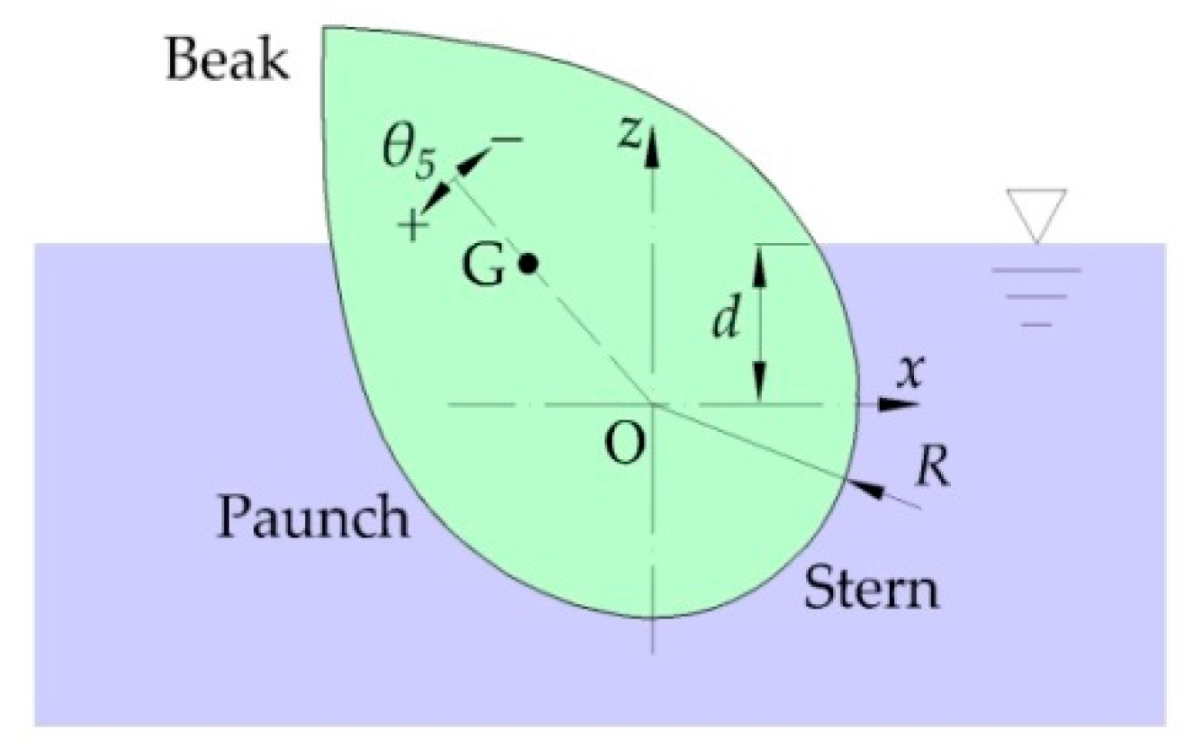
The geometry of the cross section of the solo Duck is shown in Figure 2. The cross section is composed of the paunch, stern and beak parts, and rotates about the axis O. The stern part is of circular shape with O as its center point, so that the pitch motion does not radiate waves afterward, R denotes the radius of the stern part, G denotes the mass center, θ5 denotes the pitch angular displacement of the mass center with the counterclockwise direction as positive, and d denotes the depth of the rotation axis. Oxyz is the Cartesian coordinate system with x in the incident wave propagating direction, y in the longitudinal direction of the Duck, z in the opposite direction of the gravity acceleration, and z-x plane locating at the middle cross section of the Duck along the longitudinal direction.
2.2. The Geometry of the Numerical Wave Tank
Since the solo Duck is symmetrical relative to the z-x plane, only half of the Duck is modeled to reduce the computational cost. The geometry of the numerical wave tank is shown in Figure 3. The length of the NWT is 4λ, where λ is wavelength of the incident wave, and is chosen as a result of the balance between results’ stability and computational cost. The width and water depth of the NWT is the same as the experimental setup, and is 2.5 m and 4.5 m, respectively. Since the Duck WEC is of water surface piercing type, the hydrodynamic simulation of the Duck WEC is a two-phase flow problem. Therefore, another 1 m depth above the z = 0 plane is reserved for the air phase. The wave is generated at the inlet boundary, and absorbed in the wave absorbing zone, which lasts one wavelength as [28] suggests to avoid wave reflection. The Duck is placed 1.5λ away from the inlet boundary.
2.3. Boundary Conditions
To solve the RANS equation, boundary conditions should be specified to obtain the particular solution. Boundary conditions for all physical boundaries are listed in Table 1. Waves are generated at the Inlet boundary by using the velocity inlet boundary condition appended with a user defined functionspecifying the velocity and wave height time history as in [22]. At the Outlet and Top boundaries, pressure outlet boundary condition is chosen and the open channel flow option is activated to allow for specifying pressure distribution along the z direction. At the Side, Bottom and Duck boundaries, wall boundary condition is utilized as in the experimental situation. Symmetric boundary condition is applied at the Symmetric boundary to set the velocity component inthe y direction to zero. In the wave absorbing zone, the kinetic energy of the fluid is dissipated by adding negative momentum source Sx and Sy into the momentum equations. The momentum sources are defined as:
where f is the dissipation rate, xe and xp are the position where the wave absorbing zone starts and ends, respectively, u and v are the fluid velocity in the x and y direction, respectively.
It should be mentioned that the sidewall may affect the captured power of the Duck WEC. For an axisymmetric floating oscillating water column device in a wave channel, Gomes et al. found that the sidewall will increase the captured power up to a maximum of 15% for regular waves due to the transverse sloshing mode [30]. However, for different types of WECs, the influence of the sidewall is expected to be different, since the radiated and diffracted waves, which generate transverse waves, behave differently. To quantitatively identify the influence of the sidewall in the case of the Duck WEC, captured power of the WEC should be calculated as a function of the width of the wave tank at different wave periods and wave heights, so that a database can be built for different situations of the wave tank. To keep the topic of this paper focused, the influence of the sidewall on the captured power will not be studied in detail in this paper, but is arranged as the work of the next phase.
2.4. The Mesh
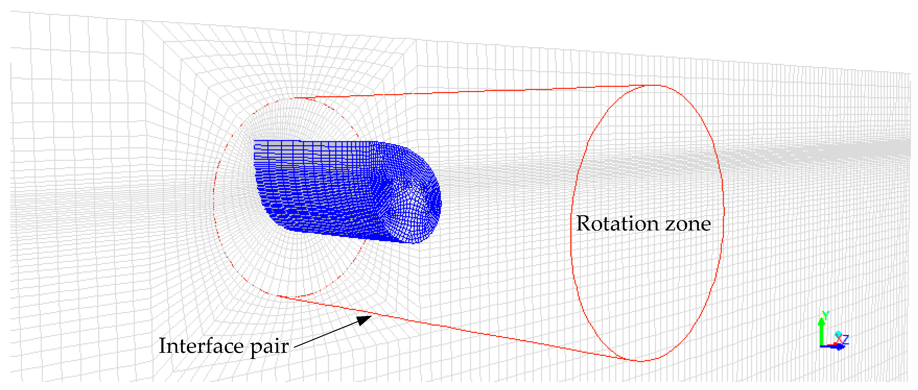
The mesh near the Duck is shown in Figure 4. Hexahedral cells are used to discretize all fluid regions. Mesh resolution is increased near both the free water surface and the end of the Duck because of relative large variability of flow parameters in these regions. A sliding mesh method is employed to model the wave interaction with the Duck by specifying the angular velocity of the rotation zone, which is kept static relative to the Duck. The data exchange between the static zone and the rotation zone is realized by a pair of overlapping circular cylinder interfaces, at where the flow variables are synchronized by interpolation. Compared to the dynamic mesh method, a sliding mesh method can avoid large element skew after large motion of the nodes so that the mesh quality can be guaranteed. The angular velocity of the rotation zone is the same as the Duck, hence can be determined from the solution of equation of motion of the Duck as:
where J is the moment of inertia of the Duck, c is the linear damping coefficient of power take-off (PTO) system, Tg and Tw are the torques applied by the gravity and hydrodynamic force of the Duck relative to O, respectively.
2.5. Solution Method
The RANS equation for the flow region is discretized by the finite-volume method (FVM). The volume of fluid (VOF) method is used to track the free surface position in this two phase (water and air) flow problem. In [23], 5 different built-in turbulence models of the ANSYS Fluent are cross compared to see their differences in modeling wave interaction with a flap-type WEC, and resultsshow that the difference can be neglected. In this paper, the renormalization group (RNG) k - ε modelis applied as the turbulence model. Boundary layer effects around walls are modeled by a standard wall function. Pressure implicit with splitting of operator (PISO) method is chosen to treat pressure-velocity coupling and pressure-based segregated solver only (PRESTO!) scheme is selected for pressure interpolation. The equation of motion of the Duck, i.e., Equation (3), is solved by the Euler method. Small time step should be chosen to not only satisfy small Courant number to increase computational stability, but also reduce local and global error of this integration method.
3. Experimental Model
The experiments were performed in the wind tunnel and water flume (HTWF) laboratory at Harbin Institute of Technology. The wave tank is 50 m long, 5 m wide and 4.5 m water depth. Both regular and irregular waves can be generated. The wave period is between 0.5 s and 5 s, and the wave height ranges from 2 cm to 40 cm. The wave height at the position of the Duck position was calibrated before the experiments. The dimension of the Duck cross section is 1:33 scaled compared to the full scale designed in [15].
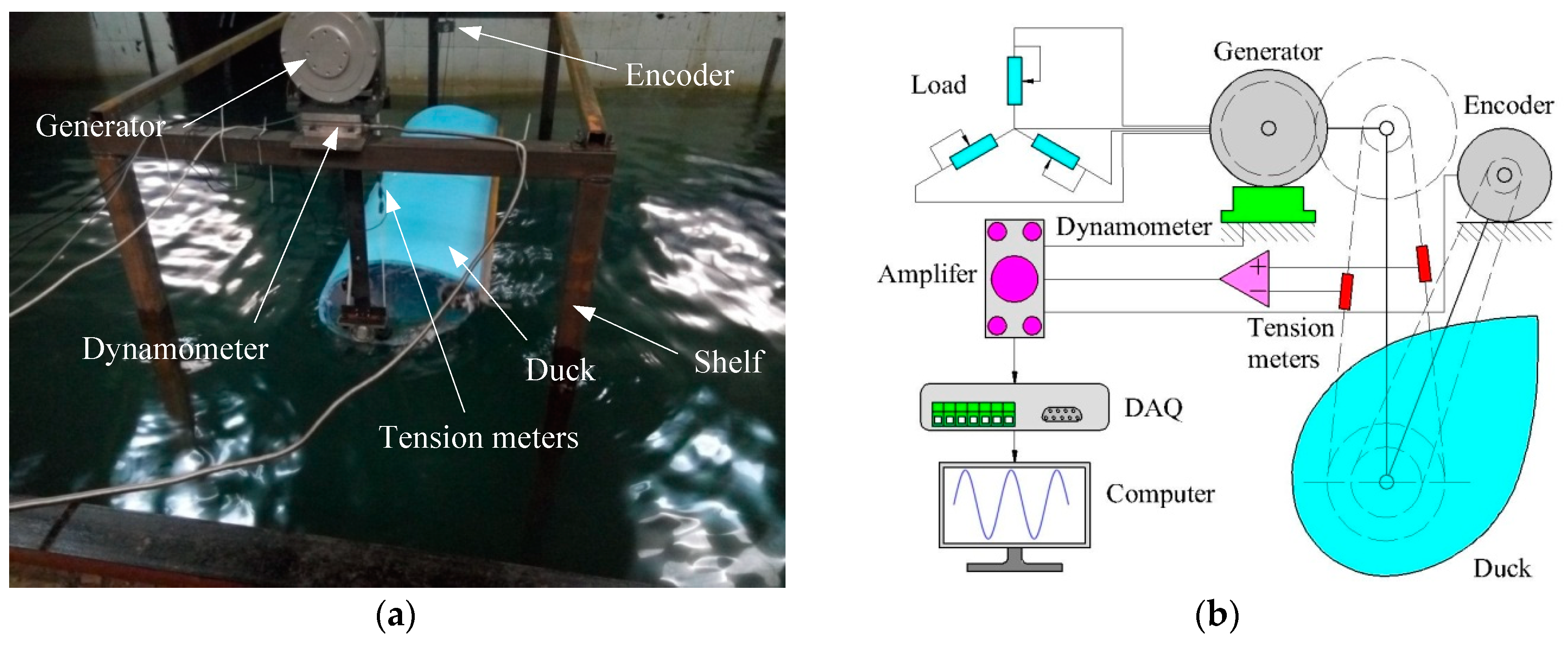
The configuration of the experimental setup is shown in Figure 5a,b. A low speed disk-type permanent magnet generator, which is often used in small wind turbines, is used as the PTO system, and it is connected to the rotation axis of the Duck by cascaded synchronizing wheels and gears to increase speed. The speed-up system will drive the generator out of the non-linear speed zone, where the output voltage is not proportional to the input rotation speed, so that the linear damping assumption in numerical simulations will be more credible. The load of the PTO system consists of symmetric three phase resistors, and the resistors are adjustable to find optimal damping coefficient for power absorption. The torque transferred by the synchronizing belt is measured by a pair of tension meters, which are embedded into the synchronizing belt on both sides. The torque can be determined by the output voltage difference between the two meters firstly multiplied by a factor, which is obtained by the multiplication of the amplification coefficient of the mechanical and electrical systems, and secondly multiplied by the radius of the synchronizing wheel. The synchronizing belt and tension meters are pre-tensioned to avoid force impact if the belt is suddenly tensioned from the slacked state. The pitch angular displacement of the Duck is measured by an encoder connected to the rotation axis of the Duck on the other side also by a synchronizing belt. A Kistler 9257B three components dynamometer is used to measure the hydrodynamic forces in surge and heave directions. It is fixed on one side of the rotation axis supporting system assuming that the hydrodynamic forces are distributed symmetrically relative to the middle section of the Duck. Output voltage signals of the all these transducers are imported to a data acquisition (DAQ) card, which transfers analog signals to digital signals, and then the output of DAQ card is transferred to a computer, where data is stored and analyzed.
In the experiment, the radius of the stern part is 0.2 m; the depth of the rotation axis is 0.05 m; and the coordinate of the mass center is (−0.038 m, 0.046 m); and the mass of the Duck is 139.2 kg. In numerical simulations, half of the Duck mass are specified since only half Duck is modeled.
4. BEM Model
For a more thorough comparison in this paper, BEM simulations are also performed to compare with both CFD and experimental results. WAMIT v7.0 [31] (Version 7.0, WAMIT Inc, Chestnut Hill, MA, USA) is employed to calculate the hydrodynamic response of the Duck in regular wave conditions. The pitch angular displacement amplitude and hydrodynamic force amplitude can be calculated from non-dimensional response amplitude operator (RAO) data by:
where θ5 and
are the dimensional and non-dimensional pitch angular displacement amplitude respectively, X1,3 and are the dimensional and non-dimensional surge and heave hydrodynamic force amplitude in the x and z direction respectively, ρ is the water density, g is the gravity acceleration, H is the wave height, and L is the characteristic length [31].
5. Results and Discussion
In this section, the convergence of the CFD model is first investigated. Then, the CFD model is validated by comparing the predicted hydrodynamic responses with both experimental and BEM results. Finally, the hydrodynamic nonlinearity identified by the CFD model and the hydrodynamic force distribution along the longitudinal direction of the Duck are studied.
5.1. Convergence Study of the CFD Model
Before the CFD model is used to perform hydrodynamic simulations of the solo Duck WEC, it should be both mesh and time step resolution independent. Figure 6a,b show the measured free surface elevation h at the Duck position with the Duck be removed from the NWT, and hydrodynamic responses of the Duck at wave period T = 1.6 s and wave height H = 0.075 m. Here, τ is the non-dimensional flow time defined by the flow time t divided by the wave period. In both subfigures, the curves behave in an approximately sinusoidal way. The variation of the measured wave height only depends on horizontal and vertical, i.e., the x and z direction, mesh resolution. Therefore, convergence of the mesh resolution in horizontal and vertical directions is investigated with measured wave height as the dependent variable. On this basis, when the Duck is embedded into the NWT, the variation of the pitch angular displacement amplitude θ5 only depends on the longitudinal, i.e., the y direction, mesh resolution and the time step resolution. Hence convergence of the longitudinal mesh resolution and the time step resolution will be studied with pitch angular displacement amplitude as the dependent variable. Since small vibrations of both H and θ5 are observed due to wave reflection, the two dependent variables are averaged over three wave periods for comparison. In Figure 6b, the surge and heave hydrodynamic forces represent the forces applied by the water in the x and z direction, respectively.
Figure 7 shows the convergence study results at T = 1.6 s and H = 0.075 m. Figure 7a shows the measured wave height as a function of the cell number per wavelength and per wave height. The wave height tends to be stable when the cell number per wavelength and per wave height exceeds 30 and 10, respectively. Figure 7b shows the pitch angular displacement amplitude as a function of the cell number in the longitudinal direction and per wave period. Also, it reveals that when the cell number in the longitudinal direction and per wave period exceeds 32 and 360, respectively, the angular displacement amplitude tends to converge. Therefore, for a tradeoff betweenthe computational costand the accuracy, for later simulations in this paper, the mesh resolution and time step are set according to the critical cell number stated above.
5.2. Comparison in Different Wave Heights
Table 2 shows the test cases for the comparison in different wave heights. Figure 8 shows the comparison of the pitch angular displacement amplitude as a function of wave height among CFD, BEM and experimental results at T = 1.6 s. In Table 2, the difference of the wave height between the CFD and experimental model is due to the measured wave height at the position of the Duck being different from the set value at the wave maker. For example, if the set value of the wave height at the wave maker is 1.0 cm, the measured value of the wave height at the position of the Duck may be smaller than 1.0 cm. The reason behind this phenomenon is that the wave energy is dissipated during the propagation process. Since the dissipation rate of the wave energy may be different between the CFD and experimental model, the measured wave height at the position of the Duck may also be different, e.g., 0.9 cm for the CFD model and 0.8 cm for the experimental model. Therefore, the expectation of realizing an identical value of the wave height at the position of the Duck for both the CFD and experimental models cannot be easily achieved, but needs time-consuming tuning of the set value of the wave height at the wave maker for both models. Besides, since the wave height is served as the independent variable in Figure 8, whether or not the wave height in the CFD and experimental model is the same does not influence the variation tendency of the dependent variable. Therefore, the wave height between the CFD and experimental model needs not to be the same. The maximum of the wave height in the CFD model is larger than that of the experimental model due to capsizing of the Duck. Due to friction, the motion response of the Duck in the experimental model is slightly smaller than that in the CFD model. Therefore, the Duck in the experimental model is harder to capsize. Meanwhile, the maximum wave height in both models is the minimum wave height that induces the Duck to capsize. Therefore, the maximum of the wave height in the experimental model is larger than the CFD model.
For all three models, the pitch angular displacement amplitude grows with wave height. CFD results agree well with BEM results at small wave heights, and presents almost linear relationship with wave height. However, at large wave heightswhen H ≥ 0.12 m, difference emerges since the CFD curve shows a slower growing trend while the BEM one shows the same slope as at small wave heights. Actually, this can be explained by the hydrodynamic nonlinearityinduced at large wave heights. In [32], it is found that BEM models without the nonlinear term of drag force over-estimate the response of the WEC when compared to CFD models. For cases with high wave heights, the influence of the drag force will be more prominent since the magnitude of the drag force increases with the square of velocity. Compared to experimental results, the CFD curve shows the same tendency as the experimental one, but predicts an overall larger value, especially at small wave heights. A possible explanation for these phenomena is the friction loss in the mechanical transmission system. Actually, friction is very complex and its formation mechanism has still not been clearly revealed yet. Friction also varies nonlinearly with a lot of parameters, such as the velocity. For a Duck WEC, since the Duck oscillates periodically, the velocity of the Duck varies all the time, thus a fixed value of the friction cannot be obtained. Han et al. [33] tried to take friction into consideration by tuning the value of the friction inside the numerical model until the response of the numerical model equals that measured in the experimental model. However, for the comparison between the numerical and the experimental model in this paper, the friction cannot be determined ahead. Anyway, although there are differences between the numerical and experimental model, the difference is not significant overall, and experimental results can still quantitatively validate the numerical models to some extent.
Figure 9 shows the comparison of the hydrodynamic force amplitude as a function of wave height at T = 1.6 s. Both surge and heave forces grow almost linearly with wave height. Similar to the variation tendency of pitch angular displacement amplitude with wave height, CFD results agree well BEM results at small wave heights, while diverges from BEM results at large wave heights with the heave force as an exception. Compared to experimental results, CFD results show only small difference in the whole wave height range. The main reason is that the friction in the mechanical transmission system does not influence the pressure distribution around the Duck. Therefore, the hydrodynamic forces are not influenced by the friction.
5.3. Comparison in Different Wave Periods
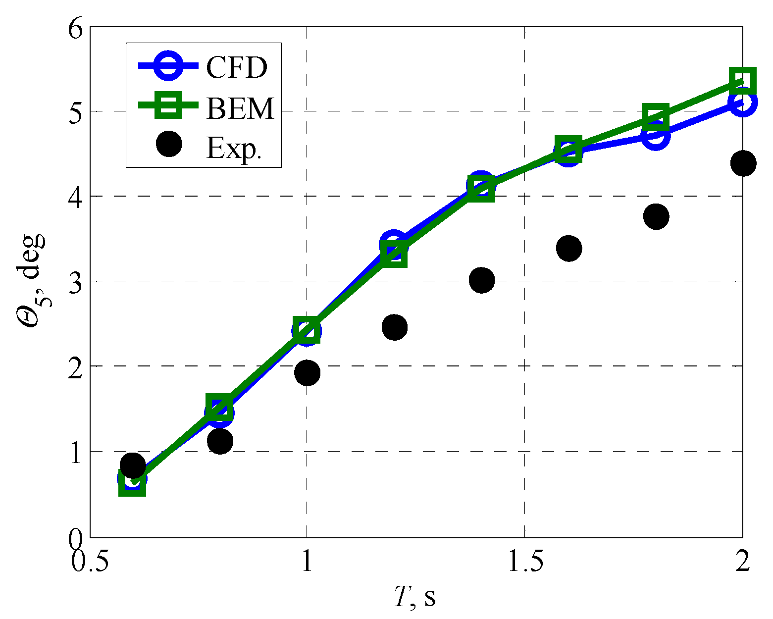
In this section, the comparison is performed in a range of wave periods, from 0.6 s to 2.0 s. Table 3 shows the test cases for the comparison in different wave periods. Figure 10 shows the comparison of pitch angular displacement amplitude as a function of wave period among CFD, BEM and experimental results at H = 0.075 m. For all three models, the angular displacement amplitude grows with wave period. CFD results agree well and almost coincides with BEM results when T ≤ 1.4 s. When T > 1.4 s, CFD results are slightly smaller than BEM results. The difference is expected to be resulted from the viscosity that damps the response of the Duck in the CFD model. The angular displacement amplitude predicted by the CFD model is larger than experimental results a most wave periods except at T = 0.6 s and the discrepancy grows with wave period.
Figure 11 shows the comparison of the hydrodynamic force amplitude as a function of wave period at H = 0.075 m. In Figure 11a, the surge force amplitude peaks at T = 1.4 s and decreases gradually on either side for all three models. The surge force amplitude of CFD resultsshow little difference from experimental resultswithin the wave period range from 0.8 s to 1.4 s, while is smaller than experimental results when T ≤ 0.8 s, and larger than them when T ≥ 1.4 s. Compared to BEM results, the force predicted by the CFD model is slightly larger in the whole wave period region. In Figure 11b, the heave force amplitude grows with wave period for all three models. In fact, these amplitudes equal the surge and heave excitation force since the WEC is static in both degrees of freedom. The shape of the curves is characterized by either a bell-like shape with the peak value appears at the wave period of 1.4 s, or by a nearly monotonically varying trend. The data that forms the shape can be approximately obtained by solving the Laplace equation, with the boundary condition defined by the geometry of the WEC. Therefore, the shape of the curves, no matter it is the bell-like form for the surge mode or the nearly straight form for the heave mode is influenced mostly by the geometry of the WEC. The difference between CFD and experimental results is smaller than that between BEM and experimental results. One possible reason for the discrepancy between CFD and experimental results may be the installation error of the mechanical equipments, which may cause the measured surge and heave excitation forces be coupled with the excitation force of other degrees of freedom. The complex coupling effect may cause the resultant measured excitation force from the experiment be larger than that of the numerical models. From above comparison results, it is revealed that the CFD model can better predict the hydrodynamic response of the Duck than the BEM model for this experimental setup.
5.4. Influence of Wave Steepness
From the comparison performed in Section 5.2 and Section 5.3, we find that the difference of the predicted hydrodynamic responses between the CFD and BEM models appears at different wave heights and wave periods.In order to quantitatively describe the difference of predicted results between the CFD and BEM model, the concept of relative difference is introduced as:
where φCFD denotes results from the CFD model and φBEM for the BEM model. Relative difference is defined to measure to what extent the two results differ from each other. Figure 12 shows the relative difference of pitch angular displacement amplitude as a function ofwave height and wave period. It can be seen that the relative difference between the CFD and BEM model generally increases with wave height, but decreases with wave period.
Since the BEM model is linearised from the CFD model, we can attribute the above difference to the hydrodynamic nonlinear factors that are taken into consideration in the CFD model, including the nonlinearity of the wave, i.e., the nonlinear waveform, and the nonlinearity of the Duck motion, i.e., the vortex generation process. High nonlinearity of the wave means relatively large wave heights, resulting in relatively large motion response of the Duck, i.e., high nonlinearity of the Duck motion. Therefore, the nonlinearity of the Duck motion is positively correlated to the nonlinearity of the wave. Therefore, the nonlinearity of the wave can be seen as an index to represent the total nonlinearity. Normally, the nonlinearity of the wave can be measured by the wave steepness defined as:
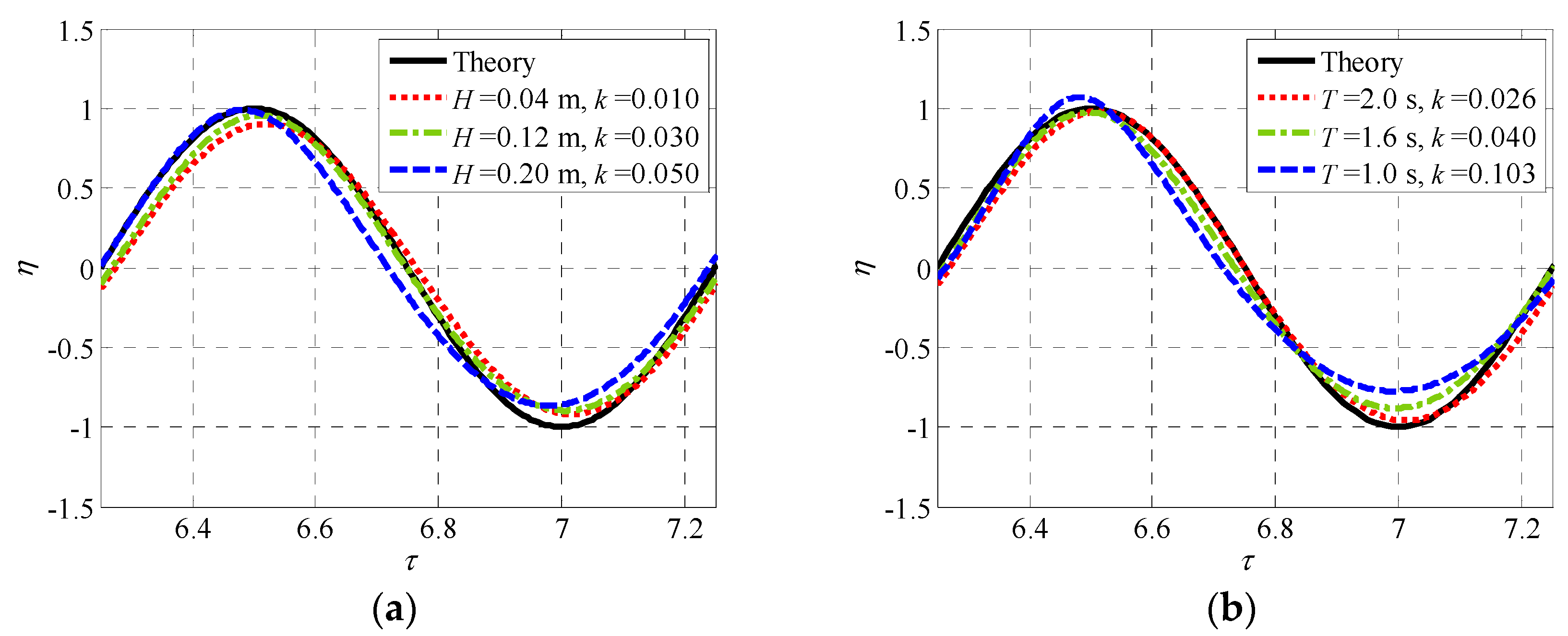
The wave steepness is also shown in Figure 12 as a set of contour lines. It can be clearly seen that the difference betweenCFD and BEM results grows with wave steepness. Figure 13 shows the non-dimensional free surface elevation, η = 2h/H, where h denotes the free surface elevation, and H denotes the wave height, as a function of the non-dimensional flow time for different wave steepness at T = 1.6 s and H = 0.16 m, respectively. When looking into Figure 13, it can be found that: with the increase of wave steepness, the wave crest becomes shaper and the wave trough becomes flatter. This process is similar to the transient process from the Airy wave to the second order Stokes wave, indicating that the nonlinearity of the wave increases with wave steepness.With the increase ofwave nonlinearity, the drift torque drives the Duck to capsize when the wave condition exceed a critical value. In this situation, since the Duck departures from its original equilibrium position, the comparison of the pitch angular displacement amplitude of the Duck between the CFD and BEM model will be meaningless. Therefore, a dashed line is shown in Figure 12 to distinguish the useful data in the left part from the useless date in the right part.
The paragraphs above attributed the difference between the CFD and BEM model to hydrodynamic nonlinear factors, and the reason can be explained as follows. The BEM model is based on the Laplace Equation, which is originated from the Navier-Stokes Equation with the assumptions of inviscid fluid, incompressible and irrotational flow. To solve the Laplace Equation, the linear wave theory, which assumes that both the wave steepness and motion response of the WEC are small, is employed. On the other hand, the CFD model used in this work is based on the RANS Equation, which is also originated from the Navier-Stokes Equation but with the turbulence effect be approximated by empirical models. Although both two models adopt approximations, the CFD model is closer to real flow conditions than the BEM model since the fluid can be viscid, and the flow can be compressible and rotational. With the increase of wave steepness, large wave steepness may violate basic assumptions of the linear wave theory, resulting in the BEM model loss the ability to accurately predict the hydrodynamic response of the WEC. Therefore, the CFD model is expected to be more accurate than the BEM model in this case.
5.5. Vortex Generation Processat the End of the Duck
In the above section, we inferred that one of the hydrodynamic nonlinear factors is from the Duck motion, which is mainly embodied by the vortex generation phenomenon around the Duck, especially at the end the Duck. In this section, we try to study the vortex generation process around the WEC using the validated CFD model. For the solo Duck WEC, the vortex generation process is a new challenge since it does not appear for the spine-connected Duck since there are almost no gaps between the Ducks. The pressure difference between the blocked flow in the front area of the Duck and free flow at the end causes vortexes to be generated, which is also very common in aerodynamic design of airplane wings [34] and wind turbine blades [35], where blade tip losses are caused by pressure differences. The flow passing the end of a Duck is similar to a steady flow passing an obstacle with leading and trailing rectangular corners, as shown in Figure 14. In the upstream, the blockage of the obstacle causes a vertical velocity component of the flow in the front area of the obstacle. At the leading corner, the sharply deceleration of the vertical velocity in the vertical wall boundary layer causes an advert pressure gradient leading to flow separation. Under the compression of the main stream, the separation zone is restricted to a limited zone, and reattachment of the boundary layer happens when the horizontal wall is suitably long. At the trailing corner, the same phenomenon appears since the horizontal boundary layer reaches another corner, and this will cause another flow separation. In both the upstream and downstream positions, standing vortexes are generated and denoted as P and Q, respectively. Because a rectangular angle is the infinite approximation of a sufficiently large curvature, the leading and trailing corners act as the fixed flow separation points for the geometry. These vortex generation phenomena are extensively studied in [36,37,38,39]. The direction of P and Q is perpendicular to plane of the main flow with the polarity be determined so that the peripheral velocity of the vortex follows the main flow.
Figure 15 shows the fluid velocity and vorticity distribution around the end of the Duck at T = 1.6 s and H = 0.12 m. In the left column, the subfigures show the approximately undisturbed fluid velocity vector distribution in the plane y = 2.4 m. The hollow circle represents the rotation axis of the pitch motion. Within a wave period, as shown in the linear wave theory, the velocity direction of water particles at a fixed point is of circular type, as shown in Figure 15i and the time sequence follows the clockwise principle as A→B→C→D→A. In the right column, vorticitydistributionof the main vortexes are shown in either the free surface, i.e., z = 0 plane, or the perpendicular surface, i.e., x= 0 plane. Since the peripheral velocity of the Duck is small relative to the fluid velocity, the Duck can be considered as standing still in the flow field. At time instance A, the main flow is in the x-y plane, i.e., z = 0 plane. As illustrated in Figure 14, the main vortexes will be generated in the z direction. The P type vortex is generated at the leading cornerat the end, while the Q type vortex is at the trailing corner, and the direction of these vortexes are both positive so that the peripheral velocity of the vortices follows the main flow, and this is confirmed in Figure 15b.
At time instance B, the main flow is in the y-z plane, i.e., x = 0. Similar to the above principle, the P and Q vortexes are generated and both in the positive x direction as confirmed in Figure 15d. At time instance C, the situation is rightly opposite to time instance A. The location of P and Q vortexes are reversed, and both are in the negative z direction as shown in Figure 15f. At time instance D, both location and direction of P and Q vortexes are reversed from time instance B as confirmed in Figure 15h.
From above discussions, we find that: at different time instances within a wave period, the magnitude and direction of the generated vortexes are different, and vary periodically. Vortexes are generated due to the relative motion between the WEC and the fluid, thus part of the kinetic energy of the WEC will be devoted to feed the vortex generation process, resulting in the captured power of the WEC be reduced.
The vortex generation process causes the static pressure in the downstream side of the obstacle be smaller than that of the upstream side, resulting in a force resisting the relative motion of the obstacle, e.g., a resisting torque for the Duck in this paper. This resisting force is called the drag force, whose magnitude is proportional to the square of the velocity and direction is opposite to the velocity. Therefore, the nonlinearity of the Duck motion, which is embodied by the vortex generation phenomenon, can be quantitatively represented by the drag torque. Besides, since the analysis in Section 5.4 revealed that the nonlinearity of the wave is positively correlated to the nonlinearity of the Duck motion, we combine the two nonlinear factors together so that the total nonlinearity is quantitatively represented by a single drag torque. As in [40], the drag torque of the Duck in the pitch degree-of-freedom can be defined as:
where Cd is the drag torque coefficient. Then, according to the Newton’s Second Law, we can obtain the equation of motion of the Duck as:
where Te is the excitation torque, Tr is the radiation torque, and Th is the hydrostatic torque. By solving Equation (9), we can obtain the motion response of the Duck in the time domain considering the drag torque. However, the drag torque coefficient in Equation (8) for a given wave condition cannot be obtained directly. In this paper, this drag torque coefficient is obtained in an indirect way as in [33], by tuning its value until the motion response of the Duck obtained from Equation (9) equals that of the CFD model.
Figure 16 shows the drag torque coefficient as a function of wave height at T = 1.6 s and c = 12 N·m·s/rad. At small wave heights, the drag torque coefficient is almost zero. However, at large wave heights, the drag torque coefficient increases significantly with wave height. This is due to the nonlinear behavior of the wave and the vortex generation phenomenon is more prominent at large wave heights. The observed variation tendency in Figure 16 indicates that the drag torque coefficient effectively reflected the influence of the nonlinearity of the wave and the Duck motion. This gives the opportunity to build a database of the drag torque coefficient as a function of wave height, wave period, etc, so that the hydrodynamic nonlinearity can be modeled with reasonable accuracy without the time-consuming CFD model.
5.6. Hydrodynamic Force Distribution Along the Longitudinal Direction of the Duck
In order for the solo Duck WEC to survive in harsh offshore climates, the hydrodynamic force distribution along the longitudinal direction of the Duck should be carefully considered in designing the intensity and stiffness of the WEC structure. Figure 17 shows the comparison of surge and heave forces per unit square meter along the longitudinal direction of the Duck among 3D CFD, pseudo 3D CFD and BEM results at t = 8.544 s when T = 1.6 s and H = 0.08 m.
The pseudo 3D CFD simulation is intended for simulating the hydrodynamic performance of the spine-connected Duck, and is implemented by applying the symmetric boundary at both ends of the Duck. Correspondingly, 3D CFD and BEM simulations are performed for the solo Duck. The hydrodynamic forces keep almost constant in the longitudinal direction in pseudo 3D CFD simulations, while vary continuously in 3D CFD and the BEM simulations, as a result of the diffracted and radiated wave in the y direction, which cannot be developed in pseudo 3D CFD simulations. This indicates that the structure design of the solo Duck should be different from that of the spine-connected Duck when considering the longitudinal force distribution. In both 3D CFD and BEM simulations, when approaching the end of Duck, the surge force decreases, while the heave force gradually increases. One interesting finding in both subfigures is the rapid jump of the forces at the end of the Duck in 3D CFD simulations, and is quite remarkable for the heave force. Figure 18 shows the comparison of the dynamic pressure contour between 3D CFD and pseudo 3D CFD simulations at t = 8.544 s, when T = 1.6 s and H = 0.075 m. It can be seen that the position where dynamic pressure dramatically varies, which is not observed in pseudo 3D CFD simulations, coincides with where vortexes are generated. Actually, the vortex generation process is due to pressure differences around the end of the Duck. The pressure near the end of the Duck quickly drops down since the vortexes take away the kinetic energy from the fluid, resulting in the rapid jump of the pressure force. The comparison shows that the CFD model can subtly capture the local feature of the vortex generation process and its influence on the hydrodynamic forces. Therefore, the CFD model is recommended for this kind of calculation. From the above discussion, it is found that the hydrodynamic forces of the solo Duck are different from that of its spine-connected counterpart. The resultant surge force of the solo Duck is smaller than the spine-connected Duck, which means that the modulus of the Duck cross section in the x direction can be reduced, and furthermore, the mooring force in this direction can also be reduced. Meanwhile, the resultant heave force of the solo Duck is also smaller, which means that the modulus of the Duck section in the z direction can be reduced, and likewise for the mooring force. Overall, the smaller dynamic surge and heave forces will reduce the fatigue load on the Duck WEC hull and the mooring system, which will result in the fatigue life of the Duck to be extended.
6. Conclusions
This paper developed a CFD model to predict the hydrodynamic performance of a solo Duck WEC in regular waves within a wide range of wave steepness until the Duck capsizes. The CFD model, in which the sliding mesh technology is employed, is validated by comparing the predicted hydrodynamic responses, i.e., the pitch angular displacement amplitude, the surge and heave hydrodynamic forces, with that predicted by the experimental and BEM models and some nonlinear phenomena are studied.
CFD results agree well with experimental results with the main difference coming from the friction brought by the mechanical transmission system. CFD results also agree well with BEM results with the difference resulting from hydrodynamic nonlinearity, which is identified as two factors that is taken into consideration in the CFD model: the nonlinearity of the wave, i.e., the nonlinear waveform, and the nonlinearity of the Duck motion, i.e., the vortex generation process. The influence of both two nonlinear factors is combined to be quantitatively represented by the drag torque. This provides the opportunity to build a database of the drag torque coefficient as a function of wave height, wave period, etc., so that these nonlinear factors can be modeled with reasonable accuracy without the time-consuming CFD model. The vortex generation phenomenon is found to cause a rapid jump of the pressure force due to the vortexes taking away the kinetic energy from the fluid. The hydrodynamic surge and heave forces and required mooring forces of the solo Duck is smaller than that of its spine-connected counterpart owing to the three-dimensional characteristic of the structure.
Author Contributions
J.W. performed the numerical simulation and prepared the manuscript. Y.Y., D.S., Z.N. and M.G. supervised the wave power project.
Funding
The research was supported by Shenzhen Science and Technology Innovation Committee Grant 20160221 and the Swedish Research Council (VR) Grant 2015-04657.
Conflicts of Interest
The authors declare no conflict of interest.
References
- Gunn, K.; Stock-Williams, C. Quantifying the global wave power resource. Renew. Energy 2012, 44, 296–304. [Google Scholar] [CrossRef]
- International Energy Agency (IEA). Key World Energy Statistics 2016; IEA: Paris, France, 2016; pp. 35–36. [Google Scholar]
- Falnes, J. A review of wave energy extraction. Mar. Struct. 2007, 20, 185–201. [Google Scholar] [CrossRef]
- Hong, Y.; Waters, R.; Bostrom, C.; Eriksson, M.; Engstrom, J.; Leijon, M. Review on electrical control strategies for wave energy converting systems. Renew. Sust. Energy Rev. 2014, 31, 329–342. [Google Scholar] [CrossRef] [Green Version]
- Salter, S.H. Wave power. Nature 1974, 249, 720–724. [Google Scholar] [CrossRef]
- Salter, S.H. Characteristics of a rocking wave power device. Nature 1975, 254, 504–506. [Google Scholar]
- Cruz, J. Ocean Wave Energy Current Status and Future Perspectives; Springer: Berlin, Germany, 2008. [Google Scholar]
- Jeffrey, D.C.; Richmond, D.J.E.; Salter, S.H.; Taylor, J.R.M. Study of Mechanisms for Extracting Power from Sea Waves; Second Year Report on Edinburgh Wave Power Project; University of Edinburgh: Edinburgh, UK, September 1976. [Google Scholar]
- Salter, S.H. The development of the Duck concept. In Proceedings of the Wave Energy Conference, London, UK, 22–23 November 1978. [Google Scholar]
- Jeffrey, D.C.; Keller, G.J.; Mollison, D.; Richmond, D.J.E.; Salter, S.H.; Taylor, J.R.M.; Young, I.A. Fourth Year Report on Edinburgh Wave Power Project; University of Edinburgh: Edinburgh, UK, 1978. [Google Scholar]
- Evans, D.V. A theory for wave-power absorption by oscillating bodies. J. Fluid Mech. 1976, 77, 1–25. [Google Scholar] [CrossRef]
- Mynett, A.E.; Serman, D.D.; Mei, C.C. Characteristics of Salter’s cam for extracting energy from ocean waves. Appl. Ocean Res. 1979, 1, 13–20. [Google Scholar] [CrossRef]
- Nebel, P. Maximising the efficiency of wave energy plant using complex-conjugate control. J. Syst. Control Eng. 1992, 206, 225–306. [Google Scholar]
- Wu, J.; Yao, Y.; Li, W.; Zhou, L.; Göteman, M. Optimizing the Performance of Solo Duck Wave Energy Converter in Tide. Energies 2017, 10, 289. [Google Scholar] [Green Version]
- Pizer, D. Numerical Modeling of Wave Energy Absorbers; Technical Report; University of Edinburgh: Edinburgh, UK, 1994. [Google Scholar]
- Cruz, J.; Salter, S.H. Numerical and experimental modeling of a modified version of the Edinburgh Duck wave energy device. Proc. Inst. Mech. Eng. Part M J. Eng. Marit. Environ. 2006, 220, 129–147. [Google Scholar]
- Cruz, J.; Salter, S. Update on the design of an offshore wave powered desalination device. In Proceedings of the OWEMES 2006-Civitavecchia, Rome, Italy, 20–22 April 2006. [Google Scholar]
- Lucas, J.; Salter, S.H.; Cruz, J.; Taylor, J.R.M.; Bryden, I. Performance optimization of a modified Duck through optimal mass distribution. In Proceedings of the 8th European Wave and Tidal Energy Conference, Uppsala, Sweden, 7–10 September 2009. [Google Scholar]
- Pastor, J.; Liu, Y. Power Absorption Modeling and Optimization of a Point Absorbing Wave Energy Converter Using Numerical Method. J. Energy Res. Technol. 2014, 136, 021207. [Google Scholar] [CrossRef]
- Pastor, J.; Liu, Y. Frequency and time domain modeling and power output for a heaving point absorber wave energy converter. Int. J. Energy Environ Eng. 2014, 5, 101. [Google Scholar] [CrossRef]
- Li, Y.; Lin, M. Regular and irregular wave impacts on floating body. Ocean Eng. 2012, 42, 93–101. [Google Scholar] [CrossRef] [Green Version]
- Hadzic, I.; Hennig, J.; Peric, M.; Xing-Kaeding, Y. Computation of flow-induced motion of floating bodies. Appl. Math. Model. 2005, 29, 1196–1210. [Google Scholar] [CrossRef]
- Wei, Y.; Rafiee, A.; Henry, A.; Dias, F. Wave interaction with an oscillating wave surge converter, Part I: Viscous effects. Ocean Eng. 2015, 104, 185–203. [Google Scholar] [CrossRef]
- Wei, Y.; Abadie, T.; Henry, A.; Dias, F. Wave interaction with an oscillating wave surge converter, Part II: Slamming. Ocean Eng. 2016, 113, 319–334. [Google Scholar] [CrossRef]
- Agamloh, E.B.; Wallace, A.K.; Jouanne, A.V. Application of fluid-structure interaction simulation of an ocean wave energy extraction device. Renew. Energy 2008, 33, 748–757. [Google Scholar] [CrossRef]
- Lopez, I.; Pereiras, B.; Castro, F.; Iglesias, G. Optimisation of turbine-induced damping for an OWC wave energy converter using a RANS-VOF numerical model. Appl. Energy 2014, 127, 105–114. [Google Scholar] [CrossRef]
- Penalba, M.; Giorgi, G.; Ringwood, J.V. Mathematical modelling of wave energy converters: A review of nonlinear approaches. Renew. Sustain. Energy Rev. 2017, 78, 1188–1207. [Google Scholar] [CrossRef]
- Windt, C.; Davidson, J.; Ringwood, J.V. High-fidelity numerical modelling of ocean wave energy systems: A review of computational fluid dynamics-based numerical wave tanks. Renew. Sustain. Energy Rev. 2018, 93, 610–630. [Google Scholar] [CrossRef]
- ANSYS Inc. ANSYS Fluent 16.2 Manual; ANSYS Inc.: Canonsburg, PA, USA, 2016. [Google Scholar]
- Gomes, R.P.F.; Henriques, J.C.C.; Gato, L.M.C.; Falcão, A.F.O. Wave power extraction of a heaving floating oscillating water column in a wave channel. Renew. Energy 2016, 99, 1262–1275. [Google Scholar] [CrossRef]
- WAMIT Inc. WAMIT User Manual Version 7; WAMIT Inc.: Chestnut Hill, MA, USA, 2013. [Google Scholar]
- Bhinder, M.A.; Babarit, A.; Gentaz, L.; Ferrant, P. Potential time domain model with viscous correction and CFD analysis of a generic surging floating wave energy converter. Int. J. Mar. Energy 2015, 10, 70–96. [Google Scholar] [CrossRef]
- Han, J.; Maeda, T.; Kinoshita, T.; Kitazawa, D. Towing test and motion analysis of motion controlled ship—Based on an application of skyhook theory. In Proceedings of the 12th International Conference on the Stability of Ships and Ocean Vehicles (STAB2015), Glasgow, Scotland, 14–19 June 2015. [Google Scholar]
- Devenport, W.J.; Rife, M.C.; Liapis, S.; Folin, G.J. The structure and development of a wing-tip vortex. J. Fluid Mech. 1995, 312, 67–106. [Google Scholar] [CrossRef]
- Wood, D.H.; Okulov, V.L.; Bhattacharjee, D. Direct calculation of wind turbine tip loss. Renew. Energy 2016, 95, 269–276. [Google Scholar] [CrossRef] [Green Version]
- Yu, D.; Kareem, A. Parametric study of flow around rectangular prisms using LES. J. Wind Eng. Ind. Aerodyn. 1998, 77–78, 653–662. [Google Scholar] [CrossRef]
- Arslan, T.; Malavasi, S.; Pettersen, B.; Andersson, H.I. Turbulent flow around a semi-submerged rectangular cylinder. J. Offshore Mech. Arct. Eng. 2013, 135, 1–11. [Google Scholar] [CrossRef]
- Sherry, M.J.; Jacono, D.L.; Sheridan, J.; Mathis, R.; Marusic, I. Flow separation characterization of a forward facing step immersed in a turbulent boundary layer. In Proceedings of the Sixth International Symposium on Turbulence and Shear Flow Phenomena, Seoul, Korea, 22–24 June 2009; pp. 1325–1330. [Google Scholar]
- Shimada, K.; Ishihara, T. Application of a modified k-ε model to the prediction of aerodynamic characteristics of rectangular cross-section cylinders. J. Fluid Struct. 2002, 16, 465–485. [Google Scholar] [CrossRef]
- Sjökvist, L.; Wu, J.; Ransley, E.; Engström, J.; Eriksson, M.; Göteman, M. Numerical models for the motion and forces of point-absorbing wave energy converters in extreme waves. Ocean Eng. 2017, 145, 1–14. [Google Scholar] [CrossRef]
Figure 1.
Configuration of Ducks: (a) spine-connected Ducks; (b) solo Ducks.

Figure 2.
Geometry of the cross section of the solo Duck.

Figure 3.
Geometry of the numerical wave tank.

Figure 4.
The mesh near the Duck.

Figure 5.
Configuration of the experimental setup: (a) physical model; (b) simplified schematic diagram.
Figure 5.
Configuration of the experimental setup: (a) physical model; (b) simplified schematic diagram.

Figure 6.
Measured free surface elevation at the Duck position with the Duck be removed from the NWT and hydrodynamic responses of the Duck at T = 1.6 s and H = 0.075 m: (a) measured free surface elevation and pitch angular displacement of the Duck; (b) surge and heave hydrodynamic forces applied on the Duck.

Figure 7.
Convergence study results at T = 1.6 s, and H = 0.075 m: (a) measured wave height as a function of the cell number per wavelength and per wave height; (b) pitch angular displacement amplitude as a function of the cell number in the longitudinal direction and per wave period.
Figure 7.
Convergence study results at T = 1.6 s, and H = 0.075 m: (a) measured wave height as a function of the cell number per wavelength and per wave height; (b) pitch angular displacement amplitude as a function of the cell number in the longitudinal direction and per wave period.

Figure 8.
Comparison of pitch angular displacement amplitude as a function of wave height among CFD, BEM and experimental results at T = 1.6 s.
Figure 8.
Comparison of pitch angular displacement amplitude as a function of wave height among CFD, BEM and experimental results at T = 1.6 s.

Figure 9.
Comparison of the hydrodynamic force amplitude as a function of wave height at T = 1.6 s: (a) surge force; (b) heave force.
Figure 9.
Comparison of the hydrodynamic force amplitude as a function of wave height at T = 1.6 s: (a) surge force; (b) heave force.

Figure 10.
Comparison of pitch angular displacement amplitude as a function of wave period between CFD, BEM and experimental results at H = 0.075 m.
Figure 10.
Comparison of pitch angular displacement amplitude as a function of wave period between CFD, BEM and experimental results at H = 0.075 m.

Figure 11.
Comparison of the hydrodynamic force amplitude as a function of wave period at H = 0.075 m: (a) surge force; (b) heave force.
Figure 11.
Comparison of the hydrodynamic force amplitude as a function of wave period at H = 0.075 m: (a) surge force; (b) heave force.

Figure 12.
Relative difference of the pitch angular displacement amplitude as a function ofwave height and wave period. Contour lines of the wave steepness are shown by solid lines, while the critical capsizing condition for the Duck is shown by the dashed line.
Figure 12.
Relative difference of the pitch angular displacement amplitude as a function ofwave height and wave period. Contour lines of the wave steepness are shown by solid lines, while the critical capsizing condition for the Duck is shown by the dashed line.

Figure 13.
Non-dimensional free surface elevation as a function of the non-dimensional flow time at different wave steepness: (a) at T = 1.6 s; (b) at H = 0.16 m.
Figure 13.
Non-dimensional free surface elevation as a function of the non-dimensional flow time at different wave steepness: (a) at T = 1.6 s; (b) at H = 0.16 m.

Figure 14.
A steady flow passing an obstacle with leading and trailing rectangular corners, and standing vortexes, P and Q, are generated as a result of the boundary layer separation.
Figure 14.
A steady flow passing an obstacle with leading and trailing rectangular corners, and standing vortexes, P and Q, are generated as a result of the boundary layer separation.

Figure 15.
Fluid velocity and vorticity distribution at the end of the Duck at T = 1.6 s and H = 0.12 m. The subfigures in the left column show the approximately undisturbed fluid velocity vector distribution in the plane y = 2.4 m, with subfigures (a,c,e,g) for time instances A, B, C and D, respectively. The subfigures in the right column show the vorticity of the main vortex in either the free surface, i.e., z = 0 plane, or the perpendicular surface, i.e., x = 0 plane, with subfigures (b,d,f,h) for time instances A, B, C and D, respectively. Subfigure (i) shows the velocity direction of water particles at different time instances.

Figure 16.
The drag torque coefficient as a function of wave height at T = 1.6 s and c = 12 N·m·s/rad.
Figure 16.
The drag torque coefficient as a function of wave height at T = 1.6 s and c = 12 N·m·s/rad.

Figure 17.
Comparison of hydrodynamic forces per square meter along longitudinal direction of the Duck among 3D CFD, pseudo 3D CFD and BEM results at t = 8.544 s when T = 1.6 s and H = 0.075 m: (a) surge force; (b) heave force.
Figure 17.
Comparison of hydrodynamic forces per square meter along longitudinal direction of the Duck among 3D CFD, pseudo 3D CFD and BEM results at t = 8.544 s when T = 1.6 s and H = 0.075 m: (a) surge force; (b) heave force.

Figure 18.
Comparison of dynamic pressure contour between 3D CFD and pseudo 3D CFD simulations at t = 8.544 s, when T = 1.6 s and H = 0.075 m: (a) 3D CFD; (b) pseudo 3D CFD.
Figure 18.
Comparison of dynamic pressure contour between 3D CFD and pseudo 3D CFD simulations at t = 8.544 s, when T = 1.6 s and H = 0.075 m: (a) 3D CFD; (b) pseudo 3D CFD.


Table 1.
Boundary conditions for all physical boundaries.
| Physical Boundary Name | Inlet | Top, Outlet | Symmetry | Duck, Side, Bottom |
|---|---|---|---|---|
| Boundary condition | Velocity inlet | Pressure outlet | Symmetry | Wall |
Table 2.
Test cases for the comparison in different wave heights.
| Tested Cases | 1 | 2 | 3 | 4 | 5 | 6 | 7 | 8 | 9 | 10 | |
| Wave height, cm | CFD model | 1.79 | 3.70 | 5.61 | 7.51 | 9.41 | 11.30 | 13.20 | 15.10 | 17.00 | 18.91 |
| Experimental model | 4.49 | 7.02 | 9.50 | 12.02 | 14.50 | 17.03 | 19.48 | 21.97 | – | – | |
| Wave period, s | 1.6 | ||||||||||
Table 3.
Test cases for the comparison in different wave periods.
| Tested Cases | 1 | 2 | 3 | 4 | 5 | 6 | 7 | 8 |
| Wave Period, s | 0.6 | 0.8 | 1.0 | 1.2 | 1.4 | 1.6 | 1.8 | 2.0 |
| Wave height, cm | 7.5 | |||||||
© 2019 by the authors. Licensee MDPI, Basel, Switzerland. This article is an open access article distributed under the terms and conditions of the Creative Commons Attribution (CC BY) license (http://creativecommons.org/licenses/by/4.0/).
Share and Cite
MDPI and ACS Style
Wu, J.; Yao, Y.; Sun, D.; Ni, Z.; Göteman, M. Numerical and Experimental Study of the Solo Duck Wave Energy Converter. Energies 2019, 12, 1941. https://doi.org/10.3390/en12101941
AMA Style
Wu J, Yao Y, Sun D, Ni Z, Göteman M. Numerical and Experimental Study of the Solo Duck Wave Energy Converter. Energies. 2019; 12(10):1941. https://doi.org/10.3390/en12101941
Chicago/Turabian StyleWu, Jinming, Yingxue Yao, Dongke Sun, Zhonghua Ni, and Malin Göteman. 2019. "Numerical and Experimental Study of the Solo Duck Wave Energy Converter" Energies 12, no. 10: 1941. https://doi.org/10.3390/en12101941
Note that from the first issue of 2016, this journal uses article numbers instead of page numbers. See further details here.