Reduction of Power Production Costs in a Wind Power Plant–Flywheel Energy Storage System Arrangement

Abstract

The paper presents issues of optimisation of a wind power plant–energy storage system (WPP-ESS) arrangement operating in a specific geographical location. An algorithm was developed to minimise the unit discounted cost of electricity generation in a system containing a wind power plant and flywheel energy storage. In order to carry out the task, population heuristics of the genetic algorithm were used with modifications introduced by the author (taking into account the coefficient of variation of the generation in the quasi-static term of the penalty and the selection method). The set of inequality restrictions related to the technical parameters of turbines and energy storage and the parameters of energy storage management has been taken into account with the application of the Powell–Skolnick penalty function (Michalewicz modification). The results of sample optimisation calculations for two wind power plants of 2 MW were presented. The effects achieved in the process of optimisation were described—especially the influence of the parameters of the energy storage management system on the unit cost of electricity generation. The use of a system with higher unit costs of energy generation compared to independently operating wind turbines was justified in the context of improving the conditions of compatibility with the power system—the strategy belongs to a power firming group.

1. Introduction

A serious problem of the power systems in many countries is the inclusion of a significant number of small (when compared to conventional power plants), dispersed sources of energy of an intermittent nature [1,2,3,4,5]. These include mainly wind power plants (both individual turbines and wind farms).

Issues which require solutions in this area are: reduction of the effects of fluctuations in active power supplied to the power system, random disconnections of wind sources of different duration, and maintenance of the quality of electricity as set out in the normative recommendations. The elimination or at least reduction of the effects of these phenomena requires the use of energy storage systems and the use of suitably designed systems and algorithms to control them.

In the case of wind energy sources, the use of energy storage systems can eliminate their short-term disconnections from the grid, as well as partially stabilise the active power supplied to the power system [6]. Despite higher investment and operating costs, compared to independently operating wind turbines, the wind power plant–energy storage system (WPP-ESS) arrangements are particularly interesting due to the extent of practical use of renewable energy sources and the growing demands regarding the quality of their operation [7].

Among the types of energy storage systems used, the most important are electrochemical, compressed air, pumped-storage plants and, increasingly, flywheel [8,9,10,11]. The choice of the type of energy storage system results from its operation type (number of charges and discharges, charging speed, service life, maximum depth of discharge, operating temperature range, etc.). In the conducted study, the authors determined that flywheel storage systems may form an alternative to electrochemical storage systems in power supply systems with renewable energy sources [12,13]. Their advantages over other types of storage systems are, in the case of wind energy: a wide range of operating temperatures (from −30 °C to 45 °C) feasible without changing the capacity, lifespan (comparable to that of the turbines), charging speed (comparable to the discharge time) and the ability to recharge from any level of charge without losing the nominal capacity. The main disadvantages of the system are high investment costs and considerations of work safety—the rotating mass rotates at speeds up to tens of thousands of revolutions per minute. Due to the presented advantages, the reminder of the paper will consider the optimisation of a system structure of the wind power plant and flywheel energy storage system (WPP-FESS) [6,8,14].

With a large variety of types of wind turbines currently in production, a highly efficient selection of a specific model for operation in a specific geographical location should be carried out using methods much more accurate than those recommended in IEC 61400-1. This statement becomes even more important in the case of a complex system, i.e., the combination of a wind turbine and a flywheel energy storage system [6,8,14]. Therefore, the authors propose that, due to the high costs of this type of design and its technical complexity, this task should be carried out with the use of an optimisation algorithm. Its aim is to search for a system structure which, in a given geographical location (known wind speed measurement data), allows for the generation of electricity at the lowest unit price.

The issues of cooperation between flywheel energy storage and wind turbines are discussed in many scientific papers. They concern different applications and aspects, e.g., technical, economic, etc. [12]. In the article [15], the authors sought, for the optimal number of wind turbines and the size of the cooperating FESS located in a specific location, to supply a known group of individual customers. Such issues coincide with the interests of the authors of the paper, as exemplified by the paper [14]. The construction and selection of parameters of regulators and energy storage system management systems is a frequent issue in the scope of cooperation between WPP-FESS [16,17,18,19,20]. Their main objective is to reduce the adverse characteristics of wind energy, especially stochastic and dynamic changes in wind speed. An interesting construction of a flywheel energy storage system cooperating with wind turbines in microgrids proposed in the paper [13], where energy is also stored in the cooperating battery, which allows to control the voltage. In the paper [17] it is shown that a flywheel energy storage with a properly designed control system can effectively compensate for fast power fluctuations caused by torque disturbances in wind turbines due to deviations in the air flow through the tower as well as by rapid fluctuations in wind power. The integration of the FESS with the DFIG system mitigates voltage fluctuations at the output of the system and allows for better use of available wind energy [19]. In another paper [20] the authors focused on the energy storage consisting of many flywheels (matrix) and developing an algorithm for controlling each flywheel in an individual way, thus limiting the power fluctuation at the output and improving the stability of energy production in a wind power plant. The use of FESS directly in the wind turbine system [21] is intended to stabilise the output power of the wind turbine and additionally to mitigate mechanical vibrations in various points of the wind turbine, which are a serious problem of mechanical structures. The incorporation of flywheel energy storages into the grid is also analysed in more complex hybrid generational systems, e.g., wind and solar, as well as with diesel generators [22]. This leads to an improvement in the quality of electricity generation, in particular frequency stabilisation.

In the analysed literature, the issues of influence of parameters of the energy storage management algorithm on unit costs of electricity generation in an optimised system WPP-FESS have not been considered so far. Therefore, in this paper the indicated topics have been taken up, with emphasis on the analysis of the impact of three parameters of the author’s algorithm of energy storage management, which is a variation of the power firming strategy, whose main objective is to shape the production profiles of energy sources. The paper attempts to determine the impact:

• the maximum duration of periods with reduced wind energy compensated by energy from the flywheel energy storage (T_MAX),
• reference power at the output of the system wind power plant–flywheel energy storage (P_3MIN),
• the interruption rate of permissible k_L determining the probability of interruption (specified by T_MAX parameter) of periods with system output power below the reference power of P_3MIN on the unit price of the energy produced, assuming that the system has an optimal structure in this respect.

As a result of the conducted analyses, the ranges of changes in the unit discounted cost of electricity generated in the system with changes in the above-mentioned parameters of energy storage management for a specific type of turbine and location of power plants were indicated. On the basis of the determined curves it is possible to assess the validity of the use of energy storages with a specific energy capacity for the indicated technical solutions of the WPP-FESS.

2. Compatibility of the Wind Power Plant–Flywheel Energy Storage System (WPP-FESS) Arrangement with the Power System

The stochastic course of changes in wind speed v_w = f(t) and the overlapping deterministic components (daily, annual and multi-annual fluctuations) lead to complex and unstable operating conditions for a wind power plant. Wind speed varies significantly, reaching values below turbine cut-in speed (v_cut-in), as well as above cut-out speed, leading to interruptions in power generation. Slightly exceeding the v_cut-in speed results in a turbine active power output of just a few percent of its rated power. Furthermore, in many geographical locations, the probability that the v_wn wind speed guaranteeing the generation of the rated power is maintained for longer periods of time is low. The characteristics of wind power and the properties of wind turbines mean that wind power plants are treated as intermittent sources of energy, which can introduce hazards to the power system, e.g., deterioration of the rates of reliability of power supply to the system [14,23,24,25,26,27]. A partial solution to this problem is the use of modern wind energy prediction systems and temporary replacement of wind turbines with other sources, e.g., conventional power plants. However, predictive systems are unable to predict short-term periods of wind energy reduction and are therefore of limited use.

Improvement of the stability of the power system with a high share of wind sources, in the case of short-term drops of wind energy below the adopted limit value, is possible through their pairing with energy storage systems [6,14,28,29]. For this purpose, the article proposes flywheel storage systems, whose properties and advantages in combination with wind turbines are presented in the introduction.

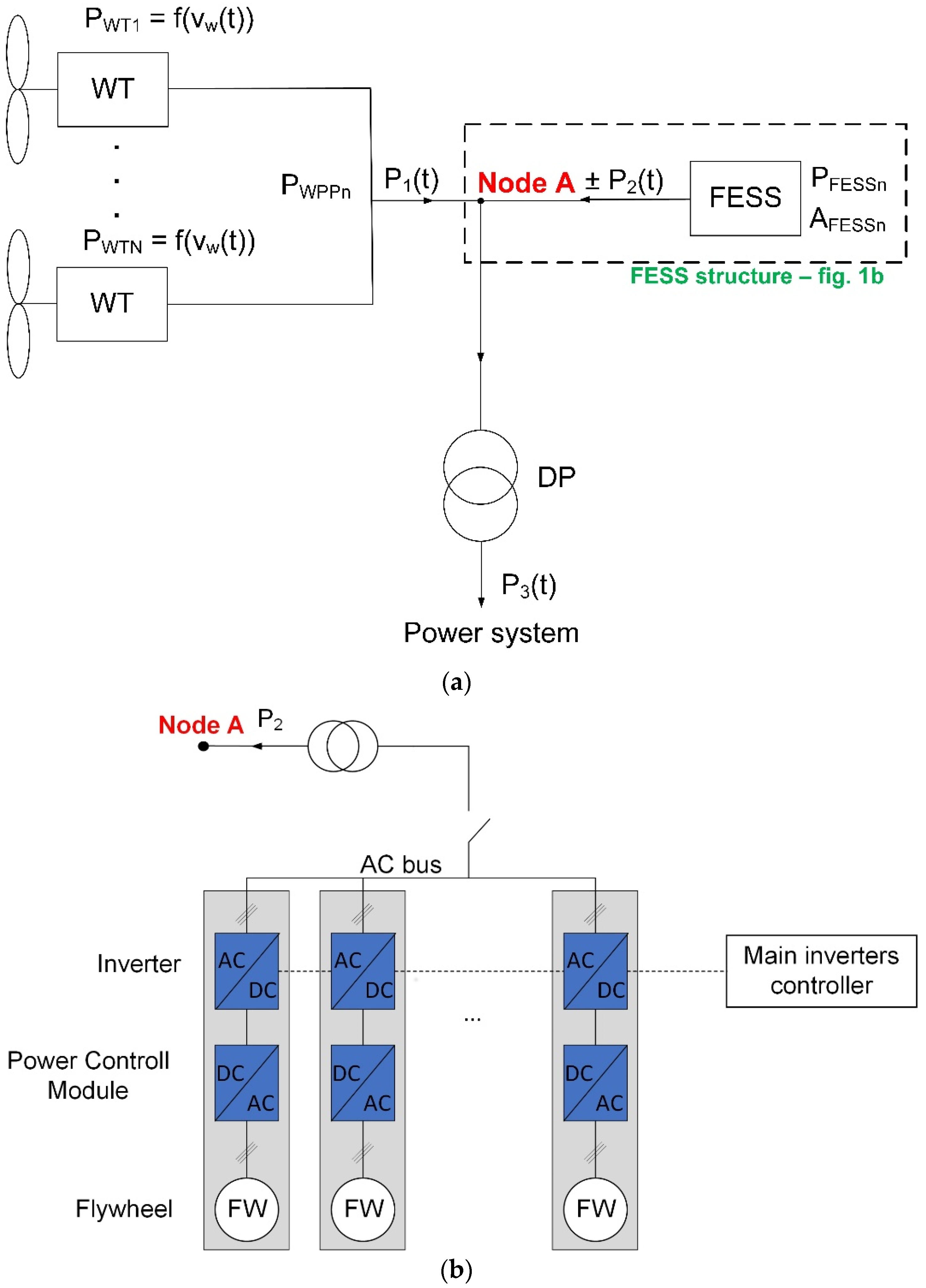
Figure 1a presents a general electrical diagram of the wind power plant–flywheel energy storage system (WPP-FESS) arrangement, where P₁ = f(t) denotes the power generated at moment t by the wind power plant, P₂ = f(t) is the power of the energy storage system (“+” indicates the discharging of the system, “–” its charging), and P₃ = f(t) is the power transferred from the system to the power grid described by the following dependence:

$${\mathrm{P}}_3\left(\mathrm{t}\right)={\mathrm{P}}_1\left(\mathrm{t}\right)\mp {\mathrm{P}}_2\left(\mathrm{t}, \mathrm{SOC}\right)-\Delta \mathrm{P}\left(\mathrm{t}\right)$$

(1)

where: SOC—state of charge of the energy storage system defined as the rate of the current amount of energy stored in the system to its nominal capacity, ΔP—power loss in systems supplying energy from the wind power plant to the power grid (the amount of losses depends on the level of power supplied to the transformer and results from the efficiency of transmission equipment, primarily the transformer).

The analysed energy storage system uses a FESS, which is an alternative to electrochemical batteries. Its selection is dictated by the adjustment of properties to the conditions of cooperation with wind turbines (large range of operating temperatures, service life comparable to that of wind turbines, the possibility of full discharge, as well as full charge and discharge performed in comparable time). The applied flywheel energy storage consists of a group of modules of equal electrical and mechanical parameters connected by a common AC bus. The module consists of: reversible electric machine with flywheel (usually made of composite material), power control module and three-phase inverter. All inverters are additionally connected to the central controller for synchronisation of the electricity parameters (Figure 1b). Examples of such structures are Power Beacon systems installed in containers or concrete underground structures.

The operation of the energy storage is managed by ESMS (energy storage management system), which in the analysed case is an original implementation of the strategy of shaping generation profiles (power firming). It consists in maintaining at output, wind power plant, power at the reference level in periods of set maximum duration (ESMS parameters). In the case of instantaneous power of wind power plant above the reference power, the energy storage is charged in order to prepare for the next periods of reduced wind energy. The task of the energy storage is therefore to minimise the periods in which the power supplied to the system from the analysed system is lower than the reference power. Details of this way of managing the flywheel energy storage are presented in articles [6,14].

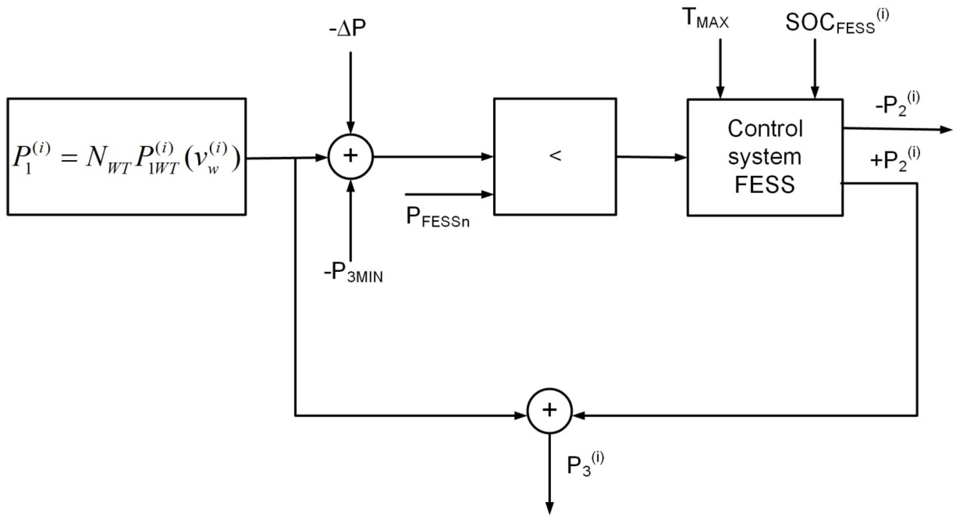
These effects are achieved by appropriately selecting the energy capacity of the storage system A_FESSn and using an algorithm to control the charging and discharging process, taking into account wind conditions, the duration of power generation interruptions and the permissible depth of discharge for the storage system. Details of the control algorithm and the results of simulation of its operation for test and real input data are presented in [6,30]. According to the assumptions adopted therein, the role of the energy storage system is to supplement the power supplied to the power grid up to the value of P_3MIN in periods of reduced power generation by the wind power plant (when P₁ − ΔP < P_3MIN) and the duration of a single cycle not longer than T_MAX. The block diagram of the joint operation of the storage system and the wind power plant described above, including the determination of the charging or discharging capacity of the flywheel storage system, is presented in Figure 2.

3. Modelling of the Operation of the Wind Power Plant–Flywheel Energy Storage System Arrangement

The analysis of the operation of the system described in point 2 requires the development of mathematical and numerical models. When developing these models, it is necessary to take into account the purpose of the analysis, which is to determine the amount of power generated in the WPP-FESS system over a period of one year. This is the basic input data to determine the structure of the system that minimises the cost of electricity production in the type of generation systems under consideration. The purpose of the simulation tests defined in such a way allows for the exclusion of dynamic states from the model (both mechanical and electrical parts), so that the mathematical model of the system may be significantly simplified [14].

Measurements of wind speed from south-eastern Poland from the years 2008–2012 made by Ph.D. Krzysztof Markowicz were used as input function in the analysis of the simulated operation of the WPP-FESS system. The wind speed averaging time is Δt = 47 s, which leads to the processing of more than 670 thousand samples for the period of one year. The measurements were taken at an altitude of 10 m above ground level and calculated according to the exponential profile of wind speed changes [14,31], to the actual height of the turbine. Using the above i-th measurement sample refers to time t⁽ⁱ⁾ = i∙Δt for i = 1, 2, …, N. Further in the article, the ^“(i)” notation will be used for marking the values of wind power and speed for the i-th measurement sample and the energy values of the storage system in the i-th Δt period.

For the purpose of simulating the WPP-FESS system and the described form of input data (input function), it is necessary to determine the partial energies generated by the wind power plant and the energy of the storage system for subsequent wind speed measurement samples.

Assuming the given simplifications, the wind turbine model is reduced to a block representing its power characteristics P_1WT = f(v_w(t)). Using linear interpolation between two points of discrete turbine power characteristics, the power generated for the i-th wind speed sample ${\mathrm{P}}_{1\mathrm{WT}}^{\left(\mathrm{i}\right)}=\mathrm{f}\left({\mathrm{v}}_{\mathrm{w}}\left({\mathrm{t}}^{\left(\mathrm{i}\right)}\right)\right)=\mathrm{f}\left({\mathrm{v}}_{\mathrm{w}}^{\left(\mathrm{i}\right)}\right)$ can be determined from the dependence:

$${\mathrm{P}}_{1\mathrm{WT}}^{\left(\mathrm{i}\right)}=\{\begin{array}{c}{\mathrm{P}}_{\mathrm{v}1+}\frac{{\mathrm{P}}_{\mathrm{v}2}-{\mathrm{P}}_{\mathrm{v}1}}{{\mathrm{v}}_2-{\mathrm{v}}_1}\left({\mathrm{v}}_{\mathrm{w}}^{\left(\mathrm{i}\right)}-{\mathrm{v}}_1\right) \mathrm{for} {\mathrm{v}}_{\mathrm{cut}-\mathrm{in}}\le {\mathrm{v}}_{\mathrm{w}}^{\left(\mathrm{i}\right)}<{\mathrm{v}}_{\mathrm{wn}}\\ \\ {\mathrm{P}}_{1\mathrm{WTn}} \mathrm{dla} {\mathrm{v}}_{\mathrm{wn}}\le {\mathrm{v}}_{\mathrm{w}}^{\left(\mathrm{i}\right)} < {\mathrm{v}}_{\mathrm{ut}-\mathrm{out}}\\ \\ 0 \mathrm{for} \mathrm{other} {\mathrm{v}}_{\mathrm{w}}^{\left(\mathrm{i}\right)}\end{array}$$

(2)

where v₁, v₂—wind speed values at discrete turbine power characteristics, between which is the speed v_w⁽ⁱ⁾ ∈ <v₁;v₂>, P_v1 and P_v2—the turbine power corresponding to wind speeds v₁ and v₂ read from discrete power characteristics, v_wn—wind speed at which the wind turbines obtain rated power, P_WPPn—rated power of the wind power plant.

The power of a power plant with N_WT turbines for the i-th sample of wind speed is determined from the dependence:

$${\mathrm{P}}_1^{\left(\mathrm{i}\right)}={\displaystyle \sum }_{\mathrm{j}=1}^{{\mathrm{N}}_{\mathrm{WT}}}{\mathrm{P}}_{1\mathrm{WT}\left(\mathrm{j}\right)}^{\left(\mathrm{i}\right)}({\mathrm{v}}_{\mathrm{w}}^{\left(\mathrm{i}\right)})$$

(3)

where j—turbine index.

According to the WPP-FESS system operation algorithm described in chapter 2, fluctuations in power input to the power grid from the wind power plant are compensated to P_3MIN with the P₂ storage system capacity when the generated power falls below P_3MIN (P₃ > P_3MIN). The level of power compensation depends on the time of reduction of the output of the wind power plant (maximum length T_MAX), maximum power of the storage system and its current state of charge SOC_FESS, which for the i-th calculation step is described by the dependence:

$${\mathrm{SOC}}_{\mathrm{FESS}}^{\left(\mathrm{i}\right)}={\mathrm{A}}_{\mathrm{FESS}}^{\left(\mathrm{i}\right)}/{\mathrm{A}}_{\mathrm{FESSn}}$$

(4)

where: A_FESS—current state of energy in the storage system, A_FESSn—rated energy capacity of the storage system.

The applied model of the flywheel storage system enables the determination of the amount of energy which remains in the storage system in the i-th calculation step. This value depends on the previous (i − 1) state of charge of the storage system and the current (i) state of the system, and can be described by the following dependencies:

• for the n-load state of the energy storage system:

  $${\forall }_{\mathrm{i}} {\mathrm{SOC}}_{\mathrm{FESS}}^{\left(\mathrm{i}\right)}>0\%\cap {\mathrm{P}}_2^{\left(\mathrm{i}\right)}=0;\hspace{1em}{\mathrm{A}}_{\mathrm{FESS}}^{\left(\mathrm{i}\right)}={\mathrm{A}}_{\mathrm{FESS}}^{(\mathrm{i}-1)}-{\mathsf{\beta }\mathrm{P}}_{\mathrm{FESSn}}\Delta \mathrm{t}$$

  (5)

  where: β—percentage standby losses of the storage system relative to the rated power P_FESSn,
• for the discharging state of the storage system:

  $${\forall }_{\mathrm{i}} {\mathrm{SOC}}_{\mathrm{FESS}}^{\left(\mathrm{i}\right)}>0\%\cap {\mathrm{P}}_2^{\left(\mathrm{i}\right)}>0; {\mathrm{A}}_{\mathrm{FESS}}^{\left(\mathrm{i}\right)}={\mathrm{A}}_{\mathrm{FESS}}^{(\mathrm{i}-1)}-{\mathsf{\beta }\mathrm{P}}_{\mathrm{FESSn}}\Delta \mathrm{t}-\frac{{\mathrm{P}}_2^{\left(\mathrm{i}\right)}\Delta \mathrm{t}}{{\mathsf{\eta }}_{\mathrm{FESS}}}$$

  (6)

  where: ${\mathrm{P}}_2^{\left(\mathrm{i}\right)}$—energy storage system capacity for the i-th sample, η_FESS—charging and discharging efficiency of the storage system,
• for the charging state of the storage system:

  $${\forall }_{\mathrm{i}} {\mathrm{SOC}}_{\mathrm{FESS}}^{\left(\mathrm{i}\right)}<100\%\cap {\mathrm{P}}_2^{\left(\mathrm{i}\right)}<0;\hspace{1em}{\mathrm{A}}_{\mathrm{FESS}}^{\left(\mathrm{i}\right)}={\mathrm{A}}_{\mathrm{FESS}}^{(\mathrm{i}-1)}-{\mathsf{\beta }\mathrm{P}}_{\mathrm{FESSn}}\Delta \mathrm{t}+{\mathsf{\eta }}_{\mathrm{FESS}}{\mathrm{P}}_2^{\left(\mathrm{i}\right)}\Delta \mathrm{t}$$

  (7)

The storage system power ${\mathrm{P}}_2^{\left(\mathrm{i}\right)}$ is a function of the power deficit Δ${\mathrm{P}}_3^{\left(\mathrm{i}\right)}$ = P_3MIN − ${\mathrm{P}}_1^{\left(\mathrm{i}\right)}$ + ΔP < 0, the nominal power rating of the storage system P_FESSn and its previous state of charge ${\mathrm{SOC}}_{\mathrm{FESS}}^{(\mathrm{i}-1)}$:

$${\mathrm{P}}_2^{\left(\mathrm{i}\right)}=\mathrm{f}({\mathrm{P}}_{\mathrm{FESSn}}, \Delta {\mathrm{P}}_3^{\left(\mathrm{i}\right)},{\mathrm{SOC}}_{\mathrm{FESS}}^{(\mathrm{i}-1)})$$

(8)

For the i-th step of the calculation this value, with Δ${\mathrm{P}}_3^{\left(\mathrm{i}\right)}$ < 0, is determined from the dependence:

$${\forall }_{\mathrm{i}} {\mathrm{SOC}}_{\mathrm{FESS}}^{\left(\mathrm{i}\right)}>0\%;\hspace{1em}{\mathrm{P}}_2^{\left(\mathrm{i}\right)}=\min ({\mathrm{P}}_{\mathrm{FESSn}}, {\mathrm{P}}_{3\mathrm{MIN}}^{}-{\mathrm{P}}_1^{\left(\mathrm{i}\right)}+\Delta \mathrm{P})$$

(9)

When the storage system is discharged to ${\mathrm{SOC}}_{\mathrm{FESS}}^{\left(\mathrm{i}\right)}$ = 0% or the T_MAX time for one-time compensation is exceeded, the storage capacity of ${\mathrm{P}}_2^{\left(\mathrm{i}\right)}$ assumes a value of 0, which may lead to supplying the grid with power lower than the reference value (${\mathrm{P}}_3^{\left(\mathrm{i}\right)}$ < P_3MIN).

4. Optimisation of Power Production Costs in the Wind Power Plant–Flywheel Energy Storage System Arrangement

4.1. Optimisation Objective, Unit Costs of Electricity Generation

One of the groups of requirements for modern technical systems is economic indices [30,31,32,33,34]. Designing a system that meets technical assumptions and limitations, and at the same time a group of economic indices, requires the use of advanced calculation methods, among which optimisation occupies a special place [14,32,33,34,35,36,37,38,39]. It allows to choose the best solution from the point of view of the adopted quality index, called in the theory of optimisation, the objective function J(x), where x is the vector of decision variables related to the examined system and influences the value of the adopted index.

For the analysed arrangement of wind power plant–flywheel energy storage system, an important issue and at the same time the main aim of the article is the reduction of the unit cost of electricity generation, while meeting all technical limitations (described in item 2 herein).

One of the methods for comparing energy facilities intended for electricity production, in the aspect mentioned above, is the UNIPEDE (International Union of Producers & Distributors of Electrical Energy) [30] method of discounted unit cost of energy production. The method is based on discounted values, both in the area of investment and operating costs as well as the amount of electricity produced. For this purpose, the discounting factor a_y = (1 + p)^−y is used, where p is the interest rate of the loan and y is the index of the year of investment or operation. Increasing the accuracy of its calculation requires taking into account inflation (the effective interest rate is then p_r) and unplanned (emergency) shutdowns of wind turbines. The second of the elements is implemented with the use of the time availability coefficient (turbine operation) dA ∈ <0;1> [30].

For the d_A parameter of constant value for all T_E years of operation of the facility and taking into account inflation, the discounted unit cost of electricity generation k_j is defined by the dependence [30]:

$${\mathrm{k}}_{\mathrm{j}}={\mathrm{k}}_{\mathrm{jI}}+{\mathrm{k}}_{\mathrm{jE}}=\frac{{{\displaystyle \sum }}_{\mathrm{y}=0}^{{\mathrm{T}}_{\mathrm{I}}-1}{\mathbf{K}}_{\mathrm{i}\left(\mathrm{y}\right)}{\mathbf{C}}_{\mathrm{i}\left(\mathrm{y}\right)}^{\mathrm{T}}{\left({1+\mathrm{p}}_{\mathrm{r}}\right)}^{-\mathrm{y}}}{{{\displaystyle \sum }}_{\mathrm{y}=1}^{{\mathrm{T}}_{\mathrm{E}}}{\mathrm{A}}_{\left(\mathrm{y}\right)}{\mathrm{d}}_{\mathrm{A}}{\left({1+\mathrm{p}}_{\mathrm{r}}\right)}^{-\mathrm{y}}}+\frac{{{\displaystyle \sum }}_{{\mathrm{y}=\mathrm{T}}_{\mathrm{I}}}^{{\mathrm{T}}_{\mathrm{I}}{+\mathrm{T}}_{\mathrm{E}}}\left({\mathbf{K}}_{\mathrm{e}\left(\mathrm{y}\right)}^{}{\mathbf{C}}_{\mathrm{e}\left(\mathrm{y}\right)}^{\mathrm{T}}+{\mathrm{A}}_{\left(\mathrm{y}\right)}{\mathrm{k}}_{\mathrm{p}\left(\mathrm{y}\right)}^{}-{\mathrm{H}}_{\left(\mathrm{y}\right)}\right){\left({1+\mathrm{p}}_{\mathrm{r}}\right)}^{-\mathrm{y}}}{{{\displaystyle \sum }}_{\mathrm{y}=1}^{{\mathrm{T}}_{\mathrm{E}}}{\mathrm{A}}_{\left(\mathrm{y}\right)}{\mathrm{d}}_{\mathrm{A}}{\left({1+\mathrm{p}}_{\mathrm{r}}\right)}^{-\mathrm{y}}}$$

(10)

where: k_jI, k_jE—investment and operating component of the discounted unit cost of electricity generation, (y)—year of investment or operation index, p_r—effective interest rate for loans, K_i(y), K_e(y)—vectors of investment and operating components incurred in year y, C_i(y), C_e(y)—constant vectors (0 or 1) taking into account the share of particular investment and operating components in year y, A_(y)—electricity produced in year y, k_p(y)—cost of fuel used to produce a unit of energy in year y, P_(y)—installed power in year y, T_P(y)—operating time with P_(y) power in year y, T_E—life of the power plant (operation lifetime), T_I—investment period, H_(y)—sales revenues from other types of energy produced in year y.

The main components of investment costs, in the case of the WPP-FESS system, are related to the purchase of turbines and energy storage facilities; however, the costs of energy resources analysis and project documentation cannot be omitted. Considering the arrangement of a wind power plant with a N_WT number of turbines with energy storage systems (number of storage systems—N_WE), the vector K = _i(y), for the investment project carried out for a period longer than one year, for year y takes the following form:

$${\mathbf{K}}_{\mathrm{i}\left(\mathrm{y}\right)}=\left[{\displaystyle \sum }_{\mathrm{k}=1}^{{\mathrm{N}}_{\mathrm{WT}}}{\mathrm{K}}_{\mathrm{TW}\left(\mathrm{y}\right)\left(\mathrm{k}\right)},{\displaystyle \sum }_{\mathrm{k}=1}^{{\mathrm{N}}_{\mathrm{WT}}}{\mathrm{K}}_{\mathrm{TTW}\left(\mathrm{y}\right)\left(\mathrm{k}\right)},{\displaystyle \sum }_{\mathrm{k}=1}^{{\mathrm{N}}_{\mathrm{WT}}}{\mathrm{K}}_{\mathrm{MTW}\left(\mathrm{y}\right)\left(\mathrm{k}\right)},{\displaystyle \sum }_{\mathrm{k}=1}^{{\mathrm{N}}_{\mathrm{WT}}}{\mathrm{K}}_{\mathrm{FTW}\left(\mathrm{y}\right)\left(\mathrm{k}\right)},{\displaystyle \sum }_{\mathrm{n}=1}^{{\mathrm{N}}_{\mathrm{ME}}}{\mathrm{K}}_{\mathrm{ME}\left(\mathrm{y}\right)\left(\mathrm{n}\right)},{\mathrm{K}}_{\mathrm{DP}\left(\mathrm{y}\right)},{\mathrm{K}}_{\mathrm{AZE}\left(\mathrm{y}\right)}\right]$$

(11)

where: k, n—wind turbine and energy storage system indices, K_TW(y)(k)—cost of purchasing the k-th wind turbine in year y, K_TTW(y)(k)—cost of transporting the k-th wind turbine to the installation site in year y, K_MTW(y)(k)—cost of installing the k-th wind turbine in year y, K_FTW(y)(k)—cost of site preparation and construction of foundations for the k-th wind turbine in year y, K_ME(y)(n)—total cost of the n-th energy storage system with control systems and transport in year y, K_DP(y)—cost of design documentation prepared in year y, K_AZE(y)—cost of analysis of energy resources in year y.

The basic components of operating costs include the maintenance and servicing of turbines, energy storage systems and other electrical equipment. The description also takes into account the costs of land lease (the investment costs associated with the purchase of land are then assumed to be zero) and labour costs of personnel operating the system. Taking into account the above elements, the operating components vector K_e(y) for year y can be expressed as:

$${\mathbf{K}}_{\mathrm{i}\left(\mathrm{y}\right)}=\left[{\displaystyle \sum }_{\mathrm{k}=1}^{{\mathrm{N}}_{\mathrm{WT}}}{\mathrm{K}}_{\mathrm{KTW}\left(\mathrm{y}\right)\left(\mathrm{k}\right)}^{},{\displaystyle \sum }_{\mathrm{n}=1}^{{\mathrm{N}}_{\mathrm{ME}}}{\mathrm{K}}_{\mathrm{KME}\left(\mathrm{y}\right)\left(\mathrm{n}\right)}^{},{\mathrm{K}}_{\mathrm{KO}\left(\mathrm{y}\right)}^{},{\mathrm{K}}_{\mathrm{D}\left(\mathrm{y}\right)}^{},{\mathrm{K}}_{\mathrm{OP}\left(\mathrm{y}\right)}^{}\right]$$

(12)

where: K_KTW(y)(k)—maintenance cost of the k-th turbine in year y, K_KME(y)(n)—maintenance cost of the n-th energy storage system in year y, K_KO(y)—maintenance cost of equipment in year, K_D(y)—land lease cost in year y, K_OP(y)—labour costs in year y.

4.2. Objective Function, Decision Variables, Restrictions

The index, defined by the relationship (10), binds the amount of energy generated, the technical structure of the system and the costs incurred during the investment and operation periods. It also takes into account the important aspect of change in the value of money over time. In many cases, it is the economic aspect that determines whether or not to implement energy investment projects. It was, therefore, considered that the objective function in the form of (10) would be used as an indicator of the quality of solution J(x) in the process of reducing the costs of electricity generation in the wind power plant–flywheel energy storage system arrangement. The investment part of the k_jI index corresponds to the investment part of the objective function J_I(x) and the k_jE operational part to the operational part of the objective function J_E(x):

$$\mathrm{J}\left(\mathbf{x}\right)={\mathrm{J}}_{\mathrm{I}}\left(\mathbf{x}\right)+{\mathrm{J}}_{\mathrm{E}}\left(\mathbf{x}\right)$$

(13)

The search for a solution to the analysed task is carried out in the area of acceptable solutions X, which is limited by a set of inequality conditions. In addition to the structural constraints imposed on decision variables, a set of functional restrictions shall also be taken into account. They are related to the control of the fit of the WPP-FESS system parameters determined by calculation with the assumed values. It is, therefore, necessary to take into account all restrictions in the objective function (13). The method of the exterior penalty function [x] has been used for this purpose, for which the modified objective function J_M(x) takes the form:

$${\mathrm{J}}_{\mathrm{M}}\left(\mathbf{x}\right)={\mathrm{J}}_{\mathrm{I}}\left(\mathbf{x}\right)+{\mathrm{J}}_{\mathrm{E}}\left(\mathbf{x}\right)+{{\displaystyle \sum }}_{\mathrm{i}=1}^{{\mathrm{N}}_{\mathrm{CON}}}{\mathrm{F}}_{\mathrm{k}\left(\mathrm{i}\right)}\left(\mathbf{x}, {\mathsf{\rho }}_{\mathrm{i}}\right)$$

(14)

where: N_CON—number of structural and functional restrictions, F_k(i)(x, $\mathsf{\rho }$_i)—penalty function for the i-th restriction, $\mathsf{\rho }$_i—scalar penalty coefficient for the i-th restriction.

The forms of penalty functions for particular restrictions are determined individually, and their correct definitions have a significant impact on the effectiveness of the optimisation process. The value of the coefficient $\mathsf{\rho }$_i affects the amount of the penalty in relation to the original value of the objective function (13) and is determined in such a way as to adequately approximate the exact solution.

Analysis of the physical structure of the WPP-FESS system, the algorithm of interface with the power grid (item 2 herein) and the adopted criterion for solution quality assessment (13) allow the determination of the structure of the decision variables vector x for the task of reducing the unit costs of electricity generation in the wind power plant–flywheel energy storage system arrangement. It was assumed that the power plant in question is built of N_WT identical wind turbines. Subsequent elements of the vector x symbolise: x₁—type of wind turbine, x₂—N_TW number of wind turbines, x₃—height of the wind turbine tower, x₄—type of energy storage system, x₅—N_ME number of energy storage modules.

The variables listed are found in the objective function in an implicit form, and their values are related to the investment component (dependency (11)) and operational component (dependency (12)).

In the task of minimising the objective function (15), inequality restrictions are taken into account, including: N_TW—number of wind power plants, N_ME—number of storage systems, P_WPPn—rated power of the power plant, A_FESSn—rated capacity of the flywheel energy storage system, P_FESSn—power of the energy storage system, and rate of elimination of permitted interruptions k_L.

The last of these parameters is related to the stochastic nature of the wind speed variations. The elimination of all periods with reduced wind power plant performance (P₃ < P_3MIN) and unit duration up to T_MAX is theoretically possible, but only for a very large storage system capacity, which generates additional investment costs. Therefore, in the algorithm of interface between the turbine and the energy storage system, it is assumed that the elimination of interruptions takes place with the assumed probability of k_L. The k_L index is, therefore, the ratio of the total duration of periods of reduced wind power plant performance (P₃ < P_3MIN) and unit duration up to T_MAX compensated by energy from the flywheel storage to the total duration of all periods of operation below P_3MIN in durations up to T_MAX (including uncompensated periods) in the assumed period of analysis.

Taking these restrictions into account allows the reduction of the size of the search area X, which results in shortening of analysis time.

Determining the minimum cost per unit of electricity produced in the electricity system—objective function form (14)—makes it possible to assess the degree to which the wind power plant–flywheel energy storage system arrangement is matched to its geographical location (wind conditions).

In the case of the WPP-FESS arrangement, revenues from sales of other types of energy H^(t) = 0 for t = 1, 2, …, T_E. Similarly, the cost of fuel equals zero (k_p = 0) which makes dependence (10) and consequently the objective function take a shorter form.

Determination of the value of the quality index (14) requires the determination of the amount of energy generated by the system in the assumed analysis period. The value of energy produced in year y by the wind power plant can be determined on the basis of the power curve of its turbines P_1WT = f(v_w) and information on wind speeds.

The total energy generated in the WPP-FESS system and introduced into the power grid in year y (A_S(y)) can be described by the dependence:

$${\mathrm{A}}_{\mathrm{S}\left(\mathrm{y}\right)}={\mathrm{A}}_{\mathrm{WPP}\left(\mathrm{y}\right)}-{\mathrm{A}}_{\mathrm{A}\left(\mathrm{y}\right)}-\Delta \mathrm{A}-{\mathrm{A}}_{\mathrm{FESS}+\left(\mathrm{y}\right)}+{\mathrm{A}}_{\mathrm{FESS}-\left(\mathrm{y}\right)}+\left({\mathrm{A}}_{\mathrm{FESSb}\left(\mathrm{y}\right)}-{\mathrm{A}}_{\mathrm{FESSe}\left(\mathrm{y}\right)}\right)$$

(15)

where: N_WT—number of wind turbines in power plants, A_WPP(y)—energy generated by the power plant in year y, A_A(y)—energy lost during emergency (random) interruptions of the turbine operation in year y, ΔA—energy losses in the systems supplying energy from the wind power plant to the power grid, A_FESS+(y)—total energy supplied from the storage system to the grid in year y (discharge), A_FESS-(y)—total energy drawn from the generator by the energy storage system in year y (charging), A_FESSb(y), A_FESSe(y)—energy stored in the storage system at the beginning and end of year y respectively.

The value of electricity A_WPP generated by the wind power plant consisting of N_WT identical wind turbines over a period of one year can be determined on the basis of the measured wind speed variations and the power curve of the turbine P_1WT(v_w). Using dependence (2), the energy generated during year y is determined from the dependence:

$${\mathrm{A}}_{\mathrm{WPP}\left(\mathrm{y}\right)}={\mathrm{N}}_{\mathrm{WT}}\Delta \mathrm{t}{{\displaystyle \sum }}_{\mathrm{i}=1}^{\mathrm{N}}{\mathrm{P}}_{1\mathrm{WT}}^{\left(\mathrm{i}\right)}\left({\mathrm{v}}_{\mathrm{w}}^{\left(\mathrm{i}\right)}\right)$$

(16)

where: N—number of wind speed measurement samples per year y.

The value of the energy lost during emergency interruptions A_A(y) can be identified by determining, on the basis of statistical analysis of the wind speed measurement curves, the average power P_1AVG(y) with which the wind turbines of the power plant in question operate during year y. In this case, the following dependence applies:

$${\mathrm{A}}_{\mathrm{A}\left(\mathrm{y}\right)}={\mathrm{N}}_{\mathrm{WT}}{\mathrm{T}}_{\mathrm{WT}\left(\mathrm{y}\right)}{\mathrm{P}}_{1\mathrm{AVG}\left(\mathrm{y}\right)}\left({1-\mathrm{d}}_{\mathrm{A}}\right)$$

(17)

where: T_WT(y)—operating time of a single wind turbine in year y, d_A—time availability coefficient d_A ∈ <0.1>.

The values of the remaining components occurring in dependence (15) related to the total energy returned from the storage system to the system in year y A_FESS+(y), energy drawn by the storage system in year y A_FESS-(y) during charging and the state of energy stored in the storage system at the beginning and end of the analysis period A_FESSb, A_MFESSe, as well as energy losses are determined on the basis of the applied algorithm of interface of the WPP-FESS system with the power grid and dependences from (1) to (9).

4.3. Selection and Characteristics of the Optimisation Method

The selection of the optimisation method for the analysed task is determined first of all by: the form and nature of the objective function and the method of including the set of restrictions (structural and functional).

On the basis of the completed analyses, it was found that objective function (14), adopted for the task of reducing the discounted cost of electricity generation, is multi-modal and the vector of decision variables x is heterogeneous. Variables x₂ and x₅ are integers, while the others take values from finite (countable) sets. In addition, decision variables in the modified objective function J_M(x) (14) are found in implicit form.

Taking into account the above and the properties of optimisation algorithms, it has been established that this task should be solved using a method belonging to the heuristics group. Among them, population methods show high effectiveness. Their main features, in addition to the capability of searching for the global extreme, are: resistance to the modification of the scope and complexity of the task, set of restrictions and form of the objective function, as well as possibility of application for differentiating the types of decision variables [34,40].

Among the population heuristics, particularly effective for the optimisation of complex technical objects, is the genetic algorithm (GA) [41,42], which combines the characteristics of stochastic methods with a determined implementation of functional blocks. A very important feature of the method is the wide array of possibilities of modification of algorithm elements (adjustment to the characteristics of the performed task and improvement of convergence, and natural features favouring the implementation of paralleling procedures (acceleration of calculations [30]).

Therefore, the authors assume that a modified genetic algorithm (GA) method will be used to reduce the unit discounted cost of electricity generation in the analysed system.

In the GA model, the block positional recording method with parameter standardisation was used to code the information on decision variables. The vector of independent variables x of a single individual shall be coded in binary form as one chromosome. Individual variables have numbers of genes adjusted to their nature and required recording precision and are located in fixed positions.

The characteristics of the genetic algorithm lead to the maximisation of the J_M(x) objective function, while the task under consideration involves the process of minimising the quality index (14). Therefore, the non-negative adaptation function described by the following dependence is used to assess the quality of solutions:

$$\mathrm{eval}\left(\mathbf{x}\right)=\mathrm{F}\left(\mathbf{x}\right)=\max \left\{{\mathbf{J}}_{\mathrm{M}}\left(\mathbf{x}\right)\right\}-{\mathrm{J}}_{\mathrm{M}}\left(\mathbf{x}\right)\ge 0$$

(18)

where: J_M(x)—set of values of the modified objective function for the individuals of the processed generation, J_M(x)—value of the modified objective function in the form (15).

An important issue, from the point of view of the effectiveness of the genetic algorithm, is how to take into account the penalty function. In practice, several solutions are applied, including the removal of inadmissible individuals from the processed generation—the so-called “death penalty” [43]. Such action, however, leads to an excessively rapid reduction in the diversity of the generation and, consequently, to convergence deterioration. Too weak a penalty for the best unacceptable individuals may result in a better adaptation value than that of the weaker acceptable individuals. This may eliminate some of the acceptable solutions or limit the number of their copies in the next generation. Therefore, for the discussed issue, the exterior penalty function was implemented using the Powell–Skolnick method of penalty correction with modifications by Michalewicz and the authors. This method allows the maintenance of the ability to control the individual composition of the generation, but does not introduce a significant increase in calculation time. It is achieved by splitting penalties into two parts: static and corrective, depending on the parameters of the processed population. The authors have introduced their own modification to the method, which consists of changing the part of the static penalty into a quasi-static penalty. It is assumed that the value of the r_PS method constant does not depend on the number of iterations and changes linearly as a function of the coefficient of variation V for the adaptation of individuals of the processed generation. The adaptation coefficient V is understood as the ratio of standard deviation σ to the average adaptation value of the processed generation [30]. The penalty, therefore, changes as a function of the relative change in the spread of adaptation around the mean value for subsequent generations. With the method defined above, the modified function of the target has the following form:

$${\mathrm{J}}_{\mathrm{M}}\left(\mathbf{x}\right)=\mathrm{J}\left(\mathbf{x}\right)+{\mathrm{r}}_{\mathrm{PS}}({\mathrm{V}}^{\left(\mathrm{k}\right)}){{\displaystyle \sum }}_{\mathrm{j}=1}^{\mathrm{m}}{\mathrm{w}}_{\mathrm{j}}{\mathrm{F}}_{\mathrm{kj}}\left(\mathbf{x}\right)+\mathsf{\lambda }\left(\mathrm{k}, \mathbf{x}\right)$$

(19)

where: r_PS(V^(k))—quasi-static method constant, V^(k)—coefficient of variation for generation k, w_j—weights for the individual components of the penalty function, λ(k, x)—corrective element related to the parameters of the generation currently being processed.

The change in the value of the r_PS constant takes place in a linear range from r_PSmin = 1 (for V ≤ 35%) to r_PSmax = 1.5 (for V ≥ 75%). This allows the final phase of the iterative process to increase the interval between the best- and worst-case values, which enables a stronger impact on the reproduction process. This original element of the genetic algorithm improves the convergence of the method, which allows the acquisition of an optimal solution in a shorter time.

The value of the λ(k, x) coefficient for the minimisation task will take the form:

$$\mathsf{\lambda }\left(\mathrm{k}, \mathbf{x}\right)=\{\begin{array}{c}0, \mathbf{x}\in \mathbf{X}\\ {\max }_{\mathbf{x}\in \mathrm{X}}\left\{\begin{array}{c}{0,\max }_{\mathbf{x}\in \mathrm{X}}\left[\mathrm{J}\left(\mathbf{x}\right)\right]-{\min }_{\mathbf{x}\notin \mathrm{X}}\left[\mathrm{J}\left(\mathbf{x}\right)\right]+\\ {+\mathrm{r}}_{\mathrm{PS}}({\mathrm{V}}^{\left(\mathrm{k}\right)}){\displaystyle {\displaystyle \sum }_{\mathrm{j}=1}^{\mathrm{m}}}{\mathrm{w}}_{\mathrm{j}}{\mathrm{F}}_{\mathrm{kj}}\left(\mathbf{x}\right)\end{array}\right\}, \mathbf{x}\notin \mathbf{X}\end{array}$$

(20)

where: ${\max }_{\mathbf{x}\in \mathrm{X}}\left[\mathrm{J}\left(\mathbf{x}\right)\right]$—adaptation value of the worst-case scenario, ${\min }_{\mathbf{x}\notin \mathrm{X}}\left[\mathrm{J}\left(\mathbf{x}\right)\right]+{\mathrm{r}}_{\mathrm{PS}}({\mathrm{V}}^{\left(\mathrm{k}\right)}){{\displaystyle \sum }}_{\mathrm{j}=1}^{\mathrm{m}}{\mathrm{w}}_{\mathrm{j}}{\mathrm{F}}_{\mathrm{kj}}\left(\mathbf{x}\right)$—the value of the adaptation function for the best unacceptable solution (including the quasi-static penalty element).

On the basis of literature analysis and own research [14,22,44], random selection according to the remainders with automatic change of probability was applied as a selection mechanism. The number of copies of an individual passed down to the next generation is determined by the proportion of the total expected value. It is defined as the ratio of the individual’s adaptation to the mean adaptation of the current generation. The fractional part r_F of this value is the probability that the individual will be drawn into the parent pool using multiple Bernoulli’s attempts. After each draw, the c_w coefficient from the interval (0,1) is be subtracted from the fractional part r_F. The value of this coefficient is determined from the family of characteristics c_w(r_F) for three typical interval values of the coefficient of variation of the adaptation function: V $\le$ 35%, 75% $>$ V $>$ 35% and V $\ge$ 75% [30].

Another important modification applied to GA is also the linear (as a function of the generation number) change in the number of the strongest individuals passed down to the next generation—element of the elite strategy. In the first iteration, one individual is passed down, then this number increases until the assumed iteration number is reached and is stabilised at the value of 2% of the population of the generation.

4.4. Computer Science Implementation of the Algorithm for Structure Optimisation of a Wind Power Plant—Flywheel Energy Storage System

Using the proposed models of components of the WPP-FESS system (dependences 2 to 9), the basis of the algorithm of its interface with the power grid (diagram in Figure 2) and the method of determining the discounted unit cost of electricity generation (dependence 10), as well as the modified genetic algorithm, a computer model and software were developed to search for the structure of the WPP-FESS system which minimises the unit cost of electricity generation, in a specific geographical location. The Visual Studio Professional 2010 environment was used to implement this system.

In addition to the WPP-FESS system structure optimisation algorithm in the developed system, an input and output interface of the application, module for operating the wind turbines and energy storage systems database, as well as numerical algorithms used in determining the value of the adjustment function and the value of penalties were also implemented. These include: statistical analysis of wind speed measurements and simulation of system operation in actual input functions. In order to increase the efficiency of the calculation system, a cache-type software structure was used, with the task to store and quickly find references to previously conducted analyses. The purpose of using such a structure is to prevent a recalculation of a previously analysed individual.

The most complex elements of the WPP-FESS system optimisation application, from the computer science perspective, are the system operation simulator and the paralleled method of genetic algorithm. The basic input data are: the measured wind speed from the geographical location under consideration for a period of one year, the nominal power of the system, the maximum permissible periods of reduced wind energy, the minimum power maintained by the system during these periods P_3MIN and the set of turbines and energy storage systems included.

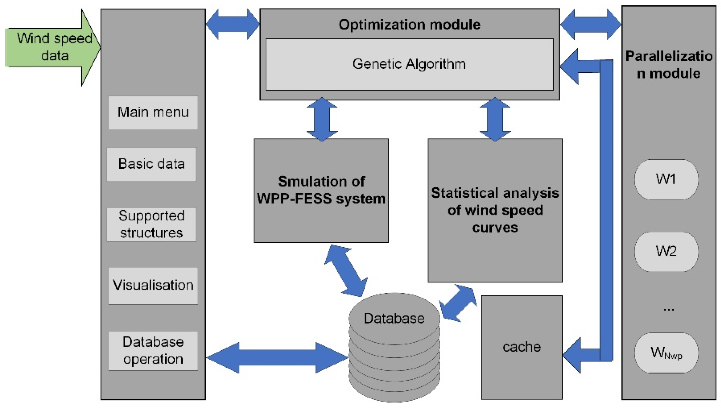
Due to time-consuming calculations, in the practical implementation of the computer system, the algorithm for paralleling the genetic algorithm with the use of master-slave architecture [30] was also applied. In connection with the intended use of the developed algorithm for implementation on PC, computer software techniques contained in the TPL library (Task Parallel Library) of the .NET platform were applied for paralleling the computational procedures. The use of the Task class and related mechanisms enables high boosts on computers equipped with multi-core processors (for the i7 950 processor, the boost for the size of tasks performed reaches 5.5). Figure 3 shows a block diagram of the application designed to optimise the wind power plant–flywheel energy storage system arrangements.

5. Results

With the use of the implemented computer system, optimisation calculations were carried out for the wind power plant–flywheel energy storage system with the rated power of P_WPPn = 2 MW. Due to the actual power output of the wind turbines stored in the database, changes in the P_WPPn rated power of the optimised system were allowed in the range of ±10%. For the adopted system and wind speed measurement data for a period of five years (2008–2012), tests were carried out in the following scopes:

• minimisation of the unit cost of electricity generation (sum of investment and operating components) in the adopted layout without energy storage systems,
• changes in the unit cost of electricity generation in an optimised WPP-FESS system in relation to optimal layouts without energy storage systems,
• minimisation of the unit cost of electricity generation in the analysed WPP-FESS system as a function of the allowable interruption index k_L for constant P_3MIN power values and time T_MAX,
• changes in the unit cost of electricity generation in the optimised WPP-FESS system as a function of P_3MIN power for fixed values of the allowable interruption elimination index k_L for time T_MAX,
• changes in the unit cost of electricity generation in an optimised WPP-FESS system as a function of T_MAX time for fixed values of the allowable interruption index k_L and power P_3MIN.

In all conducted studies, the genetic algorithm with the following parameters was applied: number of individuals N_P = 50; number of generations N_L = 100; probability of crossbreeding p_c = 0.6; probability of mutation p_m = 0.05; minimum and maximum number of individuals passed down within the dynamic elite strategy N_Smin = 1; N_Smax = 4. Parameters of the genetic algorithm have been established on the basis of preliminary tests including the determination of off-line and on-line effectiveness and the authors’ experience in issues of similar nature.

All analyses were carried out for wind measurement data between the years 2008 and 2012 from one geographical location, described in item 3 of this paper.

In the process of optimisation carried out using the method of genetic algorithm, subsequent generations contain a significant number of acceptable solutions. They represent correct technical structures (meeting the assumed restrictions) within the value of the adopted quality index of the solution worse than the final solution. For heuristic methods, the final solution can only be close to optimal, and additionally, in subsequent launches of the algorithm may change slightly. For this reason, in order to identify its quality in a given algorithm launch, the following parameter is determined:

$$\mathsf{\delta }=\frac{{\mathrm{k}}_{\mathrm{jAVG}}{\mathrm{k}}_{\mathrm{jMIN}}}{{\mathrm{k}}_{\mathrm{jAVG}}}$$

(21)

binding the unit cost k_jMIN of the best individual with the average unit cost k_jAVG of all acceptable solutions found in a full iterative genetic algorithm process.

Due to the random nature of the genetic algorithm, the δ_AVG parameter also known as the average relative decrease in unit cost (quality indicator of the solution) was defined to compare the effects of conducted analyses. This is the average value of the coefficient (21), expressed as a percentage, calculated from N_w = 20 samples:

$${\mathsf{\delta }}_{\mathrm{AVG}}=\frac{{{\displaystyle \sum }}_{\mathrm{i}=1}^{20}{\mathsf{\delta }}^{\left(\mathrm{i}\right)}}{{\mathrm{N}}_{\mathrm{W}}}·100\%$$

(22)

where: i—sample number, i = 1, 2, …, N_w.

In the case of the system type analysed in the paper, it is practically impossible to obtain detailed information on the costs of purchase, installation and maintenance of wind power plants and flywheel storage systems with the required configurations (powers and capacities). This is due to the dependence of equipment, installation and maintenance prices on the number of units, specifications and location of the facility, previous purchases and individual commercial contracts, as well as trade secrets. Therefore, the analyses used the average costs related to wind turbines converted into 1 MW of installed power and a period of one year. In the case of energy storage, the costs converted into energy unit capacity (1 kWh) and a period of one year were used. For wind power plant calculations, the data included in the report “Wind energy in Poland” [45], and for flywheel energy storage in the report “DOE/EPRI 2012 Electricity Storage. Handbook in Collaboration with NRECA” were used [46]. All adopted values have been recalculated for 2018 as the start of operation date. The methodology for developing an analytical model, numerical model and implementation of a computer optimisation system enables us to conduct research both for the data on costs, defined as described, and accurate values obtained from manufacturers.

All calculations were carried out with the use of a database containing 45 wind turbines from the following manufacturers: ENERCON, GAMESA, NORDEX and VESTAS with power outputs ranging from 0.8 MW to 4.5 MW, and three types of Power Beacon flywheel storage systems with capacities of 6, 25 and 100 kWh. Discrete power curves included in the catalogues of wind turbine manufacturers, determined for air density ρ_p = 1225 kg/m³, were used in the calculations. Wind speed at rotor hub height was calculated according to the exponential profile of wind speed changes [22].

For wind speed measurement data from 2008–2012, the structure of wind power plants without an energy storage system was optimised. It is tantamount to the optimal selection of wind turbines for the specific geographical location, taking into account the minimisation of the discounted unit cost of electricity generation by the system.

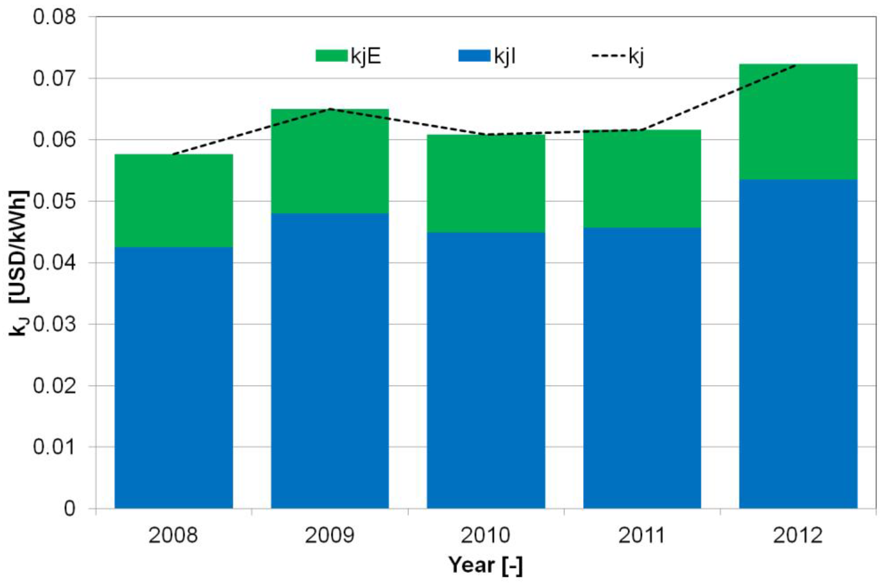
For all these years, the optimal solution is the Gamesa G 114 wind turbines with a tower height of 93 m and a unit power rating of 2 MW. This is due to the characteristics of the turbine, particularly its power characteristics adjusted to wind conditions in the analysed geographical location. The optimised values of the discounted unit cost of energy production divided into investment (k_jI) and operational (k_jE) components, without energy storage system, are presented in Figure 4.

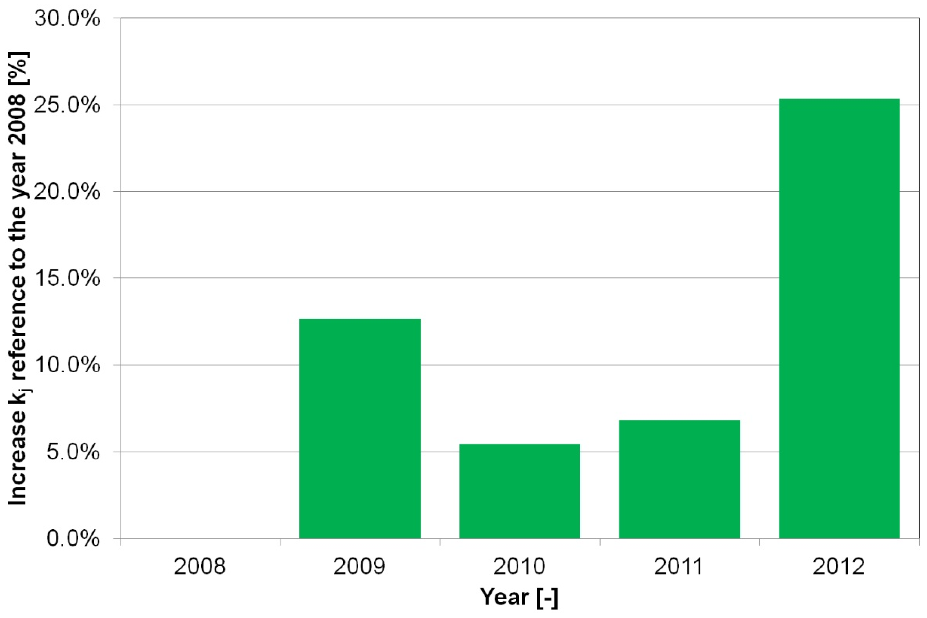
The increase in the value of the discounted unit cost of energy generation in an optimised system without energy storage for the years 2008–2012 in relation to 2008 (best wind conditions) is presented in Figure 5.

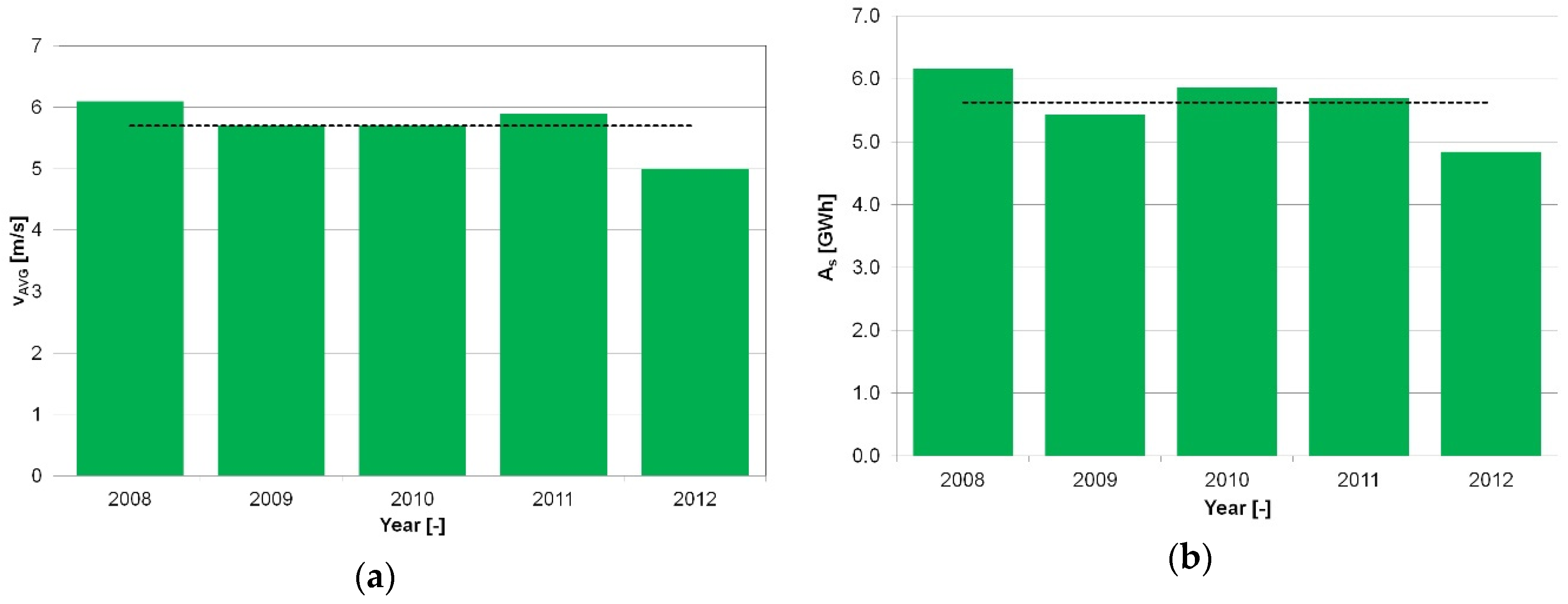
Analysing wind speeds from 2008–2012, the average annual wind speed v_Avg was determined at the height of 93 m (Figure 6a) and electric power. As supplied to the power grid over a period of one year by the optimised power plant (Figure 6b). The dashed lines indicate the average values of the aforementioned parameters in the analysed years (2008–2012).

Based on the results obtained, it was established that the best wind conditions (the highest amount of energy generated) in the period 2008–2012 occurred in 2008, wind conditions were close to the average in 2011, and the worst occurred in 2012. Therefore, further research will be carried out and compared for years: 2008, 2011 and 2012.

The optimal WPP-FESS system solutions have been determined for the selected years.

Table 1. Optimisation results for years: 2008 (best wind conditions), 2011 (average wind conditions), 2012 (worst wind conditions) and system parameters: P_3MIN = 300 kW, T_MAX = 900 s, k_L ≥ 0.7.

Parameter	Calculation Year
	2008	2011	2012
J(x) [USD/kWh]	0.147	0.169	0.196
Ji(x) [USD/kWh]	0.126	0.146	0.171
Ji(x)/J(x) [%]	85.6	86.2	87.2
Je(x) [USD/kWh]	0.021	0.023	0.025
Je(x)/J(x) [%]	14.4	13.8	12.8
Turbine type	G 114	G 114	G 114
Rated power of the turbine [kW]	2000	2000	2000
Tower height hw [m]	93	93	93
Number of turbines [pcs.]	1	1	1
Rated power of the power plant PWPPn [MW]	2	2	2
Power to grid As [GWh/a]	6.16	5.69	4.84
Rated capacity of the energy storage module [kWh]	25	25	100
Rated power of the energy storage module [kW]	100	100	250
Number of energy storage modules per turbine [pcs./turbine]	43	48	12
Capacity of energy storage system AFESSn [MWh]	1.075	1.2	1.2
Power P3MIN [kW]	300	300	300
Time TMAX [s]	900	900	900
Coefficient kL [–]	0.71	0.71	0.70
Average relative decrease in the quality of the solution δAvg [%]	25.3	24.1	26.1

presents the results of the reduction of unit costs of electricity generation for the following system input data: P_WPPn = 2 MW, k_L $\ge$ 0.7; T_MAX = 900 s; P_3MIN = 300 kW (15% P_WPPn).

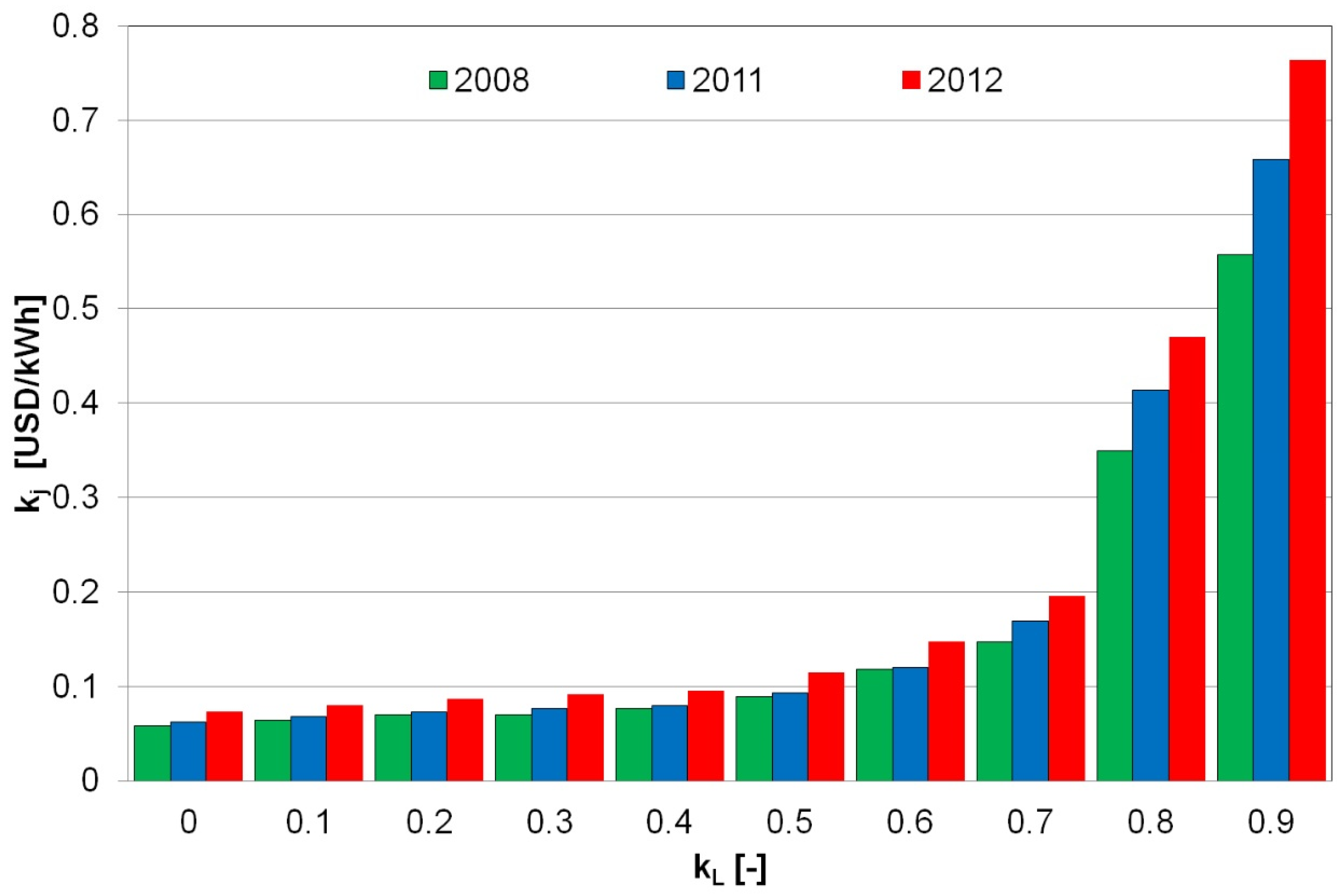
An important parameter for the operation of the analysed WPP-FESS system is the index of elimination of allowable interruptions k_L. Therefore, Figure 7 presents changes in the value of the discounted unit cost of electricity generation as a function of the allowable interruption index for the optimised system in 2008, 2011 and 2012.

Similar tests were carried out for P_3MIN power maintained at the output of the WPP-FESS system during periods of reduced wind energy. On the basis of the obtained results, it was established that the real range of variations in the k_L value was within the interval of <0;0.7>. In the case of P_3MIN power, the rapid increase in the discounted unit cost of energy generation kj occurs after exceeding 15% of the P_WPPn power. Therefore, it seems that further increases in k_L and P_3MIN warrant the use of very large energy storage capacities, whose costs are economically unjustified even in the context of improving energy quality and conditions of interface between the WPP-FESS system and the power system. Therefore, further detailed studies were carried out for the k_L index from the interval of <0;0.7> and the power P_3MIN from the interval of <0;15%P_WPPn>.

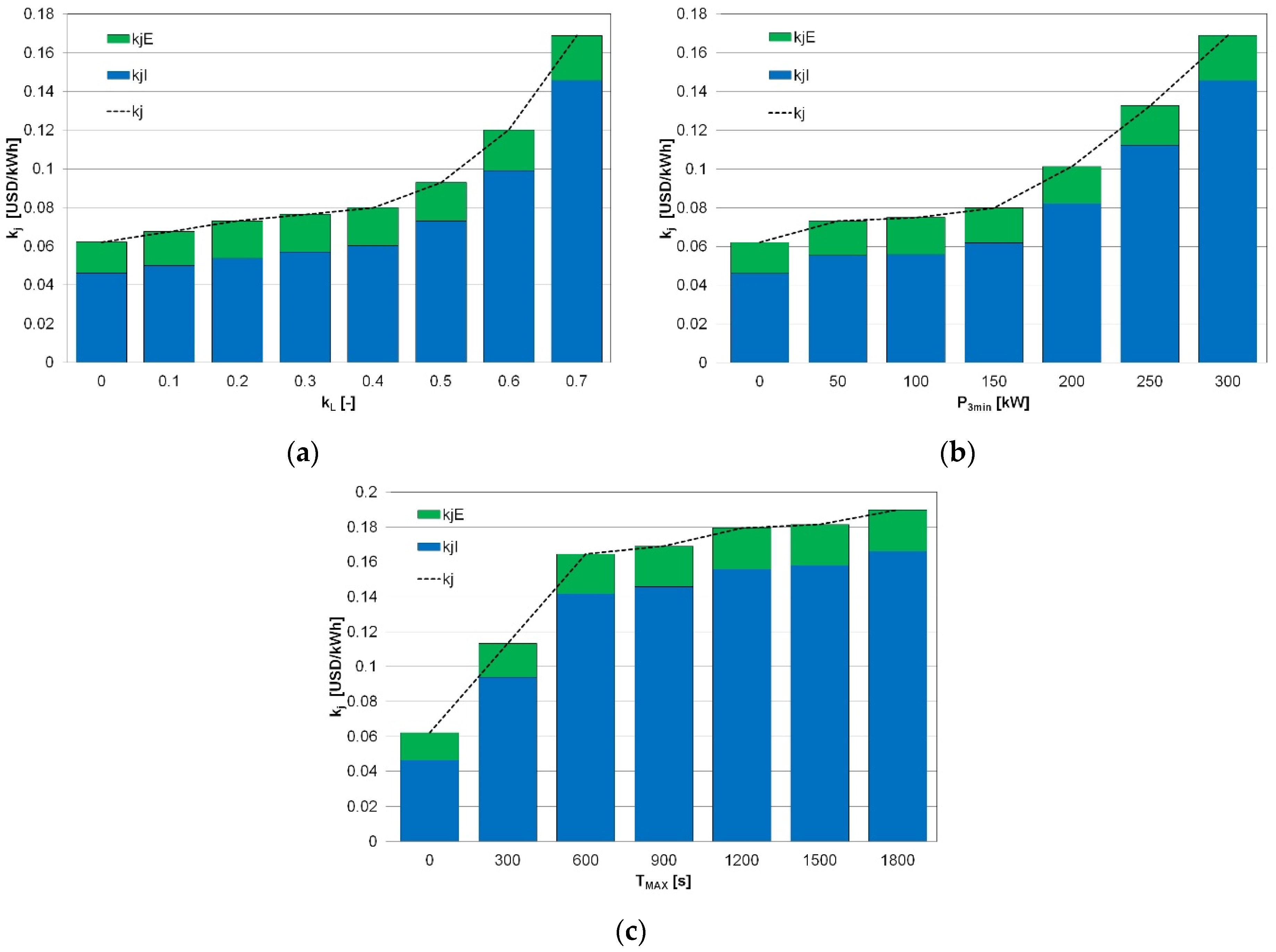
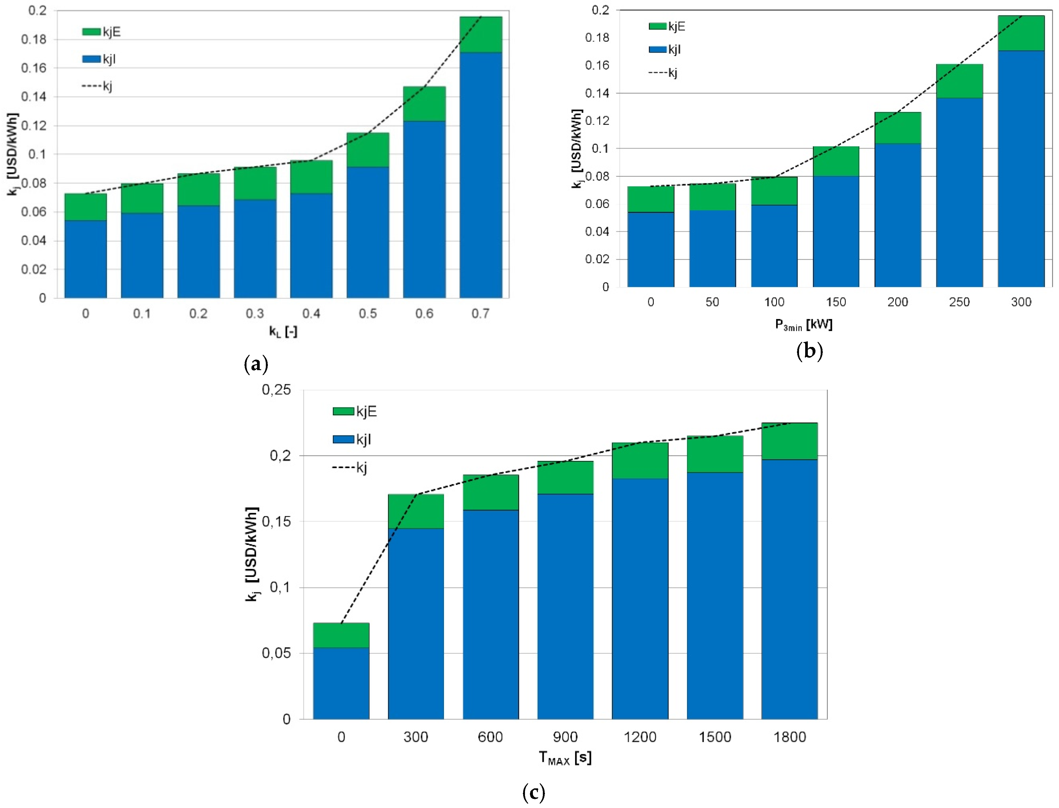
Figure 8 and Figure 9 show the results on calculations of variation in the unit cost of optimal solutions as a function of the three characteristic parameters of the WPP-FESS system: the index of elimination of allowable interruptions k_L (Figure 8a and Figure 9a), the minimum power at the output of the WPP-FESS system P_3MIN (Figure 8b and Figure 9b) and time T_MAX (Figure 8c and Figure 9c) for the measurement data for 2011 and 2012. In the completed analyses, the k_L index varies from 0 to 0.7 in steps of 0.1; the output of P_3MIN range from 0 kW to 300 kW in steps of 50 kW. T_MAX was changed from 0 s to 1800 s with a step of 300 s. In all figures, the division of the unit cost of k_j (dashed line) into the investment (k_jI) and operational (k_jE) components was taken into account—refer to the bar charts.

Based on the obtained results (Figure 4, Figure 5, Figure 6, Figure 7, Figure 8 and Figure 9, Table 1), it should be stated that the main component of the discounted unit cost of electricity generation in the analysed systems are investment costs representing 72 to 75% of the total cost. Significant changes in the k_j cost as a function of the three aforementioned parameters used in the algorithm of interface of the WPP-FESS system with the power grid are noticeable: k_L interval elimination index, P_3MIN power and T_MAX time. The mentioned changes are non-linear in nature and convergent for all wind speed data analysed in the paper.

Dependences k_j = f(k_L)—Figure 8a and Figure 9a—and k_j = f(P_3MIN)—Figure 8b and Figure 9b are characterised, in the analysed geographical location, by a strong increase in unit energy generation cost for k_L > 0.5 and P_3MIN > 10%P_WPPn. Based on the results shown in Figure 8c and Figure 9c (dependence k_j = f(T_MAX)), it can be concluded that for all analysed years and locations under consideration, the cost value k_j stabilises for T_MAX times between 1500 s and 1800 s. On the basis of studies conducted in [6], this is a feature specific for this geographical location and local wind conditions. The limit values of T_MAX time will, therefore, depend on these factors. The number of interruptions longer than mentioned above is small in comparison with shorter interruptions, so if the ratio of allowed interruptions k_L is adopted at a certain assumed level, e.g., 0.7, it is possible to eliminate a significant part of them. This is evidenced by the lower increase in the dependence of the unit cost of energy generation as a function of T_MAX time.

Detailed results comparing the percentage increase in the unit cost of electricity generation Δk_j% for the optimised WPP-FESS system in relation to an identical wind power plant without energy storage as a function of the tested system parameters and the two considered years 2011 and 2012 are presented in

Table 2. Increase in the unit cost of electricity generation Δk_j% for an optimised wind power plant–energy storage system (WPP-FESS system with the power rating of 2 MW compared to an optimised system without energy storage for different values of k_L, P_3MIN and T_MAX.

kL [–]	Δkj%		P3MIN [kW]	Δkj%		TMAX [s]	Δkj%
	2011	2012		2011	2012		2011	2012
0.1	9%	9%	50	18%	3%	300	82%	134%
0.2	18%	19%	100	21%	9%	600	165%	154%
0.3	23%	25%	150	29%	39%	900	172%	169%
0.4	29%	32%	200	63%	73%	1200	189%	188%
0.5	50%	58%	250	113%	121%	1500	192%	195%
0.6	93%	102%	300	172%	169%	1800	205%	209%
0.7	172%	169%	–	–	–	–	–	–

. Attention should be paid to the values highlighted in grey, which significantly increase the actual cost of energy generation in the WPP-FESS system compared to the wind power plant without an energy storage system.

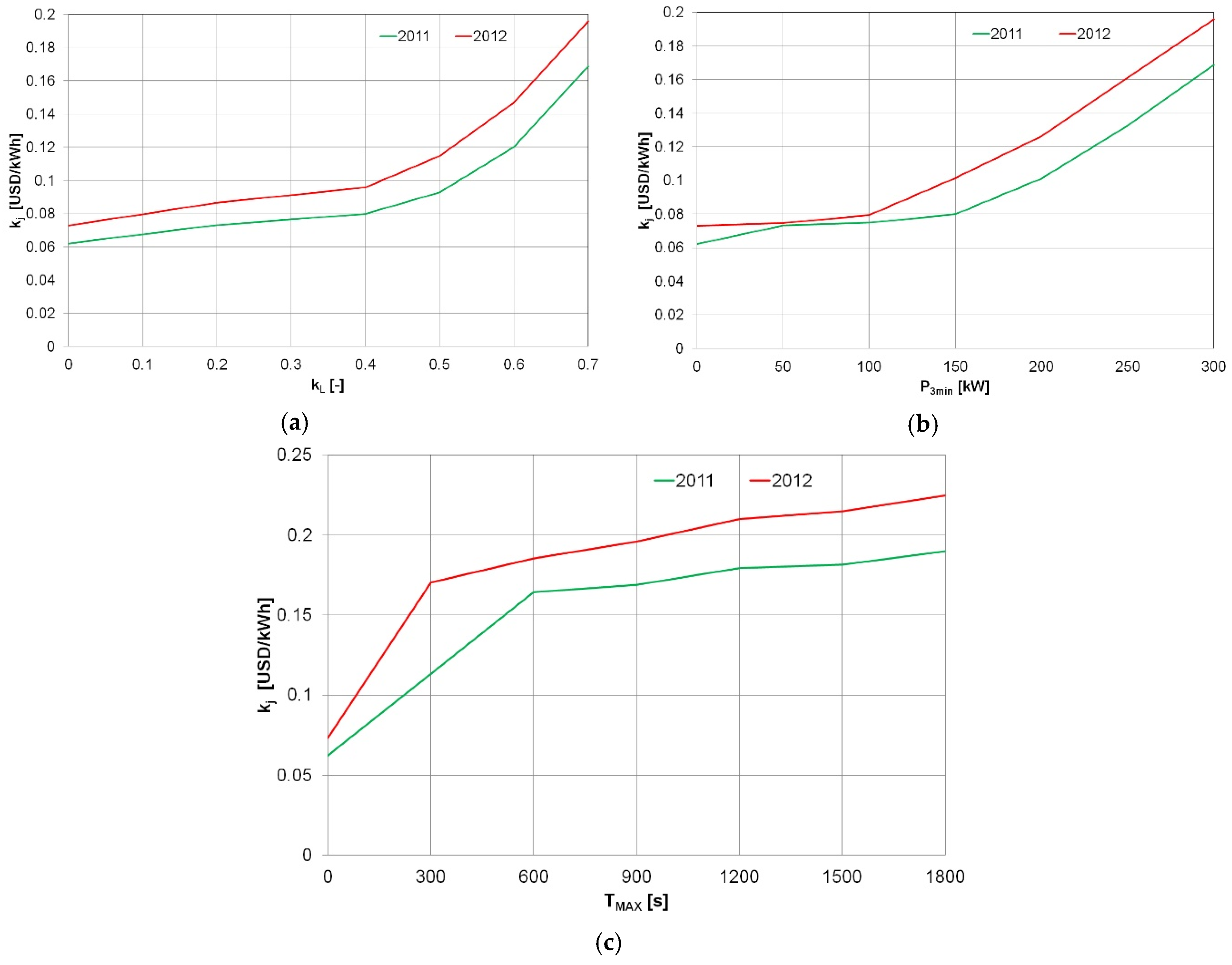
In addition, important conclusions can be drawn from the comparison of the nature and changes of the cost k_j as a function of the k_L, P_3MIN and T_MAX parameters for wind data for 2011 and 2012, presented in Figure 10.

On the basis of the breakdown of results (Figure 10), significant differences were found in the level of unit costs of electricity generation in optimised WPP-FESS systems for wind conditions close to the average for 2008–2012 (2011) and for the worst conditions (2012). These differences depend on the value of the considered parameter and assume values from 15 to 28%. On this basis, it can be concluded that the optimisation analyses conducted in the article should be carried out for years with worse wind conditions, and the obtained solutions will help in meeting the assumed conditions of interface of the WPP-FESS system with the power grid.

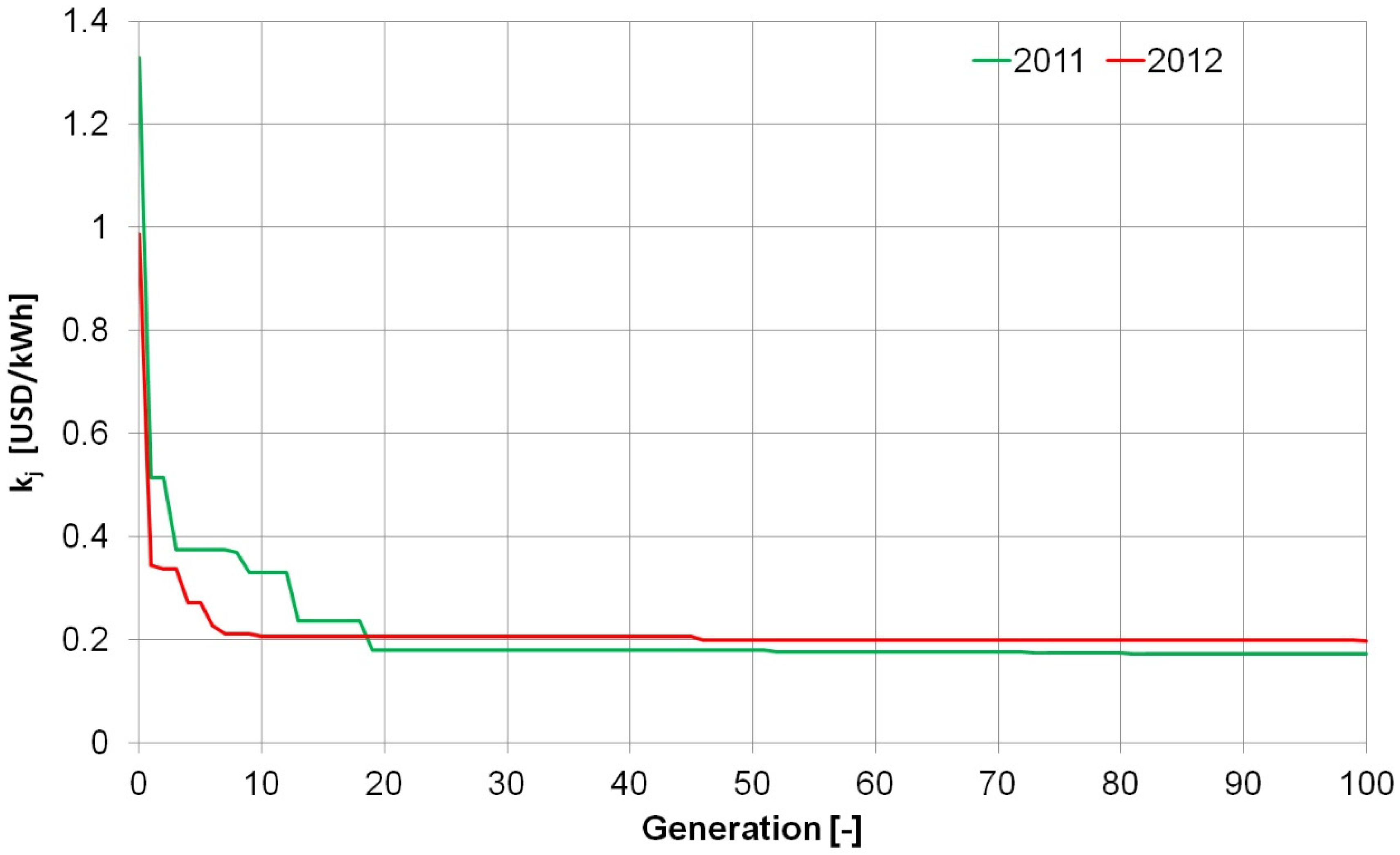
In order to demonstrate the high efficiency of the genetic algorithm used for optimisation, Figure 11 λ shows the evolution of the best individual quality index as a function of generation number for two optimisation tasks in 2011 and 2012 for which k_L = 0.7, T_MAX = 1800 s, P_3MIN = 300 kW. In both cases, the optimisation method used shows good convergence, which results in stabilisation of the solution after only about 40–50 generations. The analysis of the characteristics of other cases has shown that the latest corrections to the optimal solution are obtained between the 70th and 90th generation. On this basis, the authors determined the number of generations of the applied genetic algorithm equal to 100. Monotonous reduction of the fit function value is related to the application of an elite strategy in the developed algorithm.

6. Conclusions

The paper presents an original algorithm for reducing the discounted unit cost of electricity generation k_j using the UNIPEDE method (used to compare various power industry facilities) in the systems of wind power plants interfacing with flywheel energy storage systems. The purpose of using flywheel energy storage systems is to improve the quality and stability of supply from power plants to the power grid. The objective is achieved by reducing the number of periods (with duration up to T_MAX) of reduced capacity supplied from the power plant to the power grid in relation to the reference value of P_3MIN.

In order to achieve the described objective, the method of modified (by the authors) genetic algorithm, a developed model of the system (wind power plant and flywheel energy storage) and implemented control system for the operation of the storage system depending on the current state of wind energy, turbine and energy storage system were applied. The applied system model and optimisation method enabled the authors to determine the values of the minimum cost of electricity generation in the analysed system as a function of three system parameters and the energy flow control system from and to the storage system: k_L interval elimination index, P_3MIN reference power and T_MAX time.

The combination of a wind power plant with energy storage systems raises the unit costs of electricity generation in relation to the system consisting only of a wind power plant. Based on the analysis of the obtained results, it was found that the percentage increase in the unit cost of electricity generation Δk_j% for the optimised WPP-FESS system in relation to optimised wind power plants without energy storage is strongly dependent on the year of analysis and the adopted values of the allowable interruption index k_L, P_3MIN power and T_MAX time. Its value varies from several to over 200% for the maximum values of T_MAX = 1800 s, P_3MIN = 300 kW and k_L = 0.7. The provided range of the increase in the k_j cost requires a detailed comparative analysis of the obtained effects (improvement of the indices of energy supply to the power grid and the related restriction of penalties for failure to meet the required conditions of power supply, particularly to large industrial consumers, strategic for security) and the actual cost of the system.

On the basis of the research conducted for the selected geographical location (established wind conditions), it can be concluded that the best values of the coefficients in question are: P_3MIN = 10% P_WPPn and k_L = 0.5, for which the increase in the cost of the WPP-FESS system in relation to the system without energy storage does not exceed 73%.

References

- Liu, H.; Li, D.; Liu, Y.; Dong, M.; Liu, X.; Zhang, H. Sizing Hybrid Energy Storage Systems for Distributed Power Systems under Multi-Time Scales. Appl. Sci. 2018, 8, 1453. [Google Scholar] [CrossRef]
- Norshahrani, M.; Mokhlis, H.; Bakar, H.; Jamian, J.J.; Sukumar, S. Progress on Protection Strategies to Mitigate the impact of Renewable Distributed Generation on Distribution Systems. Energies 2017, 10, 1864. [Google Scholar] [CrossRef]
- Wang, Z.; Luo, D.; Li, R.; Zhang, L.; Liu, C.; Tian, X.; Li, Y.; Su, Y.; He, J. Research on the active power coordination control system for wind/photovoltaic/energy storage. In Proceedings of the 2017 1st IEEE Conference on Energy Internet and Energy System Integration, Beijing, China, 26–28 November 2017; pp. 1–5. [Google Scholar]
- Telukunta, V.; Pradhan, J.; Agrawal, A.; Singh, M.; Srivani, G.S. Protection challenges under bulk penetration of renewable energy resources in power systems: A review. CSEE J. Power Energy Syst. 2017, 3, 365–379. [Google Scholar] [CrossRef]
- Guezgouz, M.; Jurasz, J.; Bekkouche, B. Techno-Economic and Enviromental Analysis of a Hybrid PV-WT-PSH/BB Standalone System Supplying Various Loads. Energies 2019, 12, 514. [Google Scholar] [CrossRef]
- Tomczewski, A. Operation of a Wind Turbine-Flywheel Energy Storage System under Conditions of Stochastic Change of Wind Energy. Sci. World J. 2014, 2014, 643769. [Google Scholar] [CrossRef] [PubMed]
- Liang, X. Emerging Power Quality Challenges Due to Integration of Renewable Energy Sources. IEEE Trans. Ind. Appl. 2017, 53, 855–866. [Google Scholar] [CrossRef]
- Díaz-Gonzáleza, F.; Sumpera, A.; Gomis-Bellmunta, O.; Villafáfila-Roblesb, R. A review of energy storage technologies for wind power applications. Renew. Sustain. Energy Rev. 2012, 16, 2154–2171. [Google Scholar] [CrossRef]
- Fuchs, G.; Lunz, B.; Leuthold, M.; Sauer, D.U. Technology Overview on Electricity Storage; Overview on the Potential and on the Deployment Perspectives of Electricity Storage Technologies; Institute for Power Electronics and Electrical Drives: Aechen, Germany, 2012. [Google Scholar]
- Kasprzyk, L. Modelling and analysis of dynamic states of the lead-acid batteries in electric vehicles. Eksploat. Niezawodn. 2017, 19, 229–236. [Google Scholar] [CrossRef]
- Barelli, L.; Bidini, G.; Bonucci, F.; Castellini, L.; Castellini, S.; Ottaviano, A.; Pelosi, D.; Zuccari, A. Dynamic Analysis of a Hybrid Energy Storage System (H-ESS) Coupled to a Photovoltaic (PV) Plant. Energies 2018, 11, 396. [Google Scholar] [CrossRef]
- Amiryar, M.E.; Pullen, K.R. A Review of Flywheel Energy Storage System Technologies and Their Applications. Appl. Sci. 2017, 7, 286. [Google Scholar] [CrossRef]
- Nguyen, T.T.; Yoo, H.J.; Kim, H.M. A Flywheel Energy Storage System Based on a Doubly Fed Induction Machine and Battery for Microgrid Control. Energies 2015, 8, 5074–5089. [Google Scholar] [CrossRef]
- Tomczewski, A.; Kasprzyk, L. Optimisation of the Structure of a Wind Farm-Kinetic Energy Storage for Improving the Reliability of Electricity Supplies. Appl. Sci. 2018, 8, 1439. [Google Scholar] [CrossRef]
- Chudy, M.; Herbst, L.; Lalk, J. Wind farms associated with flywheel energy storage plants. In Proceedings of the IEEE PES Innovative Smart Grid Technologies, Europe, Istanbul, Turkey, 12–15 October 2014. [Google Scholar]
- Moualdia, A.; Medjber, A.; Kouzou, A.; Bouchhida, O. DTC-SVPWM of an energy storage flywheel associated with a wind turbine based on the DFIM. Sci. Iran. 2018, 25, 3532–3541. [Google Scholar] [CrossRef]
- Diaz-Gonzalez, F.; Bianchi, F.D.; Sumper, A.; Gomis-Bellmunt, O. Control of a Flywheel Energy Storage System for Power Smoothing in Wind Power Plants. IEEE Trans. Energy Convers. 2014, 29, 204–214. [Google Scholar] [CrossRef]
- Mir, A.S.; Senroy, N. Intelligently Controlled Flywheel Storage for Wind Power Smoothing. In Proceedings of the 2018 IEEE Power & Energy Society General Meeting (PESGM), Portland, OR, USA, 5–10 August 2018. [Google Scholar]
- Ghosh, S.; Kamalasadan, S. An Energy Function-Based Optimal Control Strategy for Output Stabilization of Integrated DFIG-Flywheel Energy Storage System. IEEE Trans. Smart Grid 2017, 8, 1922–1931. [Google Scholar] [CrossRef]
- Lai, J.; Song, Y.; Du, X. Hierarchical Coordinated Control of Flywheel Energy Storage Matrix Systems for Wind Farms. IEEE-ASME Trans. Mechatron. 2018, 23, 48–56. [Google Scholar] [CrossRef]
- Jauch, C. Controls of a flywheel in a wind turbine rotor. Wind Eng. 2016, 40, 173–185. [Google Scholar] [CrossRef]
- Sebastian, R.; Pena-Alzola, R. Control and simulation of a flywheel energy storage for a wind diesel power system. Int. J. Electr. Power Energy Syst. 2015, 64, 1049–1056. [Google Scholar] [CrossRef]
- Ding, Y.; Wang, P.; Chang, L.P. Reliability evaluation of electric power system with high wind power penetration. In Proceedings of the 2009 8th International Conference on Reliability, Maintainability and Safety, Chengdu, China, 20–24 July 2009; pp. 24–26. [Google Scholar]
- Mohamad, F.; The, J.; Lai, C.M.; Chen, L.R. Development of Energy Storage Systems for Power Network Reliability: A Review. Energies 2018, 11, 2278. [Google Scholar] [CrossRef]
- Glossary of Terms Used in Reliability Standards; NERC: Swindon, UK, 2008.
- Power System Reliability Analysis; Application Guide; CIGRE WG 03 of SC 38 (Power System Analysis and Techniques); e-cigre: Paris, France, 1987.
- Power System Reliability Analysis; Composite Power System Reliability Evaluation; CIGRE Task Force 38-03-10; e-cigre: Paris, France, 1992.
- Wen, S.; Lan, H.; Fu, Q.; Yu, D.C.; Zhang, L. Economic Allocation for Energy Storage System Considering Wind Power Distribution. IEEE Trans. Power Syst. 2015, 30, 644–652. [Google Scholar] [CrossRef]
- Lakshminarayana, S.; Xu, Y.; Poor, V.H.; Quek, S.Q.T. Cooperation of Storage Operation in a Power Network with Renewable Generation. IEEE Trans. Smart Grid 2016, 7, 2108–2122. [Google Scholar] [CrossRef]
- Tomczewski, A. Techniczno-Ekonomiczne Aspekty Optymalizacji Wybranych Układów Elektrycznych, 1st ed.; Wydawnictwo Politechniki Poznanskiej: Poznan, Poland, 2014; ISBN 978-83-7775-332-3. [Google Scholar]
- Kaabeche, A.; Belhamel, M.; Ibtiouen, R. Techno-economic valuation and optimization of integrated photovoltaic/wind energy conversion system. Sol. Energy 2011, 85, 2407–2420. [Google Scholar] [CrossRef]
- Kasprzyk, L.; Tomczewski, A.; Bednarek, K. Efficiency and economic aspects in electromagnetic and optimization calculations of electrical systems. Prz. Elektrotech. 2010, 86, 57–60. [Google Scholar]
- Komarnicki, P.; Lombardi, P.; Styczynski, Z. Economics of Electric Energy Storage Systems. In Electric Energy Storage Systems; Springer: Berlin/Heidelberg, Germany, 2017; pp. 181–194. [Google Scholar]
- Mohammed, H.O.; Amirat, Y.; Benbouzid, M. Economical Evaluation and Optimal Energy Management of a Stand-Alone Hybrid Energy System Handling in Genetic Algorithm Strategies. Electronics 2018, 7, 233. [Google Scholar] [CrossRef]
- Cheng, S.; Sun, W.B.; Liu, W.L. Multi-Objective Configuration Optimization of a Hybrid Energy Storage System. Appl. Sci. 2017, 7, 163. [Google Scholar] [CrossRef]
- Bednarek, K.; Nawrowski, R.; Tomczewski, A. An application of genetic algorithm for three phases screened conductors optimization. In Proceedings of the 2000 International Conference on Parallel Computing in Electrical Engineering, Trois-Rivieres, QC, Canada, 27–30 August 2000; pp. 218–222. [Google Scholar]
- Kasprzyk, L.; Nawrowski, R.; Tomczewski, A. Optimization of Complex Lighting Systems in Interiors with use of Genetic Algorithm and Elements of Paralleling of the Computation Process. In Intelligent Computer Techniques in Applied Electromagnetics; Studies in Computational Intelligence; Wiak, S., Krawczyk, A., Dolezel, I., Eds.; Springer: Berlin/Heidelberg, Germany; New York, NY, USA, 2008; Volume 116, pp. 21–29. [Google Scholar]
- Kaviani, A.; Baghaee, H.R.; Riahy, G.H. Optimal sizing of a stand-alone wind/photovoltaicgeneration unit using particle swarm optimization. Simul. Trans. Soc. Model. Simul. 2009, 85, 89–99. [Google Scholar]
- Alemany, J.; Kasprzyk, L.; Magnago, F. Effects of binary variables in mixed integer linear programming based unit commitment in large-scale electricity markets. Electr. Power Syst. Res. 2018, 160, 429–438. [Google Scholar] [CrossRef]
- Castro Mora, J.; Calero Baro, J.M.; Riguelme Santos, J.M.; Burgos Payan, M. An evolutive algorithm for wind farm optimal design. Neurocomputing 2007, 70, 2651–2658. [Google Scholar] [CrossRef]
- Goldberg, D.E. Genetic Algorithms in Search, Optimization and Machine Learning; Addison-Wesley Longman Publishing: Boston, MA, USA, 1988. [Google Scholar]
- Michalewicz, Z.; Fogel, D.B. How to Solve It; Modern Heuristics, 2nd ed.; Springer: Berlin/Heidelberg, Germany, 2004. [Google Scholar]
- Baeck, T.; Fogel, D.B.; Michalewicz, Z. Hanbook of Evolutionary Computation, Penalty Functions; IOP Publishing and Oxford University Press: London, UK, 1997. [Google Scholar]
- Blicke, T.; Thiele, L. A Comparison of Selection Schemes used in Genetic Algorithms; TIK-Report; Computer Engineering and Communication Networks Lab, Swiss Federal Institute of Technology: Zurich, Switzerland, 1995. [Google Scholar]
- Sztuba, W.; Horodko, K.; Ratajczak, M.; Kajetanowicz, K.; Palusinski, M.; Czarnecka, B.; Prusak, M.; Soltysiak, D.; Lesniewski, L. Wind Energy in Poland; TPA Horwath: Poland, 2012. [Google Scholar]
- Akhil, A.A.; Huff, G.; Currier, B.A.; Kaun, C.B.; Rastler, M.D.; Chen, B.S.; Cotter, L.A.; Bradshaw, T.D.; Gauntlett, D.W. DOE/EPRI Electricity Storage Handbook in Collaboration with NRECA; Sandia National Laboratories: Albuquerque, NM, USA; Livermore, CA, USA, 2015.
Figure 1.
(a) Electrical diagram and power flow directions in the wind power plant–energy storage system (WPP-FESS) arrangement (PWT1, PWT2, …, PWTN—capacity of wind turbines in the power plant, PWPPn—rated capacity of the wind power plant, PFESSn—rated capacity of the storage system, P1(t), P2(t), P3(t)—active capacity of the power plant, storage system and delivered to the grid at moment t, respectively, AFESSn—rated capacity of the storage system); (b) the connection structure of the FESS module group.
Figure 2.
Block diagram of the interface algorithm between the flywheel storage system and the wind power plant.
Figure 3.
Block model of the application designed to optimise the wind power plant-flywheel energy storage system arrangements (W1, W2, …, WNwp are logical processors used in the process of paralleling).
Figure 4.
Value of discounted unit cost kj of energy generation in an optimised WPP system without energy storage.
Figure 5.
Increase in the value of discounted unit cost kj of energy generation in an optimised WPP system without energy storage with reference to the year with best wind conditions.
Figure 6.
Values of: (a) mean wind speed, (b) energy generated over a period of one year in an optimised power plant layout without energy storage, as a function of the analysed years.
Figure 7.
Values of the discounted unit cost of energy production in the optimised WPP-FESS system as a function of the ratio of elimination of allowable interruptions kL for 2008, 2011 and 2012.
Figure 8.
Values of the discounted unit cost of energy generation in the optimised WPP-FESS system for the year 2011 as a function of: (a) index of elimination of acceptable interruptions kL (P3MIN = 300 kW, TMAX = 900 s); (b) P3MIN power (TMAX = 600 s, kL = 0.7), (c) time TMAX (P3MIN = 300 kW, kL = 0.7).
Figure 9.
Values of the discounted unit cost of energy generation in the optimised WPP-FESS system for the year 2012 as a function of: (a) index of elimination of acceptable interruptions kL (P3MIN = 300 kW, TMAX = 900 s); (b) P3MIN power (TMAX = 600 s, kL = 0.7), (c) time TMAX (P3MIN = 300 kW, kL = 0.7).
Figure 10.
Comparison of the value of the discounted unit cost of energy generation in the optimised WPP-FESS system in 2011 and 2012 as a function of: (a) allowable interruption index kL (P3MIN = 300 kW, TMAX = 900 s); (b) P3MIN power (TMAX = 900 s, kL = 0.7); (c) TMAX time (P3MIN = 300 kW, kL = 0.7).
Figure 11.
Evolution of the best individual quality index as a function of generation number for two optimisation tasks in 2011 and 2012 for which kL = 0. 7, TMAX = 1800 s, P3MIN = 300 kW.