Multi-Step-Ahead Carbon Price Forecasting Based on Variational Mode Decomposition and Fast Multi-Output Relevance Vector Regression Optimized by the Multi-Objective Whale Optimization Algorithm

Abstract

The accurate and stable forecasting of carbon prices is vital for governors to make policies and essential for market participants to make investment decisions, which is important for promoting the development of carbon markets and reducing carbon emissions in China. However, it is challenging to improve the carbon price forecasting accuracy due to its non-linearity and non-stationary characteristics, especially in multi-step-ahead forecasting. In this paper, a hybrid multi-step-ahead forecasting model based on variational mode decomposition (VMD), fast multi-output relevance vector regression (FMRVR), and the multi-objective whale optimization algorithm (MOWOA) is proposed. VMD is employed to extract the primary mode for the carbon price. Then, FMRVR, which is used as the forecasting module, is built on the preprocessed data. To achieve high accuracy and stability, the MOWOA is utilized to optimize the kernel parameter and input the lag of the FMRVR. The proposed hybrid forecasting model is applied to carbon price series from three major regional carbon emission exchanges in China. Results show that the proposed VMD-FMRVR-MOWOA model achieves better performance compared to several other multi-output models in terms of forecasting accuracy and stability. The proposed model can be a potential and effective technique for multi-step-ahead carbon price forecasting in China’s three major regional emission exchanges.

1. Introduction

Global climate change induced by greenhouse emissions has become a serious challenge to the sustainable development of society, which has attracted worldwide attention recently. An emission trading scheme as an effective market mechanism to reduce carbon emission is widely applied worldwide [1]. The additional cost of excess emissions mitigates companies’ motivation for excessive production and stimulates them to seek a more green production approach, which results in overall carbon emission mitigation. China is the largest carbon emitter [2,3,4], accounting for 28% of the world emissions [5] in 2015, and reaching 10,433 Mton CO₂ emission eq/yr (equivalent per year) in 2016 [6]. In response to the challenge of global warming, China has established eight pilot regional emission exchanges in Shenzhen, Guangdong, Hubei, Tianjin, Shanghai, Chongqing, Beijing, and Fujian since 2013 [2,7]. Accurate carbon price forecasting is not only critical for governors to make policies [3] but also important for the reasonable production arrangement of carbon emission companies to reduce costs and increase profit. Additionally, it is vital for investors to mitigate price risk and maximize investment revenue [8]. However, carbon prices are impacted by both the external environmental variation [9] and investors’ heterogeneous beliefs, which makes carbon prices non-stationary and non-linear. Therefore, promoting the accuracy of carbon price forecasting is a challenge for academics and an important topic in the field of energy policy and energy consumption.

Accurate carbon price forecasting has attracted extensive attention worldwide. Recent studies on carbon price series forecasting can be divided into three categories: econometrics models, artificial intelligence models, and hybrid (ensemble) models. The first category includes multiple linear regression [10], generalized autoregressive conditional heteroskedasticity (GARCH) [11], and heterogeneous autoregressive with realized volatility (HAR-RV) models [12]. The limitation in econometric models is the difficulty in dealing with the non-linearity of a carbon price series. To overcome such limitations, artificial intelligence models are applied widely in carbon price series forecasting, such as the least square support vector machine (LSSVM) method [13], multi-layered perceptron (MLP)-artificial neural network (ANN) model [14]. The hybrid model shows better performance compared to a single model in time series forecasting [15,16,17,18]. To further improve the forecasting performance in carbon price forecasting, the hybrid (ensemble) models are proposed. Sun et al. [19] proposed a combined variational mode decomposition (VMD)-spiking neural network (SNN) model to forecast carbon price from Intercontinental Exchange (ICE). Zhou et al. [20] proposed a multiscale ensemble model based on ensemble empirical mode decomposition (EEMD), extreme learning machine (ELM), and support vector machine (SVM) models to forecast carbon price in the Shenzhen Emissions Exchange. Zhu et al. [1] proposed a novel ensemble model based on empirical mode decomposition (EMD) and LSSVM with a kernel function prototype for ICE carbon price forecasting. Zhu et al. [3] proposed a multiscale ensemble model based on EMD and the evolutionary least squares support vector regression for carbon price forecasting in the European Climate Exchange. Zhu and Wei [21] proposed a novel hybrid model based on autoregressive integrated moving average model (ARIMA) and LSSVM to forecast two main carbon future prices from the European Climate Exchange. Atsalakis [22] proposed a computational intelligence technique called PATSOS (a forecasting model consisted of two ANFIS models) based on two adaptive neuro-fuzzy inference system (ANFIS) sub-systems to manage the risk in carbon price trading in the European Energy Exchange.

In general, the hybrid method achieves better performance in carbon price forecasting [1,3,19,20,21,22]. However, there are three deficiencies which exist in recent studies: (1) Existing studies focus on the one-step forecasting of carbon price series, and few studies focus on multi-step forecasting which is important to allow market participants to make more long-term decisions. (2) Most existing studies focus on the carbon price in the European market. Few studies have paid attention to carbon price series in carbon emission exchanges in China. However, as the largest carbon emitter worldwide, studies on Chinese carbon emission exchanges are of significance. (3) The existing ANN and SVR methods can’t provide probabilistic forecasting (i.e., variance in the forecasted value) without additional computation. To compensate for the above gaps and promote the accuracy in multi-step-ahead carbon price forecasting, we propose a hybrid multi-step-ahead forecasting model based on VMD, fast multi-output relevance vector regression (FMRVR), and the multi-objective whale optimization algorithm (MOWOA) for carbon price series from three major carbon emission exchanges in China.

The proposed hybrid multi-step-ahead forecasting model VMD-FMRVR-MOWOA contains three modules. First, the VMD is used as the preprocessing module to eliminate persistent noise in the price series. Then, the FMRVR, which is utilized as the forecasting module is estimated based on the preprocessed data. Finally, the MOWOA is applied to optimize the kernel parameter and input lag for the FMRVR to obtain better performance. The proposed model is applied to three carbon prices from three major pilot regional emission exchanges in China: Shenzhen emission allowance 2016 (SZA2016), Guangdong emission allowance (GDEA), and Hubei emission allowance (HBEA). The results show that the proposed method achieves better performance compared to other multi-output models. The main contributions of our study are as follows: (a) FMRVR is used to forecast carbon price for the first time. (b) MOWOA is used to optimize the FMRVR for the first time. (c) As far as we know, the proposed VMD-FMRVR-MOWOA is the first multi-step-ahead forecasting model applied to carbon price series. (d) The carbon price series from three major regional emission exchanges in China are analyzed.

The remainder of this paper is organized as follows: Section 2 describes the framework of the proposed model and presents a brief description of VMD, FMRVR, and MOWOA, respectively. Section 3 introduces a case study of three major regional emissions exchanges in China and analyses the results. Section 4 concludes our study.

2. Materials and Methods

2.1. The Proposed Method

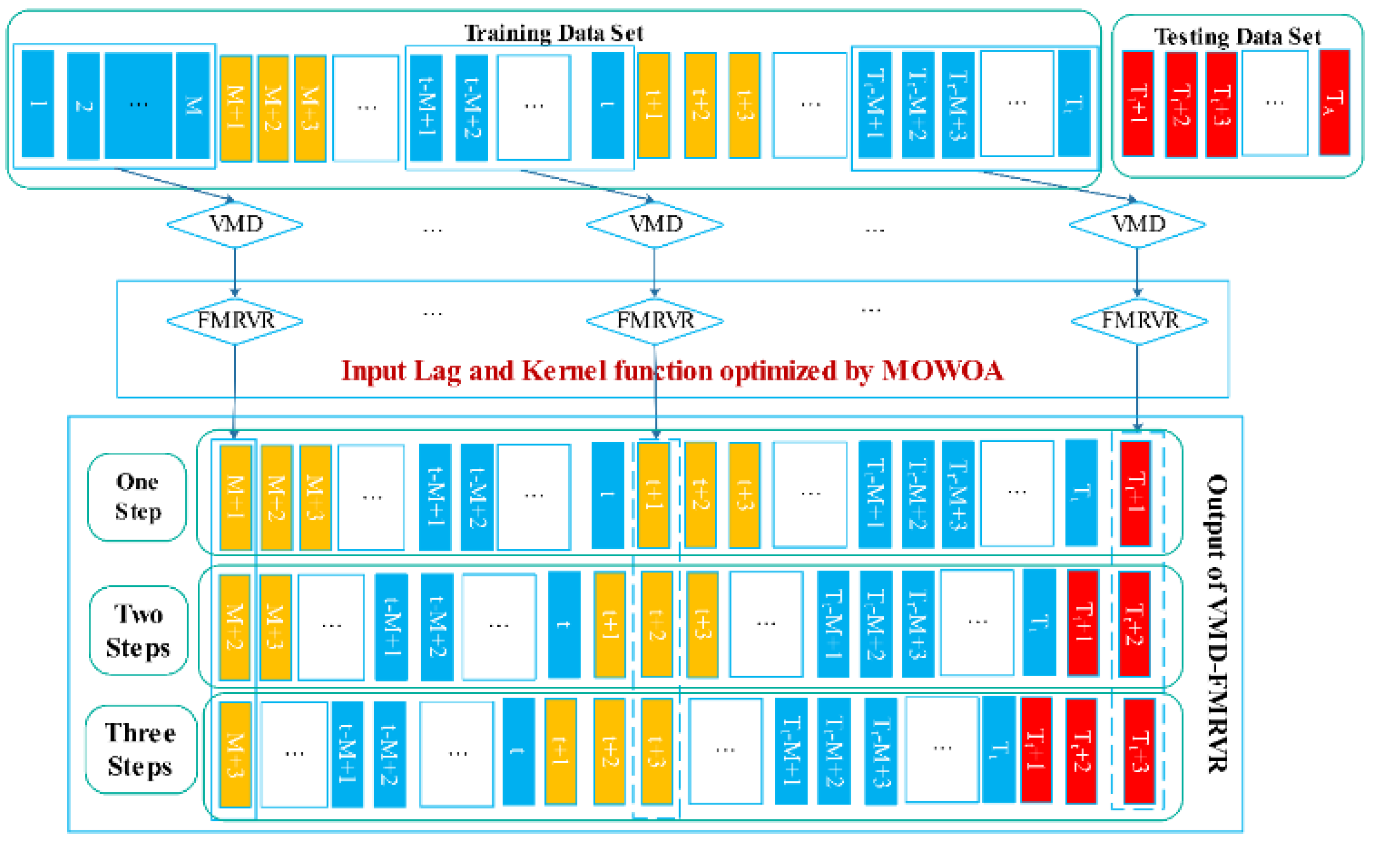
The proposed model VMD-FMRVR-MOWOA contains three modules. (1) Preprocessing module: For non-linear and non-stationary characteristics [9], the carbon price is often preprocessed to extract the main mode hidden in the series. EMD and VMD are two commonly used methods [1,23,24,25]. VMD is used to denoise the original series in our study since VMD demonstrates better noise robustness than EMD [26]. (2) Forecasting module: FMRVR is applied as the multi-step forecasting module of the proposed model. The RVR, which is a Bayesian learning method using the kernel-trick, is applied widely in time series analysis [27,28,29,30,31,32] because it has significant advantages of sparsity formulation and probabilistic output, the ability to use non-Mercer kernels but only one output. Thayananthan, et al. [33] extended RVM to multi-output relevance vector regression (MRVR); however, it still has the limitation of low computational efficiency. The FMRVR used in this paper is a fast version of the MRVR proposed by Ha [34]. The kernel parameter and input lag are crucial in the use of FMRVR. (3) Optimization module: MOWOA, which is an efficient meta-heuristic multi-objective optimization algorithm, is applied to optimize these two parameters. Multi-step-ahead forecasting needs to compare multi-objective performance simultaneously; thus, the multi-objective optimization method is essential [35,36,37,38]. As MOWOA achieves better performance than two recently developed algorithms (i.e., multi-objective ant lion optimization algorithm (MOALO) and multi-objective dragonfly algorithm (MODA)) [39], it is chosen as the optimization method in this study.

The structure of the hybrid model is shown in Figure 1. The whole data set is split into two parts: training set and test set. The proposed method consists of five main steps.

Step 1:

setting a moving window (window length equal to M) to select the input data for the VMD-FMRVR models.

Step 2:

denoising the data series in the fixed number window by VMD to obtain the denoised data series.

Step 3:

estimating the parameters in FMRVR based on the denoised data series in the given window and then forecasting to obtain the values of the three steps beyond the given window. The input lags and width of the kernel function in FMRVR module are randomly given.

Step 4:

repeating VMD-FMRVR modeling with the movement of the window.

Step 5:

finding the best input lags and width of the kernel function in the FMRVR by the MOWOA.

2.2. Modules in Proposed Model

2.2.1. Variational Mode Decomposition (VMD)

The VMD algorithm is a signal decomposition technique proposed by Dragomiretskiy and Zosso [40], which decomposes the original signal into K intrinsic mode functions (IMFs). The key idea of VMD in obtaining the final K IMFs is to minimize the bandwidth sum of the IMFs. To obtain the mode bandwidth, three steps are applied:

(1)

Obtaining the unilateral frequency spectrum of each mode $u_k$ by a Hilbert transformation.

$$\left(\delta \left(t\right)+\frac{j}{\pi t}\right)\times u_k\left(t\right)$$

(1)

(2)

Shifting the mode’s frequency spectrum to “baseband”

$$\left[\left(\delta \left(t\right)+\frac{j}{\pi t}\right)\times u_k\left(t\right)\right]e^{-j{\omega }_{k}t}$$

(2)

(3)

Estimating the bandwidth by the H1 Gaussian smoothness. The decomposition process is realized by solving the following optimization problem [22]:

$$\begin{array}{l}\underset{\left\{u_k\right\},\left\{{\omega }_k\right\}}{{\displaystyle \min }}\left\{{\displaystyle \sum _k{\Vert {\partial }_t\left[\left(\delta \left(t\right)+\frac{j}{\pi t}\right)\times u_k\left(t\right)\right]e^{-j{\omega }_{k}t}\Vert }_2^2}\right\}\\ s.t.{\displaystyle \sum _k{u}_k}=s\end{array}$$

(3)

where $\left\{u_k\right\}=\left\{u_1,u_2,\cdots ,u_K\right\}$ are the modes, $\left\{{\omega }_k\right\}=\left\{{\omega }_1,{\omega }_2,\cdots ,{\omega }_K\right\}$ are the center frequencies of the modes. $\delta \left(t\right)$ is the Dirac function, and $*$ is the convolution operation. $s$ is the original signal. The alternate direction method of multipliers (ADMM) is used to solve the above optimization problem. The complete algorithm of ADMM for obtaining the final parameters and modes in VMD is shown in Figure 2 (modified based on Dragomiretskiy’s pseudo-code [40]).

2.2.2. Fast Multi-Output Relevance Vector Regression (FMRVR)

The RVM, which was invented by Tipping [41], is used for multi-input but single-output regression. Thayananthan [42] and Thayananthan et al. [33] extended the RVM to the MRVR, which has the limitation of low computational efficiency. To overcome this limitation, Ha [34] proposed the FMRVR to decrease the time complexity of the MRVR.

Model Specification of the FMRVR

Given a data set of input-output pairs ${\left\{{\mathrm{x}}_i\in {ℝ}^{U\times 1},{\mathrm{t}}_i\in {ℝ}^{1\times V}\right\}}_{i=1}^N$, a V-dimensional multi-output U-dimensional input regression can be expressed as follows:

$${\mathrm{t}}_i=y\left({\mathrm{x}}_i;\mathrm{W}\right)+{\epsilon }_i$$

(4)

where $\mathrm{W}\in {ℝ}^{\left(\mathrm{N}+1\right)\times \mathrm{V}}$ is the weight matrix, and ${\epsilon }_i\in {ℝ}^{1\times \mathrm{V}}$ is the noise vector. $y\left({\mathrm{x}}_i;\mathrm{W}\right)$ = $\left[1\hspace{0.17em}K\left({\mathrm{x}}_i{,\mathrm{x}}_1\right)\hspace{0.17em}K\left({\mathrm{x}}_i{,\mathrm{x}}_2\right)\hspace{0.17em}\cdots \hspace{0.17em}K\left({\mathrm{x}}_i{,\mathrm{x}}_{\mathrm{N}}\right)\right]\mathrm{W}$. $K\left({\mathrm{x},\mathrm{x}}^{\prime }\right)$ is a kernel function. The U-input V-output model can be also expressed as follows:

$$\mathrm{T}=\mathsf{\Phi }\mathrm{W}+\mathrm{E}$$

(5)

where $\mathrm{T}={\left[{\mathrm{t}}_1\hspace{0.17em}{\mathrm{t}}_2\hspace{0.17em}\cdots \hspace{0.17em}{\mathrm{t}}_{\mathrm{N}}\right]}^{\mathrm{T}}\in {ℝ}^{\mathrm{N}\times \mathrm{V}}$, $\mathsf{\Phi }={\left[\varphi \left({\mathrm{x}}_1\right)\hspace{0.17em}\varphi \left({\mathrm{x}}_2\right)\hspace{0.17em}\cdots \hspace{0.17em}\varphi \left({\mathrm{x}}_{\mathrm{N}}\right)\right]}^{\mathrm{T}}i=1,2,\cdots ,\mathrm{N}$ $\in {ℝ}^{\mathrm{N}\times \left(\mathrm{N}+1\right)}$, and $\varphi \left(\mathrm{x}\right)={\left[1\hspace{0.17em}K\left({\mathrm{x},\mathrm{x}}_1\right)\hspace{0.17em}K\left({\mathrm{x},\mathrm{x}}_2\right)\hspace{0.17em}\cdots \hspace{0.17em}K\left({\mathrm{x},\mathrm{x}}_{\mathrm{N}}\right)\right]}^{\mathrm{T}}\in {ℝ}^{\left(\mathrm{N}+1\right)\times 1}$, $\mathrm{E}={\left[{\epsilon }_1\hspace{0.17em}{\epsilon }_2\hspace{0.17em}\cdots \hspace{0.17em}{\epsilon }_{\mathrm{N}}\right]}^{\mathrm{T}}\in {ℝ}^{\mathrm{N}\times \mathrm{V}}$ is the noise matrix. To clarify the relation between inputs and outputs, the U-input V-output model can be expressed in elements form as follows:

$$\begin{array}{c}\left[\begin{array}{cccc}{t}_{11}& t_{12}& \cdots & t_{1V}\\ t_{21}& t_{22}& \cdots & t_{2V}\\ ⋮& ⋮& \ddots & ⋮\\ t_{N1}& t_{N1}& \cdots & t_{NV}\end{array}\right]\hspace{0.17em}=\left[\begin{array}{cccc}1& K\left({\mathrm{x}}_1{,\mathrm{x}}_1\right)& \cdots & K\left({\mathrm{x}}_1{,\mathrm{x}}_{\mathrm{N}}\right)\\ 1& K\left({\mathrm{x}}_2{,\mathrm{x}}_1\right)& \cdots & K\left({\mathrm{x}}_2{,\mathrm{x}}_{\mathrm{N}}\right)\\ ⋮& ⋮& \ddots & ⋮\\ 1& K\left({\mathrm{x}}_{\mathrm{N}}{,\mathrm{x}}_1\right)& \cdots & K\left({\mathrm{x}}_{\mathrm{N}}{,\mathrm{x}}_{\mathrm{N}}\right)\end{array}\right]\hspace{0.17em}\left[\begin{array}{cccc}{w}_{11}& w_{12}& \cdots & w_{1V}\\ w_{21}& w_{22}& \cdots & w_{2V}\\ ⋮& ⋮& \ddots & ⋮\\ w_{\mathrm{N}1}& w_{\mathrm{N}2}& \cdots & w_{\mathrm{N}V}\end{array}\right]\\ +\left[\begin{array}{cccc}{e}_{11}& e_{12}& \cdots & e_{1V}\\ e_{21}& e_{22}& \cdots & e_{2V}\\ ⋮& ⋮& \ddots & ⋮\\ e_{\mathrm{N}1}& e_{\mathrm{N}2}& \cdots & e_{\mathrm{N}V}\end{array}\right]\end{array}$$

(6)

The FMRVR is tuned within a general Bayesian learning framework. Under the assumption of noise independence, the likelihood of the data set is as follows:

$$p\left(\mathrm{T}|\mathrm{W},\mathsf{\Omega }\right)={\left(2\pi \right)}^{-\frac{VN}{2}}{\left|\mathsf{\Omega }\right|}^{-\frac{N}{2}}\exp \left(-\frac{1}{2}\mathrm{tr}\left({\mathsf{\Omega }}^{-1}{\left(\mathrm{T}-\mathsf{\Phi }\mathrm{W}\right)}^T\left(\mathrm{T}-\mathsf{\Phi }\mathrm{W}\right)\right)\right)$$

(7)

where $\mathsf{\Omega }$ is the noise covariance matrix. To avoid over-fitting, $\mathrm{W}$ is assumed to obey the following distribution:

$$p\left(\mathrm{W}|\alpha ,\mathsf{\Omega }\right)={\left(2\pi \right)}^{-\frac{V\left(N+1\right)}{2}}{\left|\mathsf{\Omega }\right|}^{-\frac{N+1}{2}}{\left|\mathrm{A}\right|}^{\frac{V}{2}}\exp \left(-\frac{1}{2}\mathrm{tr}\left({\mathsf{\Omega }}^{-1}{\mathrm{W}}^T\mathrm{AW}\right)\right)$$

(8)

where ${\mathrm{A}}^{-1}=\mathrm{diag}\left({\alpha }_0^{-1},{\alpha }_1^{-1},\cdots ,{\alpha }_N^{-1}\right)=\frac{\mathrm{E}\left[{\mathrm{W}}^{\mathrm{T}}\mathrm{W}\right]}{\mathrm{tr}\left(\mathsf{\Omega }\right)}$, and $\alpha =\left[{\alpha }_0\hspace{0.17em}{\alpha }_1\hspace{0.17em}\cdots \hspace{0.17em}{\alpha }_N\right]$ is the hyperparameters.

Inference

The posterior distribution of all the unknowns can be decomposed as following:

$$p\left(\alpha ,\mathrm{W},\mathsf{\Omega }|\mathrm{T}\right)=p\left(\mathrm{W}|\mathrm{T},\alpha ,\mathsf{\Omega }\right)p\left(\alpha ,\mathsf{\Omega }|\mathrm{T}\right)$$

(9)

The $p\left(\mathrm{W}|\mathrm{T},\mathrm{A},\mathsf{\Omega }\right)$ can be given out directly as following:

$$p\left(\mathrm{W}|\mathrm{T},\alpha ,\mathsf{\Omega }\right)={\left(2\pi \right)}^{-\frac{V\left(N+1\right)}{2}}{\left|\mathsf{\Omega }\right|}^{-\frac{N+1}{2}}{\left|\mathsf{\Sigma }\right|}^{-\frac{V}{2}}\exp \left(-\frac{1}{2}\mathrm{tr}\left({\mathsf{\Omega }}^{-1}{\left(\mathrm{W}-\mathrm{M}\right)}^T{\mathsf{\Sigma }}^{-1}\left(\mathrm{W}-\mathrm{M}\right)\right)\right)$$

(10)

where $\mathsf{\Sigma }={\left({\mathsf{\Phi }}^{\mathrm{T}}\mathsf{\Phi }+\mathrm{A}\right)}^{-1}$ is the posterior covariance and $\mathrm{M}=\mathsf{\Sigma }{\mathsf{\Phi }}^{\mathrm{T}}\mathrm{T}$ is the posterior mean. To maximize the posterior distribution $p\left(\alpha ,\mathrm{W},\mathsf{\Omega }|\mathrm{T}\right)$ is equal to maximize $p\left(\alpha ,\mathsf{\Omega }|\mathrm{T}\right)$. Since $p\left(\alpha ,\mathsf{\Omega }|\mathrm{T}\right)\propto p\left(\mathrm{T}|\alpha ,\mathsf{\Omega }\right)p\left(\alpha \right)p\left(\mathsf{\Omega }\right)$, the maximizing of $p\left(\alpha ,\mathsf{\Omega }|\mathrm{T}\right)$ is equal to maximize $p\left(\mathrm{T}|\alpha ,\mathsf{\Omega }\right)$. $p\left(\mathrm{T}|\alpha ,\mathsf{\Omega }\right)$ can be given as follows:

$$p\left(\mathrm{T}|\alpha ,\mathsf{\Omega }\right)={\left(2\pi \right)}^{-\frac{VN}{2}}{\left|\mathsf{\Omega }\right|}^{-\frac{N}{2}}{\left|\mathrm{I}+\mathsf{\Phi }{\mathrm{A}}^{-1}{\mathsf{\Phi }}^T\right|}^{-\frac{V}{2}}\exp \left(-\frac{1}{2}\mathrm{tr}\left({\mathsf{\Omega }}^{-1}{\mathrm{T}}^T{\left(\mathrm{I}+\mathsf{\Phi }{\mathrm{A}}^{-1}{\mathsf{\Phi }}^T\right)}^{-1}\mathrm{T}\right)\right)$$

(11)

To estimate the final ${\alpha }_{\mathrm{MP}}$ and ${\mathsf{\Omega }}_{\mathrm{MP}}$ by maximizing the above marginal likelihood, the expectation-maximization (EM) algorithm is applied.

Making Predictions

Given a new input ${\mathrm{x}}_{*}\in {ℝ}^{U\times 1}$, we can get the predicted mean and covariance by:

$$y_{*}=\varphi {\left({\mathrm{x}}_{*}\right)}^{\mathrm{T}}\mathrm{M}$$

(12)

$${\mathsf{\Omega }}_{*}={\mathsf{\Omega }}_{\mathrm{MP}}\left(1+\varphi {\left({\mathrm{x}}_{*}\right)}^{\mathrm{T}}\mathsf{\Sigma }\varphi \left({\mathrm{x}}_{*}\right)\right)$$

(13)

where $y_{*}$ is the predicted mean, and ${\mathsf{\Omega }}_{*}$ is the predicted covariance. $\mathsf{\Sigma }={\left({\mathsf{\Phi }}^{\mathrm{T}}\mathsf{\Phi }+{\mathrm{A}}_{\mathrm{MP}}\right)}^{-1}{y}_{*}{\mathsf{\Omega }}_{*}$ and $\mathrm{M}=\mathsf{\Sigma }{\mathsf{\Phi }}^{\mathrm{T}}\mathrm{T}$, ${\alpha }_{\mathrm{MP}}$ and ${\mathsf{\Omega }}_{\mathrm{MP}}$ are obtained from the EM algorithm.

2.2.3. The Multi-Objective Whale Optimization Algorithm (MOWOA)

The whale optimization algorithm proposed by Mirjalili and Lewis [43] is a nature-inspired meta-heuristic single-objective optimization algorithm. Wang et al. [39] further proposed the MOWOA for multi-objective optimization. The MOWOA introduces the concept of Pareto domination into the optimization process.

Multi-Objective Optimization Problems

In multi-objective optimization problems, the concept of “dominates” proposed by Edgeworth [44] and extended by Pareto [45] is widely used in solution comparisons to find the global optimum. The relative definitions of the multi-objective optimization are given as follows:

Definition 1:

Multi-objective minimization problem:

Minimize:$F\left(\overrightarrow{x}\right)=\left\{f_1\left(\overrightarrow{x}\right),f_2\left(\overrightarrow{x}\right),\cdots ,f_O\left(\overrightarrow{x}\right)\right\}$

Subject to: inequality, equality, and boundary constraints.

Definition 2:

Pareto Dominate:

Vector$\overrightarrow{x}=\left(x_1,x_2,\dots ,x_I\right)$dominates$\overrightarrow{y}=\left(y_1,y_2,\dots ,y_I\right)$(i.e.,$\overrightarrow{x}\prec \overrightarrow{y}$) if and only if:

$$\forall i\in \left[1,I\right], f\left(x_i\right)\le f\left(y_i\right)\hspace{0.17em}and\hspace{0.17em}\exists j\in \left[1,I\right],f\left(x_j\right)<f\left(y_j\right)$$

(14)

Definition 3:

Pareto Optimal:

A solution${\overrightarrow{x}}^{*}$is called Pareto optimal if and only if:

$$\cancel{\exists }\overrightarrow{y}\in X\hspace{0.17em}s.t.\hspace{0.17em}F\left(\overrightarrow{y}\right)\succ F\left({\overrightarrow{x}}^{*}\right)$$

(15)

Definition 4:

Pareto Optimal Set:

$$P_s:=\left\{\overrightarrow{x}\in X|\cancel{\exists }\overrightarrow{y}\in X\hspace{0.17em}s.t.\hspace{0.17em}F\left(\overrightarrow{y}\right)\succ F\left(\overrightarrow{x}\right)\right\}$$

(16)

Definition 5:

Pareto Optimal Front:

$$P_f:=\left\{F\left(\overrightarrow{x}\right)|\overrightarrow{x}\in P_s\right\}$$

(17)

WOA

In the whale optimization algorithm (WOA), whales (i.e., search agents) have three modes to update their positions: random search mode, shrinking encircling mode, and spiral feeding mode.

● Random search mode

In this mechanism, search agents update their positions randomly, which makes it possible for the WOA to perform a global search. The updating process is as follows:

$$\begin{array}{l}\overrightarrow{D}=\left|\overrightarrow{C}\cdot \overrightarrow{X_{rand}}-\overrightarrow{X}\left(t\right)\right|\\ \overrightarrow{X}\left(t+1\right)=\overrightarrow{X_{rand}}-\overrightarrow{A}\cdot \overrightarrow{D}\end{array}$$

(18)

where $\overrightarrow{X}$ is the position of the search agent, $t$ is the iteration number. $\overrightarrow{X_{rand}}$ is a random search agent, $\overrightarrow{A}$ and $\overrightarrow{C}$ are the coefficient vectors calculated by:

$$\begin{array}{l}\overrightarrow{A}=2\overrightarrow{a}\cdot \overrightarrow{r}-\overrightarrow{a}\\ \overrightarrow{C}=2\cdot \overrightarrow{r}\end{array}$$

(19)

where $\overrightarrow{a}$ decreases from 2 to 0 over the iterations and $\overrightarrow{r}$ is a random number in [0,1].

● Shrinking encircling mode

In this mechanism, search agents update their positions in a shrinking movement towards current best solution as follows:

$$\begin{array}{l}\overrightarrow{D}=\left|\overrightarrow{C}\cdot {\overrightarrow{X}}^{*}\left(t\right)-\overrightarrow{X}\left(t\right)\right|\\ \overrightarrow{X}\left(t+1\right)={\overrightarrow{X}}^{*}\left(t\right)-\overrightarrow{A}\cdot \overrightarrow{D}\end{array}$$

(20)

where ${\overrightarrow{X}}^{*}\left(t\right)$ is the position of current best search agent.

● Spiral feeding mode

In this mechanism, search agents update their positions in a spiral movement towards the current best solution as follows:

$$\overrightarrow{X}\left(t+1\right)={\overrightarrow{D}}^{\prime }\cdot e^{bl}\cdot \cos \left(2\pi l\right)+{\overrightarrow{X}}^{*}\left(t\right)$$

(21)

$${\overrightarrow{D}}^{\prime }=\left|{\overrightarrow{X}}^{*}\left(t\right)-\overrightarrow{X}\left(t\right)\right|$$

(22)

where $b$ is a constant and $l$ is a random number in [−1].

Search agents adopt a circling mechanism to update their positions in both random search and shrinking encircling modes and perform a spiral mechanism in spiral feeding mode. The probabilities to choose a circling mechanism or spiral mechanism are both 50%. In the circling mechanisms, if |A| < 1, search agents update their positions in the shrinking encircling mode. If |A| ≥ 1, the positions are updated in random search mode.

MOWOA introduces the Pareto-dominate concept into the WOA to find the non-dominated solution, as shown in line 28 of Figure 3. Furthermore, the archive, roulette wheel selection mechanisms [46] are also adopted in the MOWOA. The pseudo-code of the MOWOA algorithm (modified based on Wang’s pseudo-code [39]) is shown in Figure 3.

3. Results and Analyses

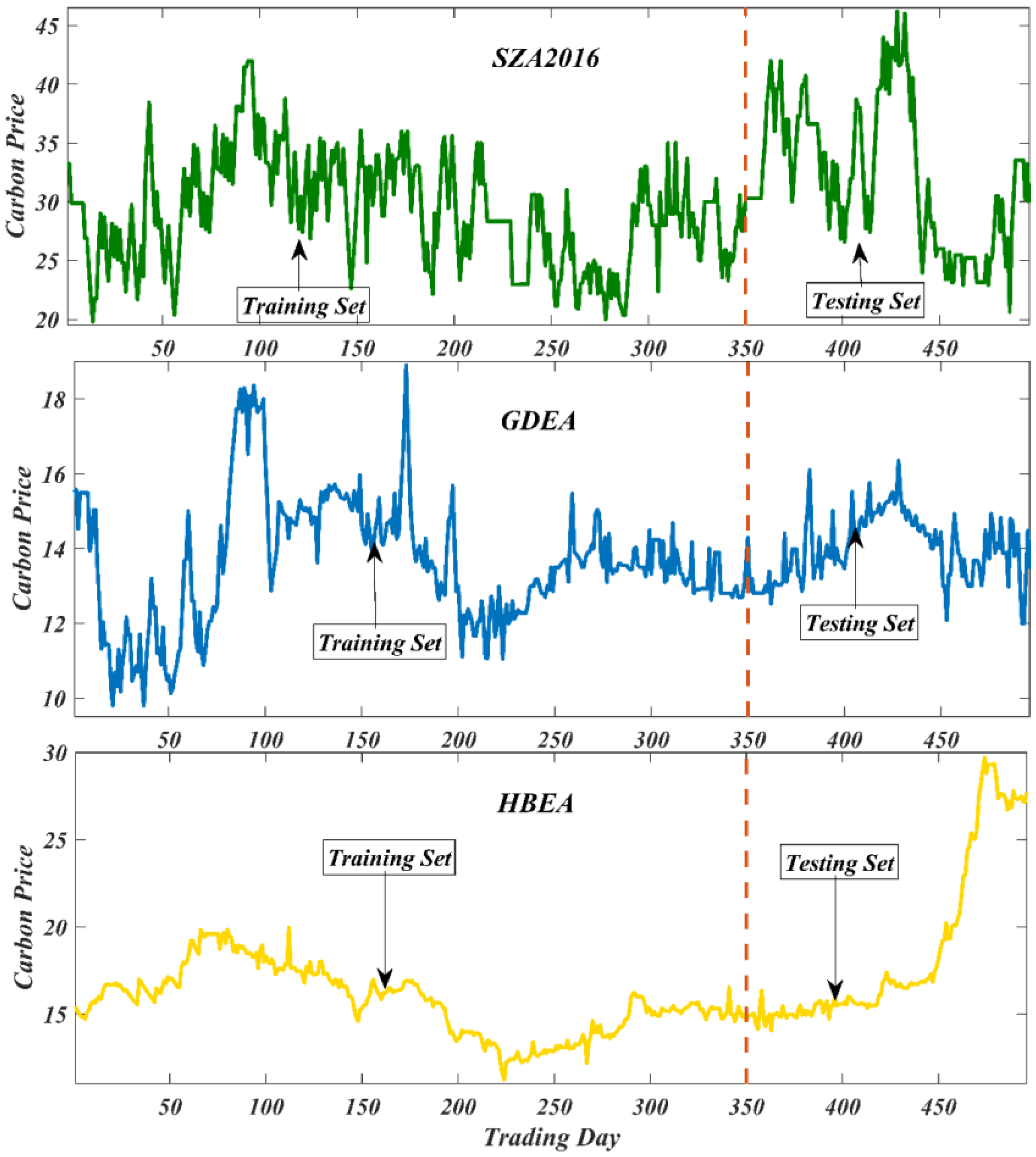
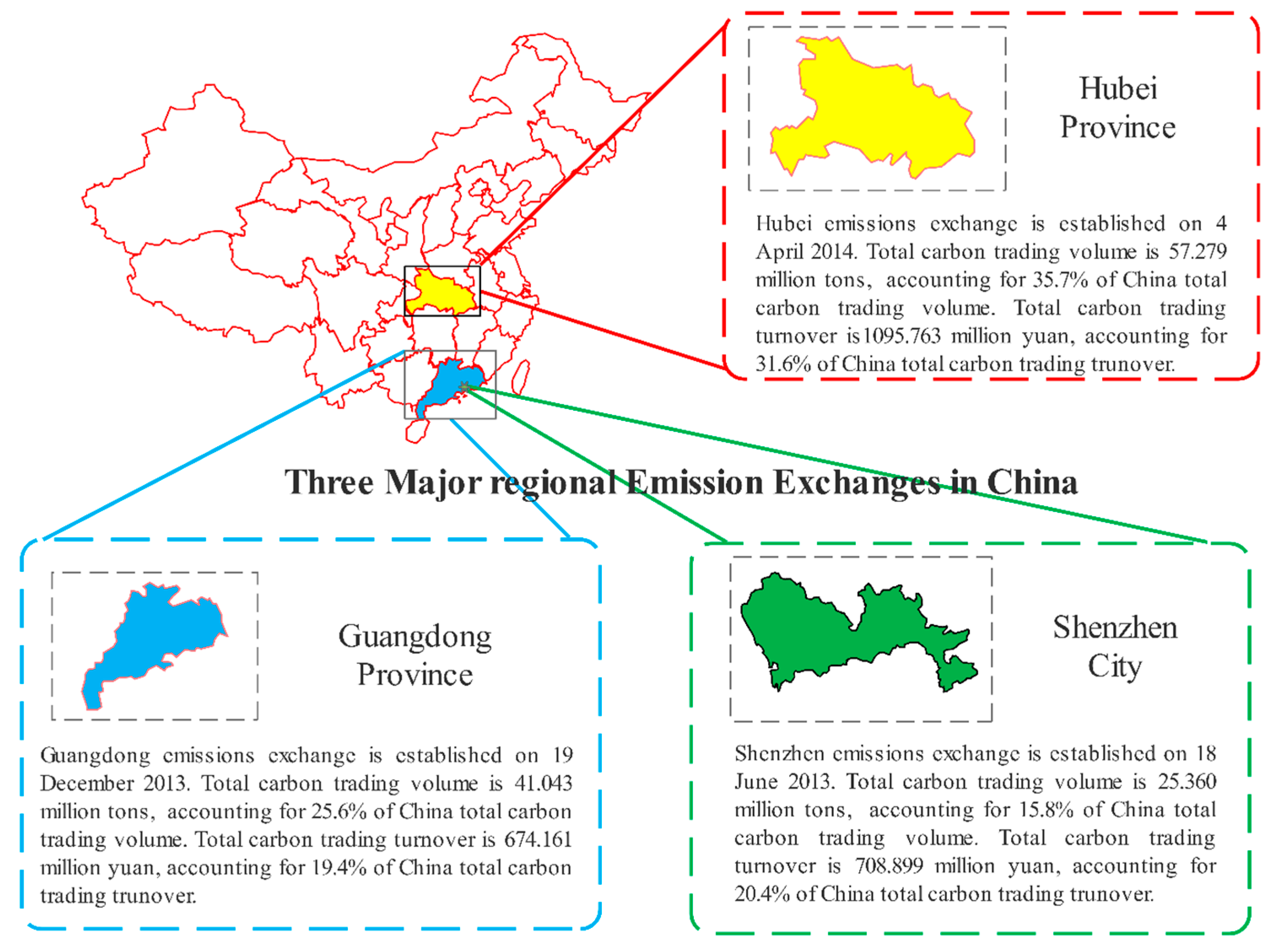
3.1. Data Descriptions

Considering the data availability, continuity, and comparability, three carbon price series used in this paper: SZA2016 from Shenzhen emission exchange, GDEA from Guangzhou emissions exchange, and HBEA from Hubei emissions exchange. SZA2016, HBEA, and GDEA are three actively traded assets that help to provide continuous carbon prices for study. The samples are obtained from 1 September 2016 to 11 September 2018, excluding non-trading days, with 496 data points included per series [47]. Three carbon prices are plotted in Figure 4. The basic information of the three regional emission exchanges is shown in Figure 5. The total carbon trading volume of these emission exchanges account for 77.1% of China’s total carbon trading volume, and the total carbon trading turnover of these emissions exchanges account for 71.4% of China’s total carbon trading turnover. These emission exchanges are three major pilot regional carbon emission exchanges in China.

The statistical descriptions of the three carbon price series are shown in

Table 1. Data descriptions for the three carbon price series.

Asset	Data	Count	Mean	Std	Min	25%	50%	75%	Max	Skew	Kurt
	All samples	496	29.99	5.23	19.80	25.91	29.81	33.23	46.20	0.47	−0.14
SZA2016	Training	350	29.09	4.53	19.80	25.60	28.99	32.39	42.00	0.22	−0.31
	Testing	146	32.13	6.12	20.64	26.87	30.63	36.83	46.20	0.28	−0.92
	All samples	496	13.74	1.52	9.80	12.87	13.70	14.69	18.90	0.27	0.86
GDEA	Training	350	13.62	1.71	9.80	12.59	13.50	14.70	18.90	0.42	0.43
	Testing	146	14.01	0.86	12.00	13.29	13.99	14.63	16.35	0.09	−0.51
	All samples	496	16.62	3.39	11.26	14.93	15.85	17.29	29.70	2.05	4.64
HBEA	Training	350	15.73	1.91	11.26	14.31	15.70	16.91	19.97	0.09	−0.57
	Testing	146	18.76	4.90	14.07	15.46	16.54	20.40	29.70	1.14	−0.34

Notes: Count denotes the number of samples, std is short for standard deviation, min denotes the minimum, max denotes the maximum, skew is short for skewness, and kurt is short for kurtosis. SZA2016 is short for Shenzhen emission allowance 2016, GDEA is short for Guangdong emission allowance, and HBEA is short for Hubei emission allowance.

. The average carbon price and price volatility of SZA2016 are higher than those of the HBEA and GDEA, which is also evident in Figure 4.

3.2. Evaluation Criteria

To measure the forecasting performance, three criteria (the mean absolute percentage error (MAPE) as calculated in Equation (23), the mean absolute error (MAE) as calculated in Equation (24), and the root mean square error (RMSE) as calculated in Equation (25)) are used. The process of the evaluation criteria is detailed in

Table 2. The evaluation metrics of forecasting performance.

Metric	Definition	Equation
MAPE	the mean absolute percentage error	$MAPE=\frac{1}{n}{\displaystyle \sum _{t=1}^n\left|\frac{y_{actual}-{\widehat{y}}_{forecasted}}{y_{actual}}\right|}\times 100\%$ (1)
MAE	the mean absolute error	$MAE=\frac{1}{n}{\displaystyle \sum _{t=1}^n\left|y_{actual}-{\widehat{y}}_{forecasted}\right|}$ (2)
RMSE	the root mean of square error	$RMSE=\sqrt{\frac{1}{n}{\displaystyle \sum _{t=1}^n{\left|y_{actual}-{\widehat{y}}_{forecasted}\right|}^2}}$ (3)

where $y_{actual}$ is the actual value and ${\widehat{y}}_{forecasted}$ is the forecasted value, and $n$ is the number of forecasted points. The smaller the above three criteria are, the higher forecasting accuracy the model achieves.

.

3.3. Data Preprocessing

As shown in Figure 4 and Table 1, carbon price series are heavily random and highly volatile. To eliminate noise, VMD is applied to preprocess the raw carbon price series. After VMD, the raw carbon price series are decomposed into some IMFs. Furthermore, the IMFs are reconstructed to obtain the preprocessed data. VMD remains the major mode in the price series. The preprocessed carbon price series are smoother than the raw series which can significantly improve the effectiveness and accuracy of time series prediction [46].

3.4. Parameter Setting and Input Selection

The general expression for the input and output of the model can be described as follows:

$$\left[x_{t+1},x_{t+2},x_{t+3}\right]=model\left(x_t,x_{t-1},\dots ,x_{t-m}\right)$$

(26)

where the input lag is $m+1$, $x_t$ is the observation value at time $t$, $x_{t+1},x_{t+2},x_{t+3}$ are one-step, two-step, and three-step forecasted values, respectively. In the FMRVR, the radial basis function (RBF) kernel is chosen as the kernel function which is expressed in Equation (27), with kernel width (i.e., a free parameter) $\upsilon$:

$$K\left(x,x^{\prime }\right)=\exp \left(-\frac{\Vert x-x^{\prime }\Vert }{2\upsilon }\right)$$

(27)

The input lag and kernel width are two parameters that are optimized in the MOWOA. The parameters setting used to train the VMD-FMRVR-MOWOA is shown in

Table 3. Parameter setting used in the VMD-FMRVR-MOWOA to train the model.

Modules	Parameter	Value
VMD	Number of IMFs (Intrinsic Mode Functions )	6
	Omegas initialization	Uniformly distributed
	Tolerance of convergence criterion	10−7
FMRVR	Width of kernel function	Select within [0.1,5]
	Input lags	Select within [1,20]
	Kernel type	Gaussian kernel
	Maximum iteration number of EM (expectation-maximization) algorithm	1000
	Tolerance value to check convergence of EM algorithm	0.1
MOWOA	Number of search agents	10
	Maximum number of iterations	20
	Maximum number of archives	10
	The dimension of the problem	3

. The objective function used in MOWOA is $\left\{RMS{E}_1,RMS{E}_2,RMS{E}_3\right\}$, where the RMSE is achieved in one-step, two-step, and three-step ahead forecasting, respectively.

3.5. Compared Models

The proposed model is compared with the other five multi-output forecasting models: FMRVR-MOWOA (proposed in this paper), MOGP-MOWOA (multi-output Gaussian process regression optimized [48] by MOWOA, where the Gaussian process regression is also widely used in time series forecasting [49,50]), MOTP-MOWOA (multi-output student-t process regression [48] optimized by MOWOA), MSVR (multi-output support vector regression [51]), and BPNN (back propagation neural network [52,53]).

The parameter setting in FMRVR-MOWOA is similar to that in Table 3. The parameter settings (input lags, initial covariance, and scale in the kernel function) in MOTP-MOWOA and MOGP-MOWOA are optimized by the MOWOA. The parameters in MSVR, the $\epsilon$ loss function parameter and the error trade-off parameter are optimized by a grid optimization algorithm. BPNN is a 6-13-3 structure network, where the maximum number of iterations is 1000 and the training precision is 0.00004.

3.6. Results and Discussion

Table 4. The one-step, two-step, and three-step ahead forecasting performance comparisons of SZA2016 for different forecasting models.

Models	1-Step			2-Step			3-Step
	MAPE	MAE	RMSE	MAPE	MAE	RMSE	MAPE	MAE	RMSE
VMD-FMRVR-MOWOA	6.738%	2.164	2.655	8.278%	2.677	3.373	9.646%	3.122	4.009
FMRVR-MOWOA	7.538%	2.405	2.960	9.310%	3.001	3.757	11.057%	3.565	4.449
MOTP-MOWOA	8.715%	2.812	3.522	10.830%	3.484	4.309	12.081%	3.896	4.749
MOGP-MOWOA	9.215%	3.076	4.198	10.526%	3.495	4.574	11.448%	3.752	4.772
MSVR	8.237%	2.708	3.525	10.015%	3.269	4.283	11.484%	3.798	5.012
BPNN	7.724%	2.477	3.135	9.361%	3.018	3.932	10.457%	3.367	4.390

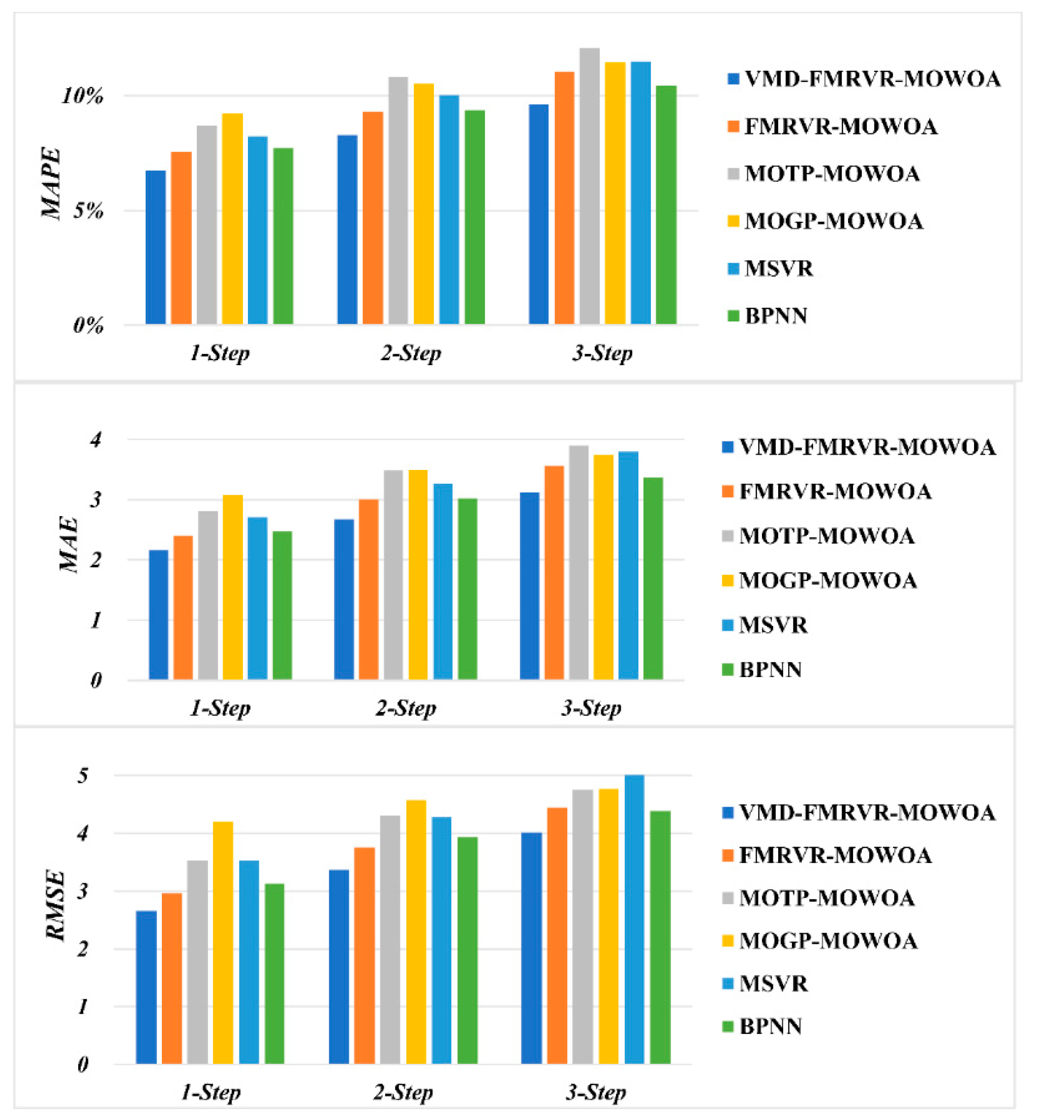
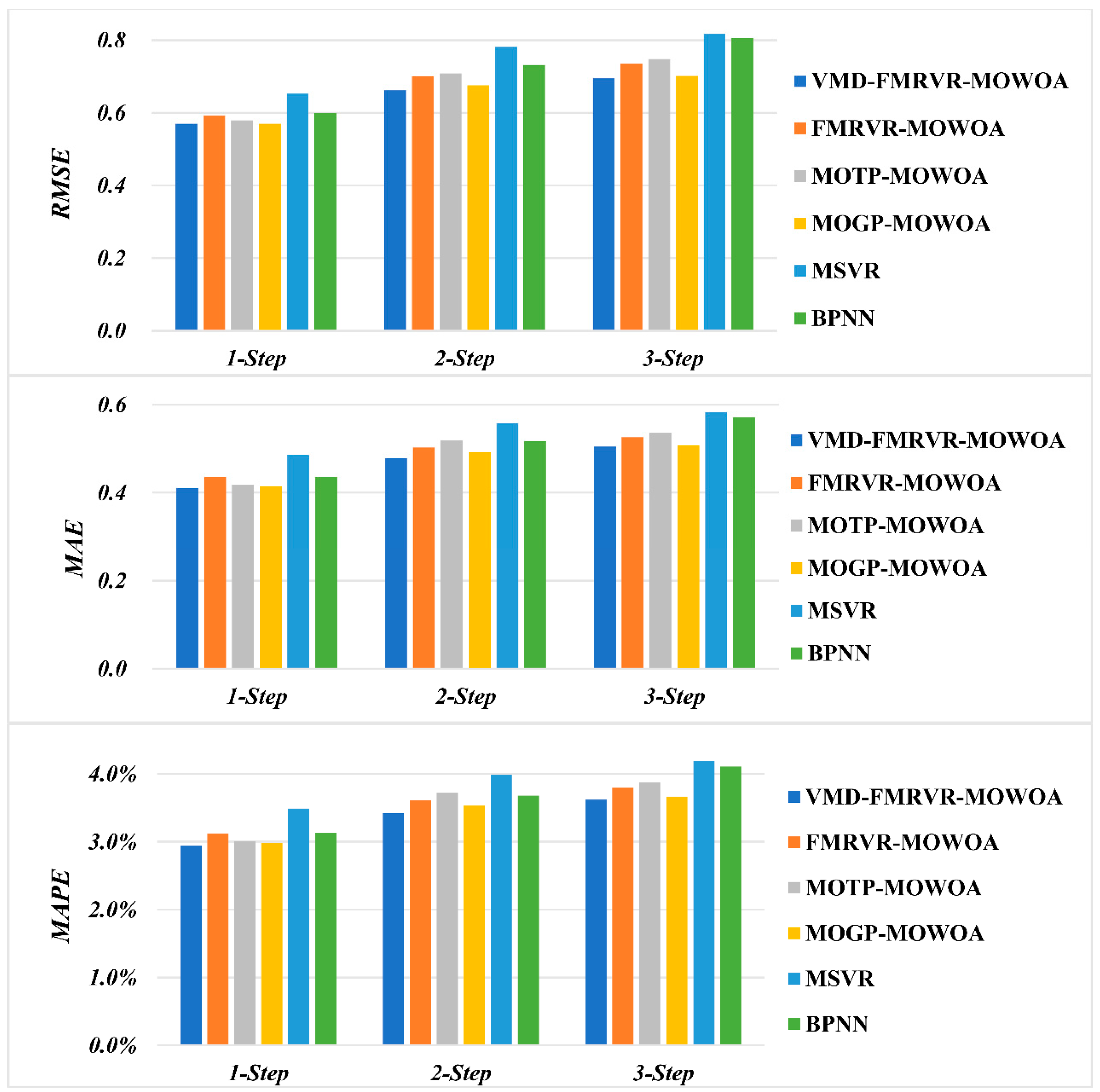
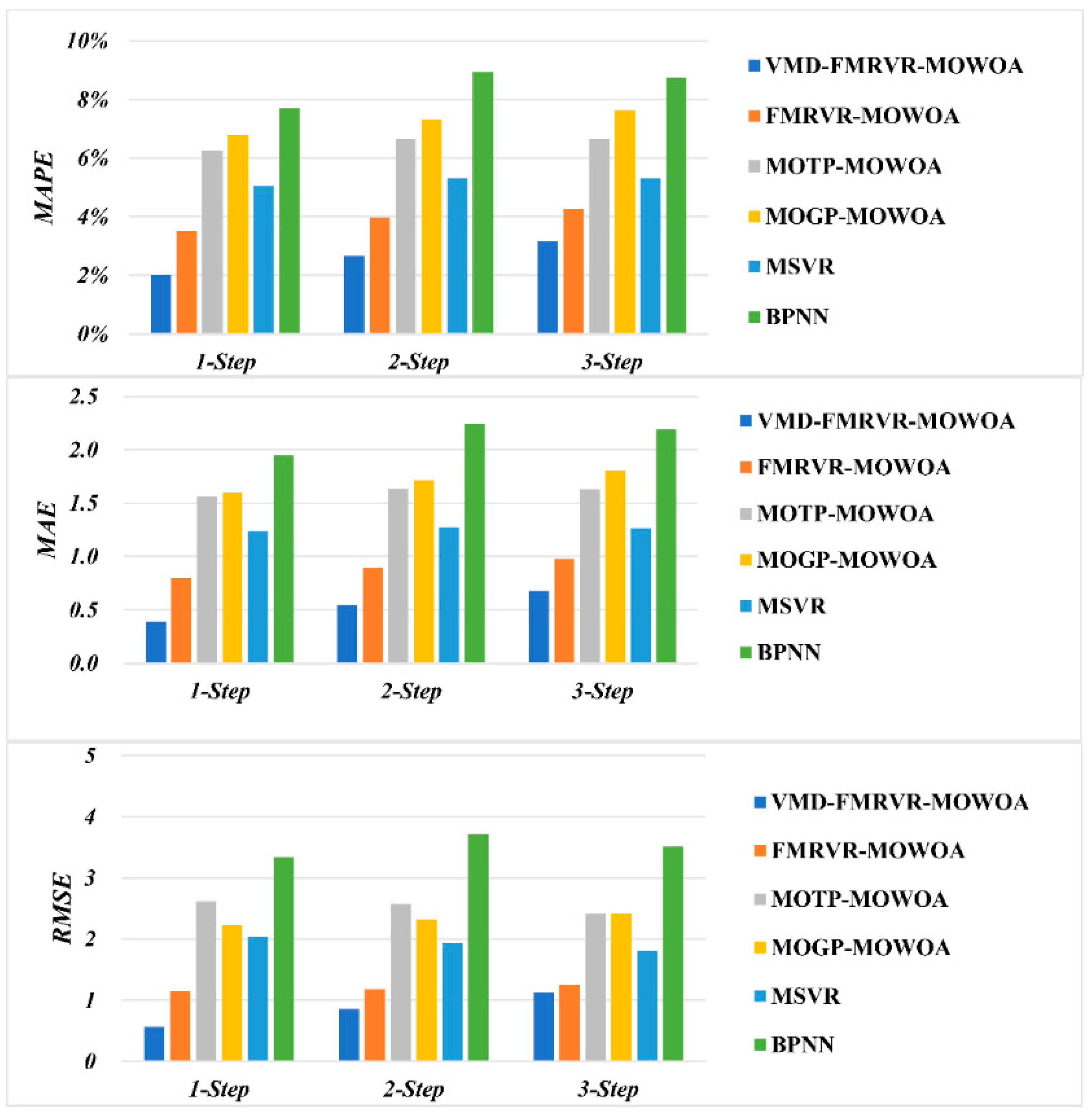
Notes: MOTP=multi-output student-t process regression, MOGP=multi-output Gaussian process regression, MSVR=multi-output support vector regression and BPNN=back propagation neural network.

presents the forecasting results of SZA2016 from the different models. For clarity, the values of MAPE, MAE, and RMSE are plotted in Figure 6. As shown in Table 4 and Figure 6, VMD-FMRVR-MOWOA outperforms the other five models in all three steps ahead forecasts. The results show the following:

(a)

The proposed model has the smallest MAPE, MAE, and RMSE in one-step, two-step, and three-step ahead forecasting performance. The MAPE values achieved by the proposed model are 6.738%, 8.278%, and 9.646% in one-step, two-step, and three-step ahead forecasting, respectively. The smallest MAPE values from the remaining five models are 7.538%, 9.310%, and 10.457% in the one-step, two-step, and three-step ahead forecasts achieved by FMRVR-MOWOA, FMRVR-MOWOA, and BPNN, respectively. The MAE values achieved using the proposed model are 2.164, 2.677, and 3.122 in one-step, two-step, and three-step ahead forecasting, respectively. The smallest MAE values from the remaining five models are 2.405, 3.001, and 3.367 in one-step, two-step, and three-step ahead forecasting achieved by the FMRVR-MOWOA, FMRVR-MOWOA, and BPNN, respectively. The RMSE values achieved by the proposed model are 2.655, 3.373, and 4.009 in one-step, two-step, and three-step ahead forecasting, respectively. The smallest RMSE values from the remaining five models are 2.960, 3.757, and 4.390 in one-step, two-step, and three-step ahead forecasting achieved by FMRVR-MOWOA, FMRVR-MOWOA, and BPNN, respectively. The MAPE, MAE, and RMSE obtained by the proposed model are smaller than the smallest MAPE, MAE, and RMSE values achieved by the other five models, respectively. These results show that the proposed method has a high accuracy in forecasting SZA2016 price series.

(b)

The proposed model outperforms the FMRVR-MOWOA in all of the one-step, two-step, and three-step ahead forecasting, which can be mainly attributed to the fact that VMD denoises the carbon price series. This shows that the VMD algorithm helps to improve the forecasting performance in carbon price series.

(c)

The proposed model outperforms the MOTP-MOWOA and MOGP-MOWOA in one-step, two-step, and three-step ahead forecasting. These results show that the VMD-FMRVR has a stronger performance in SZA2016 price forecasting than the MOTP and MOGP.

(d)

Forecasting accuracy decreases as the forecasting step size increases. All MAPE, MAE, and RMSE values increase by the increase in one-step, two-step, and three-step ahead forecasting for all six models. These results indicate that the difficulty in forecasting increases with the forecasting step.

The forecasting performances for GDEA and HBEA are presented in

Table 5. The one-step, two-step, and three-step ahead forecasting performance comparisons of GDEA with different forecasting models.

MODELS	1-Step			2-Step			3-Step
	MAPE	MAE	RMSE	MAPE	MAE	RMSE	MAPE	MAE	RMSE
VMD-FMRVR-MOWOA	2.944%	0.411	0.570	3.422%	0.478	0.662	3.620%	0.504	0.694
FMRVR-MOWOA	3.117%	0.435	0.593	3.607%	0.502	0.700	3.796%	0.526	0.735
MOTP-MOWOA	3.005%	0.419	0.579	3.717%	0.518	0.709	3.873%	0.536	0.748
MOGP-MOWOA	2.981%	0.414	0.570	3.537%	0.492	0.676	3.666%	0.508	0.701
MSVR	3.489%	0.486	0.654	3.994%	0.558	0.782	4.183%	0.583	0.819
BPNN	3.128%	0.436	0.599	3.679%	0.518	0.731	4.107%	0.571	0.805

and

Table 6. The one-step, two-step, and three-step ahead forecasting performance comparisons of HBEA for different forecasting models.

MODELS		1-Step			2-Step			3-Step
	MAPE	MAE	RMSE	MAPE	MAE	RMSE	MAPE	MAE	RMSE
VMD-FMRVR-MOWOA	2.018%	0.390	0.565	2.668%	0.549	0.856	3.149%	0.677	1.125
FMRVR-MOWOA	3.506%	0.799	1.143	3.969%	0.899	1.186	4.267%	0.975	1.250
MOTP-MOWOA	6.271%	1.561	2.615	6.666%	1.632	2.577	6.665%	1.630	2.420
MOGP-MOWOA	6.792%	1.596	2.228	7.302%	1.711	2.322	7.645%	1.804	2.419
MSVR	5.046%	1.236	2.038	5.303%	1.273	1.934	5.299%	1.268	1.807
BPNN	7.701%	1.948	3.343	8.928%	2.248	3.719	8.747%	2.194	3.515

, respectively. For clarity, the MAPE, MAE, and RMSE values are presented in Figure 7 and Figure 8. Similar to the results for SZA2016 forecasting shown in Table 4, the proposed model outperforms the other five models in multi-step-ahead forecasting given its stability in GDEA and HBEA price series forecasting.

As shown in Table 5 and Figure 7, there is a small difference among the six models in the forecasting performance of the GDEA price series. For one-step, two-step, and three-step ahead forecasting, the smallest MAPE values are 2.944%, 3.422%, and 3.620%, respectively; the smallest MAE values are 0.411, 0.478, and 0.504, respectively; and the lowest RMSE are 0.570, 0.662, and 0.694, respectively. These smallest MAPE, MAE, and RMSE values are all achieved by the proposed model, which implies that the proposed model outperforms the other five models in the multi-step-ahead forecasting of GDEA price series.

As shown in Table 6 and Figure 8, the forecasting performance for HBEA price series with the six models is described. For one-step, two-step, and three-step ahead forecasting, the MAPE values achieved by the proposed model are 2.018%, 2.668%, and 3.149%; the MAE values achieved by the proposed model are 0.390, 0.549, and 0.677; and the RMSE values achieved by the proposed model are 0.565, 0.85, and 1.125, respectively. All of these criteria rank first in the six models. These results imply that the proposed model outperforms the other five models in the multi-step-ahead forecasting of the HBEA price series.

3.7. Improvement of the Proposed Hybrid Model

Three criteria are applied to measure the improvement ratio of the proposed model compared to the other five models in terms of forecasting performance, which helps make an intuitionistic analysis. The criteria are defined in

Table 7. Improvement ratio of MAPE, MAE, and RMSE.

Metric	Definition	Equation
$P_{MAPE}$	improvement ratio of MAPE	$P_{MAPE}=\left|\frac{MAP{E}_{compared}-MAP{E}_{proposed}}{MAP{E}_{compared}}\right|\times 100\%$ (4)
$P_{MAE}$	improvement ratio of MAE	$P_{MAE}=\left|\frac{MA{E}_{compared}-MA{E}_{proposed}}{MA{E}_{compared}}\right|\times 100\%$ (5)
$P_{RMSE}$	improvement ratio of RMSE	$P_{RMSE}=\left|\frac{RMS{E}_{compared}-RMS{E}_{proposed}}{RMS{E}_{compared}}\right|\times 100\%$ (6)

where $MAP{E}_{proposed}$, $MA{E}_{proposed}$, and $RMS{E}_{proposed}$ are the forecasting performance achieved by the proposed model. $MAP{E}_{compared}$, $MA{E}_{compared}$, and $RMS{E}_{compared}$ are the forecasting performance achieved by the other model. $P_{MAPE}$, $P_{MAE}$, and $P_{RMSE}$ are the improvement ratio in MAPE, MAE, and RMSE, respectively.

.

The improvement ratio of the proposed model compared to the other five models is calculated for the three forecasted carbon price series. The improvements in one-step, two-step, and three-step ahead forecasting with respect to the MAPE, MAE, and RMSE are shown in

Table 8. Improvement ratio of MAPE with the proposed hybrid model compared to other models in one-step, two-step, and three-step ahead forecasting.

MODELS		SZA2016			GDEA			HBEA
	1-Step	2-Step	3-Step	1-Step	2-Step	3-Step	1-Step	2-Step	3-Step
FMRVR-MOWOA	10.614%	11.082%	12.763%	5.551%	5.146%	4.643%	42.440%	32.777%	26.191%
MOTP-MOWOA	22.689%	23.566%	20.153%	2.030%	7.950%	6.533%	67.824%	59.977%	52.748%
MOGP-MOWOA	26.886%	21.359%	15.744%	1.221%	3.244%	1.252%	70.292%	63.464%	58.804%
MSVR	18.201%	17.340%	16.007%	15.608%	14.321%	13.457%	60.010%	49.690%	40.573%
BPNN	12.765%	11.571%	7.755%	5.875%	6.991%	11.854%	73.797%	70.117%	63.997%

,

Table 9. Improvement ratio of MAE with the proposed hybrid model compared to other models in one-step, two-step, and three-step ahead forecasting.

MODELS		SZA2016			GDEA			HBEA
	1-Step	2-Step	3-Step	1-Step	2-Step	3-Step	1-Step	2-Step	3-Step
FMRVR-MOWOA	10.035%	10.821%	12.415%	5.545%	4.811%	4.111%	51.278%	38.932%	30.576%
MOTP-MOWOA	23.049%	23.172%	19.869%	1.917%	7.665%	5.957%	75.050%	66.372%	58.452%
MOGP-MOWOA	29.656%	23.421%	16.795%	0.840%	2.790%	0.648%	75.602%	67.926%	62.478%
MSVR	20.103%	18.127%	17.798%	15.478%	14.359%	13.419%	68.478%	56.888%	46.598%
BPNN	12.629%	11.312%	7.277%	5.795%	7.598%	11.597%	80.006%	75.583%	69.135%

and

Table 10. Improvement ratio of RMSE with the proposed hybrid model compared to other models in one-step, two-step, and three-step ahead forecasting.

MODELS		SZA2016			GDEA			HBEA
	1-Step	2-Step	3-Step	1-Step	2-Step	3-Step	1-Step	2-Step	3-Step
FMRVR-MOWOA	10.301%	10.230%	9.874%	3.984%	5.417%	5.559%	50.561%	27.837%	9.989%
MOTP-MOWOA	24.634%	21.730%	15.574%	1.670%	6.596%	7.167%	78.384%	66.798%	53.507%
MOGP-MOWOA	36.767%	26.261%	15.973%	0.052%	2.041%	0.972%	74.634%	63.151%	53.480%
MSVR	24.696%	21.241%	20.007%	12.838%	15.338%	15.198%	72.270%	55.757%	37.723%
BPNN	15.328%	14.215%	8.662%	4.870%	9.491%	13.768%	83.095%	76.993%	67.986%

, respectively. Some discussions are as follows:

(a)

For the improvement ratio in the MAPE shown in Table 8, the largest improvement ratios for one-step, two-step, and three-step ahead forecasting of SZA2016 are 26.886%, 23.566%, and 20.153%, and the smallest improvement ratios are 10.614%, 11.082%, and 7.755%, respectively. These results show that the proposed model outperforms the other five models and shows a steady performance in forecasting of SZA2016. Similar results are also shown in the MAPE improvement ratio for GDEA and HBEA.

(b)

For the improvement ratio of the MAE and RMSE, consistent with that of MAPE shown in Table 8, the results presented in Table 9 and Table 10 suggest that the proposed model outperforms the other five models in all SZA2016, GDEA, and HBEA forecasts.

To check the overall performance of the proposed model, the average improvement ratios of the proposed model over the three carbon price series forecasting are presented in

Table 11. Average improvement ratio of the proposed hybrid model with respect to MAPE, MAE, and RMSE for the three carbon prices series in China’s emissions exchanges.

		MAPE			MAE			RMSE
MODELS	1-Step	2-Step	3-Step	1-Step	2-Step	3-Step	1-Step	2-Step	3-Step
FMRVR-MOWOA	19.535%	16.335%	14.532%	22.286%	18.188%	15.701%	21.615%	14.495%	8.474%
MOTP-MOWOA	30.848%	30.498%	26.478%	33.339%	32.403%	28.093%	34.896%	31.708%	25.416%
MOGP-MOWOA	32.799%	29.356%	25.267%	35.366%	31.379%	26.640%	37.151%	30.484%	23.475%
MSVR	31.273%	27.117%	23.346%	34.686%	29.791%	25.938%	36.601%	30.779%	24.309%
BPNN	30.813%	29.559%	27.869%	32.810%	31.498%	29.336%	34.431%	33.566%	30.139%

.

As shown in Table 11, the smallest average improvements in the MAPE for one-step, two-step, and three-step ahead forecasting are 19.535%, 16.335%, and 14.532%, and the largest average improvements in the MAPE are 32.799%, 30.498%, and 27.869%, respectively. These results indicate that the proposed model outperforms the other five models in terms of MAPE performance.

Similarly, the smallest average improvements in the MAE for one-step, two-step, and three-step ahead forecasting are 22.286%, 18.188%, and 15.701%, and the largest average improvement in the MAE are 35.366%, 32.403%, and 29.336%, respectively. These results show that the proposed model achieves better performance in the MAE than the other five models.

The smallest average improvements in the RMSE for one-step, two-step, and three-step ahead forecasting are 21.615%, 14.495%, and 8.474%, and the largest average improvements in RMSE are 36.601%, 33.566%, and 30.139%, respectively. These results suggest that the proposed model exceeds the other five models with regards to the RMSE performance.

The above results show that the proposed model achieved the best forecasting performance among the six models with respect to the three performance criteria. The proposed model performs steadily in the multi-step-ahead forecasting of the three carbon price series.

4. Conclusions

The accurate and stable forecasting of carbon prices is important to promote the development of carbon markets and vital to reduce carbon emissions in China. However, improving forecasting accuracy is hard work due to the non-stationary characteristics of carbon prices, especially for multi-step-ahead forecasting. In this paper, we propose a hybrid multi-step-ahead forecasting model, VMD-FMRVR-MOWOA, for carbon price series. The proposed hybrid forecasting model is applied to three carbon price series from three major pilot regional carbon emission exchanges in China: SZA2016 from Shenzhen emission exchange, GDEA from Guangzhou emissions exchange, and HBEA from Hubei emissions exchange. The sample period of the three carbon price series is from 1 September 2016 to 11 September 2018. Compared with the other five multi-output models (FMRVR-MOWOA, MOTP-MOWOA, MOGP-MOWOA, MSVR, and BPNN), the proposed VMD-FMRVR-MOWOA model obtained the smallest MAPE, MAE, and RMSE in all of the one-step, two-step, and three-step ahead forecasting of the three carbon prices from the major regional emission exchange in China. The smallest average improvement ratio in MAPE, MSE, and RMSE of the proposed hybrid model compared with the other five models are 14.532%, 15.701%, and 8.474%, respectively. These results show that the proposed VMD-FMRVR-MOWOA model outperforms the other five multi-output models in terms of forecasting accuracy and stability, and it can be a potential and effective technique for multi-step-ahead carbon price forecasting in China’s major regional emission exchanges. The proposed model can help governors to deeply understand the characteristics of the carbon price in the three major regional emission exchanges in order to make a more reasonable carbon pricing mechanism, help companies make reasonable production arrangement to reduce cost and help market investors to control price risk. As a newly developed hybrid model, in our future work, we will test the forecasting performance of the proposed method in other forecasting fields, such as crude oil price and stock index.

References

1. Zhu, B.; Ye, S.; Wang, P.; He, K.; Zhang, T.; Wei, Y.-M. A novel multiscale nonlinear ensemble leaning paradigm for carbon price forecasting. Energy Econo. 2018, 70, 143–157. [Google Scholar] [CrossRef]
2. Ju, Y.; Fujikawa, K. Modeling the cost transmission mechanism of the emission trading scheme in China. Appl. Energy 2019, 236, 172–182. [Google Scholar] [CrossRef]
3. Zhu, B.; Han, D.; Wang, P.; Wu, Z.; Zhang, T.; Wei, Y.-M. Forecasting carbon price using empirical mode decomposition and evolutionary least squares support vector regression. Appl. Energy 2017, 191, 521–530. [Google Scholar] [CrossRef]
4. Zhang, Y.; Zhang, S. The impacts of GDP, trade structure, exchange rate and FDI inflows on China’s carbon emissions. Energy Policy 2018, 120, 347–353. [Google Scholar] [CrossRef]
5. International Energy Agency. CO2 Emissions from Fuel Combustion Highlights; International Energy Agency: Paris, France, 2017; Available online: http://t.cn/REVfVt7 (accessed on 20 December 2018).
6. Janssens-Maenhout, G.; Crippa, M.; Guizzardi, D.; Muntean, M.; Schaaf, E.; Olivier, J.G.J.; Peters, J.A.H.W.; Schure, K.M. Fossil CO2 and GHG emissions of all world countries. Publ. Off. Eur. Union 2017. [Google Scholar] [CrossRef]
7. Zhou, K.; Li, Y. An Empirical Analysis of Carbon Emission Price in China. Energy Procedia 2018, 152, 823–828. [Google Scholar] [CrossRef]
8. Zhu, B.; Shi, X.; Chevallier, J.; Wang, P.; Wei, Y.-M. An Adaptive Multiscale Ensemble Learning Paradigm for Nonstationary and Nonlinear Energy Price Time Series Forecasting. J. Forecast. 2016, 35, 633–651. [Google Scholar] [CrossRef]
9. Zhang, Y.-J.; Wei, Y.-M. An overview of current research on EU ETS: Evidence from its operating mechanism and economic effect. Appl. Energy 2010, 87, 1804–1814. [Google Scholar] [CrossRef]
10. Guðbrandsdóttir, H.N.; Haraldsson, H.Ó. Predicting the Price of EU ETS Carbon Credits. Syst. Eng. Procedia 2011, 1, 481–489. [Google Scholar] [CrossRef] [Green Version]
11. Paolella, M.S.; Taschini, L. An econometric analysis of emission allowance prices. J. Bank. Financ. 2008, 32, 2022–2032. [Google Scholar] [CrossRef] [Green Version]
12. Chevallier, J.; Sévi, B. On the realized volatility of the ECX CO2 emissions 2008 futures contract: Distribution, dynamics and forecasting. Ann. Financ. 2011, 7, 1–29. [Google Scholar] [CrossRef]
13. Zhu, Z.B.; Ming, W.Y. Carbon price prediction based on integration of GMDH, particle swarm optimization and least squares support vector machines. Syst. Eng.-Theory Pract. 2011, 31, 2264–2271. [Google Scholar]
14. Fan, X.; Li, S.; Tian, L. Chaotic characteristic identification for carbon price and an multi-layer perceptron network prediction model. Expert Syst. Appl. 2015, 42, 3945–3952. [Google Scholar] [CrossRef]
15. Wang, J.; Wang, Y.; Li, Y. A Novel Hybrid Strategy Using Three-Phase Feature Extraction and a Weighted Regularized Extreme Learning Machine for Multi-Step Ahead Wind Speed Prediction. Energies 2018, 11, 321. [Google Scholar] [CrossRef]
16. Wang, R.; Li, J.; Wang, J.; Gao, C. Research and Application of a Hybrid Wind Energy Forecasting System Based on Data Processing and an Optimized Extreme Learning Machine. Energies 2018, 11, 1712. [Google Scholar] [CrossRef]
17. Dong, Y.; Wang, J.; Wang, C.; Guo, Z. Research and Application of Hybrid Forecasting Model Based on an Optimal Feature Selection System—A Case Study on Electrical Load Forecasting. Energies 2017, 10, 490. [Google Scholar] [CrossRef]
18. Dong, Y.; Ma, X.; Ma, C.; Wang, J. Research and Application of a Hybrid Forecasting Model Based on Data Decomposition for Electrical Load Forecasting. Energies 2016, 9, 1050. [Google Scholar] [CrossRef]
19. Sun, G.; Chen, T.; Wei, Z.; Sun, Y.; Zang, H.; Chen, S. A Carbon Price Forecasting Model Based on Variational Mode Decomposition and Spiking Neural Networks. Energies 2016, 9, 54. [Google Scholar] [CrossRef]
20. Zhou, J.; Yu, X.; Yuan, X. Predicting the Carbon Price Sequence in the Shenzhen Emissions Exchange Using a Multiscale Ensemble Forecasting Model Based on Ensemble Empirical Mode Decomposition. Energies 2018, 11, 1907. [Google Scholar] [CrossRef]
21. Zhu, B.; Wei, Y. Carbon price forecasting with a novel hybrid ARIMA and least squares support vector machines methodology. Omega 2013, 41, 517–524. [Google Scholar] [CrossRef]
22. Atsalakis, G.S. Using computational intelligence to forecast carbon prices. Appl. Soft Comput. 2016, 43, 107–116. [Google Scholar] [CrossRef]
23. Guo, Z.; Zhao, W.; Lu, H.; Wang, J. Multi-step forecasting for wind speed using a modified EMD-based artificial neural network model. Renew. Energy 2012, 37, 241–249. [Google Scholar] [CrossRef]
24. Wang, J.; Yang, W.; Du, P.; Li, Y. Research and application of a hybrid forecasting framework based on multi-objective optimization for electrical power system. Energy 2018, 148, 59–78. [Google Scholar] [CrossRef]
25. Wang, J.; Li, Y. Multi-step ahead wind speed prediction based on optimal feature extraction, long short term memory neural network and error correction strategy. Appl. Energy 2018, 230, 429–443. [Google Scholar] [CrossRef]
26. Upadhyay, A.; Pachori, R.B. Instantaneous voiced/non-voiced detection in speech signals based on variational mode decomposition. J. Frank. Inst. 2015, 352, 2679–2707. [Google Scholar] [CrossRef]
27. Huang, S.-C.; Wu, T.-K. Combining wavelet-based feature extractions with relevance vector machines for stock index forecasting. Expert Syst. 2008, 25, 133–149. [Google Scholar] [CrossRef]
28. Fei, S.-W.; He, Y. Wind speed prediction using the hybrid model of wavelet decomposition and artificial bee colony algorithm-based relevance vector machine. Int. J. Electr. Power Energy Syst. 2015, 73, 625–631. [Google Scholar] [CrossRef]
29. Alamaniotis, M.; Bargiotas, D.; Bourbakis, N.G.; Tsoukalas, L.H. Genetic Optimal Regression of Relevance Vector Machines for Electricity Pricing Signal Forecasting in Smart Grids. IEEE Trans. Smart Grid 2015, 6, 2997–3005. [Google Scholar] [CrossRef]
30. Li, T.; Zhou, M.; Guo, C.; Luo, M.; Wu, J.; Pan, F.; Tao, Q.; He, T. Forecasting Crude Oil Price Using EEMD and RVM with Adaptive PSO-Based Kernels. Energies 2016, 9, 1014. [Google Scholar] [CrossRef]
31. Wang, Y.; Wang, H.; Srinivasan, D.; Hu, Q. Robust functional regression for wind speed forecasting based on Sparse Bayesian learning. Renew. Energy 2019, 132, 43–60. [Google Scholar] [CrossRef]
32. Wang, Y.; Xie, Z.; Hu, Q.; Xiong, S. Correlation aware multi-step ahead wind speed forecasting with heteroscedastic multi-kernel learning. Energy Convers. Manag. 2018, 163, 384–406. [Google Scholar] [CrossRef]
33. Thayananthan, A.; Navaratnam, R.; Stenger, B.; Torr, P.H.S.; Cipolla, R. Pose estimation and tracking using multivariate regression. Pattern Recognit. Lett. 2008, 29, 1302–1310. [Google Scholar] [CrossRef] [Green Version]
34. Ha, Y. Fast multi-output relevance vector regression. arXiv, 2017; arXiv:1704.05041. [Google Scholar]
35. Du, P.; Wang, J.; Yang, W.; Niu, T. Multi-step ahead forecasting in electrical power system using a hybrid forecasting system. Renew. Energy 2018, 122, 533–550. [Google Scholar] [CrossRef]
36. Heng, J.; Wang, J.; Xiao, L.; Lu, H. Research and application of a combined model based on frequent pattern growth algorithm and multi-objective optimization for solar radiation forecasting. Appl. Energy 2017, 208, 845–866. [Google Scholar] [CrossRef]
37. Wang, J.; Heng, J.; Xiao, L.; Wang, C. Research and application of a combined model based on multi-objective optimization for multi-step ahead wind speed forecasting. Energy 2017, 125, 591–613. [Google Scholar] [CrossRef]
38. Niu, T.; Wang, J.; Zhang, K.; Du, P. Multi-step-ahead wind speed forecasting based on optimal feature selection and a modified bat algorithm with the cognition strategy. Renew. Energy 2018, 118, 213–229. [Google Scholar] [CrossRef]
39. Wang, J.; Du, P.; Niu, T.; Yang, W. A novel hybrid system based on a new proposed algorithm—Multi-Objective Whale Optimization Algorithm for wind speed forecasting. Appl. Energy 2017, 208, 344–360. [Google Scholar] [CrossRef]
40. Dragomiretskiy, K.; Zosso, D. Variational Mode Decomposition. IEEE Trans. Signal Process. 2014, 62, 531–544. [Google Scholar] [CrossRef]
41. Tipping, M.E. Sparse bayesian learning and the relevance vector machine. J. Mach. Learn. Res. 2001, 1, 211–244. [Google Scholar] [CrossRef]
42. Thayananthan, A. Template-based Pose Estimation and Tracking of 3D Hand Motion. Ph.D. Thesis, University of Cambridge, Cambridge, UK, 2005. [Google Scholar]
43. Mirjalili, S.; Lewis, A. The Whale Optimization Algorithm. Adv. Eng. Softw. 2016, 95, 51–67. [Google Scholar] [CrossRef]
44. Edgeworth, F.Y. Mathematical Physics; P. Keagan: London, UK, 1881. [Google Scholar]
45. Pareto, V. Cours D’économie Politique; Librairie Droz: Genève, Suisse, 1964; Volume 1. [Google Scholar]
46. Niu, T.; Wang, J.; Lu, H.; Du, P. Uncertainty modeling for chaotic time series based on optimal multi-input multi-output architecture: Application to offshore wind speed. Energy Convers. Manag. 2018, 156, 597–617. [Google Scholar] [CrossRef]
47. Carbon Market Data. Available online: http://k.tanjiaoyi.com/ (accessed on 19 September 2018).
48. Chen, Z.; Wang, B.; Gorban, A.N. Multivariate Gaussian and Student$-t$ Process Regression for Multi-output Prediction. arXiv, 2017; arXiv:1703.04455. [Google Scholar]
49. Hu, J.; Wang, J.; Xiao, L. A hybrid approach based on the Gaussian process with t-observation model for short-term wind speed forecasts. Renew. Energy 2017, 114, 670–685. [Google Scholar] [CrossRef]
50. Hu, J.; Wang, J. Short-term wind speed prediction using empirical wavelet transform and Gaussian process regression. Energy 2015, 93, 1456–1466. [Google Scholar] [CrossRef]
51. Tuia, D.; Verrelst, J.; Alonso, L.; Perez-Cruz, F.; Camps-Valls, G. Multioutput Support Vector Regression for Remote Sensing Biophysical Parameter Estimation. IEEE Geosci. Remote Sens. Lett. 2011, 8, 804–808. [Google Scholar] [CrossRef]
52. Werbos, P. Beyond Regression: New Tools for Prediction and Analysis in the Behavioral Sciences. Ph.D. Dissertation, Harvard University, Cambridge, MA, USA, 1974. [Google Scholar]
53. Rumelhart, D.E.; Mcclelland, J.L. Parallel Distributed Processing: Explorations in the Microstructure of Cognition. Volume 1. Foundations; MIT Press: Cambridge, MA, USA, 1986; p. 564. [Google Scholar]
Figure 1. Flow chart of VMD-FMRVR-MOWOA. VMD = variational mode decomposition; FMRVR = fast multi-output relevance vector; MOWOA = multi-objective whale optimization algorithm.
Energies 12 00147 g001
Figure 2. The pseudo-code of the alternate direction method of multipliers (ADMM) algorithm for VMD.
Energies 12 00147 g002
Figure 3. The pseudo-code of the MOWOA algorithm.
Energies 12 00147 g003
Figure 4. Plots of the three studied carbon price series.
Energies 12 00147 g004
Figure 5. Basic information of the three studied carbon price series.
Energies 12 00147 g005
Figure 6. Model forecasting performance comparison for SZA2016.
Energies 12 00147 g006
Figure 7. Model forecasting performance comparison for GDEA.
Energies 12 00147 g007
Figure 8. Models forecasting performance comparison for HBEA.
Energies 12 00147 g008