Reinforcement Learning Based Energy Management Algorithm for Smart Energy Buildings


Abstract
:1. Introduction
- The energy management of a smart energy building is modeled using MDP to completely describe the state space, action space, transition probability, and reward function.
- We propose a Q-learning-based energy management algorithm that provides an optimal action of energy dispatch in the smart energy building. The proposed algorithm can minimize the total energy cost that takes into consideration the future cost by using only current system information, while most existing work for energy management of smart energy buildings focuses on the optimization based on 24 h ahead given or predicted future information.
- To reduce the convergence time of the Q-learning-based algorithm, we propose a simple Q-table initialization procedure, in which each value of Q-table is set to an instantaneous reward directly obtained by the reward function with an initial system condition.
- From the simulations using real-life data sets of building energy demand, PV generation, and vehicles parking records, it is verified that the proposed algorithm significantly reduces the energy cost of smart energy building under both Time-of-Use (ToU) and real-time energy pricing approaches, compared to a conventional optimization-based approach as well as the greedy and random approaches.
2. Related Work
2.1. Energy Management in Microgrid
2.2. Energy Management in V2G
2.3. Energy Management in Smart Energy Building
3. Energy Management System Model Using MDP
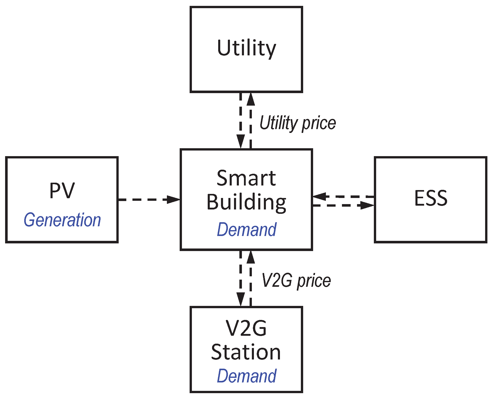
3.1. Overall System Structure
- “Utility” represents a company that supplies energy in real-time. It is assumed that the smart energy building is able to trade (buy and sell) energy with the utility company at any time at the prices determined by the utility company.
- “PV system” is a power supply system that converts sunlight into energy by means of photovoltaic panels. The energy generated by the PV system can be consumed to help meet the load demands of the smart energy building and V2G station.
- “V2G station” describes a system where EVs request charging (energy flow from the grid to EVs) or discharging (energy flow from EVs to the grid) services. It is assumed that the smart energy building trades energy based on the net demand of the V2G station, which can be either positive (if the number of EVs that require charging service is greater than the number of EVs that require discharging service) or negative (vice versa).
- “ESS” represents an energy storage system, capable of storing and releasing energy as needed in a flexible way. As a simple example, the smart energy building can utilize the ESS to decrease its operation cost by charging the ESS when energy prices are low and discharging the ESS when energy prices are high. We assume that the ESS considered in this paper consists of a combination of battery and super-capacitor. This hybrid ESS can take both the advantages of battery (high energy density and low cost per kWh) and super-capacitor (quick charging/discharging and extended lifetime) [23].
- “Building demand” represents the energy demand required by the smart energy building itself due to its internal energy consumption. The amount of energy demand of the building at each time step t is denoted by (kWh).
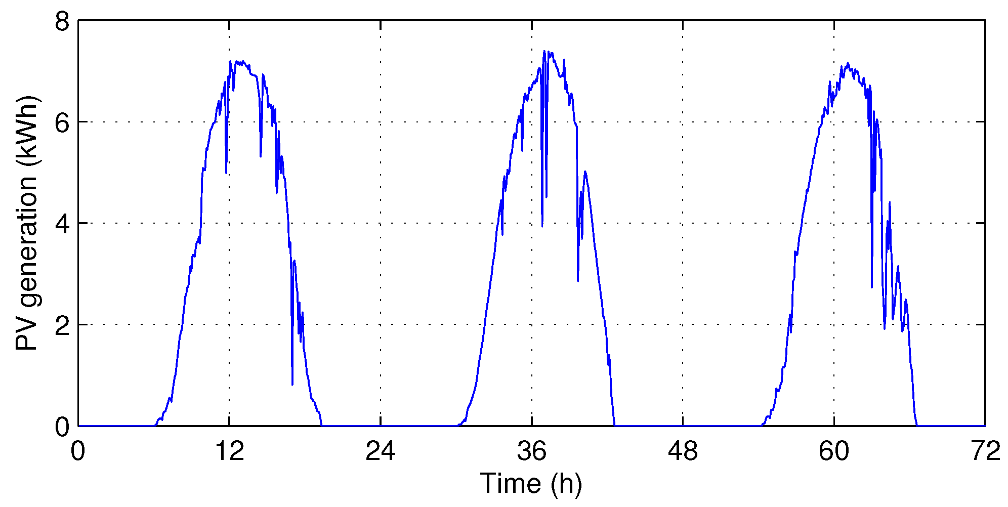
- “PV generation” represents the energy generated by the PV system, and is denoted by (kWh).
- “V2G demand” represents the energy demand of the V2G station, denoted by (kWh). Because the V2G station has bidirectional energy exchange capability with the building, there are two values of , a positive value when the V2G station draws energy from the building and a negative value when it supplies energy to the building.
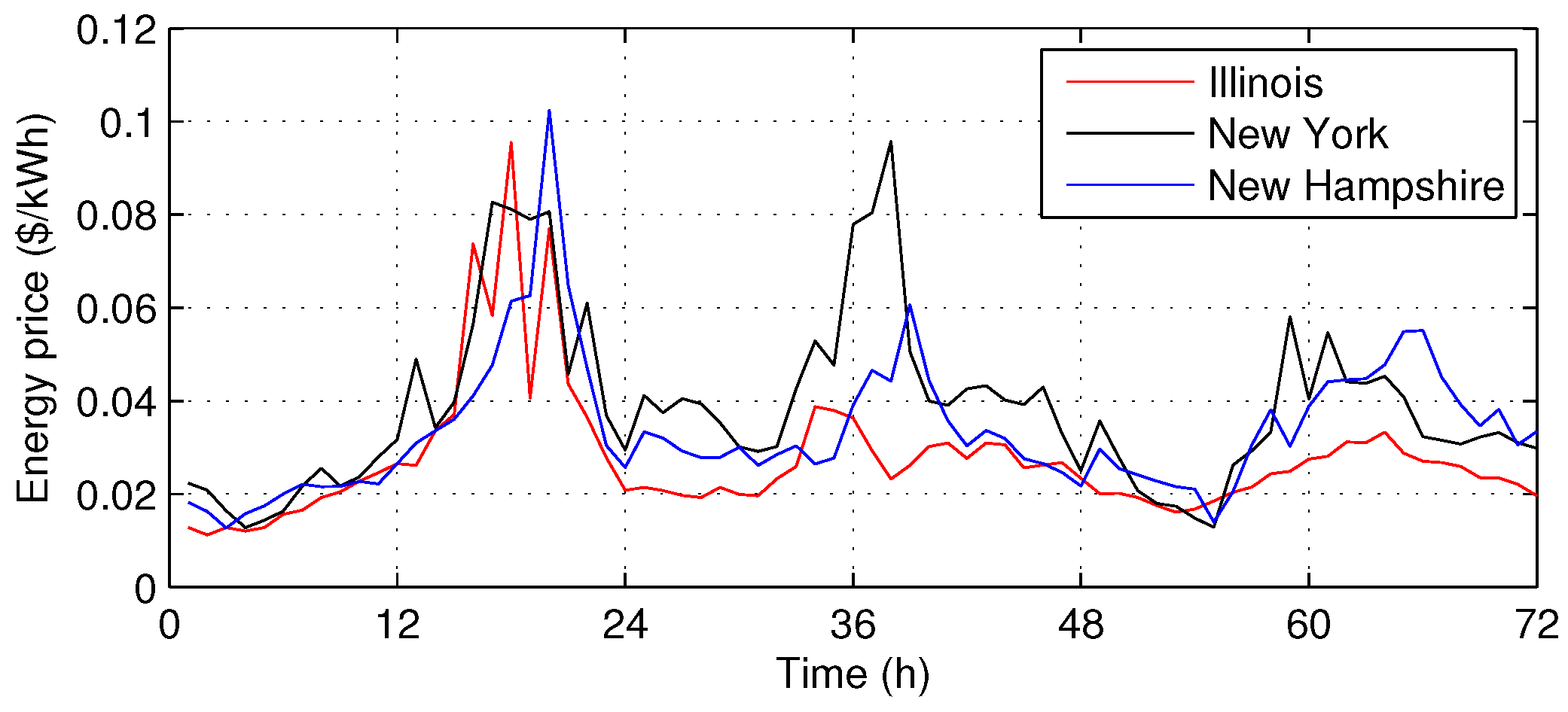
- “Utility price” represents the prices for energy transaction between the building and the utility company, and is denoted by ($/kWh).
- “V2G price” represents the energy prices for energy transaction when EVs are charged or discharged at V2G station, and is denoted by ($/kWh).
3.2. State Space
3.3. Action Space
3.4. Transition Probability
3.5. Reward Function
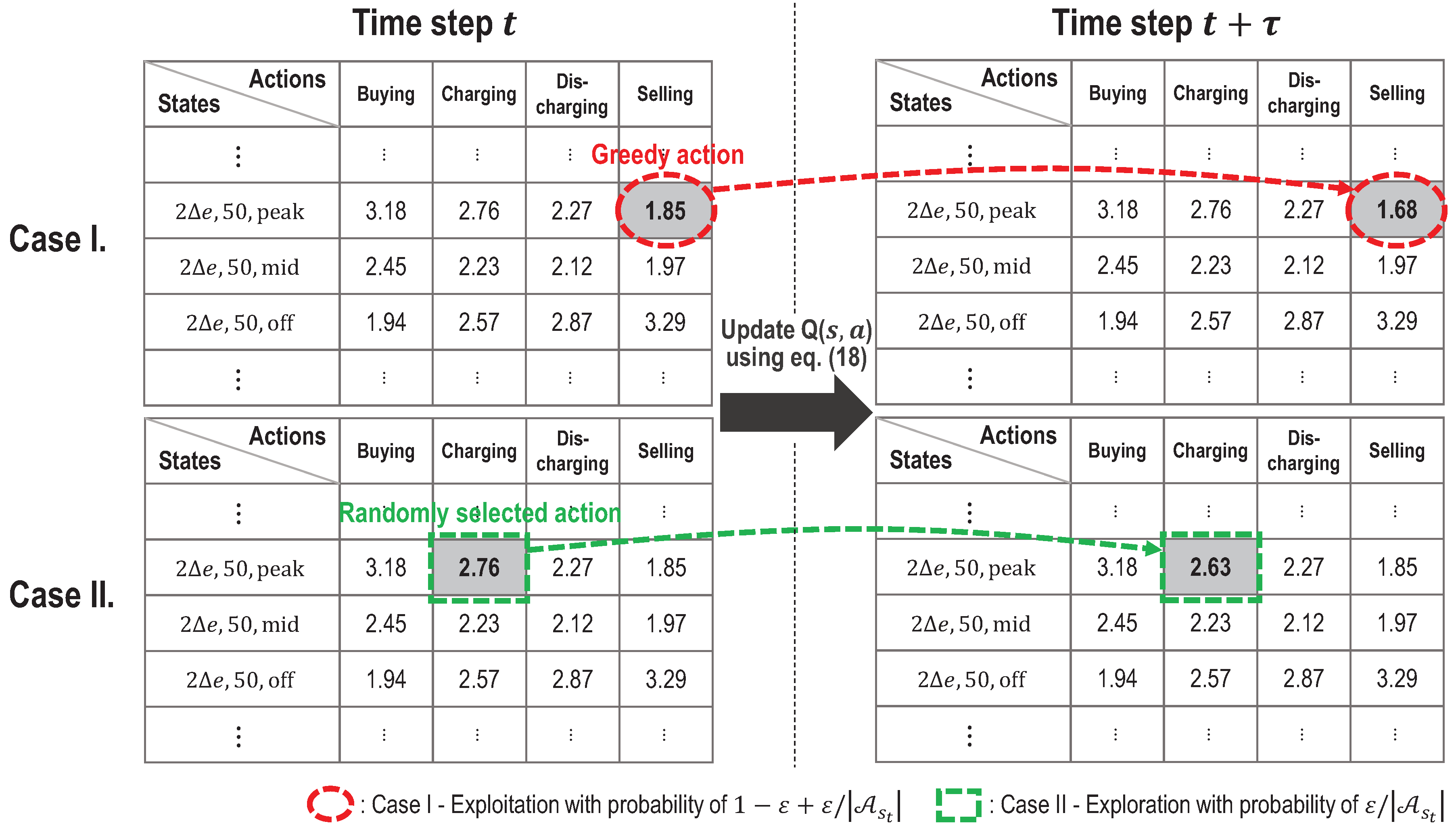
4. Energy Management Algorithm Using Q-Learning
| Algorithm 1 Energy management algorithm using Q-learning |
5. Performance Evaluation
5.1. Simulation Setting
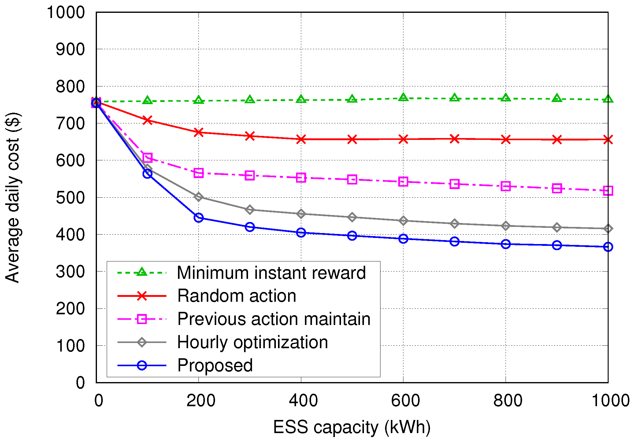
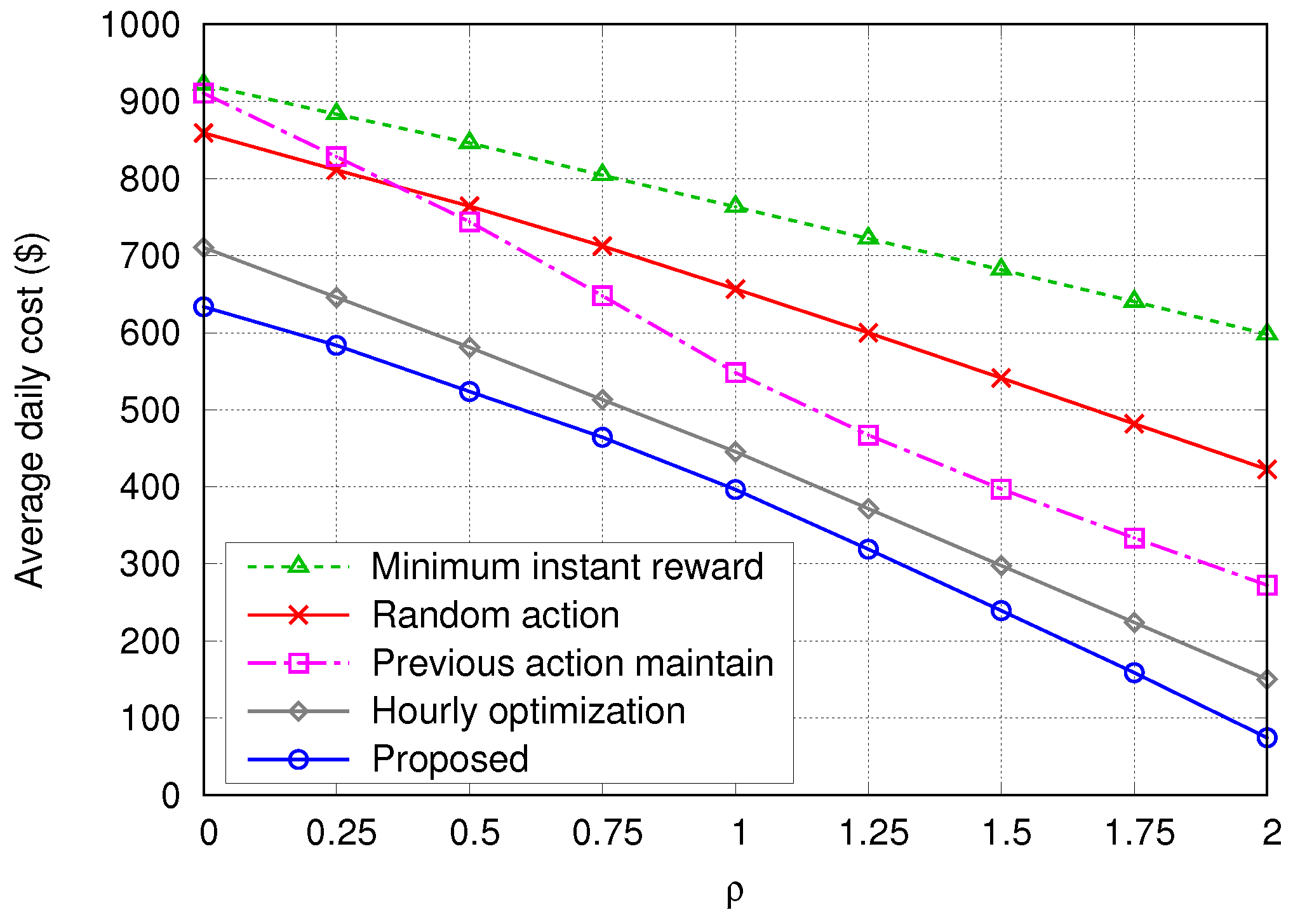
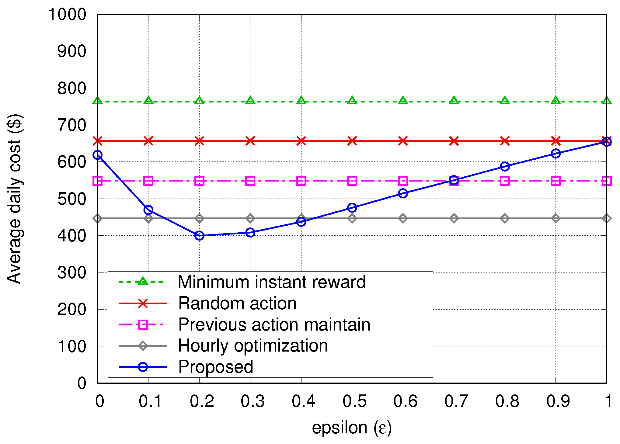
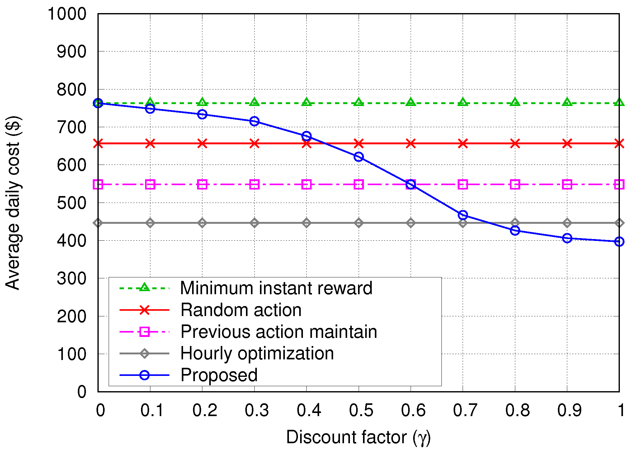
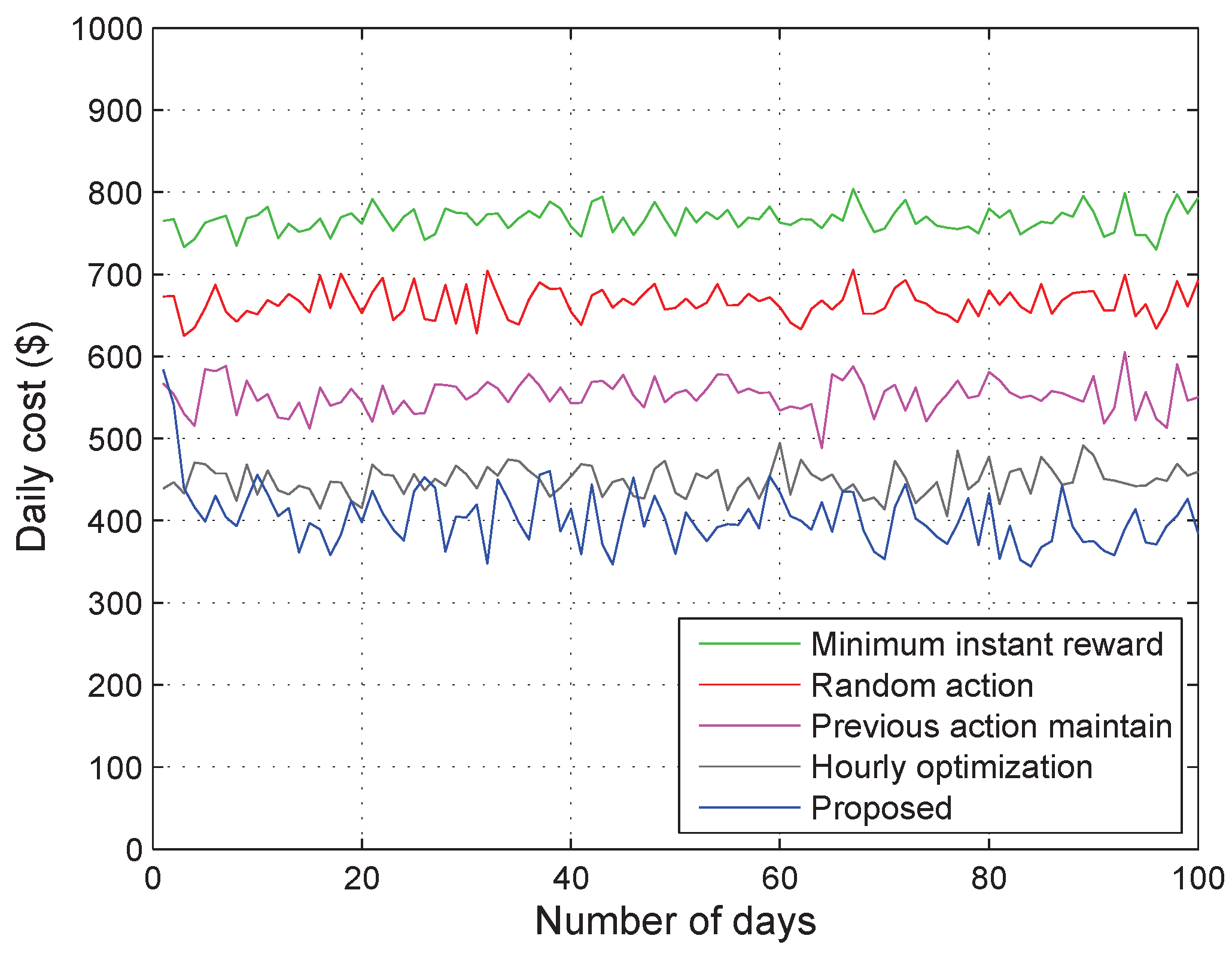
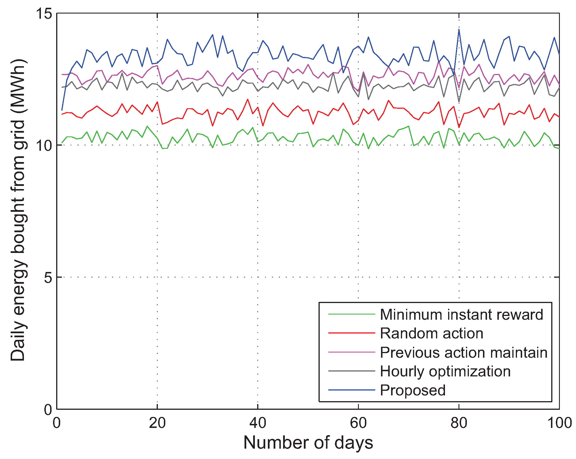
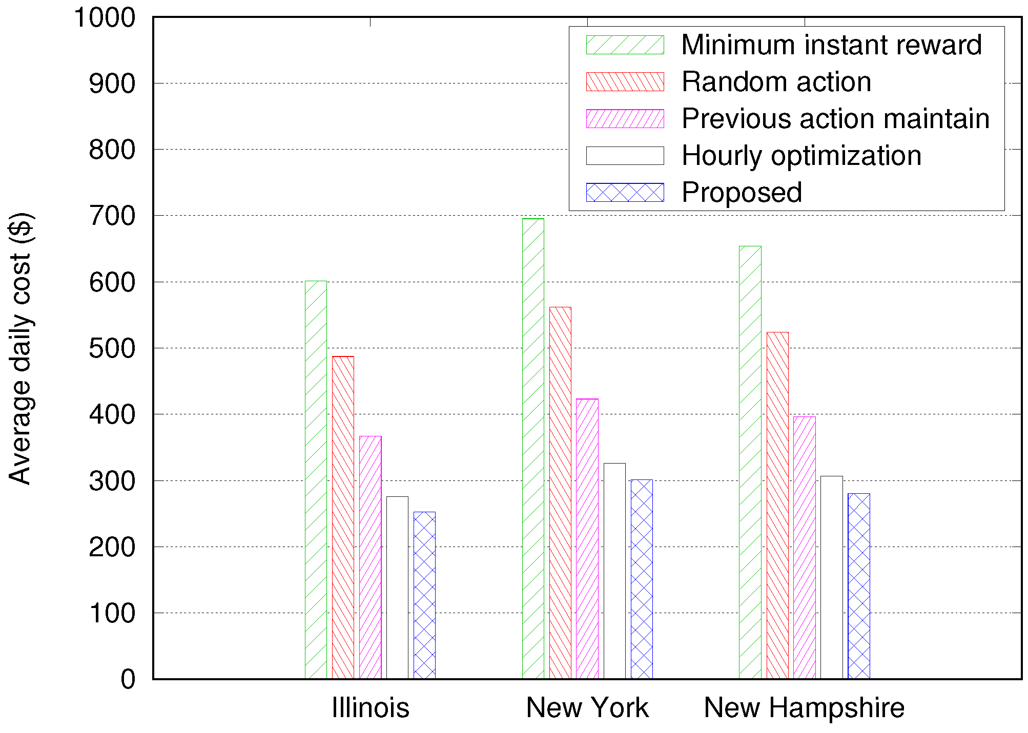
5.2. Simulation Results
- Minimum instant reward—The system always chooses the action that gives the minimum instant reward in the present time step t, without considering future rewards. This algorithm is expected to provide similar results as the proposed algorithm with .
- Random action—The action is selected randomly from the possible action set , regardless of the value of .
- Previous action maintain—This algorithm tries to always maintain its previous action while keeping the SoC of the ESS () between ()% and ()% of the maximum capacity of the ESS (), regardless of any other information on the current state. Here, is set to 20 so that is kept between 30% and 70% of . For example, if the previous action is Buying or Charging with between 30% and 70%, the algorithm keeps selecting the Buying or Charging action until reaches 70%; then, it changes the action to Selling or Discharging.
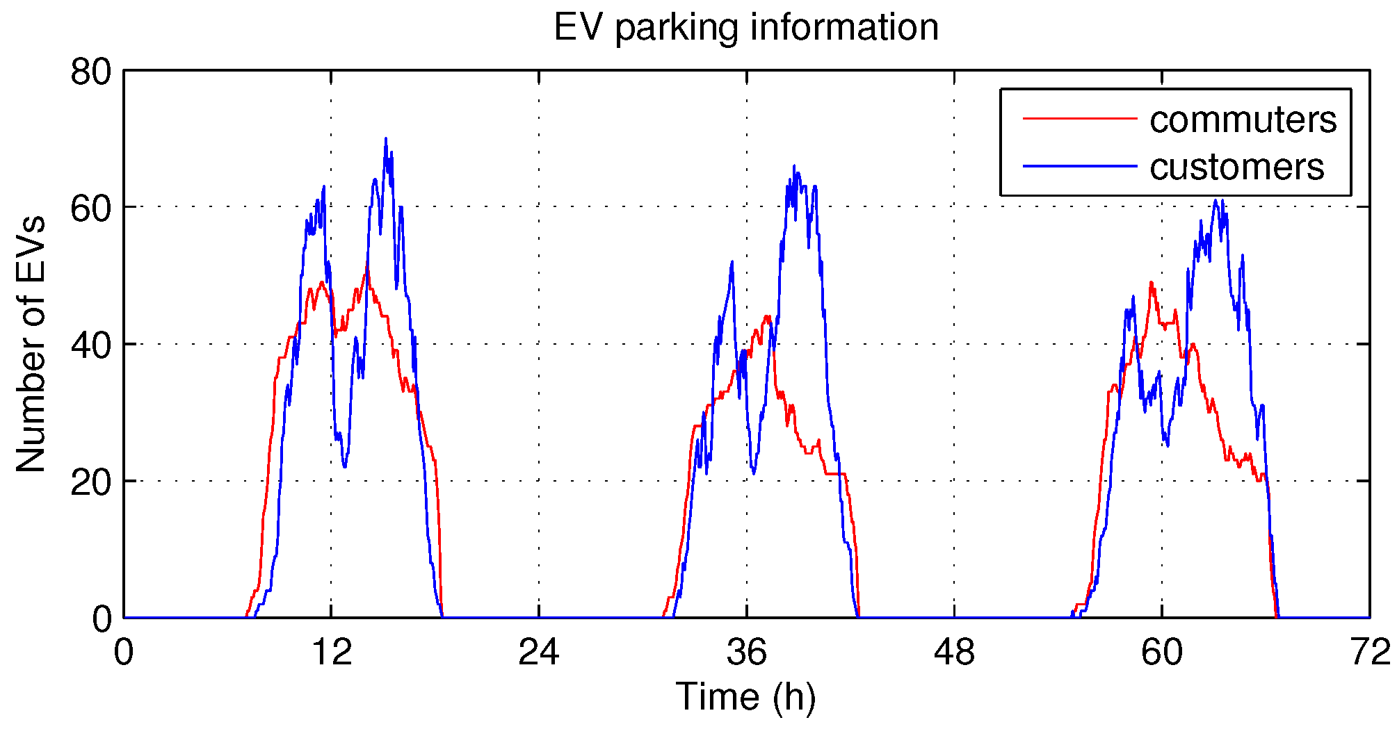
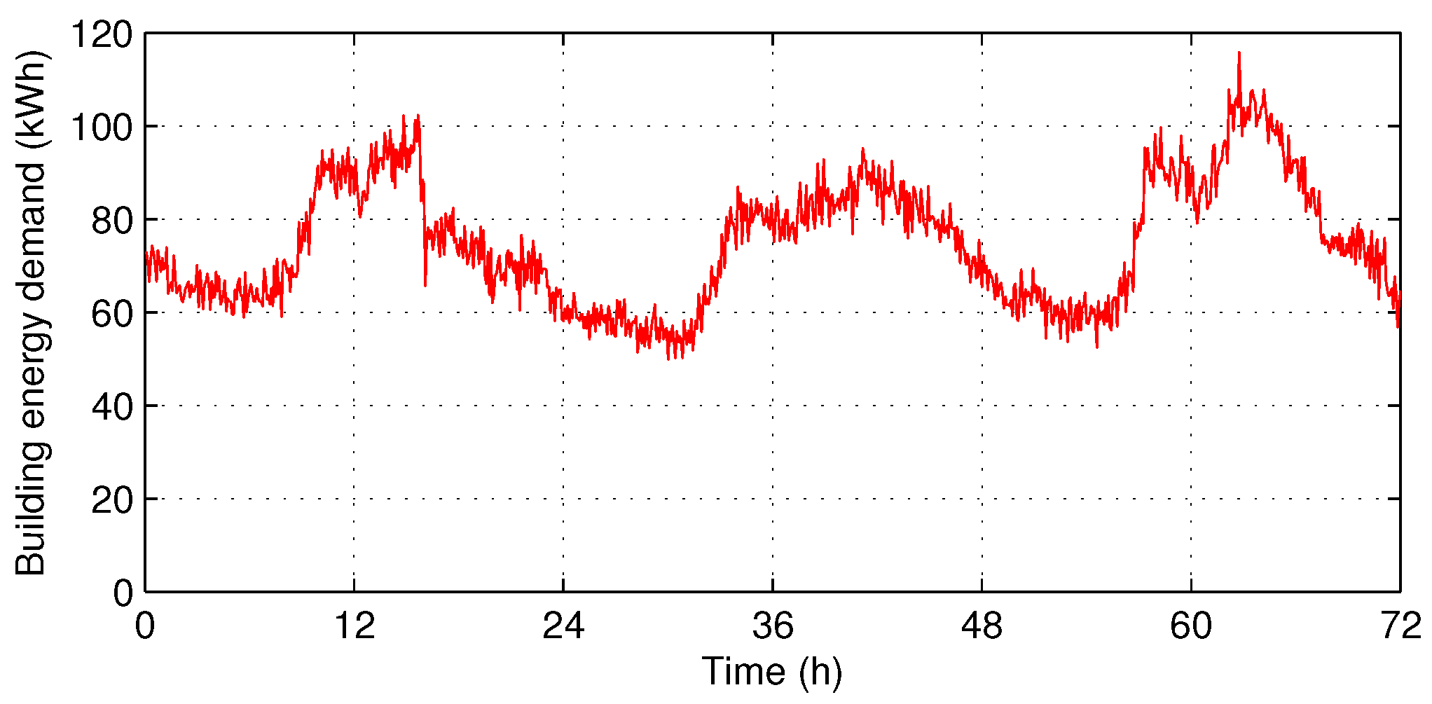
- Hourly optimization in [21]—At the beginning of every hour, this algorithm schedules the energy dispatch by using the hourly forecasted profiles. We assume that the hourly profiles of building demand (Figure 3) and PV generation (Figure 4) are given an hour in advance with Normalized Root-Mean-Square Error (NRMSE) of % and %, respectively, as in [21].
6. Conclusions and Discussion
Author Contributions
Acknowledgments
Conflicts of Interest
References
- Hashmi, M.; Hänninen, S.; Mäki, K. Survey of smart grid concepts, architectures, and technological demonstrations worldwide. In Proceedings of the IEEE PES Conference on Innovative Smart Grid Technologies (ISGT), Medellin, Colombia, 19–21 October 2011. [Google Scholar]
- Palensky, P.; Dietrich, D. Demand side management: Demand response, intelligent energy systems, and smart loads. IEEE Trans. Ind. Inform. 2011, 7, 381–388. [Google Scholar] [CrossRef]
- Kara, E.C.; Berges, M.; Krogh, B.; Kar, S. Using smart devices for system-level management and control in the smart grid: A reinforcement learning framework. In Proceedings of the IEEE International Conference on Smart Grid Communications (SmartGridComm), Tainan, Taiwan, 5–8 November 2012. [Google Scholar]
- Ruelens, F.; Claessens, B.J.; Vandael, S.; De Schutter, B.; Babuška, R.; Belmans, R. Residential demand response of thermostatically controlled loads using batch reinforcement learning. IEEE Trans. Smart Grid 2016, 8, 2149–2159. [Google Scholar] [CrossRef]
- Ju, C.; Wang, P.; Goel, L.; Xu, Y. A two-layer energy management system for microgrids with hybrid energy storage considering degradation costs. IEEE Trans. Smart Grid 2017. [Google Scholar] [CrossRef]
- Kuznetsova, E.; Li, Y.F.; Ruiz, C.; Zio, E.; Ault, G.; Bell, K. Reinforcement learning for microgrid energy management. Energy 2013, 59, 133–146. [Google Scholar] [CrossRef]
- Choi, J.; Shin, Y.; Choi, M.; Park, W.K.; Lee, I.W. Robust control of a microgrid energy storage system using various approaches. IEEE Trans. Smart Grid 2018. [Google Scholar] [CrossRef]
- Farzin, H.; Fotuhi-Firuzabad, M.; Moeini-Aghtaie, M. A stochastic multi-objective framework for optimal scheduling of energy storage systems in microgrids. IEEE Trans. Smart Grid 2017, 8, 117–127. [Google Scholar] [CrossRef]
- He, Y.; Venkatesh, B.; Guan, L. Optimal scheduling for charging and discharging of electric vehicles. IEEE Trans. Smart Grid 2012, 3, 1095–1105. [Google Scholar] [CrossRef]
- Honarmand, M.; Zakariazadeh, A.; Jadid, S. Optimal scheduling of electric vehicles in an intelligent parking lot considering vehicle-to-grid concept and battery condition. Energy 2014, 65, 572–579. [Google Scholar] [CrossRef]
- Shi, W.; Wong, V.W. Real-time vehicle-to-grid control algorithm under price uncertainty. In Proceedings of the IEEE International Conference on Smart Grid Communications (SmartGridComm), Brussels, Belgium, 17–20 October 2011. [Google Scholar]
- Di Giorgio, A.; Liberati, F.; Pietrabissa, A. On-board stochastic control of electric vehicle recharging. In Proceedings of the IEEE Conference on Decision and Control (CDC), Florence, Italy, 10–13 December 2013. [Google Scholar]
- U.S. Energy Information Administration (EIA). International Energy Outlook 2016. Available online: https://www.eia.gov/outlooks/ieo/buildings.php (accessed on 3 March 2018).
- Zhao, P.; Suryanarayanan, S.; Simões, M.G. An energy management system for building structures using a multi-agent decision-making control methodology. IEEE Trans. Ind. Appl. 2013, 49, 322–330. [Google Scholar] [CrossRef]
- Wang, Z.; Yang, R.; Wang, L. Multi-agent control system with intelligent optimization for smart and energy-efficient buildings. In Proceedings of the IEEE Conference on Industrial Electronics Society (IECON), Glendale, AZ, USA, 7–10 November 2010. [Google Scholar]
- Wang, Z.; Wang, L.; Dounis, A.I.; Yang, R. Integration of plug-in hybrid electric vehicles into energy and comfort management for smart building. Energy Build. 2012, 47, 260–266. [Google Scholar] [CrossRef]
- Missaoui, R.; Joumaa, H.; Ploix, S.; Bacha, S. Managing energy smart homes according to energy prices: Analysis of a building energy management system. Energy Build. 2014, 71, 155–167. [Google Scholar] [CrossRef]
- Basit, A.; Sidhu, G.A.S.; Mahmood, A.; Gao, F. Efficient and autonomous energy management techniques for the future smart homes. IEEE Trans. Smart Grid 2017, 8, 917–926. [Google Scholar] [CrossRef]
- Wang, F.; Zhou, L.; Ren, H.; Liu, X.; Talari, S.; Shafie-khah, M.; Catalão, J.P. Multi-objective optimization model of source-load-storage synergetic dispatch for a building energy management system based on TOU price demand response. IEEE Trans. Ind. Appl. 2018, 54, 1017–1028. [Google Scholar] [CrossRef]
- Yan, Q.; Zhang, B.; Kezunovic, M. Optimized operational cost reduction for an EV charging station integrated with battery energy storage and PV generation. IEEE Trans. Smart Grid 2018. [Google Scholar] [CrossRef]
- Di Piazza, M.; La Tona, G.; Luna, M.; Di Piazza, A. A two-stage energy management system for smart buildings reducing the impact of demand uncertainty. Energy Build. 2017, 139, 1–9. [Google Scholar] [CrossRef]
- Sutton, R.S.; Barto, A.G. Reinforcement Learning: An Introduction; MIT Press: Cambridge, MA, USA, 1998. [Google Scholar]
- Manandhar, U.; Tummuru, N.R.; Kollimalla, S.K.; Ukil, A.; Beng, G.H.; Chaudhari, K. Validation of faster joint control strategy for battery-and supercapacitor-based energy storage system. IEEE Trans. Ind. Electron. 2018, 65, 3286–3295. [Google Scholar] [CrossRef]
- Burger, S.P.; Luke, M. Business models for distributed energy resources: A review and empirical analysis. Energy Policy 2017, 109, 230–248. [Google Scholar] [CrossRef]
- Mao, T.; Lau, W.H.; Shum, C.; Chung, H.S.H.; Tsang, K.F.; Tse, N.C.F. A regulation policy of EV discharging price for demand scheduling. IEEE Trans. Power Syst. 2018, 33, 1275–1288. [Google Scholar] [CrossRef]
- Kearns, M.; Singh, S. Near-optimal reinforcement learning in polynomial time. Mach. Learn. 2002, 49, 209–232. [Google Scholar] [CrossRef]
- Research Institute for Solar and Sustainable Energies (RISE). Available online: https://rise.gist.ac.kr/ (accessed on 15 February 2018).
- Gwangju Buk-Gu Office. Available online: http://eng.bukgu.gwangju.kr/index.jsp (accessed on 12 March 2018).
- Energy Price Table by Korea Electric Power Corporation (KEPCO). Available online: http://cyber.kepco.co.kr/ckepco/front/jsp/CY/E/E/CYEEHP00203.jsp (accessed on 17 March 2018).
- ISO New England. Available online: https://www.iso-ne.com/ (accessed on 28 March 2018).


| Name | Values |
|---|---|
| Length of time step | (min) |
| ESS capacity | (kWh) |
| ESS guard ratio | |
| Initial SoC of ESS | (kWh) |
| Energy unit for Charging and Selling | (kWh) |
| Learning rate | |
| Discount factor | |
| -greedy parameter |
© 2018 by the authors. Licensee MDPI, Basel, Switzerland. This article is an open access article distributed under the terms and conditions of the Creative Commons Attribution (CC BY) license (http://creativecommons.org/licenses/by/4.0/).
Share and Cite
Kim, S.; Lim, H. Reinforcement Learning Based Energy Management Algorithm for Smart Energy Buildings. Energies 2018, 11, 2010. https://doi.org/10.3390/en11082010
Kim S, Lim H. Reinforcement Learning Based Energy Management Algorithm for Smart Energy Buildings. Energies. 2018; 11(8):2010. https://doi.org/10.3390/en11082010
Chicago/Turabian StyleKim, Sunyong, and Hyuk Lim. 2018. "Reinforcement Learning Based Energy Management Algorithm for Smart Energy Buildings" Energies 11, no. 8: 2010. https://doi.org/10.3390/en11082010
APA StyleKim, S., & Lim, H. (2018). Reinforcement Learning Based Energy Management Algorithm for Smart Energy Buildings. Energies, 11(8), 2010. https://doi.org/10.3390/en11082010