1. Introduction
An electric motor is a machine that converts electrical energy into mechanical movement, usually linear or rotational motion. A different motor category, that of spherical motors [
1,
2,
3,
4], include machines that produce motion along the surfaces of hemispheres. This category has been drawn much attention in the last decades due to the potential of applications [
5,
6,
7,
8]. However, the first studies on the spherical movement of the axis of an electric motor date back to the 1950s with the works of Williams et al. [
9,
10,
11] and Haeussermann et al. [
12,
13]. Since then, several interesting proposals have emerged [
14,
15,
16,
17], but the published designs are difficult to reproduce to verify the achieved results [
18,
19,
20,
21,
22,
23].
The goal of designing a spherical motor with multiple degrees of freedom (
M-DOF) that meets the requirements of real-world applications is not new [
10,
12,
24], although it is yet to be fully achieved. Current requirements encompasses basically an optimized construction process, simple and accurate positioning control system, large surface of motion, and high torque in the moving axis [
15,
25,
26,
27,
28,
29]. The possible uses for this type of motor are difficult to list, but in the literature it is possible to find applications in microsatellite control, 3D camera systems (e.g., for simulations of the ballistic movements of the human eye), prosthetics systems for wrists and joints, and in many industrial assembly tools [
7,
8,
16,
22,
30,
31,
32,
33].
Despite the large number of the aforementioned applications, they are all still restricted to academic laboratory domains. This means that, to the best of the authors’ knowledge, no spherical motor application has been reported to date within industrial settings. Possible explanations for this can be the lack of standardization in the construction design and no reliable positioning control systems. Another characteristic that may be impairing a large scale adoption of spherical motors in industrial scenarios is that the vast majorities of the design and control approaches available are very difficult to reproduce, with important construction and control details omitted.
By addressing these limitations of the current research on the design, construction and control of PM spherical motors, in this paper, we introduce a fully reproducible prototype of a permanent magnet (PM) spherical motor with two degrees of freedom (2-DOF) and three coils in the stator, providing in-depth details of its mathematical modeling, its construction and its positioning control system. In particular, the positioning system is designed as a visual servo control system, allowing the gathering of input–output data pairs to build a very accurate artificial neural network architecture [
34,
35,
36,
37,
38,
39,
40]. A comprehensive evaluation of the positioning control of the proposed model when engaged in the task of tracking a desired trajectory is reported.
The remainder of the paper is organized as follows. In
Section 2, we carefully describe the electromagnetic theory behind the modeling and design of the proposed PM spherical motor prototype. In
Section 3, we present the mathematical modeling of the positioning system and discuss the associated difficulties in turning it into a reliable (i.e., accurate) system in practice. The stator and rotor designs of the prototype motor are introduced in
Section 4. The neural network design procedures are detailed in
Section 5. Results are reported and discussed in
Section 6. The paper is concluded in
Section 7.
2. Theoretical Aspects
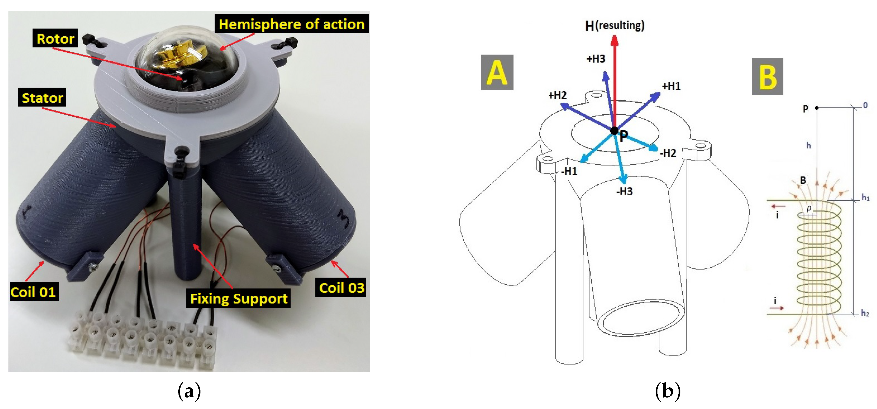
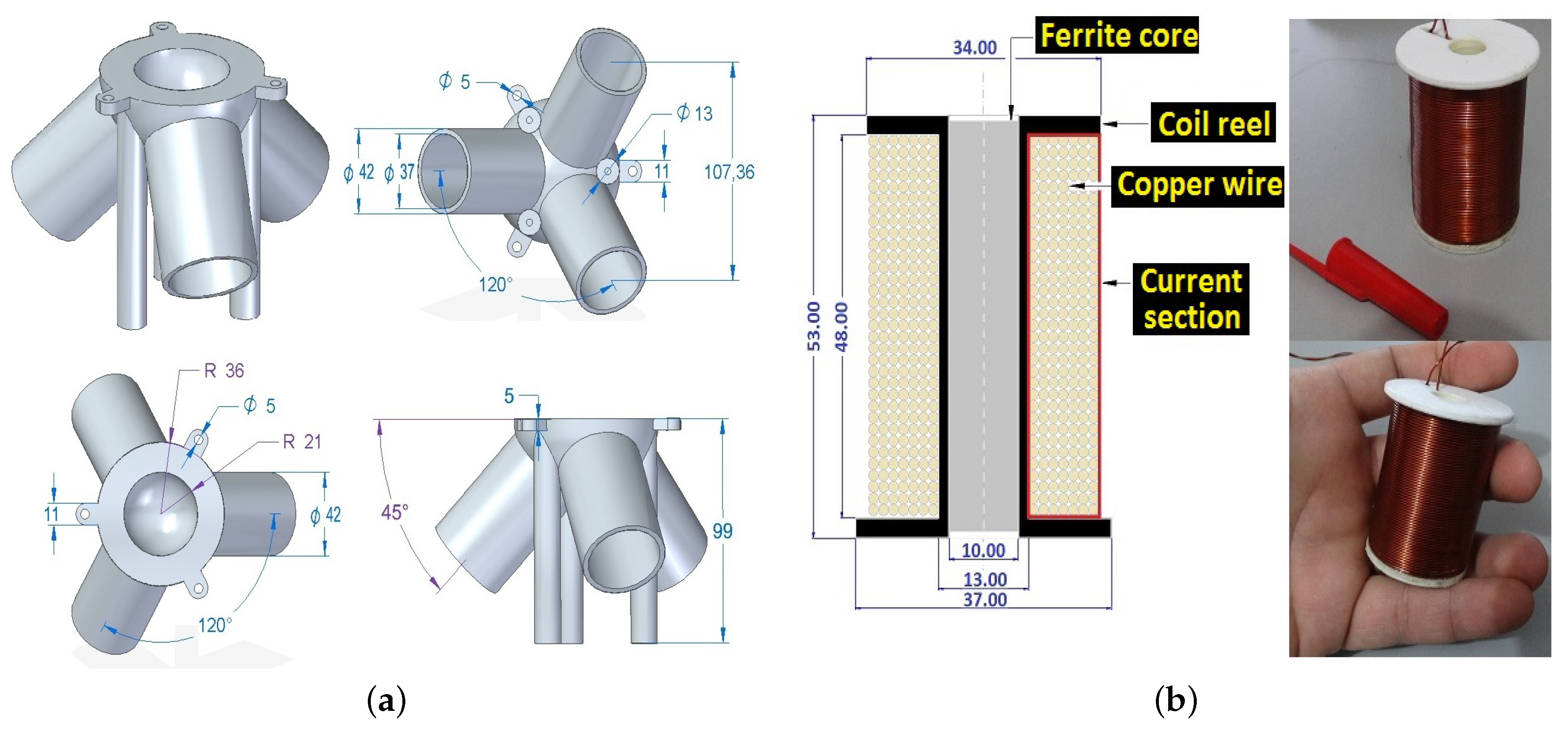
The constructed prototype motor consists of a stator with three coils, as shown in
Figure 1a. The current in each coil can be controlled independently, generating a resultant magnetic field that points to the hemisphere of action. Generally speaking, when the coils are fed with separate currents, torque is introduced into the rotor in a way that minimizes the potential energy system by forcing the rotor shaft to a hemisphere position. Even though our target motor has just three coils in the stator, we begin this section by presenting more general theoretical aspects that govern the motion of an ideal spherical motor with
N coils.
Biot–Savart’s law states that the absolute value of the magnetic field strength produced by a differential element is proportional to the product between the current intensity, the differential length, and the angle between the filament and the line connecting the filament to the point where the magnetic field is to be determined [
41]. Therefore, it is not possible to separate the current differential element, so it was necessary to use the function where the charge density in the coils does not depend on the time, which is the application of a constant current. By the continuity equation or by applying the divergence theorem, it is shown that the total current circulating in a closed circuit is zero. Mathematically, we have
and
Thus, the integral form of
Biot–Savart’s law [
6,
42] is given by
Based on Equation (
3), while
H is the magnetic field strength, Id
L is the current differential element and R the distance of the current differential element to the point of the field. The magnetic field generated by the coils pointing to the center of the stator was determined, being concentric to the rotor, as shown in
Figure 1b. The goal is to determine the magnetic field at the center of the sphere, the location on which the resulting field determines the magnetic dipole moment in the rotor.
The magnetic field in the point
P, due to a turn of radius
and located at a distance
h situated on an axis on the same plane that is normal, is given by
where
h is the height of the coil (
= beginning,
= end) (m),
is the coil radius (
= outside,
= inside) (m),
I is the current in the wire section (A), and
is unit vector in the direction of the
z-axis.
For a coil (see
Figure 1b), we obtain
where
is the surface current density (A/m
),
is the radius of the wire used in the coil (m), and
is the unit vector associated to the
i-th coil. The direction of the field
H is obtained by the right hand rule for a current
I that circulates in the coil [
43].
In general, by considering k coils for the rotor of a spherical actuator, at an instant of time () the coils generate a resultant magnetic field passing through the center of the stator. If this resultant vector is sufficient to overcome the inertia of the rotor, it will drive the rotor axis to a certain point in the hemisphere.
The resulting field is in the direction of
, with
,
, denoting the current of the
i-th coil. Thus, the intensity of the resulting magnetic field passing through the center of the stator is given either by
or by
with
C defined as
where sinh is the hyperbolic sin function;
and
are, respectively, the useful height and radius of the coil (m); and
is the coil packing factor
.
For the spherical system of interest, the
k coils are at the same distance
h to the center of the spherical rotor, which corresponds to the radius of the rotor. To locate each coil of the rotor, the spherical coordinate system is used as a function of the angles
and
. The resulting magnetic field is then given by
where this linear combination, taking as weights the currents in each coil, generates a direction which depends on constructive factors, such as the position of each coil.
The magnitude
H of the magnetic field vector at the center of the rotor is given by
with the respective projections of
onto the Cartesian axes written as
and
Let
be the resultant magnetic field departing from the center of the rotor and that points towards the hemisphere of action (see
Figure 1b). Then, the intensity of the magnetic field in each coordinate is linked to the current of the
k motor coils to generate the resulting field vector
. To find these currents, we start from
then we get
,
and
from Equations (
11)–(
13) and insert them into Equation (
14) to obtain
By defining the position matrix of
k coils as
we arrive at the final expression for the desired currents:
If , then is invertible and it is possible to compute the currents to drive the rotor depending solely on the positions of the coils.
3. Three-Coil Spherical Motor Positioning System
Movements of spherical motors are grounded on the electromagnetic theory; however, due to the influence of the magnetic field generated by the rotor on the resulting field of the coils, it is very difficult to analyze the dynamics of the interaction between these fields during motor operation. Furthermore, there are variables, such as friction and the weight of the rotor itself, that contribute to the nonlinearity of the system as a whole, diminishing the accuracy of the positioning control [
44].
A simplifying assumption considers that the magnetic fields of the coils are not subject to interference from the medium they are inserted or from the rotor field. For a PM spherical motor with three non-collinear coils, it is then possible to predict the position of the rotor rod by applying Equation (
17) to compute the currents (
). This is the smallest number of coils capable of driving the magnetic field toward any point in the working space. (With a single coil, it is possible to generate a field in the straight direction, passing through the origin. With two non-collinear coils, it is possible to generate resultant fields only in the plane.)
Equation (
17) can then be rewritten for the particular case of a three-coil PM spherical motor as
where
,
, denotes the unit vector in each of the Cartesian directions.
Since the positions of the coils are specifications of the motor design, the matrix
is known and given by
Since
is a real nonnegative number, as defined in Equation (
10), we can group it with
under a single real number
that represents the intensity of magnetic field vector:
In our proposed PM spherical motor design, we set . If a higher torque is required, the current in each coil can be increased, provided that it is kept within the range A 1.4 A.
Since all the positions of the coils are known with respect to the center of the system, as shown in
Figure 2a, then the inverse of the matrix
is given by
while
and
are defined as
and
The parameters
and
are the desired angles of the rotor axis. Then, the currents
,
and
, required to drive the rotor axis to those angles can now be computed as
resulting in the following set of individual equations for each coil’s current:
Remark 1. When performing the first tests with the built prototype motor, it was observed that the position setpoint (i.e., the desired position in the hemisphere) was not successfully reached. The hypothesis formulated was that this was result of elements ignored in the modeling, such as the friction in the bearings of the cardan system, the weight of the rod attached to the axis of motion, and the influence of the permanent magnet of the rotor in the magnetic field generated by the coils (stator).
Remark 2. Instead of revising the modeling assumptions that led to linear system in Equation (24), it was decided to handle nonlinearity and unmodeled issues by gathering data in the form of input–output pairs to train a nonlinear neural network model as part of a visual servo control system. This approach has considerably increased the accuracy of the motor in reaching the set-points. Details on the training and testing of the neural network model are given later on this paper. 4. Stator and Rotor Design
The spherical rotor is formed by a permanent magnet and is able to rotate freely within the stator cavity, which has three coils that can independently control the magnetic field intensity applied to the rotor. The proposed design has a two-pole spherical rotor, whose goal is to drive a rod to a given position in the hemisphere and, if necessary, to follow a sequence of points of a given trajectory. When the coils are fed with different current intensities, a torque in the rotor arises in a way that minimizes the potential energy system and then controls the position of the actuator (the rod). The dimensions of the prototype, shown in
Figure 2a, were limited by the manufacturing constraints of the laboratory. The coils, shown in
Figure 2b, were designed to fit to the maximum space available in the stator to maximize the field generated with the operating current range to obtain the highest torques possible. As expected for a real-world prototype, some design (or construction) variables were kept within limits imposed by the manufacturing process, being referred to in this work as
specific design limiting dimensions (SDLD).
The developed stator has three coils arranged symmetrically in the hemisphere of the stator. The coils are positioned to form angles of degrees between each other. The goal is to design a model that is compact and that generates the largest magnetic field in the center of the rotor using the minimum number of coils. The coils are positioned symmetrically as follows: Coil 01 degrees, degrees), Coil 02 ( degrees, degrees), and Coil 03 ( degrees, degrees). The stator and coils’ reels were designed in a 3D CAD software and saved in the STL (stereolithography) file format, to be subsequently built with deposition of Polylactic Acid or Polylactide (PLA) compounds using a 3D printer.
Considering the length of the coil (
ℓ) much larger than its diameter (
d), the inductance of the coil is maximized
where
L is the inductance (in Henry ( H)),
is the permeability of free space,
N is the number of turns of the coil,
A is the area of the transversal section of the wire (in mm
),
ℓ is the length of coil (in mm), and
d is the coil diameter (in mm).
With the coils located symmetrically in a hemisphere, they generate sufficient magnetic field to drive the rotor. Each coil has been designed in accordance with the SDLD; for example, the inner diameter of the coil (13 mm) is limited by the ferrite core (Ferrite-NBC-10/50-IP6) and the respective reel, as shown in
Figure 2b. Another SDLD is the outer diameter of the coil, because the surface that the coils can occupy corresponds to a hemisphere of the stator.
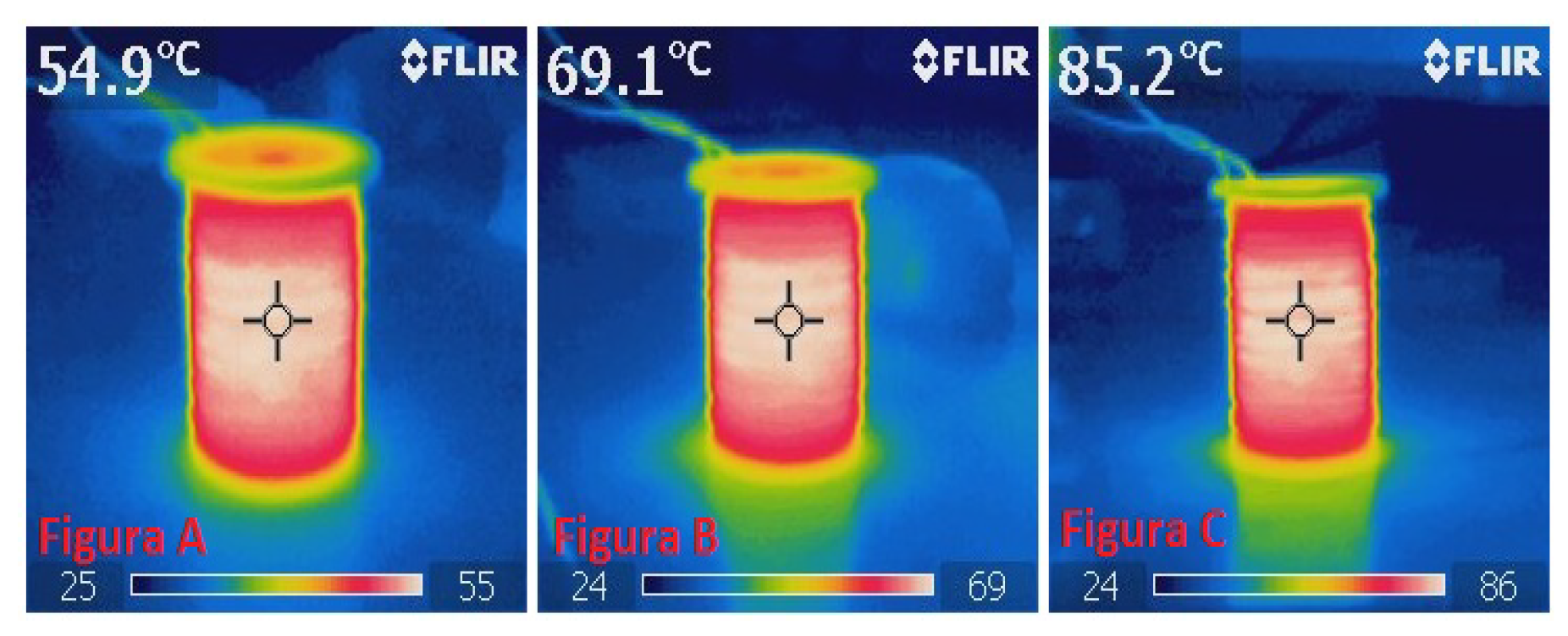
Considering the need for a high current density
×
, the copper wire that met the design specification was AWG 21. The material of the motor structure was thermoplastic (PLA), which has a glass transition temperature of 80 °C. Tests to determine the maximum temperature in the coil were performed, with the temperatures reached indicated in
Figure 3, stabilizing at 85
C for a constant current of 1.2 A. It was possible to maintain a temperature around 50 °C, with the use of a cooler on the bottom of the motor, allowing continuous operation with the maximum current.
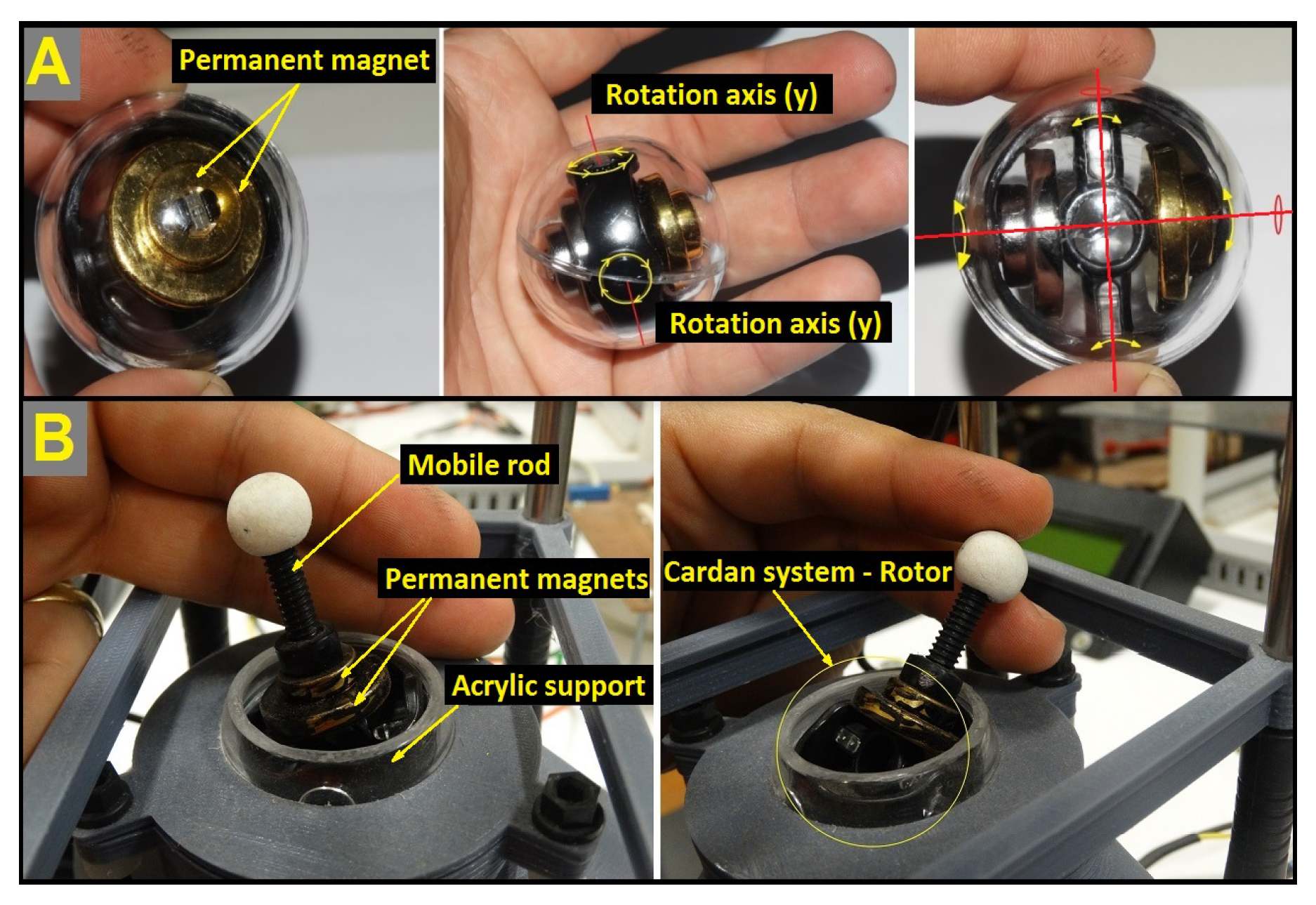
The rotor used is formed by a Neodymium-type permanent magnet, which is attached to a cardan system and can be positioned at any part of the hemisphere. The mobile rotor structure is specified as in [
45] and is comprised of four Neodymium magnets (
with grid N52) on a cardan support, which enables movement around the center of the sphere. The rotor has a diameter of 32 mm, size compared to the human eyeball (
Figure 4A). In this system, a rod was placed, making it possible to point to any point in the upper hemisphere of the sphere (
Figure 4B).
5. Neural Network Design: Data Acquisition and Training
There are several proposals in the literature for driving the rotor rod to a certain position [
46,
47,
48,
49,
50,
51,
52,
53,
54] with different degrees of accuracy reported. We chose to develop a neural network based on the visual servo control approach to achieve high accuracy.
An important component of this visual servo system is the camera located at the top of the structure shown in
Figure 5a. The camera feeds an image recognition (available in the Image Processing Toolbox of Matlab) algorithm capable of locating the position of the end-effector of the rod (a small white sphere) in the image. The camera is positioned at the minimum height from which it is possible to visualize the whole working surface of the rotor (see
Figure 5a).
The extremity of the rod (i.e., the end-effector) moves along a surface of a hemisphere. Thus, the camera system is calibrated so that the detection algorithm is able to estimate the coordinates vector of the center of the white ball in the image at a given sampling instant n. Each coordinate vector is then associated with the currents of the coils that keeps the rotor’s rod at that position.
Once the coordinate vector
is obtained, it is possible to compute the corresponding spherical coordinates
of the rotor using the following equations:
A computer is programmed to vary the PWM (Pulse-width modulation) of the driver circuit LMD18200, that regulates the current in the coils to generate the magnetic field that drives the rotor’s rod. Therefore, the spherical motor controller is composed by a H-bridge power drive and a control board (see
Figure 5b). The data acquisition system used in this work is illustrated in
Figure 5c. At a given instant
n, the camera captures an image and locates the position
of the center of the white sphere, then computes the corresponding spherical coordinates
and, finally, associates it to the applied currents
at that time instant.
To achieve the desired level of accuracy in positioning the rotor’s rod, it is necessary to gather as many data pairs
as possible. For this purpose, several image points
are uniformly sampled within the camera’s view of the rotor, as shown in
Figure 5a. In the current work, the rotor was driven to
positions within its workspace, resulting in the same number of input–output pairs
to train the neural network model.
The Neural Network Topology
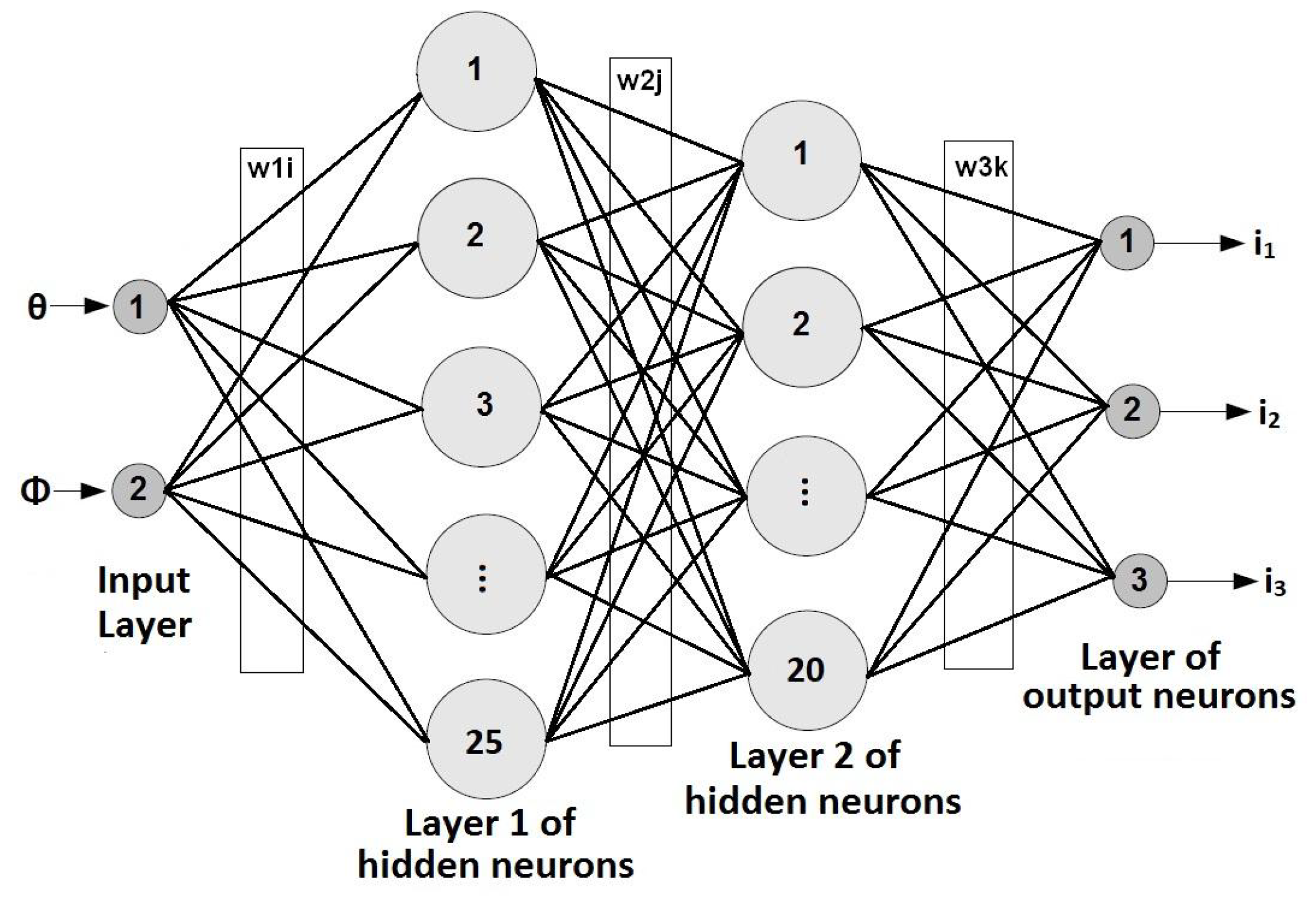
Once the data acquisition phase is completed, the next step is to train the neural network model. For this purpose, it was decided to use a multilayer Perceptron (MLP) network due to its universal approximation properties and for its flexibility in testing different topologies for the same problem. The inputs of the MLP network are the spherical coordinates
, while the outputs are the three currents of the coils (see
Figure 6).
After a period of experimentation with the data, the topology adopted was a two-hidden-layered MLP with 25 neurons in the first and 20 neurons in the second hidden layer, or just MLP (2, 25, 20, 3) for short. This network topology was trained with the standard error backpropagation algorithm using 70% of the data, while the remaining 30% was used for testing. The cost function for training and testing the MLP was the mean square error (MSE), defined as
in which
is the error of the
k-th output neuron in iteration
t. The Widrow–Hoff (also known as the least mean squares (LMS)) learning rule was used for weight updating purposes. For this gradient descent based rule, the learning rate was set to 0.001. Hidden and output neurons used the hyperbolic tangent as activation function [
55].
The training–testing procedure was repeated for 100 independent runs, so that all evaluation metrics reported in this paper are averaged results. The steps are described in Algorithm 1.
Once the neural network is trained and validated (numerical results are reported in the next section), the camera is then removed and the motor is ready to be operated under the command of the neural network. For this purpose, at a given instant n, the desired spherical coordinates of the rotor is fed to the neural network as setpoints. The network then estimates the currents of the three stator coils, which will then be produced by the driver circuitry of the motor.
The neural network design procedure just described has been successfully used in the field of intelligent robotics for building adaptive visuomotor control systems (see, for example, [
56] and references therein for a survey). As shown and discussed in the next section, this approach was able to model accurately the underlying nonlinear phenomena inherent to the design of the proposed spherical motor, a feature that was not possible by using the linear approach in Equation (
24). The dataset and the drawings (in STL file format for 3D printing) of the stator and the coil reel are available to interested readers under request.
| Algorithm 1 Two-hidden-layered MLP Training. |
STEP 1: Define the inputs (, ) and the outputs (), number of hidden layers (), number of neurons in each hidden layer and (), learning rate = . STEP 2: Separate randomly 80% of the data for training and 20% for testing. Initialize randomly all the weights and biases. STEP 3: Train the MLP (2, 25, 20, 3) network for 5000 epochs using the standard backprop algorithm (i.e., gradient descent learning without momentum term). STEP 4: Once the training phase is finished, estimate the outputs (currents: ) using the test input data. STEP 5: Compute the corresponding residuals (i.e., prediction errors) and, hence, the MSE value for testing data, as defined in Equation ( 31). STEP 6: Repeat Steps 3–5 for 100 runs (i.e., training-testing cycle). STEP 7: Compute the statistics of MSE values (average, median, standard deviation, minimum, maximum) for the 100 independent rounds. STEP 8: Store the weights and bias of the trained for posterior use by the spherical motor.
|
6. Results and Discussion
In this section, the numerical results of a comprehensive performance evaluation of the proposed PM spherical motor is presented, in particular of its positioning control system. The software of the computer vision system for data acquisition was developed using the Image Processing toolbox of Matlab. The MLP network was implemented from scratch using the script language of Matlab, i.e., the Neural Networks toolbox was not used.
6.1. Preliminary Experiments
Despite having some prior knowledge of the degree of complexity of the approximation task, we decided to initiate our quest for the best approximation model from very simple neural architectures. Hence, the first step was to evaluate the performance of a linear neural network model, the Adaline [
57], which is basically a MLP with no hidden layer.
From the available data input–output pairs, 70% were randomly selected for training, while the remaining 30% were used for testing purposes. The number of epochs was used as the stopping criterion for training and it was set to 5000, with the reason for this high number being the lack of prior knowledge of the network performance. In this section, it can be seen that this number is considerably reduced for the final MLP architecture. As expected, due to the nonlinear nature of the phenomena at hand, the performance of the Adaline topology was far from adequate, converging to a prohibitively high approximation error level. Hence, the Adaline’s results are not reported in this paper.
The next step was then to investigate the performance a single-hidden-layered MLP using the standard backprop algorithm, as mentioned previously in this paper. This study started with a small number of hidden neurons (2), increasing this number with increments of 5. The best performance was achieved for 25 hidden neurons. Higher values did not improve significantly the performance. The achieved approximation error level for this network topology was considerably better than that achieved by the Adaline network. However, it was still not possible to confidently state that this network topology would be the best one for the task of interest.
It was finally decided to evaluate a two-hidden-layered MLP with the expectation of improving the approximation performance. This decision proved to be correct because the improvement in performance was considerable. Initially, the number of neurons in the second hidden layer was heuristically set to 25, while smaller values were also investigated. This investigation led to an optimum number of 20 for the task at hand.
6.2. Further Evaluation of the Chosen MLP Model
Once the model selection phase was complete, it was decided to understand the chosen network topology a bit better. For this purpose, the MLP (2, 25, 20, 3) network was trained for different sizes of the training set: 700 (≈18%), 1400 (≈35%), 2100 (≈53%) and the previously used 2800 samples. As expected, this training parameter affects the convergence rate of the network, as can be seen in
Figure 7, in which the MSE learning curves of the selected architecture can be seen. The best performance was achieved for the training size of 2800. For this value, the required number of training epochs was considerably reduced to 500.
The numerical results in terms of the mean squared error (MSE) after 100 independent simulations are shown in
Table 1. Values of the MSE for training and testing sets are shown in Columns 3 and 4, respectively. It can be easily seen that the higher is the number of training samples, the smaller is the MSE.
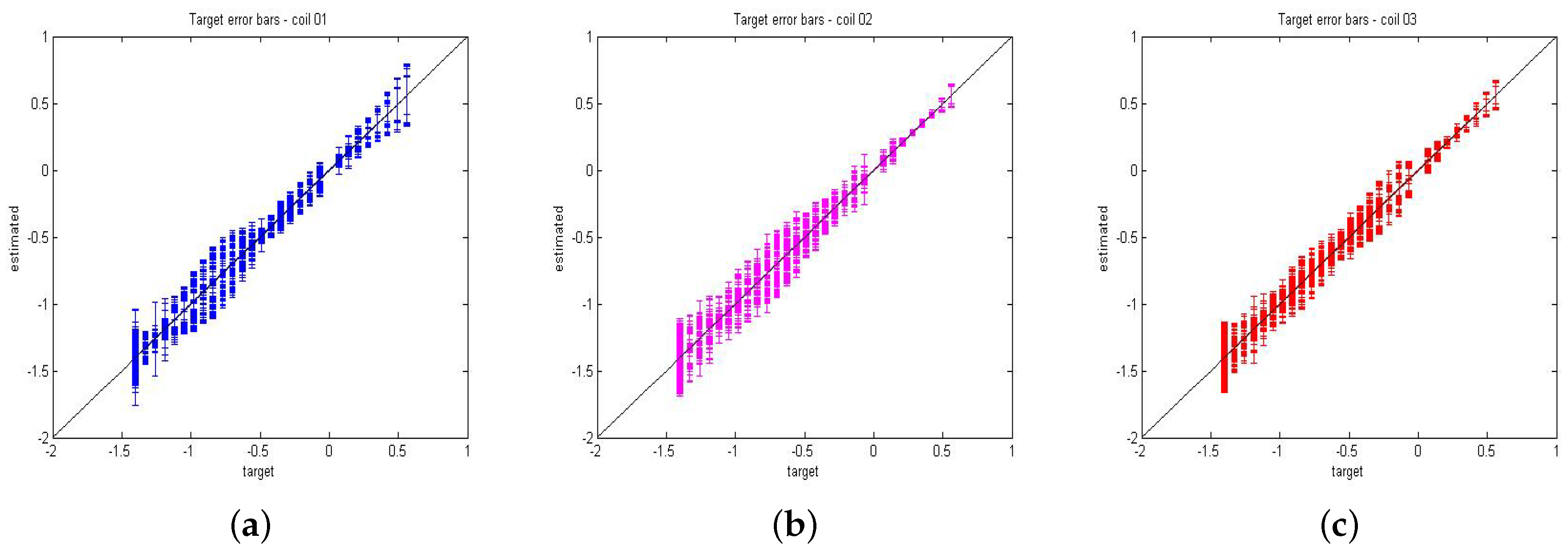
The scatterplots of the actual (i.e., target) current values versus the predicted ones for the testing dataset are shown in
Figure 8. The corresponding correlation coefficients are
(for
),
(for
) and
(for
), which indicate a very good fit of the MLP model to the data. The dispersions in the scatterplots are acceptable since the magnitude of the errors in the positioning is of tenths of millimeters due to the relatively diameter of the rotor (42 mm).
6.3. Evaluating the Chosen MLP Model on the Prototype Motor
The ultimate goal of the proposed ANN-based position control algorithm is to be used in the real prototype of the proposed spherical motor. For this purpose, among the 100 independent runs using the training set with 2800 samples, the best performing MLP(2,25,20,3) network was selected and the weights and biases determined for this network in the experiments were applied to the real spherical motor constructed
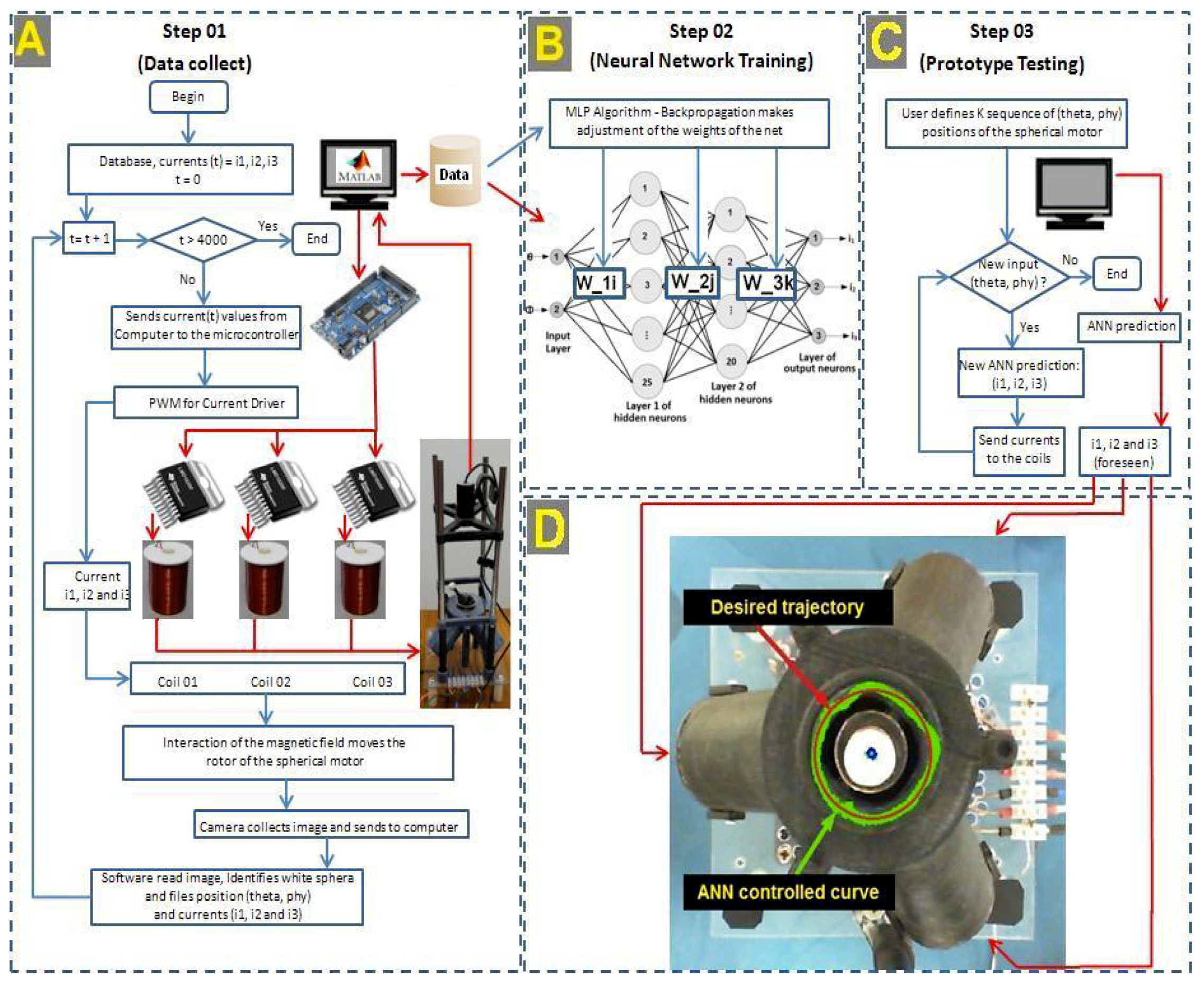
The chosen task consisted in defining a circular trajectory within the hemisphere of action of the motor’s rod and evaluate the tracking accuracy of the ANN-based position control system. A flowchart describing the sequence of steps followed by the ANN-based control algorithm during the trajectory tracking task is given in
Figure 9A–C.
For a sequence of desired positions of a given trajectory, the control algorithm estimates via the neural network the suitable values of the currents , , and and applies these values to the coils, aiming at driving the rotor’s rod to the desired spherical position. This process is repeated for each point of the trajectory.
The desired sequence of points comprising a circular trajectory was built for the angles
degrees and
ranging from 0 degrees to 360 degrees, in increments of 5 degrees. A typical execution of the position control algorithm for all the points in the trajectory resulted in the trajectory in
Figure 9D. As can be seen, the rotor’s rod, commanded by the neural network, was able to follow successfully the desired trajectory (solid line).
7. Conclusions
This paper presents all the steps that eventually led to a real-world prototype of an efficient three-pole permanent magnet spherical motor (2-DOF). The authors’ main concern was the reproducibility of the design and construction of the prototype, and, for this purpose, the details of the construction and modeling of the motor are provided. The mechanical parts of the motor were constructed by means of a 3D printer.
A particular issue addressed in this paper is the position control of the rotor, an issue commonly considered the bottleneck of the design of spherical motors. Our modeling equations, due to simplifying assumptions, such as disregarding of gravity and friction effects, did not produce accurate results. It was then decided to follow a data-driven approach by gathering input–output pairs to train a powerful nonlinear neural network model. Data acquisition was possible with the help of a camera system and an image recognition software. The camera is not used in the operation of the motor.
The neural network model was trained to receive as inputs the desired spherical coordinates of the rotor (the setpoints) and to estimate the currents in the three coils needed to reach those coordinates. This approach was successfully tested and validated by comprehensive computer simulations and also by means of a trajectory tracking task in the real prototype of the proposed spherical motor.
Currently, the author’s are working on evaluating the accuracies of other nonlinear approximation models, such as support vector regression (SVR) and the extreme learning machines (ELM), to compare their performances with the one achieved by the MLP network described in this paper.

 ,
, 


