Short-Term Load Forecasting of Natural Gas with Deep Neural Network Regression †


Opus College of Engineering, Marquette University, Milwaukee, WI 53233, USA
*
Author to whom correspondence should be addressed.
Energies 2018, 11(8), 2008; https://doi.org/10.3390/en11082008
Submission received: 29 June 2018
/
Revised: 25 July 2018
/
Accepted: 1 August 2018
/
Published: 2 August 2018
(This article belongs to the Special Issue Short-Term Load Forecasting by Artificial Intelligent Technologies)
Abstract
:Deep neural networks are proposed for short-term natural gas load forecasting. Deep learning has proven to be a powerful tool for many classification problems seeing significant use in machine learning fields such as image recognition and speech processing. We provide an overview of natural gas forecasting. Next, the deep learning method, contrastive divergence is explained. We compare our proposed deep neural network method to a linear regression model and a traditional artificial neural network on 62 operating areas, each of which has at least 10 years of data. The proposed deep network outperforms traditional artificial neural networks by 9.83% weighted mean absolute percent error (WMAPE).
1. Introduction
This manuscript presents a novel deep neural network (DNN) approach to forecasting natural gas load. We compare our new method to three approaches—a state-of-the-art linear regression algorithm and two shallow artificial neural networks (ANN). We compare our algorithm on 62 datasets representing many areas of the U.S. Each dataset consists of 10 years of training data and 1 year of testing data. Our new approach outperforms each of the existing approaches. The remainder of the introduction overviews the natural gas industry and the need for accurate natural gas demand forecasts.
The natural gas industry consists of three main parts; production and processing, transmission and storage, and distribution [1]. Like many fossil fuels, natural gas (methane) is found underground, usually near or with pockets of petroleum. Natural gas is a common byproduct of drilling for petroleum. When natural gas is captured, it is processed to remove higher alkanes such as propane and butane, which produce more energy when burned. After the natural gas has been processed, it is transported via pipelines directly to local distribution companies (LDCs) or stored either as liquid natural gas in tanks or back underground in aquifers or salt caverns. The natural gas is purchased by LDCs who provide natural gas to residential, commercial, and industrial consumers. Subsets of the customers of LDCs organized by geography or municipality are referred to as operating areas. Operating areas are defined by the individual LDCs and can be as large as a state or as small as a few towns. The amount of natural gas used often is referred to as the load and is measured in dekatherms (Dth), which is approximately the amount of energy in 1000 cubic feet of natural gas.
For LDCs, there are several uses of natural gas, but the primary use is for heating homes and business buildings, which is called heatload. Heatload changes based on the outside temperature. During the winter, when outside temperatures are low, the heatload is high. When the outside temperature is high during the summer, the heatload is approximately zero. Other uses of natural gas, such as cooking, drying clothes, and heating water and other household appliances, are called baseload. Baseload is generally not affected by weather and typically remains constant throughout the year. However, baseload may increase with a growth in the customer population.
Natural gas utility operations groups depend on reliable short-term natural gas load forecasts to make purchasing and operating decisions. Inaccurate short-term forecasts are costly to natural gas utilities and customers. Under-forecasts may require a natural gas utility to purchase gas on the spot market at a much higher price. Over-forecasts may require a natural gas utility to store the excess gas or pay a penalty.
In this paper, we apply deep neural network techniques to the problem of short term load forecasting of natural gas. We show that a moderately sized neural network, trained using a deep neural network technique, outperforms neural networks trained with older techniques by an average of 0.63 (9.83%) points of weighted mean absolute percent error (WMAPE). Additionally, a larger network architecture trained using the discussed deep neural network technique results in an additional improvement of 0.20 (3.12%) points of WMAPE. This paper is an extension of Reference [2].
The rest of the manuscript is organized as follows. Section 2 provides an overview of natural gas forecasting, including the variables used in typical forecasting models. Section 3 discusses prior work. Section 4 provides an overview of ANN and DNN architecture and training algorithms. Section 5 discusses the data used in validating our method. Section 6 describes the proposed method. Section 7 explains the experiments and their results. Section 8 provides conclusions.
2. Overview of Natural Gas Forecasting
The baseload of natural gas consumption, which does not vary with temperature for an operating area, typically changes seasonally and slowly as the number of customers, or their behavior, changes. Given the near steady nature of baseload, most of the effort in forecasting natural gas load focuses on predicting the heatload (load which varies with temperature). Hence, the most important factor affecting the natural gas load is the weather.
Figure 1 shows that natural gas load has a roughly linear relationship with temperatures above 65 °F. For this reason, it is important to consider a variety of temperature-related exogenous variables as potential inputs to short-term load forecasting models. This section discusses a few of these exogenous variables, which include heating degree day (HDD), dew point (DPT), cooling degree day (CDD), day of the week (DOW), and day of the year (DOY).
Note the kink in the trend of Figure 1 at about 65 °F. At temperatures greater than 65 °F, residential and commercial users typically stop using natural gas for heating. At temperatures greater than 65 °F, only the baseload remains. Thus, heating degree days (HDD) are used as inputs to forecasting models,
where T is the temperature, and Tref is the reference temperature [3]. Reference temperature is indicated by concatenating it to HDD, i.e., HDD65 indicates a reference temperature of 65 °F.
Several other weather-based inputs can be used in forecasting natural gas, such as wind-adjusted heating degree day (HDDW); dew point temperature (DPT), which captures humidity; and cooling degree days (CDD),
and is used to model temperature-related effects above Tref as seen in Figure 1.
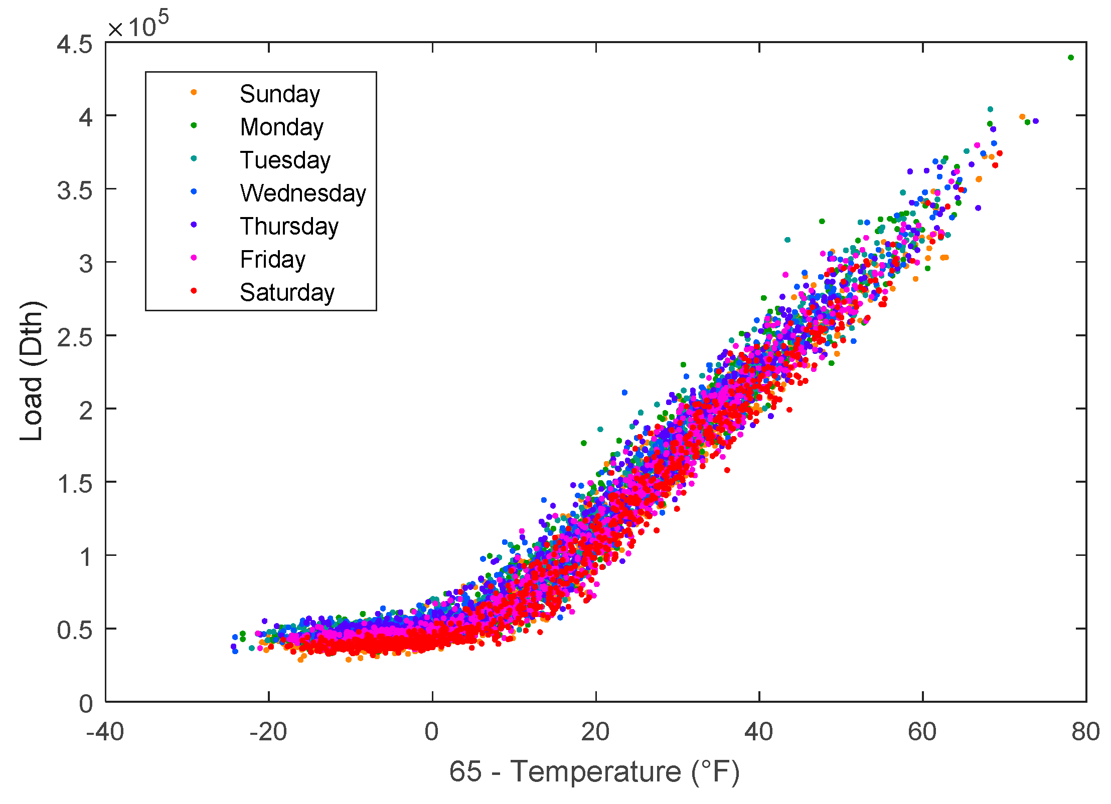
In addition to weather inputs, time variables are important for modeling natural energy demand [4]. Figure 2 illustrates the day of the week (DOW) effect. Weekends (Friday–Sunday) have less demand than weekdays (Monday–Thursday). The highest demand typically occurs on Wednesdays, while the lowest demand generally occurs on Saturdays. A day of the year (DOY) variable is also important. This allows homeowner behaviors between seasons to be modeled. In September, a 50 °F temperature will cause few natural gas customers to turn on their furnaces, while in February at 50 °F all furnaces will be on.
3. Prior Work
Multiple linear regression (LR) and autoregressive integrated moving average (ARIMA) are common models for forecasting short-term natural gas demand [5]. Vitullo et al. propose a five-parameter linear regression model [5]. Let be the day ahead forecasted natural gas demand, HDD65 be the forecasted HDD with a reference temperature of 65 °F, HDD55 be the forecasted HDD with a reference temperature 55 °F, and CDD65 be the forecasted CDD with a reference temperature 65 °F. Let ΔHDD65 be the difference between the forecasted HDD65 and the prior day’s actual HDD65. Then, Vitullo’s model is described as
β0 is the natural gas load not dependent on temperature. The natural gas load dependent on temperature is captured by the sum of β1 and β2. The two reference temperatures better model the smooth transition from heating to non-heating days. β3 accounts for recency effects [5,6]. Finally, β4 models small, but not insignificant, temperature effects during non-heating days.
While the Vitullo model and other linear models perform well on linear stationary time-series, they assume that load has roughly a linearly relationship with temperature [7]. However, natural gas demand time series is not purely linear with temperature. Some of the nonlinearities can be modeled using heating and cooling degrees, but natural gas demand also contains many smaller nonlinearities that cannot be captured easily with linear or autoregressive models even with nonlinear transformations of the data.
To address these nonlinearities, forecasters have used artificial neural networks (ANNs) in place of, or in conjunction with, linear models [5,8,9]. ANNs are universal approximators, meaning that with the right architecture, they can be used to model almost any regression problem [8]. Artificial neural networks are composed of processing nodes that take a weighted sum of their inputs and then output a nonlinear transform of that sum.
Recently, new techniques for increasing the depth (number of layers) of ANNs have yielded deep neural networks (DNN) [10]. DNNs have been applied successfully to a range of machine learning problems, including video analysis, motion capture, speech recognition, and image pattern detection [10,11].
As will be described in depth in the next section, DNNs are just large ANNs with the main difference being the training algorithms. ANNs are typically trained using gradient descent. Large neural networks trained using gradient descent suffer from diminishing error gradients. DNNs are trained using the contrastive divergence algorithm, which pre-trains the model. The pre-trained model is fine-tuned using gradient descent [12].
This manuscript adapts the DNNs to short-term natural gas demand forecasting and evaluates DNNs’ performance as a forecaster. Little work has been done in the field of time series regression using DNNs, and almost no work has been done in the field of energy forecasting with DNNs. One notable example of literature on these subjects is Qui et al., who claim to be the first to use DNNs for regression and time series forecasting [13]. They show promising results on three electric load demand time series and several other time series using 20 DNNs ensembled with support vector regression. However, the DNNs they used were quite small; the largest architecture consists of two hidden layers of 20 neurons each. Because of their small networks, Qui et al. did not take full advantage of the DNN technology.
Another example of work in this field is Busseti et al. [14], who found that deep recurrent neural networks significantly outperformed the other deep architectures they used for forecasting energy demand. These results are interesting but demonstrated poor performance when compared to the industry standard in energy forecasting, and they are nearly impossible to replicate given the information in the paper.
Some good examples of time series forecasting using DNNs include Dalto, who used them for ultra-short-term wind forecasting [15], and Kuremoto et al. [16], who used DNNs on the Competition on Artificial Time Series benchmark. In both applications, DNNs outperformed neural networks trained by backpropagation. Dalto capitalized on the work of Glorot and Bengio when designing his network and showed promising results [17]. Meanwhile, Kuremoto successfully used Kennedy’s particle swarm optimization in selecting their model parameters [18]. The work most similar to ours is Ryu et al., who found that two different types of examined DNNs performed better on short-term load forecasting of electricity than shallow neural networks and a double seasonal Holt-Winters model [19].
Other, more recent examples of work in this field include Kuo and Huang [20], who use a seven-layer convolutional neural network for forecasting energy demand with some success. Unfortunately, they do not use any weather information in their model which results in poor forecasting accuracy compared to those who do account for weather. Li et al. used a DNN combined with hourly consumption profile information to do hourly electricity demand forecasting [21]. Chen et al. used a deep residual network to do both point and probabilistic short-term load forecasting of natural gas [22]. Perhaps the most similar recent work to that which is presented in this paper is Hosein and Hosein, who compared a DNN without RBM pretraining to one with RBM pretraining on short-term load forecasting of electricity. They found that the pretrained DNN performed better, especially as network size increased [23].
Given the successful results of these deep neural network architectures on similar problems, it is expected that DNNs will surpass ANNs in many regression problems, including the short-term load forecasting of natural gas. This paper explores the use of DNNs to model a natural gas system by comparing the performance of the DNN to various benchmark models and the current state-of-the-art models.
4. Artificial and Deep Neural Networks
This section provides an overview of ANNs and DNNs and how to train them to solve regression problems. An ANN is a network of nodes. Each node sums its inputs and then nonlinearly transforms them. Let xi represent the ith input to the node of a neural network, wi the weight of the ith input, b the bias term, n the number of inputs, and o the output of the node. Then
where
This type of neural network node is a sigmoid node. However other nonlinear transforms may be used. For regression problems, the final node of the network is typically a linear node where
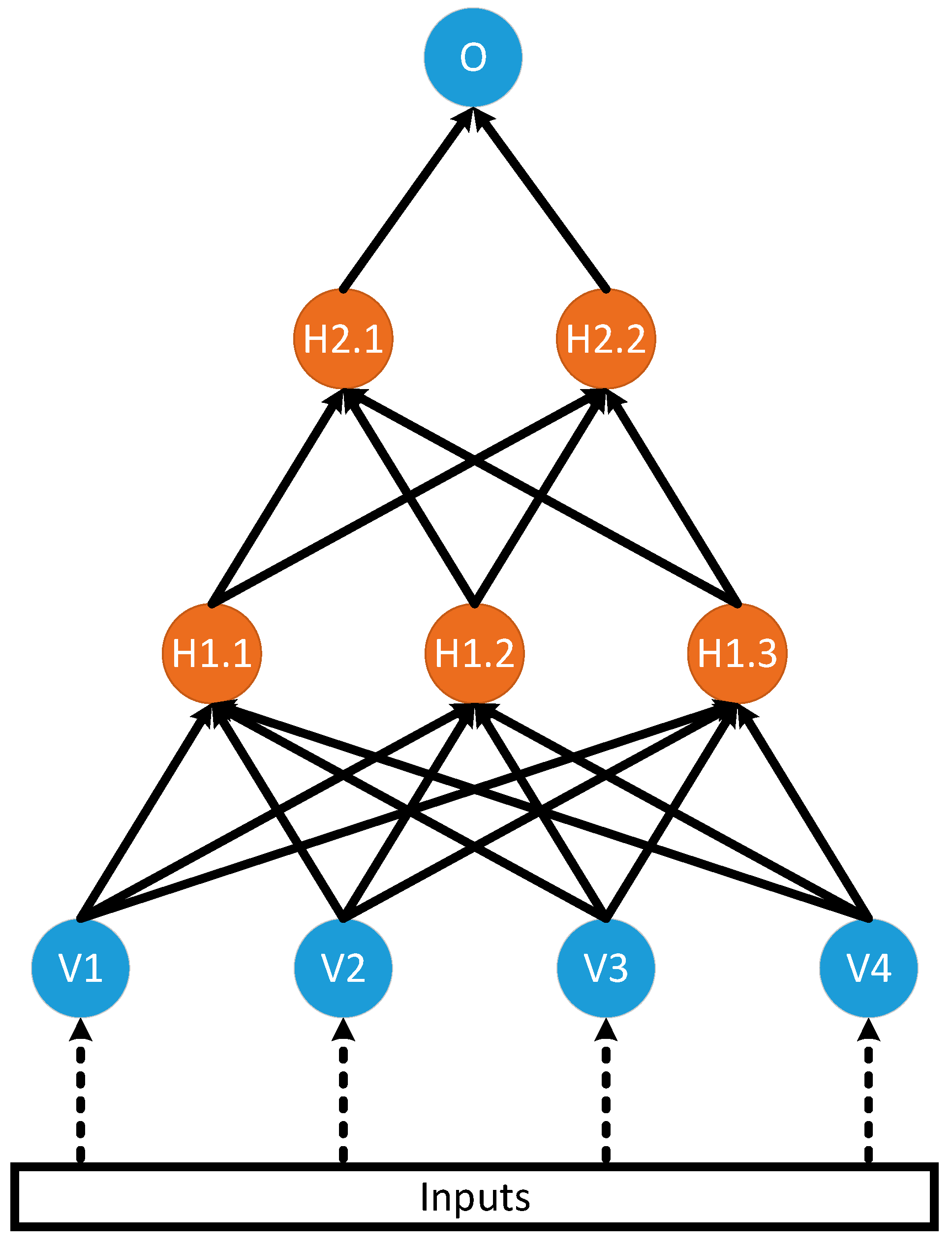
A network of nodes is illustrated in Figure 3 below for a feedforward ANN, whose outputs always connect to nodes further in the network. The arrows in Figure 3 indicate how the outputs of nodes in one layer connect to the inputs in the next layer. The visible nodes are labelled with a V. The hidden nodes are labelled with an Hx.y, where x indicates the layer number and y indicates the node number. The output node is labeled O.
The ANN is trained using the backpropagation algorithm [24]. The backpropagation algorithm is run over all the training data. This is called an epoch. When training an ANN, many epochs are performed with a termination criterion such as a maximum number of epochs or the error falling below a threshold.
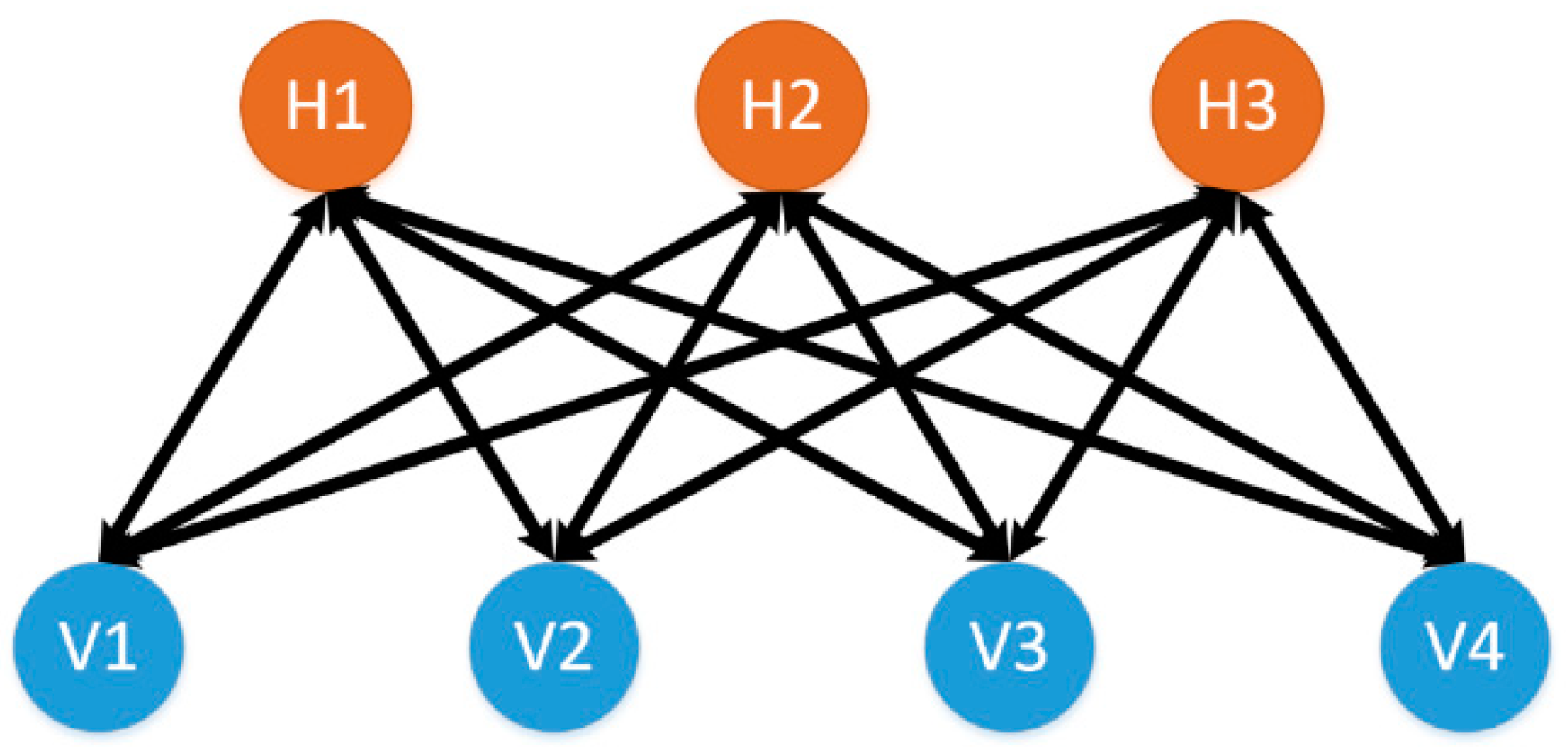
Next, we describe a DNN. A DNN is essential an ANN with many hidden layers. The difference is in the training process. Rather than training the network using only the backpropagation algorithm, an initialization phase is done using the contrastive divergence algorithm [25,26]. The contrastive divergence algorithm is performed on a restricted Boltzmann machine (RBM). Figure 4 illustrates a RBM with four visible nodes and three hidden nodes. Important to note is that unlike the ANN, the arrows point in both directions. This is to indicate that the contrastive divergence algorithm updates the weights by propagating the error in both directions.
Similar to an ANN, a RBM has bias terms. However, since the error is propagated in both directions there are two bias terms, b and c. The visible and hidden nodes are calculated from one another [26]. Let vi represent the ith visible node, wi the weight of the ith visible node, c the bias term, n the number of visible nodes, and h the hidden node.
which can be rewritten in vector notation for all hidden units as
Similarly, the visible node can be calculated in terms of the hidden nodes. Let hj represent the jth hidden node, wj the weight of the jth hidden node, b the bias term, m the number of hidden nodes, and v the visible node. Then
which can be rewritten in vector notation for all visible units as
where WT is the transpose of W.
Training a RBM is done in three phases as described in Algorithm 1 for training vector v0 and a training rate ε. Algorithm 1 is performed on iterations (epochs) of all input vectors.
| Algorithm 1: Training restricted Boltzmann machines using contrastive divergence | |
| 1 | //Positive Phase |
| 2 | h0 = σ (Wv0 + c) |
| 3 | for each hidden unit h0i: |
| 4 | if h0i > rand(0,1)//rand(0,1) represents a sample drawn from the uniform distribution |
| 5 | h0i = 1 |
| 6 | else |
| 7 | h0i = 0 |
| 8 | //Negative Phase |
| 9 | v1 = σ (WTh0 + b) |
| 10 | for each visible units v1j: |
| 11 | if v1j > rand(0,1) |
| 12 | v1j = 1 |
| 13 | else |
| 14 | v1j = 0 |
| 15 | //Update Phase |
| 16 | h1 = σ (Wv1 + c) |
| 17 | W = ε (h0v0T − h1v1T) |
| 18 | b = ε (h0 − h1) |
| 19 | c = ε (v0 − v1) |
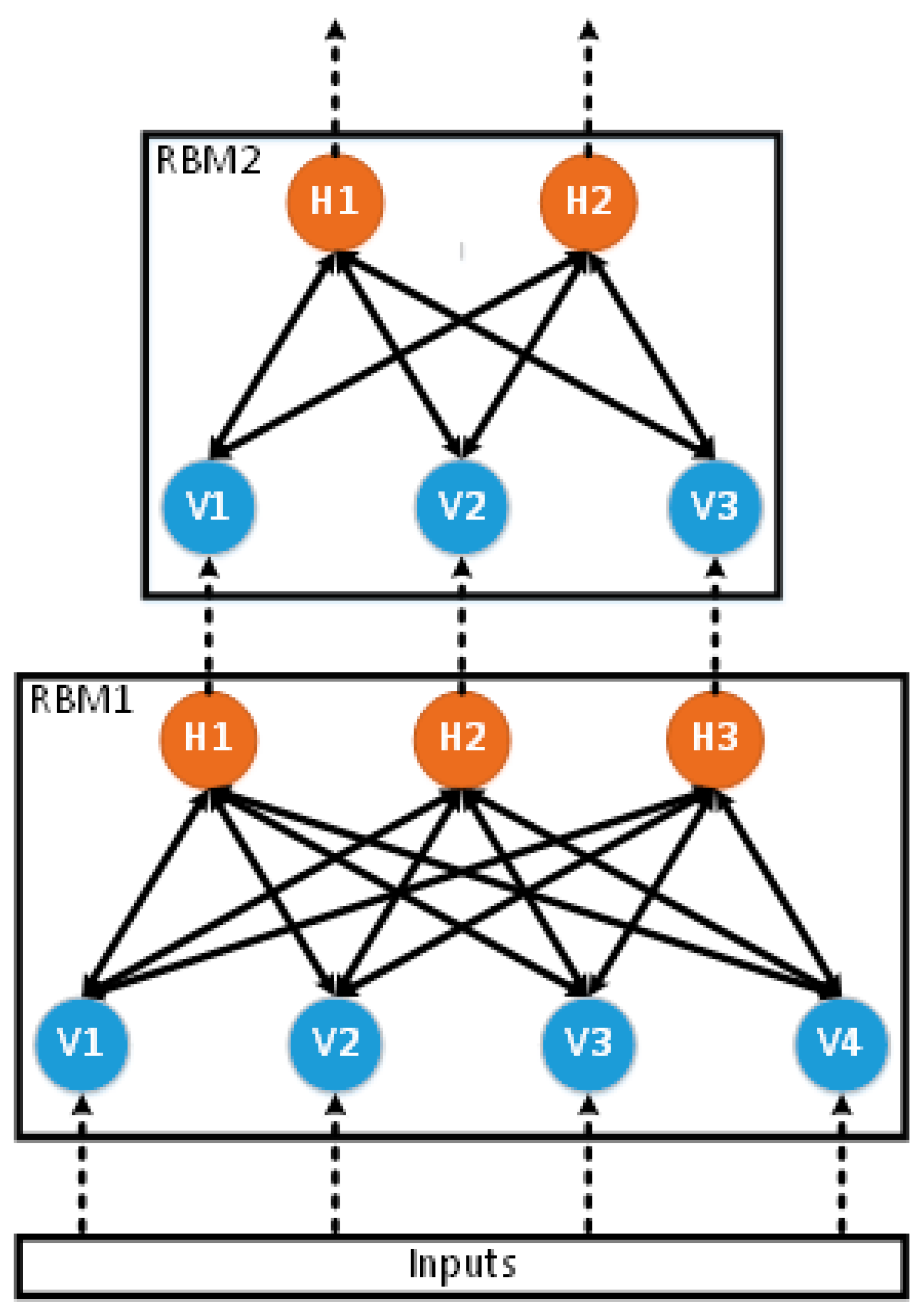
As can be seen in Figure 4, a trained RBM closely resembles a single layer of an ANN. We stack RBMs to form an ANN. First, RBM1 is trained based on our input data using Algorithm 1. Then, the entire input set is fed into the visible layer of a now fixed RBM1, and the outputs at the hidden layer are collected. These outputs are used as the inputs to train RBM2. This process is repeated after RBM2 is fully trained to generate the inputs for RBM3, and so on, as shown in Figure 5. This training is unsupervised, meaning that no target outputs are given to the model. It has information about the inputs and how they are related to one another, but the network is not able to solve any real problem yet.
The next step is training a DNN. Backpropagation is used to train the neural network to solve a particular problem. Since our problem is short-term load forecasting, natural gas load values are used as target outputs, and a set of features such as temperature, wind speed, day of the week, and previous loads are used as the inputs. After the backpropagation training, the DNN functions identically to a large ANN.
5. Data
One common problem with training any type of neural network is that there is always some amount of randomness in the results [27]. This means that it is difficult to know whether a single trained model is performing well because the model parameters are good or because of randomness. Hanson and Salamon mitigated this problem using cross validation and an ensemble of similar neural networks [27]. They trained many models on the different parts of the same set of data so that they could test their models on multiple parts of the data.
This paper mitigates this problem by using data sets from 62 operating areas from local distribution companies around the United States. These operating areas come from many different geographical regions including the Southwest, the Midwest, West Coast, Northeast, and Southeast and thus represent a variety of climates. The data sets also include a variety of urban, suburban and rural areas. This diverse data set allows for broader conclusions to be made about the performance of the forecasting techniques.
For each of the 62 operating areas, several models are trained using at least 10 years of data for training and 1 year for testing. The inputs to these models are those discussed in Section 2. The natural gas flow is normalized using the method proposed by Brown et al. [28]. All the weather inputs in this experiment are observed weather as opposed to forecasted weather for the sake of simplicity.
6. Methods
This section discusses the models at the core of this paper. Four models are compared: a linear regression (LR) model [5], an ANN trained as described in Reference [26], and two DNNs trained as described in Section 3. The first DNN is a shallow neural network with the same size and shape as the ANN. The other DNN is much larger.
The ANN has two hidden layers of 12 and four nodes each and is trained using a Kalman filter-based algorithm [29]. The first DNN has the same architecture as the ANN but is pretrained using contrastive divergence. The purpose of using this model is to determine if the contrastive divergence algorithm can outperform the Kalman filter-based algorithm on these 62 data sets when all other variables are equal. Each RBM is trained for 1000 epochs, and 20 epochs of backpropagation are performed. Despite its small size, the contrastive divergence trained neural network is referred to as a DNN to simplify notation.
In addition to these models, which represent the state-of-the-art in short-term load forecasting of natural gas, a large DNN with hidden layers of 60, 60, 60, and 12 neurons, respectively, is studied. The purpose of this model is to show how much improvement can be made by using increasingly complex neural network architectures. All forecasting methods are provided with the same inputs to ensure a fair comparison.
7. Results
To evaluate the performance of the respective models, we considered several metrics to evaluate the performance of each model. The first of these is the root mean squared error:
for a testing vector of length N, actual demand s, and forecasted demand ŝ. RMSE is a powerful metric for short-term load forecasting of natural gas because it naturally places more value on the days with higher loads. These days are important, as they are when natural gas is the most expensive, which means that purchasing gas on the spot market or having bought too much gas can be costly. Unfortunately, RMSE is magnitude dependent, meaning that larger systems have larger RMSE if the percent error is constant, which makes it a poor metric for comparing the performance of a model across different systems.
Another common metric for evaluating forecasts is mean absolute percent error,
Unlike RMSE, MAPE is unitless and not dependent on the magnitude of the system. This means that it is more useful for comparing the performance of a method between operating areas. It does, however, put some emphasis on the lowest flow days, which, on top of being the least important days to forecast correctly, are often the easiest days to forecast. As such, MAPE is not the best metric for looking at the performance of the model across all the days in a year, but can be used to describe the performance on a subset of similar days.
The error metric used in this paper is weighted MAPE:
This error metric does not emphasize the low flow and less important days while being unitless and independent of the magnitude of the system. This means that it is the most effective error metric for comparing the performance of our methods over the course of a full year.
The mean and standard deviation of the performance of each model over the 62 data sets are shown in Table 1. As expected, the DNN has a lower mean WMAPE than the linear regression and ANN forecasters, meaning that generally, the DNN performs better than the simpler models. Additionally, the large DNN marginally outperforms the small DNN in terms of WMAPE. Both results are shown to be statistically significant later in this section. In addition to the mean, the standard deviation of the performances of the two DNN architectures are smaller than that of the LR and ANN. This is an important result because it points to a more consistent performance across different areas as well as better performance overall.
Simply stating the mean performance does not tell us much without looking at the differences in performance for each of the 62 areas individually, which is shown succinctly in Figure 6 and Figure 7. Figure 6a,b and Figure 7 are histograms of the difference in performance on all 62 areas of two forecasting methods. By presenting the results this way, we can visualize the general difference in performance for each of the 62 operating areas. Additionally, t-tests can be performed on the histograms to determine the statistical significance of the difference. Right-tailed t-tests were performed on the distributions in Figure 6a,b. The resulting p-values are 1.2 × 10⁻⁷ and 6.4 × 10⁻⁴, respectively, meaning that the DNN performed better, in general, than the ANN or LR, and that the difference in performance is statistically significant in both cases.
It is also interesting to consider that in some areas, the LR and ANN forecasters perform better than the DNN. This implies that in some cases, the simpler model is the better forecaster. It is also important to point out that of the 13 areas where the LR outperforms the DNN, only two have LR WMAPEs greater than 5.5, which means that the simple LR models are performing very well when compared to industry standards for short-term load forecasting of natural gas on those areas.
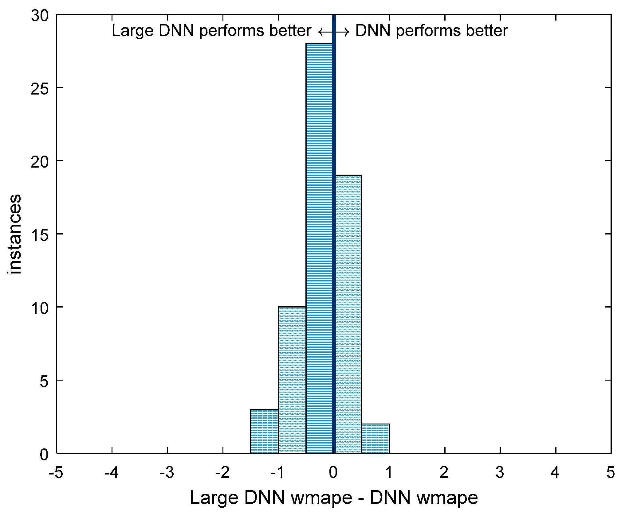
Figure 7 compares the performance of the two DNNs. As with the two distributions in Figure 6, a left-tailed t-test was performed on the histogram in Figure 7 resulting in a p-value of 9.8 × 10⁻⁵. This means that the Large DNN offers a statistically significant better performance over the 62 areas than the small DNN. However, much like in the comparison between the DNN and other models, the small DNN performs better in some areas, which supports the earlier claim that complex models do not necessarily outperform simpler ones.
8. Conclusions
We conclude that DNNs can be better short-term load forecasters than LR and ANNs. On average, over the 62 operating areas examined, a DNN outperformed an otherwise identical ANN at short-term load forecasting of natural gas, and a larger DNN offered even greater performance. However, these improvements to the performance are not present for all 62 operating areas. For some, even the much simpler linear regression model is shown to perform better than the DNN. For this reason, it is concluded that, although the DNN is a powerful option that in general will perform better than simpler forecasting techniques, it may not do so for every operating area. Therefore, DNNs can be used as a tool in short-term load forecasting of natural gas, but multiple other forecasting methods should be considered as well.
Author Contributions
G.D.M. and R.J.P. conceived and designed the experiments G.D.M. performed the experiments; G.D.M. and R.J.P. analyzed the data; R.H.B. contributed reagents/materials/analysis tools; G.D.M. and R.J.P. wrote the paper.
Funding
This research received no external funding.
Acknowledgments
The GasDay lab at Marquette University provided funding and data for this work.
Conflicts of Interest
The authors declare no conflicts of interest.
Nomenclature
| b | bias term of a neural network node |
| c | the bias term of a restricted Boltzmann machine (RBM) |
| CDD | cooling degree days |
| DPT | dew point |
| Dth | dekatherm |
| h | vector of hidden nodes of a RBM |
| HDD | heating degree days |
| hj | jth hidden node of a RBM |
| MAPE | mean absolute error |
| o | output of a neural network node |
| RMSE | root mean square error |
| s | natural gas demand |
| T | temperature in degrees Fahrenheit |
| Tref | reference temperature for HDD and CDD |
| v | vector of visible nodes of a RBM |
| vi | ith visible node of a RBM |
| W | weight matrix of a neural network |
| wi | weight of the ith input of a neural network node |
| WMAPE | weighted mean absolute percentage error |
| xi | ith input to the node of a neural network |
References
- Natural Gas Explained. Available online: https://www.eia.gov/energyexplained/index.php?page=natural_gas_home (accessed on 24 July 2018).
- Merkel, G.D.; Povinelli, R.J.; Brown, R.H. Deep neural network regression for short-term load forecasting of natural gas. In Proceedings of the International Symposium on Forecasting, Cairns, Australia, 25–28 June 2015; p. 90. [Google Scholar]
- Asbury, J.G.; Maslowski, C.; Mueller, R.O. Solar Availability for Winter Space Heating: An Analysis of the Calendar Period, 1953–1975; Argonne National Laboratory: Argonne, IL, USA, 1979.
- Dahl, M.; Brun, A.; Kirsebom, O.; Andresen, G. Improving short-term heat load forecasts with calendar and holiday data. Energies 2018, 11, 1678. [Google Scholar] [CrossRef]
- Vitullo, S.R.; Brown, R.H.; Corliss, G.F.; Marx, B.M. Mathematical models for natural gas forecasting. Can. Appl. Math. Q. 2009, 17, 807–827. [Google Scholar]
- Ishola, B. Improving Gas Demand Forecast during Extreme Cold Events. Master’s Thesis, Marquette University, Milwaukee, WI, USA, 2016. [Google Scholar]
- Haida, T.; Muto, S. Regression based peak load forecasting using a transformation technique. IEEE Trans. Power Syst. 1994, 9, 1788–1794. [Google Scholar] [CrossRef]
- Hornik, K.; Stinchcombe, M.; White, H. Multilayer feedforward networks are universal approximators. Neural Netw. 1989, 2, 359–366. [Google Scholar] [CrossRef]
- Park, D.C.; El-Sharkawi, M.A.; Marks, R.J.; Atlas, L.E.; Damborg, M.J. Electric load forecasting using an artificial neural network. IEEE Trans. Power Syst. 1991, 6, 442–449. [Google Scholar] [CrossRef] [Green Version]
- Längkvist, M.; Karlsson, L.; Loutfi, A. A review of unsupervised feature learning for time series modeling. Pattern Recognit. Lett. 2014, 42, 11–24. [Google Scholar] [CrossRef]
- Szegedy, C.; Liu, W.; Jia, Y.; Sermanet, P.; Reed, S.; Anguelov, D.; Erhan, D.; Vanhoucke, V.; Rabinovich, A. Going deeper with convolutions. In Proceedings of the 2015 IEEE Conference on Computer Vision and Pattern Recognition (CVPR), Boston, MA, USA, 7–12 June 2015; pp. 1–9. [Google Scholar]
- Hinton, G.E.; Hinton, G.E.; Osindero, S.; Osindero, S.; Teh, Y.W.; Teh, Y.W. A fast learning algorithm for deep belief nets. Neural Comput. 2006, 18, 1527–1554. [Google Scholar] [CrossRef] [PubMed]
- Qiu, X.; Zhang, L.; Ren, Y.; Suganthan, P.N.; Amaratunga, G. Ensemble deep learning for regression and time series forecasting. In Proceedings of the 2014 IEEE Symposium on Computational Intelligence in Ensemble Learning, Orlando, FL, USA, 9–12 December 2014; pp. 1–6. [Google Scholar] [CrossRef]
- Busseti, E.; Osband, I.; Wong, S. Deep Learning for Time Series Modeling; Stanford University: Stanford, CA, USA, 2012. [Google Scholar]
- Dalto, M.; Matusko, J.; Vasak, M. Deep neural networks for time series prediction with applications in ultra-short-term wind forecasting. In Proceedings of the IEEE International Conference on Industrial Technology (ICIT), Seville, Spain, 17–19 March 2015; pp. 1657–1663. [Google Scholar]
- Kuremoto, T.; Kimura, S.; Kobayashi, K.; Obayashi, M. Time series forecasting using a deep belief network with restricted Boltzmann machines. Neurocomputing 2014, 137, 47–56. [Google Scholar] [CrossRef]
- Glorot, X.; Bengio, Y. Understanding the difficulty of training deep feedforward neural networks. In Proceedings of the Thirteenth International Conference on Artificial Intelligence and Statistics, Sardinia, Italy, 13–15 May 2010; Teh, Y.W., Titterington, M., Eds.; PMLR: London, UK, 2010; pp. 249–256. [Google Scholar]
- Kennedy, J.; Eberhart, R. Particle swarm optimization. In Proceedings of the IEEE International Conference on Neural Networks, Perth, Australia, 27 November–1 December 1995; Volume 4, pp. 1942–1948. [Google Scholar]
- Ryu, S.; Noh, J.; Kim, H. Deep neural network based demand side short term load forecasting. Energies 2017, 10, 3. [Google Scholar] [CrossRef]
- Kuo, P.-H.; Huang, C.-J. A high precision artificial neural networks model for short-term energy load forecasting. Energies 2018, 11, 213. [Google Scholar] [CrossRef]
- Li, C.; Ding, Z.; Yi, J.; Lv, Y.; Zhang, G. Deep belief network based hybrid model for building energy consumption prediction. Energies 2018, 11, 242. [Google Scholar] [CrossRef]
- Chen, K.; Chen, K.; Wang, Q.; He, Z.; Hu, J.; He, J. Short-term load forecasting with deep residual networks. IEEE Trans. Smart Grid 2018. [Google Scholar] [CrossRef]
- Hosein, S.; Hosein, P. Load forecasting using deep neural networks. In Proceedings of the IEEE Power & Energy Society Innovative Smart Grid Technologies Conference (ISGT), Washington, DC, USA, 23–26 April 2017; pp. 1–5. [Google Scholar]
- Lin, C.-T.; Lee, C.S.G. Neural Fuzzy Systems—A Neuro-Fuzzy Synergism to Intelligent Systems; Prentice-Hall: Upper Saddle River, NJ, USA, 1996. [Google Scholar]
- Bengio, Y. Learning deep architectures for AI. Found. Trends Mach. Learn. 2009, 2, 1–127. [Google Scholar] [CrossRef]
- Hinton, G. A practical guide to training restricted Boltzmann machines. In Neural Networks: Tricks of the Trade; Springer: Berlin/Heidelberg, Germany, 2012. [Google Scholar]
- Hansen, L.K.; Salamon, P. Neural network ensembles. IEEE Trans. Pattern Anal. Mach. Intell. 1990, 12, 993–1001. [Google Scholar] [CrossRef] [Green Version]
- Brown, R.H.; Vitullo, S.R.; Corliss, G.F.; Adya, M.; Kaefer, P.E.; Povinelli, R.J. Detrending daily natural gas consumption series to improve short-term forecasts. In Proceedings of the IEEE Power and Energy Society General Meeting, Denver, CO, USA, 26–30 July 2015. [Google Scholar]
- Ruchti, T.L.; Brown, R.H.; Garside, J.J. Kalman based artificial neural network training algorithms for nonlinear system identification. In Proceedings of the IEEE International Symposium on Intelligent Control, Chicago, IL, USA, 25–27 August 1993; pp. 582–587. [Google Scholar]
Figure 1.
Weighted combination of several midwestern U.S. operating areas, including Illinois, Michigan, and Wisconsin. Authors obtained data directly from local distribution companies. The data is from 1 January 2003 to 19 March 2018.
Figure 1.
Weighted combination of several midwestern U.S. operating areas, including Illinois, Michigan, and Wisconsin. Authors obtained data directly from local distribution companies. The data is from 1 January 2003 to 19 March 2018.
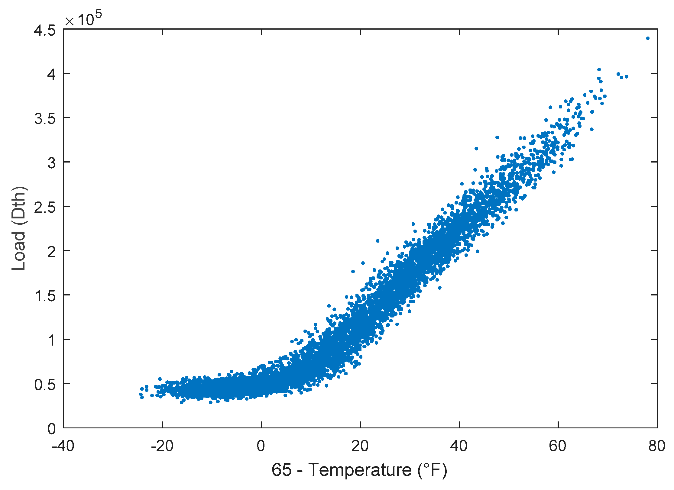
Figure 2.
The same data as in Figure 1 colored by day of the week.
Figure 2.
The same data as in Figure 1 colored by day of the week.

Figure 3.
A feedforward ANN with four visible nodes, three nodes in the first hidden layer, two nodes in the second hidden layer, and a single node in the output layer.
Figure 3.
A feedforward ANN with four visible nodes, three nodes in the first hidden layer, two nodes in the second hidden layer, and a single node in the output layer.

Figure 4.
A restricted Boltzmann machine with four visible units and three hidden units. Note the similarity with a single layer of a neural network.
Figure 4.
A restricted Boltzmann machine with four visible units and three hidden units. Note the similarity with a single layer of a neural network.

Figure 5.
Graphical representation of how RBMs are trained and stacked to function as an ANN.

Figure 6.
This figure shows two histograms: (a) A comparison of the performance of all 62 models between the DNN and the LR. Instances to the left of the center line are those for which the LR performed better, while those on the right are areas where the DNN performs better. The distance from the center line is the difference in WMAPE. (b) The same as (a) but comparing the ANN to the DNN. One instance (at 10.1) in (b) is cut off to maintain consistent axes.
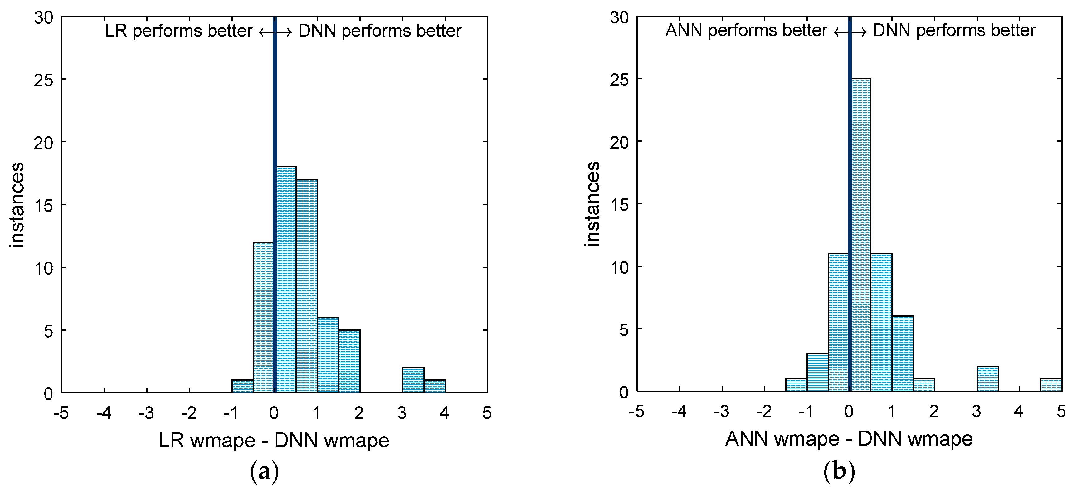
Figure 7.
A comparison of the performance of all 62 models between the DNN and the Large DNN. Instances to the left of the center line are those for which the Large DNN performed better, while those on the right are areas where the DNN performs better. The distance from the center line is the difference in WMAPE.

Table 1.
The mean and standard deviation of the performance of the four models on all 62 areas.
| LR WMAPE | ANN WMAPE | DNN WMAPE | Large DNN WMAPE | |
|---|---|---|---|---|
| Mean | 6.41 | 6.41 | 5.78 | 5.58 |
| Standard Deviation | 2.49 | 2.83 | 2.11 | 2.09 |
© 2018 by the authors. Licensee MDPI, Basel, Switzerland. This article is an open access article distributed under the terms and conditions of the Creative Commons Attribution (CC BY) license (http://creativecommons.org/licenses/by/4.0/).
Share and Cite
MDPI and ACS Style
Merkel, G.D.; Povinelli, R.J.; Brown, R.H. Short-Term Load Forecasting of Natural Gas with Deep Neural Network Regression †. Energies 2018, 11, 2008. https://doi.org/10.3390/en11082008
AMA Style
Merkel GD, Povinelli RJ, Brown RH. Short-Term Load Forecasting of Natural Gas with Deep Neural Network Regression †. Energies. 2018; 11(8):2008. https://doi.org/10.3390/en11082008
Chicago/Turabian StyleMerkel, Gregory D., Richard J. Povinelli, and Ronald H. Brown. 2018. "Short-Term Load Forecasting of Natural Gas with Deep Neural Network Regression †" Energies 11, no. 8: 2008. https://doi.org/10.3390/en11082008
Note that from the first issue of 2016, this journal uses article numbers instead of page numbers. See further details here.