A Multi-Agent System-Based Approach for Optimal Operation of Building Microgrids with Rooftop Greenhouse

Abstract

In this paper, an optimal energy management scheme for building microgrids with rooftop greenhouse is proposed. A building energy management system (BEMS) is utilized for the optimal fulfilment of energy demands in the building and the greenhouse. The exhaust heat generated due to the operation of air conditioners in the building is used for fulfilling the cooling demands of the greenhouse via chillers. In addition to thermal and cooling demands, the four major control parameters (temperature, humidity, light intensity, and CO₂ concentration) are also considered for optimal growth of crops in the greenhouse. A multi-agent system (MAS) is adopted to realize the interaction among several households of the building, the greenhouse, and the BEMS. The MAS comprises of several inner-level, intermediate level, and upper-level agents, which are responsible for their respective tasks. The performance of the proposed optimization strategy is evaluated for two seasons of a year, i.e., summer and winter. Numerical simulations have demonstrated the effectiveness of the proposed operation scheme for optimal operation of building microgrids with rooftop greenhouses.

1. Introduction

The increase in energy demand and greenhouse gas emissions are becoming global issues, and various studies have been conducted to overcome these problems [1,2]. Microgrids are considered a potential solution to these problems due to their ability to sustain the penetration of distributed energy resources, especially renewable energy sources [3,4,5,6]. In [3], the authors have analyzed the benefits of microgrids, i.e., reliability improvement, sustaining the penetration of renewable sources, self-healing, active load control, and improved generation efficiencies. In [4], the impact of intelligent demand management to limit the periods of strain on network and electricity markets is analyzed. In [5,6], the role of microgrids in providing higher local reliability during islanding events in comparison with conventional power system is analyzed.

In addition, several studies on microgrids about demand response (DR), auto-configuration, fault analysis, and control are also available in the literature. Optimal operation of microgrids considering DR and auto-configuration function are studied based on multi-agent system (MAS) in [7,8], respectively. In [9], unsymmetrical faults of microgrids are studied based on definite two relationship matrices. In [10], a versatile convex programming for DR optimization via automatic load management is proposed. In [11], stand-alone hybrid microgrids using general regression neural network and radial basis function network-sliding mode methods are studied for extracting the maximum power output for a hybrid power system. An algorithm is developed in [12] for solving the distribution ground faults of microgrids considering the three phase models. In [13], smart houses having photovoltaic arrays, wind turbine, biomass and geothermal energy are reviewed for optimal operation strategies of households. In [14], an energy consumption model of home appliances in a residential microgrid based on set of sequential uninterruptible energy phases is proposed. During transition from grid-connected to islanded mode, a multi-droop control strategy has been developed to mitigate voltage and frequency variations by [15]. A study of a microgrid using a novel voltage controller using the integration of a vanadium redox battery with solar energy is carried out by [16]. In [17], a novel intelligent damping controller to damp power system oscillations is proposed to improve both transient stability and system oscillations.

There are many types of microgrids and building microgrids have attracted the interest of researchers due to higher consumption of energy [18]. Building microgrids are operated by building energy management systems (BEMSs) [19,20,21,22]. Energy cost was reduced through peak load shaving and load shifting after installing smart systems at buildings by [19]. Based on a linear scheduling model, a schedule for half hourly electricity prices from utility grid and peak demand costs is developed by [20]. In [21], an optimal scheduling for building microgrids considering economic constraints based on temperature dependent thermal load modeling was carried out. The power scheduling and bidding strategy for building microgrids is formulated as a stochastic program by [22] via Monte Carlo simulations.

Meanwhile, the development of the agriculture sector is at its beginning stages and various researches are carried out in [23,24,25]. In [23], the authors have proposed a sophisticated information and communication technology (ICT) infrastructure for gathering, storing, analyzing, and exploiting various information in planning and decision making for future farms. In [24,25] a cloud-based platform is studied for combining agriculture technology with ICT. Intelligent greenhouses are considered an advanced form of conventional greenhouse [26]. Intelligent greenhouses are composed of various sensors and automated management facilities for maintaining the indoor environment. In order to optimize the growth of the crops in greenhouses, four control parameters (i.e., temperature, humidity, CO₂ concentration, and light intensity) must be controlled. Various studies are available in the literature for controlling the internal environment of greenhouses [27,28,29,30]. In [27], study of two fuzzy logic controllers that are comprised of fuzzy proportional and proportional-derivative control using desired climatic set points is carried out. A general framework for a robust adaptive neural network-based feedback linearization controller design for the indoor environment of a greenhouse is studied by [28]. In [29], the use of ‘‘double thermal screen’’ and ‘‘double glazing’’ for assessing energy management of greenhouses are analyzed. The concept of energy management for a closed greenhouse integrated with a thermal energy storage system (TESS) is presented by [30].

Intelligent greenhouses can be integrated into buildings to receive benefit from the advancements in intelligent greenhouses and BEMS technologies, i.e., rooftop greenhouses. A rooftop greenhouse has the potential to create a new agricultural space in the cities using the rooftop, which is otherwise an unproductive space. In addition, by integrating food production into buildings, the self-sufficiency of cities can be increased and transportation requirements and environmental impacts can be reduced [31,32,33,34]. Therefore recently, various research has been performed on the applicability of rooftop greenhouses [35,36,37,38,39,40].

In [35], a residential building with rooftop greenhouse is analyzed for quantifying the environmental impacts and energy requirements. The techno-economic and environmental impacts of integrating rooftop greenhouses in buildings are analyzed by [36,37,38,39]. In [36], the effect on the indoor temperature of the last floor apartments is analyzed by installing greenhouse on the rooftop. The analysis of rooftop greenhouse for controlling energy and emissions flow is carried out via the integration of energy, water, and CO₂ flows. The mutual exchange between greenhouse and building is proposed to reduce the consumption of energy by [37]. The reduction of the carbon footprint of horticultural products produced in urban rooftop greenhouses is observed in these studies. The suitability of the hot air accumulated in the rooftop greenhouse for recirculation to heat the building is evaluated by [38]. In [39], the feasibility of implementation of rooftop greenhouses in non-residential urban areas is analyzed. However, most of the research mentioned in the previous paragraphs are conducted in terms of agricultural engineering and the feasibility of a rooftop greenhouse is not analyzed. Studies on the optimal energy management of buildings with rooftop greenhouses are limited and are more challenging due to the mutual coupling of energies. The concept of a smart rooftop greenhouse, which considers automation and energy efficiency by combining smart grids, is the advanced form of a rooftop greenhouse [40].

In smart rooftop greenhouses, a communication infrastructure is required to interact between the building and the greenhouse. All the components of the greenhouse need to interact with the BEMS to update their status and to receive commands. Similarly, buildings generally have several households. All the households send their information to BEMS and BEMS makes optimal schedules based on the provided information. Due to the widespread use of MAS for optimization of BEMS [41,42,43,44], a MAS can be utilized to realize the communication between BEMS and individual households. In [41], a MAS for microgrids is developed considering the function of agents, interactions among agents, and an effective agent protocol. Utilizing a semi-centralized decision method using MASs for various energy zones (electrical, heating, and cooling) to improve energy efficiency and reduce energy costs is studied by [42]. In [43,44], MASs are developed for the optimal operation of buildings considering the indoor environment and occupants’ comfort.

It can be observed from the literature survey that various studies are available on the internal environment control of greenhouses and rooftop greenhouses. However, most of the research is mainly focused on internal climate control only without considering the energy costs [27,28,29,30]. This may result in a higher operation cost due to the in-optimal utilization of resources. Similarly, studies on the integrated optimal operation of building and rooftop greenhouses are also limited. The integrated optimal operation is challenging due to the coupling of energy sources and the interdependence of loads.

In this paper, an optimal operation strategy is proposed for a smart building with a rooftop greenhouse. The households of the building and the greenhouse have both thermal (heating and cooling) and electrical loads. However, the greenhouse has additional constraints for maintaining the indoor environment by controlling the control parameters. Moreover, the waste heat generated by air-conditioners is utilized to fulfil the heat requirements of the greenhouse. A MAS is developed to realize the interaction among different agents of the building microgrid. Each household in the building has several local agents and an intermediate agent. Similarly, the greenhouse also has several local agents and an intermediate agent. The intermediate agents of each household and the greenhouse are responsible for interacting with the BEMS. The performance of the proposed optimal operation strategy for building microgrid with rooftop greenhouse is tested for two seasons of a year, i.e., winter and summer. The operation schedules of the microgrid equipment and attainment of the control parameters are analyzed for both of the seasons.

2. Proposed Building Microgrids with Rooftop Greenhouse

2.1. Building Microgrids Configuration

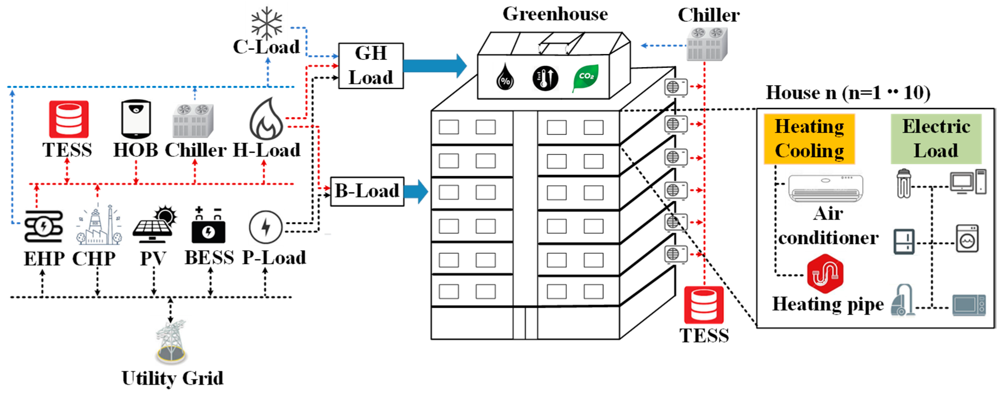
The proposed building microgrid in this study is comprised of a building having n houses and a rooftop greenhouse, i.e., building microgrid with rooftop greenhouse. The configuration of the proposed building microgrid is shown in Figure 1. The building microgrid contains a combined heat and power (CHP) generator, heat only boiler (HOB), chiller, electric heat pump (EHP), photovoltaic (PV) array, TESS, and battery energy storage system (BESS). The equipment specific to the greenhouse is listed in the next section. The building microgrid is connected with the utility grid, thus it can trade power with the utility grid. The cooling demand of houses in the building is fulfilled using the air conditioner units installed in each house. The exhaust heat generated due to the operation of these air conditioners is collected and is used to fulfil the cooling demand of the greenhouse using a chiller. Excess exhaust heat is stored in the TESS unit, as shown in Figure 1. Similarly, the heating demand of the greenhouse is fulfilled using the available heating sources, i.e., CHP, TESS, HOB, and EHP. Finally, the electric demand can be fulfilled either by using the local resources or by trading with the utility grid.

In this study, a building microgrid is considered, which contains n households and a greenhouse on the rooftop of the building. Each household has separate air-conditioner to fulfil its cooling load demands. The heating demands can be fulfilled by using the heat generating equipment of the microgrid via a heat pipe line. Both air conditioner and heat pipe line are used to control the indoor temperature of each household of the microgrid according to its requirements. The residents of each household can specify their departure and arrival times along with their required temperature at arrival time. The BEMS will find an optimal solution to achieve the set target for the specified time in an economic way. Similarly, the users can specify their comfortable range for sleeping time, which will be economically fulfilled by the BEMS. The electric demand can be fulfilled by either using the local power generation or by buying power from the utility grid.

2.2. Greenhouse Configuration and Control Elements

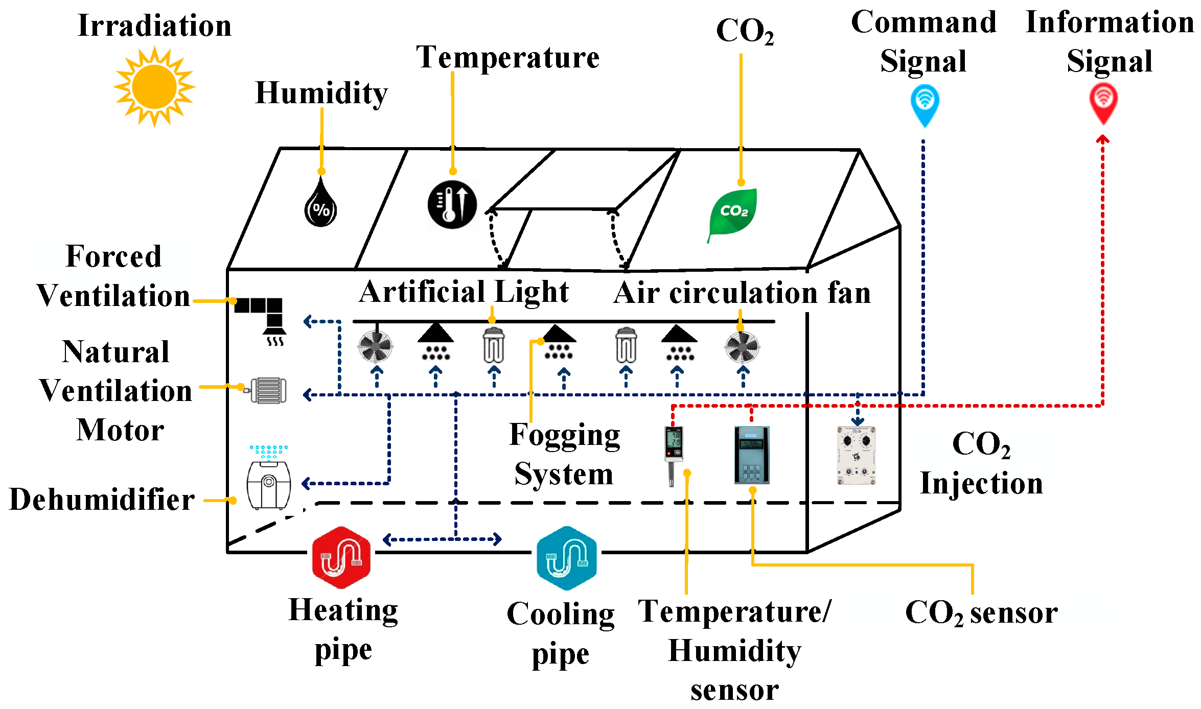
In an intelligent greenhouse, the climate control parameters are automatically controlled to provide optimum conditions for the growth of plants [45]. Climate control is achieved by the automatic control of greenhouse equipment such as ventilation system, automation valves for heating and cooling pipes, fogging system, dehumidifier, artificial light, air circulation fans, and CO₂ injection. Climate control system for greenhouse collects the information from the local sensors and sends suitable control signals to the equipment for their operation. The modeling of the proposed greenhouse for the optimal growth of crops is shown in Figure 2. Each plant has different requirements of control parameters (temperature, humidity, carbon dioxide, and lighting) for its optimal growth [46]. The importance of the four major control factors for optimal growth of plants is described in the following sections.

2.2.1. Indoor Temperature

Indoor temperature is an important factor for crop growth due to its influence on photosynthesis process and respiration [47]. Photosynthesis, being a biochemical reaction, increases with increase in temperature. Similarly, the respiration rate of plants increases with increase in the temperature [48]. However, if temperature is too high or too low, growth of crop is inhibited due to the unsuitable respiration rate and the hindrance of cell activity [49]. Therefore, the indoor temperature of the greenhouse should be controlled within an appropriate range by using the greenhouse equipment.

2.2.2. Humidity

Humidity is the most difficult parameter to control due to its fluctuation with change in air temperature and the transpiration of plants. Inappropriate levels of humidity can adversely affect the plants and cause diseases in the leaves and roots. Additionally, higher humidity halts the transpiration process of plants and lower humidity effects the growth rate. Therefore, humidity should be controlled within an appropriate range by using the greenhouse equipment [50,51].

2.2.3. CO₂ Concentration

Carbon dioxide concentration directly influences the photosynthesis process in crops. The CO₂ compensation point is the point at which the photosynthetic rate and the respiration rate are equal. Therefore, CO₂ concentration should be higher than the CO₂ compensation point for efficient photosynthesis of the plant. The CO₂ saturation point is the point at which the photosynthetic rate does not increase even if the carbon dioxide concentration is increased. Therefore, CO₂ concentration should be controlled between the CO₂ compensation point and the CO₂ saturation point [50,51].

2.2.4. Light Intensity

Light intensity is also an important factor for the optimal growth of crops due to its effect on photosynthesis. If the amount of light is insufficient, the crop growth gets diminished due to the deterioration of photosynthesis. Therefore, light intensity should be maintained above a certain limit.

3. Proposed Multi-Agent System

The proposed optimization algorithm is implemented through a MAS in the building microgrid with rooftop greenhouse. Both the building and the greenhouse have separate task-specific agents and also share some common agents. Details about each of these agents and their respective tasks are explained in the following sections.

3.1. Outer-Level Multi-Agent System

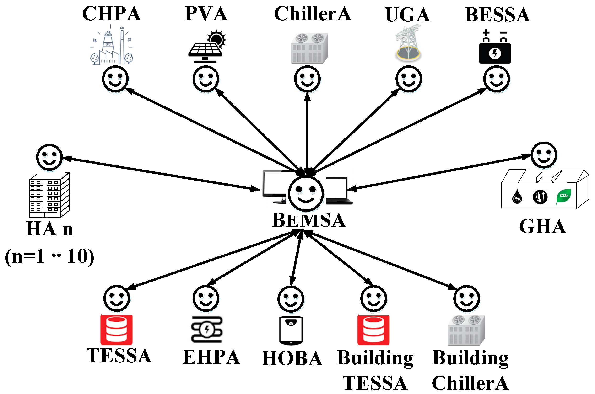
The outer-level MAS consists of the BEMS agent, energy supply facilities, and intermediate agents such as household agents (HAs), and a greenhouse agent (GHA), as shown in Figure 3. The BEMS agent is responsible for the operation of the entire building microgrid with rooftop greenhouse. It receives information from the intermediate agents and makes schedules for the optimal operation of the entire building microgrid. The final schedules are sent to the outer-level agents of the households and the greenhouse. These outer-level agents get information from their respective inner-level agents and inform the schedules received from the BEMS agent to them. The details of inner-level agents along with their respective tasks are explained in the following section.

3.2. Inner-Level Multi-Agent System

3.2.1. Greenhouse Agents

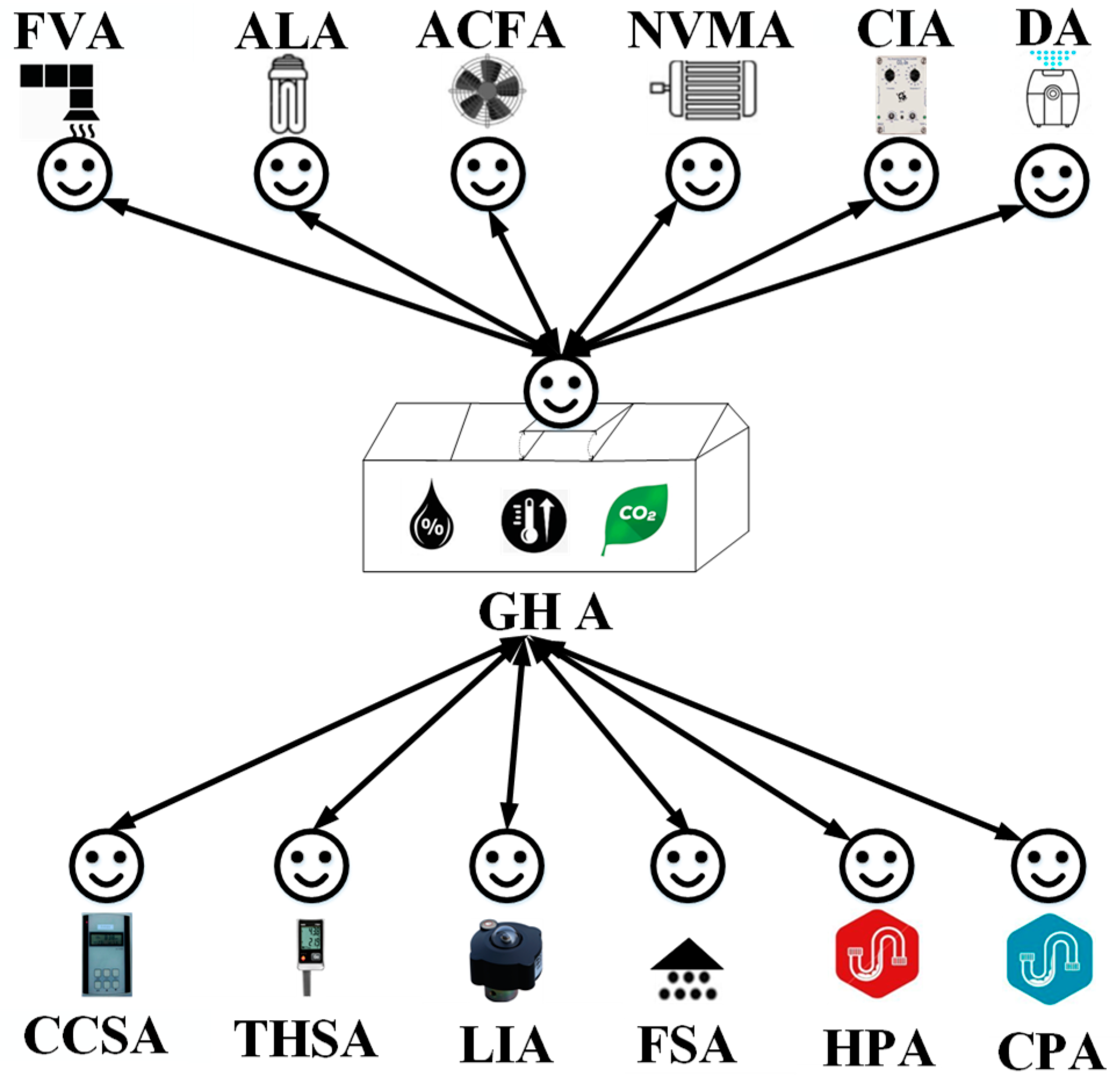
The greenhouse contains active, reactive, and passive agents that are responsible for various tasks. The sensors, such as a CO₂ concentration sensor (CCS), temperature and humidity sensor (THS), and light intensity sensor (LI), are passive agents. These agents periodically send the measured values to the GHA. The agents specific to the equipment of the greenhouse are reactive agents. These agents include a forced ventilation agent (FVA), artificial light agent (ALA), air circulation fans agent (ACFA), natural ventilation motor agent (NVMA), CO₂ injection agent (CIA), dehumidifier agent (DA), fogging system agent (FSA), heating pipe agent (HPA), and cooling pipe agent (CPA) as shown in Figure 4. These agents follow the commands of the GHA and they are reactive agents. The GHA is an active agent, which monitors the status of reactive agents and uses the information of passive agents to make decisions. These decisions are informed to the BEMS agent for updating and/or re-scheduling the resources.

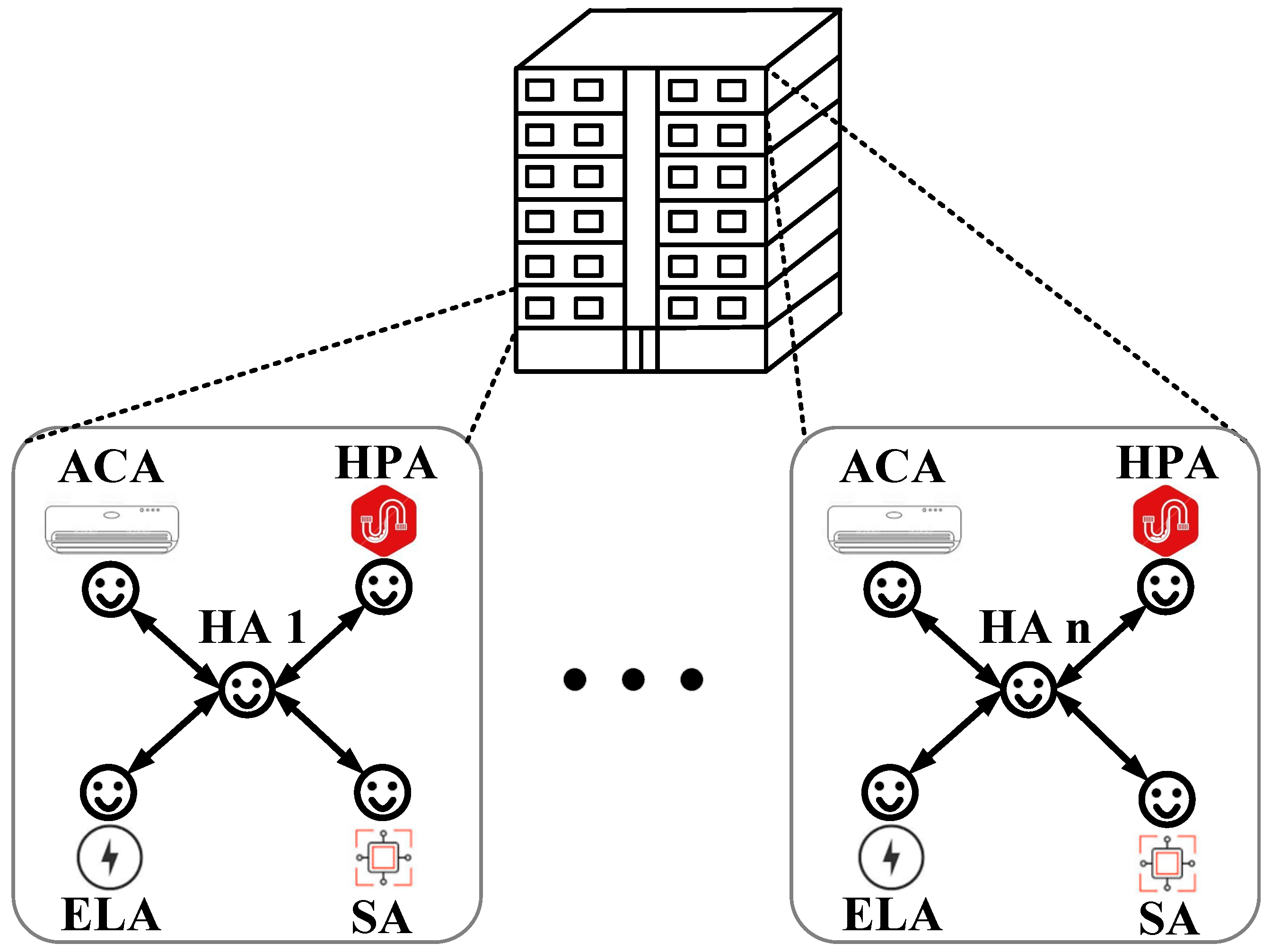
3.2.2. Individual Household Agents

Each household in the building has a set of local agents as shown in Figure 5. Similar to the greenhouse, the agents in an individual household can be categorized as active, passive, and reactive agents. The sensors agents (SA) in each household, which are responsible for sending their measured data periodically to their respective HA are the passive agents. The equipment-specific agents (i.e., air-conditioner agent (ACA), HPA, and electric load agent (ELA)) are reactive agents. The HA in each household is an active agent that uses the information of its inner-level agents to make decisions and communicates with the BEMS agents. Residents of each household can specify their desired temperature setting values and their arrival and departure times to their respective HA. The HA will communicate this information with the BEMS agent and get optimal schedules for the equipment to fulfil the user demands.

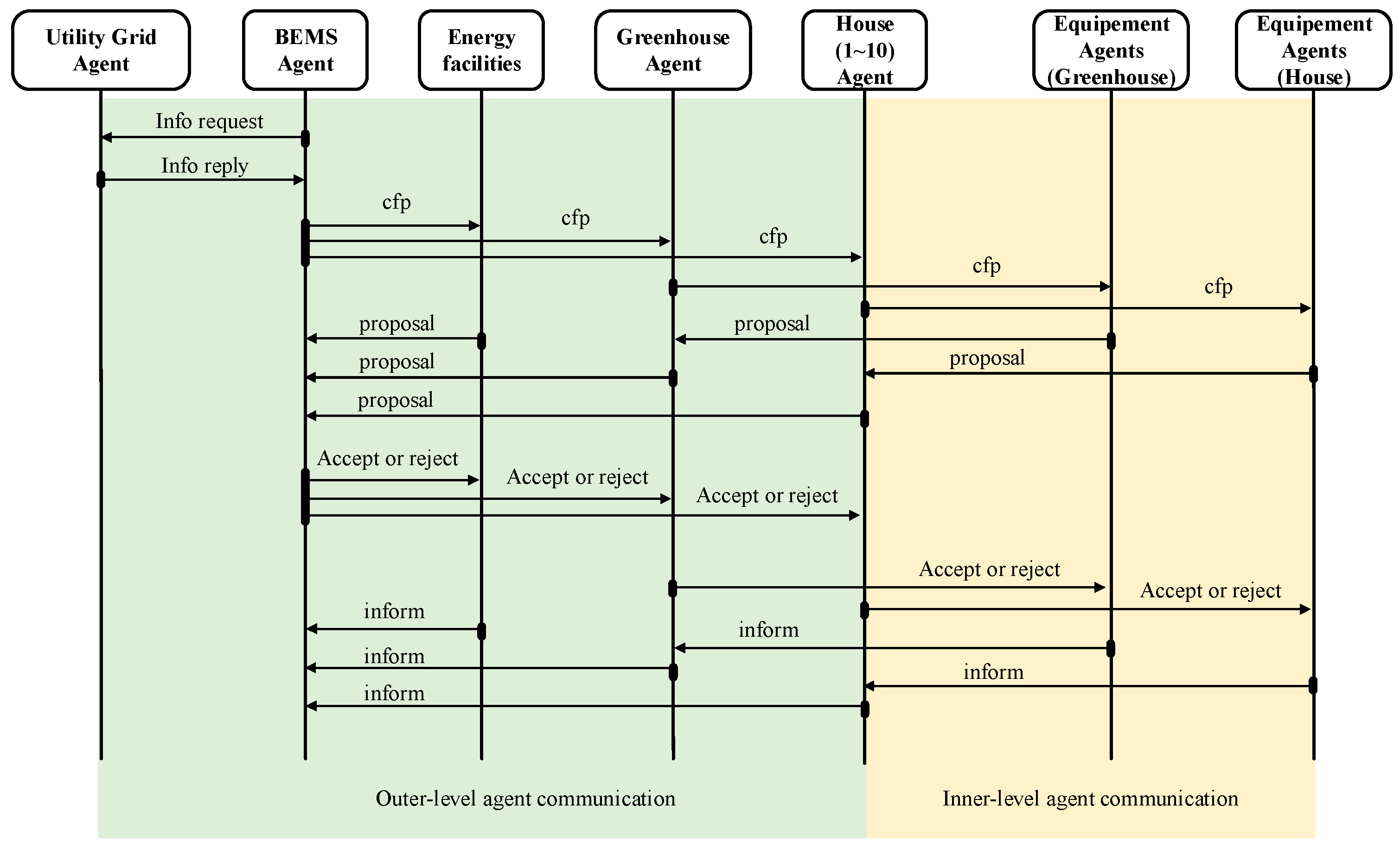
3.3. Communication among Different Agents

In this study, communication among the agents is realized through agent communication language (ACL) messages by using modified contract net protocol (MCNP) [52]. The communication between different agents in the proposed scheme is shown in Figure 6. Firstly, the BEMS agent sends message to the utility grid agent for inquiring the market price signals. The utility grid agent sends the day-ahead market price for each hour of the day to the BEMS agent. Then, the BEMS sends the market price information to the registered outer-level agents along with call for proposal (cfp) messages. The outer-level agents having inner-level agents (GHA and HAs) send cfp messages to their respective registered inner-level agents. After receiving the required information such as generation cost, capacity, and operation status from inner-level agents, outer level agents decide their participation in the operation. The outer-level agents send the collective information to the BEMS agent or send a refusal message. Similarly, each individual inner-level agent can send its refusal messages, if it is not willing to participate in the operation process. After receiving the information from all agents, the BEMS performs the optimization and sends the acceptance or rejection messages about proposals to each agent. In case of acceptance, outer level agents send the schedules received from the BEMS to the registered inner-level agents. In this way, one round of optimization is completed for the proposed building microgrid with rooftop greenhouse. The detailed process for communication among different outer-level agents and the BEMS is shown in Algorithm 1. Algorithm 2 shows the detailed process for communication among outer-level agents and their respective registered inner-level agents.

Algorithm 1. Communication among BEMS agent and outer level agents using modified contract net protocol (MCNP).

Algorithm 2. Communication among intermediate agents and local agents using MCNP.

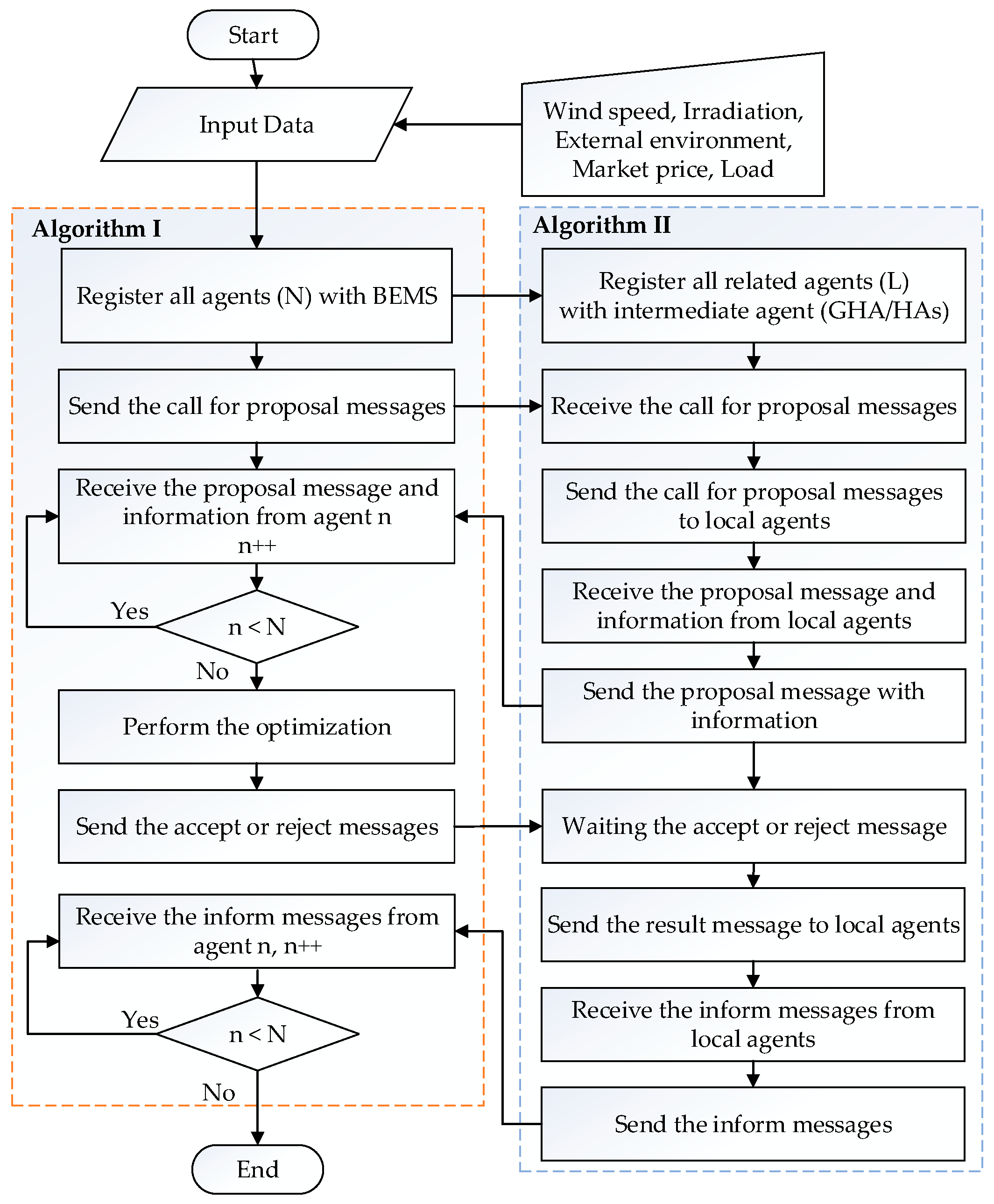
3.4. Flowchart for Building Microgrid with Rooftop Greenhouse Using Multi-Agent System

The flowchart for building a microgrid with rooftop greenhouse using a MAS is shown in Figure 7. The BEMS agent receives the information, such as buying and selling price signals from the utility grid, external environment parameters, and load profiles. BEMS communicates with other agents for getting their information following Algorithms 1 and 2. After receiving all information, BEMS performs optimization and informs the optimal schedules to other agents. The output of each energy supply equipment is decided for minimizing the operation cost of the microgrid network. The amount of trading power with the utility grid is decided to maximize the profit of the microgrid.

4. Estimation of Greenhouse and Building Control Parameters

The estimation methods for the four major control parameters of greenhouse, considered in this study, are described in the following sections.

4.1. Indoor Temperature of Greenhouse and Building

The indoor temperature of greenhouse can be calculated using Equation (1) [53]. Temperature of greenhouse at time t (${\theta }_t^{gh}$), in °C, is a function of greenhouse temperature at previous time interval t − 1 (${\theta }_{t-1}^{gh}$) and temperature change at current time interval. Temperature change at current time interval is function of following parameters.

• $j_t^{sr}$: Heat absorbed from solar radiations (kJ/h)
• $j_t^{gh\_htp}$: Heat exchanged through heating pipe (kJ/h)
• $j_t^{gh\_chlp}$: Heat exchanged through cooling pipe (kJ/h)
• $j_t^{gh\_wall}$: Heat exchanged through wall of the greenhouse (kJ/h)
• $j_t^{nv}$: Heat exchanged due to natural ventilation (kJ/h)
• $j_t^{fv}$: Heat exchanged due to forced ventilation (kJ/h)
• $j_t^{gh\_soil}$: Heat exchanged through soil of the greenhouse (kJ/h)
• $j_t^{li}$: Heat absorbed due to operation of artificial lights (kJ/h)
• $j_t^{c{o}_2}$: Heat absorbed due to operation of CO₂ generator (kJ/h)
• $j_t^{dh}$: Heat absorbed due to operation of dehumidifier (kJ/h)
• $j_t^{ev}$: Heat lost due to operation of fogging system (kJ/h)

In Equation (1), $S{H}^a$, ${\rho }_a$, and $V^{gh}$ are specific heat of air, air density, and volume of the greenhouse in kJ/(kg K), kg/m³, and m³, respectively.

$${\theta }_t^{gh}={\theta }_{t-1}^{gh}+\frac{1}{S{H}^a\cdot {\rho }_a\cdot V^{gh}}\cdot \left(\begin{array}{l}{j}_t^{sr}+j_t^{gh\_htp}+j_t^{gh\_chlp}+j_t^{gh\_wall}+j_t^{nv}+j_t^{fv}-j_t^{gh\_soil}\\ +j_t^{li}+j_t^{c{o}_2}+j_t^{dh}-j_t^{ev}\end{array}\right)\forall t\in T$$

(1)

Water temperature of pipe (${\theta }_t^{gh\_htp}$, ${\theta }_t^{gh\_chlp}$) effects the performance of the cooling and heating systems. When the pipe valve ($u_t^{gh\_htp}$, $u_t^{gh\_chlp}$) is on, heat is exchanged between the pipe and the greenhouse according to the heat transfer coefficient of the pipe (${\eta }^{gh\_pipe}$) and area of the pipe ($A^{gh\_htp}$, $A^{gh\_chlp}$) in m². Similarly, heat is exchanged between the pipe and the soil according to the heat transfer coefficient of the soil (${\eta }^{gh\_soil}$) due to the temperature difference between them (${\theta }_t^{gh\_htp}-{\theta }_t^{gh\_soil}$). The water temperature of the heating and cooling pipes can be calculated using Equations (2) and (3), respectively. For calculating the water temperature of pipe, specific heat of water ($S{H}^w$) in kJ/(kg K), water density (${\rho }_w$) in kg/m³, and volume of respective pipes ($V^{gh\_htp}$, $V^{gh\_chlp}$) in m³ are used. In Equation (2), $H_t^{gh}$ is the heat load of the greenhouse and $C_t^{Load}$ in Equation (3) is the cooling load of the greenhouse.

$${\theta }_t^{gh\_htp}={\theta }_{t-1}^{gh\_htp}+\frac{1}{F^{htp}}\cdot \left(\begin{array}{l}3600\cdot H_t^{gh}\\ -{\eta }^{gh\_pipe}\cdot A^{gh\_htp}\cdot u_t^{gh\_htp}\cdot ({\theta }_t^{gh\_htp}-{\theta }_t^{gh})\\ -{\eta }^{gh\_soil}\cdot A^{gh\_htp}\cdot u_t^{gh\_htp}\cdot ({\theta }_t^{gh\_htp}-{\theta }_t^{gh\_soil})\end{array}\right)\forall t\in T$$

(2)

$${\theta }_t^{gh\_chlp}={\theta }_{t-1}^{gh\_chlp}+\frac{1}{V^{chlp}}\cdot \left(\begin{array}{l}-3600\cdot C_t^{Load}\\ -{\eta }^{gh\_pipe}\cdot A^{gh\_chlp}\cdot u_t^{gh\_chlp}\cdot ({\theta }_t^{gh\_chlp}-{\theta }_t^{gh})\\ -{\eta }^{gh\_soil}\cdot A^{gh\_chlp}\cdot u_t^{gh\_chlp}\cdot ({\theta }_t^{gh\_chlp}-{\theta }_t^{gh\_soil})\end{array}\right)\forall t\in T$$

(3)

where $F^{htp}=S{H}^w\cdot {\rho }_w\cdot V^{gh\_htp}$, $F^{chlp}=S{H}^w\cdot {\rho }_w\cdot V^{gh\_chlp}$.

The variables $u_t^{gh\_htp},u_t^{gh\_chlp}$ indicate the operation status of heating and cooling pipe valves. Due to the presence of two variables ($u_t^{gh\_htp},{\theta }_t^{gh\_htp}$ and $u_t^{gh\_chlp},{\theta }_t^{gh\_chlp}$), Equations (2) and (3) are nonlinear. These nonlinear equations can be converted to linear counterparts by using reformulation-linearization techniques [54,55].

The indoor temperature of each household in the building can be calculated using Equation (4). Temperature of household at time t (${\theta }_{t,n}^{in}$) is a function of household temperature at the previous time interval t − 1 (${\theta }_{t-1,n}^{in}$) and temperature change at the current time interval. Temperature change at the current time interval is a function of the following parameters:

• $j_{t,n}^{ac}$: Heat absorbed from solar radiations (kJ/h)
• $j_{t,n}^{ho\_htp}$: Heat exchanged through heating pipe (kJ/h)
• $j_{t,n}^{ho\_wall}$: Heat exchanged through wall of each households (kJ/h)

In Equation (4), $V_n^{ho}$ is the volume of each household.

$${\theta }_{t,n}^{ho}={\theta }_{t-1,n}^{ho}+\frac{1}{S{H}^a\cdot {\rho }_a\cdot V_n^{ho}}\cdot \left(j_{t,n}^{ac}+j_{t,n}^{ho\_htp}+j_{t,n}^{ho\_wall}\right)\forall t\in T,\forall n\in N$$

(4)

Water temperature of the heating pipe for each household is similar with Equation (2).

4.2. Humidity Control for Greenhouse

The relative humidity of the greenhouse ($R{H}_t^{gh}$) in % can be computed using partial ($p_t^{gh\_par}$) and saturated vapor pressures ($p_t^{gh\_sat}$) in Pa, as given by Equation (5). The saturated vapor can be computed using nonlinear Equation (6). This nonlinear equation can be transformed into a linear equation using Taylor series [56]. The partial pressure of vapor is a function of the atmospheric pressure ($p^{atm}$) and water contents in the air ($w_t^{gh}$) as shown in Equation (7).

$$R{H}_t^{gh}=\frac{p_t^{gh\_par}}{p_t^{gh\_sat}}\cdot 100\%\forall t\in T$$

(5)

$$p_t^{gh\_sat}=a_1\cdot \left(-a_2+\left(a_3{e}^{\frac{a_4\cdot \left({\theta }_{\min }+{\theta }_{\max }\right)}{2}}\right)\cdot 1+a_4\cdot \left({\theta }_t^{gh}-\frac{\left({\theta }_{\min }+{\theta }_{\max }\right)}{2}\right)\right)\forall t\in T$$

(6)

$$p_t^{gh\_par}=\frac{w_t^{gh}\cdot p^{atm}\cdot {10}^{-3}}{0.6228}\forall t\in T$$

(7)

Water contents in the air (g/kg) at time t is a function of the water contents in the air at a previous time interval t − 1 ($w_{t-1}^{gh}$) and a change in water content at the current time interval t. Water content at t is affected by the transpiration of crops ($w^{tran}$) in g/hm², natural and forced ventilation, fogging system, and dehumidifier. Natural ventilation is effected by the wind speed ($n_t^{ws}$) in m/s, wind entering a ratio through the natural ventilation window (${\eta }^{nv}$), air density (${\rho }_a$), area of natural ventilation window ($A^{nv}$), operation status of natural ventilation ($u_t^{nv}$), and water contents difference in indoor and outdoor ($w_t^{out}-w_t^{gh}$). Forced ventilation is effected by the ventilation speed of fan ($f^{ws}$), air density, area of greenhouse, operation status of forced ventilation ($u_t^{fv}$), and water contents difference in indoor and outdoor. The amount of water content produced by the fogging system depends on its efficiency ($w_{\max }^{fg}/P_{\max }^{fg}$) and amount of power consumed ($P_t^{fg}$). Similarly, the amount of water content absorbed by the dehumidifier depends on its efficiency ($w_{\max }^{dh}/P_{\max }^{dh}$) and amount of power consumed ($P_t^{dh}$).

$$w_t^{gh}=w_{t-1}^{gh}+\frac{1}{{\rho }_a{V}^{gh}}\left(\begin{array}{l}{w}^{tran}\cdot A^{gh}+n_t^{ws}\cdot {\eta }^{nv}\cdot {\rho }_a\cdot A^{nv}\cdot u_t^{nv}\cdot \left(w_t^{out}-w_t^{gh}\right)\\ +f^{ws}\cdot {\rho }_a\cdot A^{gh}\cdot u_t^{fv}\cdot \left(w_t^{out}-w_t^{gh}\right)+P_t^{fg}\cdot \frac{w_{\max }^{fg}}{P_{\max }^{fg}}\cdot A^{gh}-P_t^{dh}\cdot \frac{w_{\max }^{dh}}{P_{\max }^{dh}}\cdot A^{gh}\end{array}\right)\forall t\in T$$

(8)

If the outdoor temperature (${\theta }_t^{out}$) and humidity ($R{H}_t^{out}$) in % are known, the external water contents ($w_t^{out}$) in the air can be calculated using Equations (9)–(11), similar to the internal water contents of the air. The variables $P_t^{out\_sat},P_t^{out\_par}$ indicate the outdoor saturated and partial vapor pressures.

$$p_t^{out\_sat}=a_1\cdot \left(-a_2+a_3{e}^{a_4}\cdot {\theta }_t^{out}\right)\forall t\in T$$

(9)

$$p_t^{out\_par}=\frac{R{H}_t^{out}\cdot p_t^{out\_sat}}{100}\forall t\in T$$

(10)

$$w_t^{out}=\frac{p_t^{out\_par}\cdot 0.6228\cdot 1000}{p^{atm}}\forall t\in T$$

(11)

4.3. CO₂ Concentration Control for Greenhouse

The CO₂ concentration in ppm at time t ($C{O_2}_t^{gh}$) is a function of CO₂ concentration at previous time interval t − 1 ($C{O_2}_{t-1}^{gh}$) and change in CO₂ concentration at the current time interval t (12). CO₂ concentration at t depends on the CO₂ injected by the CO₂ generator ($C{O_2}^{gen}$), natural and forced ventilation, respiration, and photosynthesis. The amount of CO₂ injected by the CO₂ generator depends on its efficiency ($C{O_2}_{\max }^{gen}/P_{\max }^{c{o}_2}$) and amount of power consumed ($P_t^{c{o}_2}$). The CO₂ change due to respiration is calculated using the respiration coefficient of crops ($c^{res}$) in g/m²hK, area of greenhouse, and respiration rate of the crops ($a_5$, $a_6$). The CO₂ change due to photosynthesis is calculated using photosynthesis coefficient of crops ($c^{phot}$) in g/J, total amount of light ($I_t^{total}$) in W/m², and area of the greenhouse.

$$C{O_2}_t^{gh}=C{O_2}_{t-1}^{gh}+\frac{1}{{\rho }_a\cdot V^{gh}}\cdot \left(\begin{array}{l}{P}_t^{c{o}_2}\cdot \frac{C{O_2}_{\max }^{gen}}{P_{\max }^{c{o}_2}}\cdot A^{gh}+f^{ws}\cdot {\rho }_a\cdot A^{gh}\cdot u_t^{fv}\cdot \left(C{O_2}_t^{out}-C{O_2}_t^{gh}\right)\\ +n^{ws}\cdot {\eta }^{nv}\cdot {\rho }_a\cdot A^{nv}\cdot u_t^{nv}\cdot \left(C{O_2}_t^{out}-C{O_2}_t^{gh}\right)+c^{res}\cdot A^{gh}\cdot (a_5+a_6\cdot {\theta }_t^{gh})\\ -3600\cdot c^{phot}\cdot I_t^{total}\cdot A^{gh}\end{array}\right)\forall t\in T$$

(12)

4.4. Light Control for Greenhouse

Light intensity can be calculated using Equation (13). Where, $P_t^{sr}$ is the solar radiations, ${\eta }^{sr}$ is the transmittance of solar light, and $P_{t,i}^{li}$ is the light produced by ith artificial light unit.

$$I_t^{total}=P_t^{sr}\cdot {\eta }^{sr}+{\displaystyle \sum _{i\in I}{P}_{t,i}^{li}}\forall t\in T$$

(13)

5. Problem Formulation

5.1. Objective Function

The objective function aims to minimize the operational costs of the building microgrid. The first term of the objective function (14) shows the generation cost of CHP ($C_i^{CHP}$). The second and third terms show the buying price ($P{R}_t^{Buy}$) and selling price ($P{R}_t^{Sell}$) for trading electricity with the utility grid. The fourth and fifth terms show the operation cost of greenhouse chiller ($C^{Chl}$) and chiller on the building ($C^{Chl\_B}$), respectively. The amount of cooling energy can be computed using the amount of heat used and the energy efficiency ratings of chillers. The last term of (14) shows the operation cost of HOB ($C^{HOB}$).

$$\min {\displaystyle \sum _{t\in T}\left(\begin{array}{l}{\displaystyle \sum _{i\in I}{P}_{t,i}^{CHP}\cdot C_i^{CHP}}+P_t^{Buy}\cdot P{R}_t^{Buy}-P_t^{Sell}\cdot P{R}^{Sell}+C{O}_t^{Chl}\cdot C^{Chl}\\ +C{O}_t^{Chl\_B}\cdot C^{Chl\_B}+H_t^{HOB}\cdot C^{HOB}\end{array}\right)}$$

(14)

where $C{O}_t^{Chl\_B}=H_t^{Chl\_B}\cdot {\eta }^{Chl\_B}$.

5.2. Energy Balancing Constraints

5.2.1. Power Balance

Power generated by CHP ($P_{t,i}^{CHP}$), PV ($P_t^{PV}$), bought from the utility grid ($P_t^{Buy}$), and discharged from BESS ($P_t^{B-}$) should be equal to the total load ($P_t^{TotalLoad}$), power sold to the utility grid ($P_t^{Sell}$), and charged amount to BESS ($P_t^{B+}$) at interval t.

$${\displaystyle \sum _{i\in I}{P}_{t,i}^{CHP}}+P_t^{Buy}+P_t^{PV}+P_t^{B-}=P_t^{TotalPLoad}+P_t^{Sell}+P_t^{B+}\forall t\in T$$

(15)

Total electric load is the sum of the greenhouse load ($P_t^{GLoad}$), building load ($P_t^{BLoad}$), and power consumed by EHP ($P_t^{EHP}$) for generating cooling energy. The electric load of the greenhouse comprises of heating and cooling pipe valves ($P_{\max }^{gh\_htv}\cdot u_t^{gh\_htv}$, $P_{\max }^{gh\_chlv}\cdot u_t^{gh\_chlv}$), air circulation fans ($P_t^{acc}$), natural ($P^{nv}$) and forced ventilation systems ($P^{fv}$), fogging system ($P_t^{fg}$), dehumidifier ($P_t^{dh}$), CO₂ injection ($P_t^{c{o}_2}$) and artificial lights ($P_{t,l}^{li}$). The electric load of the building is composed of heating pipe valve ($P^{B\_htv}\cdot u_{t,n}^{B\_htv}$), air conditioner ($P_{t,n}^{ac}$), and other electric loads in each household n ($P_{t,n}^{ELoad}$). The power consumed by EHP ($P_t^{EHP}$) is the sum of power used for converting heating energy ($P_t^{EHP\_ht}$) and cooling energy ($P_t^{EHP\_cool}$). However, EHP cannot generate heating and cooling energy simultaneously.

$$P_t^{TotalLoad}=P_t^{GLoad}+P_t^{BLoad}+P_t^{EHP}\forall t\in T$$

(16)

where:

$$\begin{gathered} \begin{array}{cc}\hfill P_t^{GLoad}=& P_{\max }^{gh\_htv}\cdot u_t^{gh\_htv}+P_{\max }^{gh\_chlv}\cdot u_t^{gh\_chlv}+P^{acc}\cdot u_t^{acc}+P^{fv}\cdot u_t^{fv}+P^{nv}\cdot u_t^{nv}\hfill \\ & +P_t^{dh}+P_t^{fg}+P_t^{c{o}_2}+{\displaystyle \sum _{l\in L}{P}_{t,l}^{li}\cdot A^{gh}}\hfill \end{array} \\ \begin{array}{cc}\hfill P_t^{BLoad}& ={\displaystyle \sum _{n\in N}(P^{B\_htv}\cdot u_{t,n}^{B\_htv}+P_{t,n}^{ac}+P_{t,n}^{ELoad}})\hfill \\ \hfill P_t^{EHP}& =P_t^{EHP\_ht}+P_t^{EHP\_cool}\hfill \end{array} \end{gathered}$$

5.2.2. Heat Energy Balance

Equation (17) shows the heat balance of the rooftop greenhouse building microgrid. It shows that heat generated by CHP ($H_{t,i}^{CHP}$), HOB ($H_t^{HOB}$), EHP ($H_t^{EHP}$), and discharged amount from TESS ($H_t^{T-}$) should be equal or greater than the heat load ($H_t^{Load}$), heat used by chiller ($H_t^{chl}$), and amount of heat charged to TESS ($H_t^{T+}$) at interval t. The amount of heat generated by CHP was modeled considering the heat to power ratio of CHP. Heat from EHP was modeled considering the coefficient of performance (COP) of EHP. Heat load is the sum of heat load of greenhouse ($H_t^{gh}$) and heat load of each household in the building ($H_{t,n}^{ho}$).

$${\displaystyle \sum _{i\in I}{H}_{t,i}^{CHP}}+H_t^{HOB}+H_t^{T-}+H_t^{EHP}\ge H_t^{Load}+H_t^{chl}+H_t^{T+}\forall t\in T$$

(17)

where $H_{t,i}^{CHP}=P_{t,i}^{CHP}\cdot {\eta }_i^{ht}$, $H_t^{EHP}=P_t^{EHP\_ht}\cdot {\eta }^{EHP\_ht}$, $H_t^{Load}=H_t^{gh}+{\displaystyle \sum _{n\in N}{H}_{t,n}^{ho}}$.

Heat energy collected from the exhaust of the air conditioners ($H_{t,n}^{ac}$) can be used by building a chiller ($H_t^{chl\_B}$) or can be stored in building TESS, which can be later used by building a chiller. The amount of exhaust heat generated by the air conditioner was modeled considering the waste heat generation rate and the amount of power consumed by the air conditioner as given by Equation (18).

$${\displaystyle \sum _{r\in R}{H}_{t,r}^{ac}}+H_t^{TB-}\ge H_t^{chl\_B}+H_t^{TB+}\forall t\in T$$

(18)

where $H_{t,n}^{ac}=P_{t,n}^{ac}\cdot {\eta }_n^{ac}$

5.2.3. Cooling Energy Balance

The cooling energy generated by chiller ($C{O}_t^{Chl}$), building chiller ($C{O}_t^{Chl\_B}$), and EHP ($C{O}_t^{EHP}$) should be equal to the cooling load ($C_t^{Load}$) of the greenhouse, as given by (19). The cooling energy generated by EHP can be calculated considering the power consumed by the EHP along with its COP (${\eta }^{EHP\_cool}$). Similarly, the cooling demand of house r can be fulfilled by using its local AC unit(s), as given by Equation (20).

$$C{O}_t^{Chl}+C{O}_t^{Chl\_B}+C{O}_t^{EHP}=C_t^{Load}\forall t\in T$$

(19)

where $C{O}_t^{EHP}=P_t^{EHP\_cool}\cdot {\eta }^{EHP\_cool}$.

$$C_{t,n}^{ac}=P_{t,n}^{ac}\cdot {\eta }_n^{ac}\forall t\in T,n\in N$$

(20)

5.3. Greenhouse Constraints

Temperature constraints are divided into daytime (${\theta }_{\min }^{daytime}$, ${\theta }_{\max }^{daytime}$) and non-day time (${\theta }_{\min }^{normal}$, ${\theta }_{\max }^{normal}$) as shown in Equation (21). An addition bound for average temperature (${\theta }_{\min }^{aver}$, ${\theta }_{\max }^{aver}$) is also considered, as shown in Equation (22). Constraints of water temperatures for the heat pipe (${\theta }_{\min }^{gh\_htp}$, ${\theta }_{\max }^{gh\_htp}$) and cooling pipe (${\theta }_{\min }^{gh\_chlp}$, ${\theta }_{\max }^{gh\_chlp}$) are given by Equation (23). Constraints of water contents in the air of Equations (24) and (25) are modeled using Equations (5)–(7). Therefore, the relative humidity can be controlled within the range ($R{H}_{\min }$, $R{H}_{\max }$) as given by Equation (26). Constraints of CO₂ concentration ($C{O}_{2_{\min }}$, $C{O}_{2_{\max }}$) are given by Equation (27). Constraint of light intensity ($I_{\min }^{total}$) is given by Equation (28). Equations (29)–(32) are constraints of each equipment for controlling the internal environmental of greenhouse, i.e., dehumidifier ($P_{\max }^{dh}$), fogging ($P_{\max }^{fg}$), CO₂ generator ($P_{\max }^{c{o}_2}$), and artificial lights ($P_{\max }^{li}$). Constraints of air circulation fan ($ac{c}_{\min }$) are given by Equations (33) and (34).

$$\{\begin{array}{l}{\theta }_{\min }^{daytime}\le {\theta }_t^{gh}\le {\theta }_{\max }^{daytime}\mathrm{if},10\le t\le 18\\ {\theta }_{\min }^{normal}\le {\theta }_t^{gh}\le {\theta }_{\max }^{normal}\mathrm{else}\end{array}\forall t\in T$$

(21)

$${\theta }_{\min }^{aver}\le {\displaystyle \sum _{t\in T}\frac{{\theta }_t^{gh}}{T}}\le {\theta }_{\max }^{aver}\forall t\in T$$

(22)

$${\theta }_{\min }^{gh\_htp}\le {\theta }_t^{gh\_htp}\le {\theta }_{\max }^{gh\_htp},{\theta }_{\min }^{gh\_chlp}\le {\theta }_t^{gh\_chlp}\le {\theta }_{\max }^{gh\_chlp}\forall t\in T$$

(23)

$$w_t^{in}\le \frac{R{H}_{\max }}{100}\cdot \frac{P_t^{gh\_sat}\cdot 0.6228}{p^{atm}\cdot {10}^{-3}}\forall t\in T$$

(24)

$$w_t^{in}\ge \frac{R{H}_{\min }}{100}\cdot \frac{P_t^{gh\_sat}\cdot 0.6228}{p^{atm}\cdot {10}^{-3}}\forall t\in T$$

(25)

$$R{H}_{\min }\le R{H}_t^{gh}\le R{H}_{\max }\forall t\in T$$

(26)

$$C{O}_{2_{\min }}\le C{O_2}_t^{gh}\le C{O}_{2_{\max }}\forall t\in T$$

(27)

$$I_t^{total}\ge I_{\min }^{total}\forall t\in T$$

(28)

$$0\le P_t^{dh}\le P_{\max }^{dh}\forall t\in T$$

(29)

$$0\le P_t^{fg}\le P_{\max }^{fg}\forall t\in T$$

(30)

$$0\le P_t^{c{o}_2}\le P_{\max }^{c{o}_2}\forall t\in T$$

(31)

$$0\le P_{t,i}^{li}\le P_{\max }^{li}\forall t\in T,i\in I$$

(32)

$$u_t^{acc}=1,\mathrm{if}{P}_t^{c{o}_2}\ne 0\forall t\in T$$

(33)

$${\displaystyle \sum _{t\in T}{u}_t^{acc}\ge ac{c}_{\min }}\forall t\in T$$

(34)

5.4. Building Constraints

The generation range of the air conditioner is a function of the amount of power consumed ($P_{t,n}^{ac}$), as given by Equation (35). Constraints of water temperature ($P_{t,n}^{ho\_htp}$) for heat pipe ($P_{\min }^{ho\_htp}$, $P_{\max }^{ho\_htp}$) are given by Equation (36). Constraints of temperature for each household in the building are divided into four categories, as shown in Equation (37).

$$0\le P_{t,n}^{ac}\le P_{\max }^{ac}\forall t\in T,\forall n\in N$$

(35)

$${\theta }_{\min }^{ho\_htp}\le {\theta }_{t,n}^{ho\_htp}\le {\theta }_{\max }^{ho\_htp}\forall t\in T,\forall n\in N$$

(36)

$$\{\begin{array}{ll}{\theta }_n^{resou{t}^{\min }}\le {\theta }_{t,n}^{in}\le {\theta }_n^{resou{t}^{\max }}& \mathrm{if},depart\le t<arrive\\ {\theta }_n^{slee{p}^{\min }}\le {\theta }_{t,n}^{in}\le {\theta }_n^{slee{p}^{\max }}& \mathrm{else}\mathrm{if},night\le t\le morning\\ {\theta }_{t,n}^{in}={\theta }_n^{set}& \mathrm{else}\mathrm{if},t=arrive\\ {\theta }_n^{re{sin}^{\min }}\le {\theta }_{t,n}^{in}\le {\theta }_n^{re{sin}^{\max }}& \mathrm{else}\end{array}\forall t\in T,\forall n\in N$$

(37)

The maximum/minimum operation limits in Equation (37) for each case are defined as following.

• No person in the household (${\theta }_n^{resou{t}^{\min }}$, ${\theta }_n^{resou{t}^{\max }}$)
• Bedtime (${\theta }_n^{slee{p}^{\min }}$, ${\theta }_n^{slee{p}^{\max }}$)
• Daytime (${\theta }_n^{re{sin}^{\min }}$, ${\theta }_n^{re{sin}^{\max }}$)
• Arrival time of resident (${\theta }_n^{set}$)

5.5. Battery Energy Storage System Constraints

Discharging and charging of BESS are modeled considering discharging loss ($L^{B-}$) and charging loss ($L^{B+}$) as given by Equations (38) and (39). State of charge (SOC) of BESS at time t ($SO{C}_t^B$) is a function of SOC at previous interval t − 1 and the amount of power charged or discharged at t, as given by Equations (40). In Equations (38)–(40), $P^{B_{cap}}$ is the capacity of BESS.

$$0\le P_t^{B-}\le P^{B_{cap}}\cdot SO{C}_{t-1}^B\cdot (1-L^{B-})\forall t\in T$$

(38)

$$0\le P_t^{B+}\cdot (1-L^{B+})\le P^{B_{cap}}\cdot (1-SO{C}_{t-1}^B)\forall t\in T$$

(39)

$$SO{C}_t^B=SO{C}_{t-1}^B+\frac{-P_t^{B-}/(1-L^{B-})+P_t^{B+}\cdot (1-L^{B+})}{P^{B_{cap}}}\forall t\in T$$

(40)

5.6. Thermal Energy Storage System Constraints

Discharging and charging of TESS are modeled considering loss per hour ($L^T$) as given by Equations (41) and (42). SOC of TESS at time t ($SO{C}_t^T$) is a function of SOC at previous interval t − 1 and amount of heat energy charged or discharged at t, as given by Equation (43). In Equations (41)–(43), $H^{T_{cap}}$ is the capacity of TESS.

$$0\le H_t^{T-}\le H^{T_{cap}}\cdot SO{C}_{t-1}^T\cdot (1-L^T)\forall t\in T$$

(41)

$$0\le H_t^{T+}\le H^{T_{cap}}\cdot (1-SO{C}_{t-1}^T\cdot (1-L^T))\forall t\in T$$

(42)

$$SO{C}_t^T=SO{C}_{t-1}^T\cdot (1-L^T)+\frac{-H_t^{T-}+H_t^{T+}}{H^{T_{cap}}}\forall t\in T$$

(43)

5.7. Other Constraints

Energy generation equipment such as CHP, EHP, HOB, chiller, and building chiller should operate within their capacity range ($P_{\max }^{CHP}$, $P_{\max }^{EHP}$, $H_{\max }^{HOB}$, $C{O}_{\max }^{Chl}$, $C{O}_{\max }^{Chl\_B}$). The constraints for these equipment are given by Equations (44)–(48).

$$0\le P_{t,k}^{CHP}\le P_{\max }^{CHP}\forall t\in T,k\in K$$

(44)

$$0\le P_t^{EHP}\le P_{\max }^{EHP}\forall t\in T$$

(45)

$$0\le H_t^{HOB}\le H_{\max }^{HOB}\forall t\in T$$

(46)

$$0\le C{O}_t^{Chl}\le C{O}_{\max }^{Chl}\forall t\in T$$

(47)

$$0\le C{O}_t^{Chl\_B}\le C{O}_{\max }^{Chl\_B}\forall t\in T$$

(48)

6. Numerical Simulation

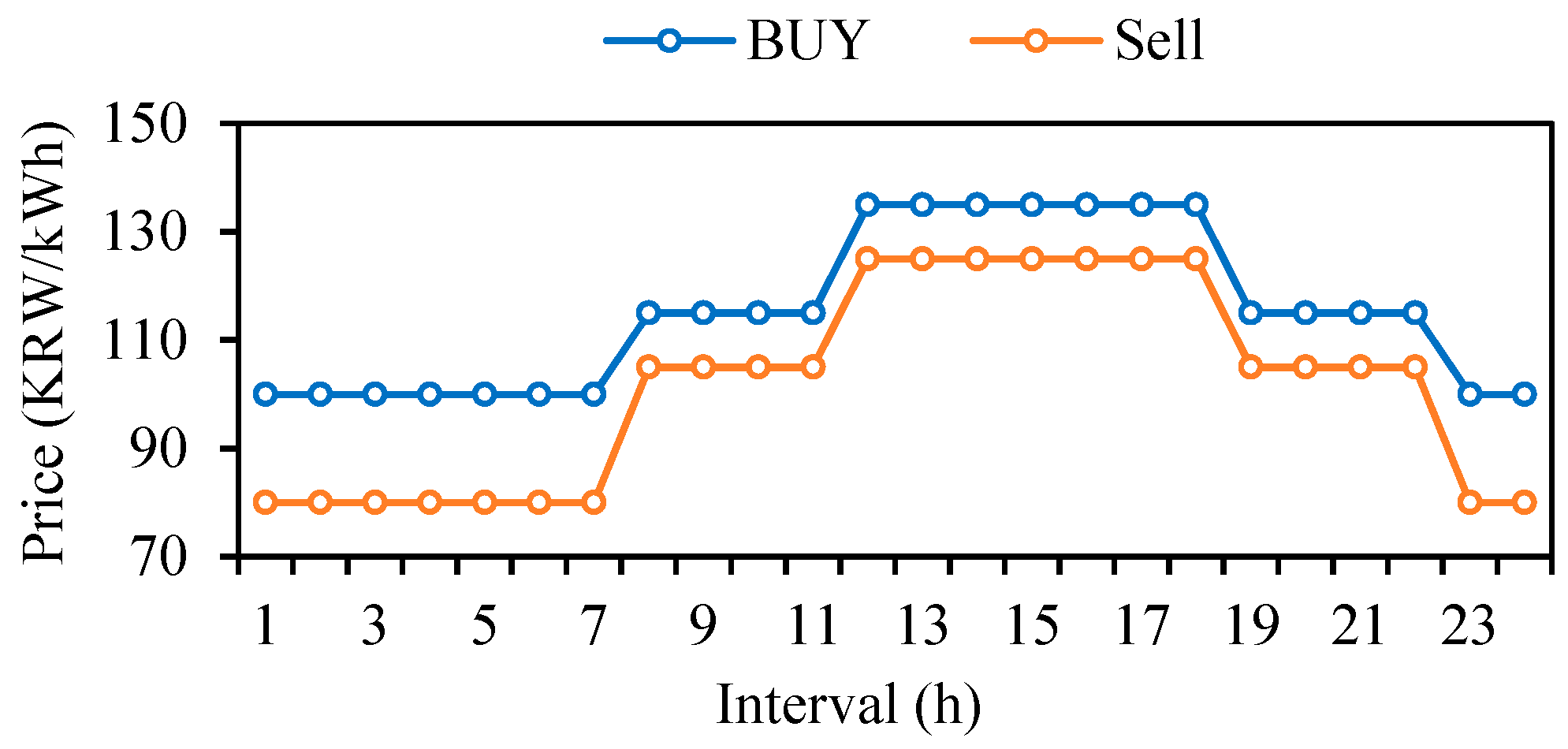
6.1. Input Parameters

The operation cost, capacity, and COP of each energy generation equipment used in this study are shown in

Table 1. Input parameters for energy supply facilities.

Parameters	Cost (KRW/kWh)	Capacity (kWh)	COP
CHP	130	150	2
HOB	70	200	1
Chiller	20	500	0.7
Chiller_B	20	50	0.7
EHP_heat	-	500	1.6
EHP_cooling	-	500	2

. The time-of-use (TOU) day-ahead market price signals are taken as inputs and are shown Figure 8. Initial values, loss rates, and capacity of BESS and TESS are shown in

Table 2. Battery energy storage system (BESS) and thermal energy storage system (TESS) parameters.

Parameters	Initial	Capacity	Charging Loss	Discharging Loss	Loss per Hour
	(kWh)	(kW)	(%)	(%)	(%)
BESS	10	50	5	5	-
TESS	1000	100	-	-	4
TESS_B	100	10	-	-	4

.

Table 3. Control parameters in greenhouse.

Parameters	Humidity	Lighting	CO2	Temperature
	(%)	(W/m2)	(ppm)	(°C)
Min.	65	200	700	14
Max.	85	-	1000	30

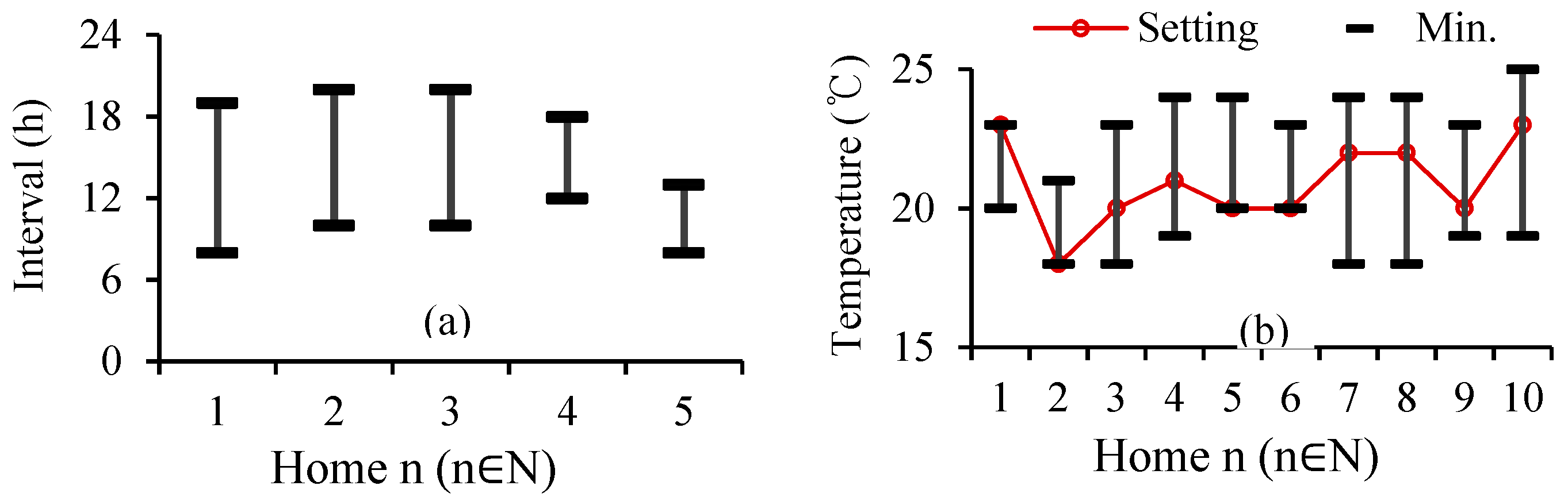
shows the acceptable bounds of the control parameters for the greenhouse. The temperature of each household in the building must be controlled within the setting bounds.

Table 4. Temperature control of each household in building.

Household No.	1	2	3	4	5	6	7	8	9	10
Sleeping time (t)	23	24	24	23	23	22	23	24	23	22
Waking time (t)	6	7	7	8	6	6	8	7	7	6

shows the sleeping and waking up times of the residents in each household. During sleeping time, the temperature should be controlled within 21–22 °C. Figure 9a shows the time when the residents are out of the household and the temperature bound should be controlled within 0–30 °C. When the residents arrive at the household, temperature of each household should be controlled to the preset temperature level by the resident. In all other cases, temperature bounds should be controlled as shown Figure 9b, which is set by the residents of each household.

6.2. Summer Season

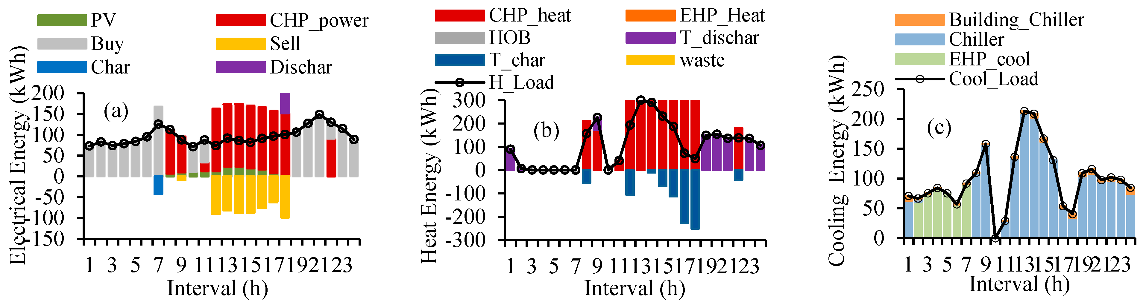
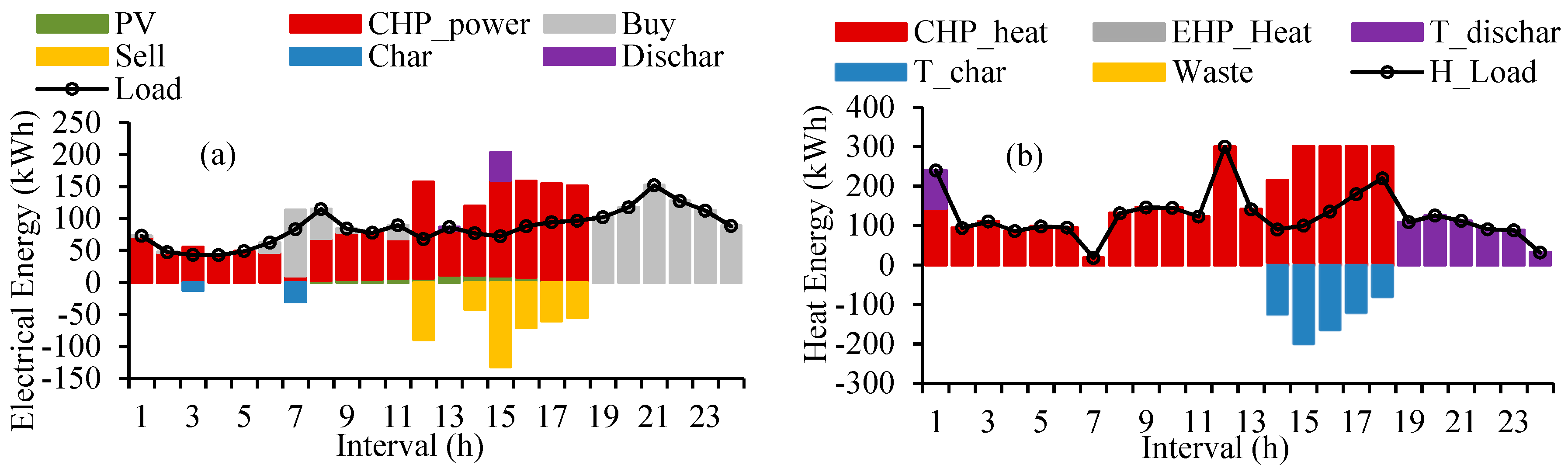
Energy balance of power, heat, and cooling are shown in Figure 10. In the off-peak and mid-peak periods, the price for buying electricity from the utility grid is lower than the generation cost of the CHP. During off-peak period, there is no heat load, except time interval 1, therefore, power is purchased from the utility grid during these intervals. During mid-peak hours, CHP is operated to fulfil the heat load demand. For economical operation, BESS charges power in the off-peak period and discharges the charges power at the peak period. In the peak period, the buying price from the utility grid is higher than the CHP price, therefore, the CHP is operated to its fullest. Excess heat is stored in the TESS and surplus power is sold to the utility grid. PV generates the power during intervals 8–18. In summer, heat energy is used for fulfilling the cooling demand of the greenhouse using chillers. TESS stores and releases heat for optimal heat energy management. The cooling energy is supplied mainly through the chiller, which utilizes the heat generated by the CHP, as shown in Figure 10c.

EHP is only used when there is shortage of heat energy due to higher generation cost. The exhaust heat produced due to the operation of air-conditioner in the building is used by the chillers to produce cooling energy for the greenhouse.

Table 5. Equipment usage for environment control during summer season in greenhouse.

Interval (t)	1	2	3	4	5	6	7	8	9	10	11	12
Cooling pipe valve (%)	79.8	72.1	73.9	73.9	73.8	64.7	89.8	100	100	0	10.1	37.3
Air circulation fan (On/Off)	1	1	0	0	0	1	1	0	1	0	1	1
CO2 injection (kWh)	5	5	0	0	0	5	5	0	5	0	5	5
Dehumidifier (kWh)	1.4	1.3	1.3	1.3	1.2	1.4	1.3	1.3	1.3	0.8	1.2	1.5
Artificial light (kWh)	4	4	4	4	4	4	2.2	0.4	0	0	0	0
Interval (t)	13	14	15	16	17	18	19	20	21	22	23	24
Cooling pipe valve (%)	53.3	50.7	39.8	31.1	11.5	13.3	100	100	100	100	94.3	85.1
Air circulation fan (On/Off)	1	1	1	1	0	0	1	1	0	0	1	0
CO2 injection (kWh)	5	5	5	4.04	0	0	5	3.27	0	0	4.13	0
Dehumidifier (kWh)	1.2	1.2	1.2	1.3	1.3	1.5	1.5	1.4	1.3	1.2	1.4	1.2
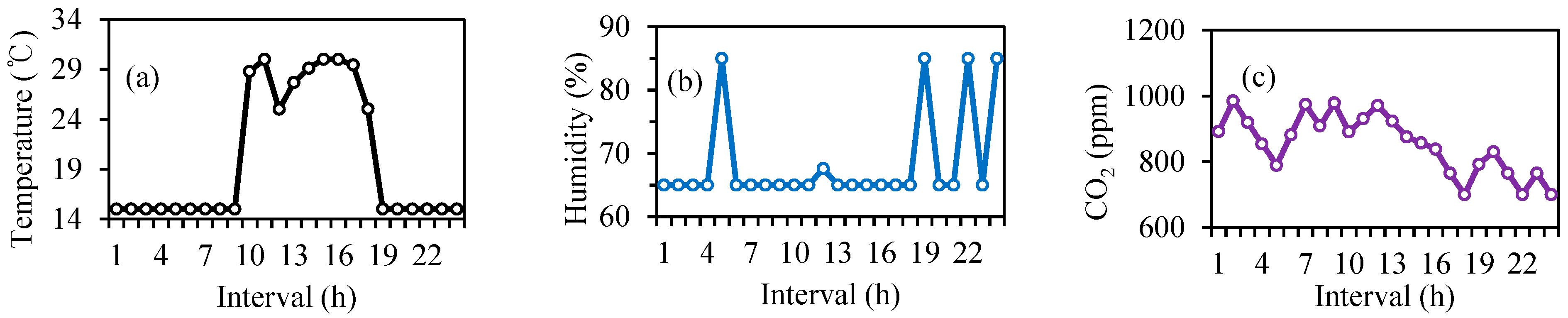
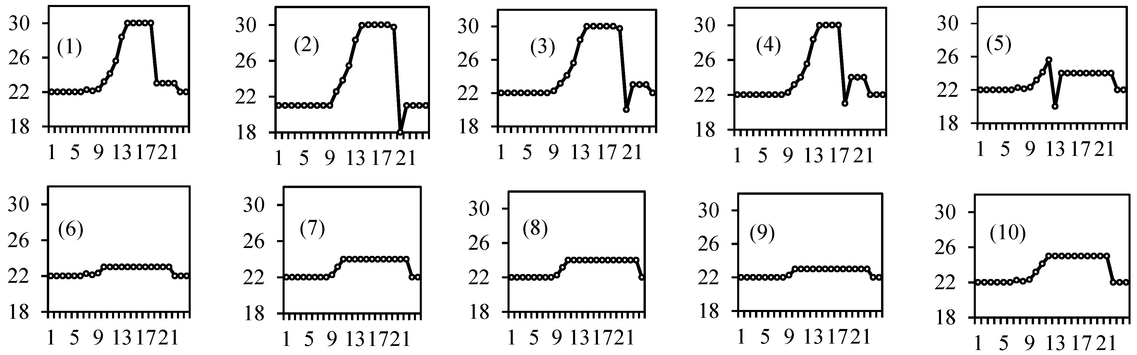
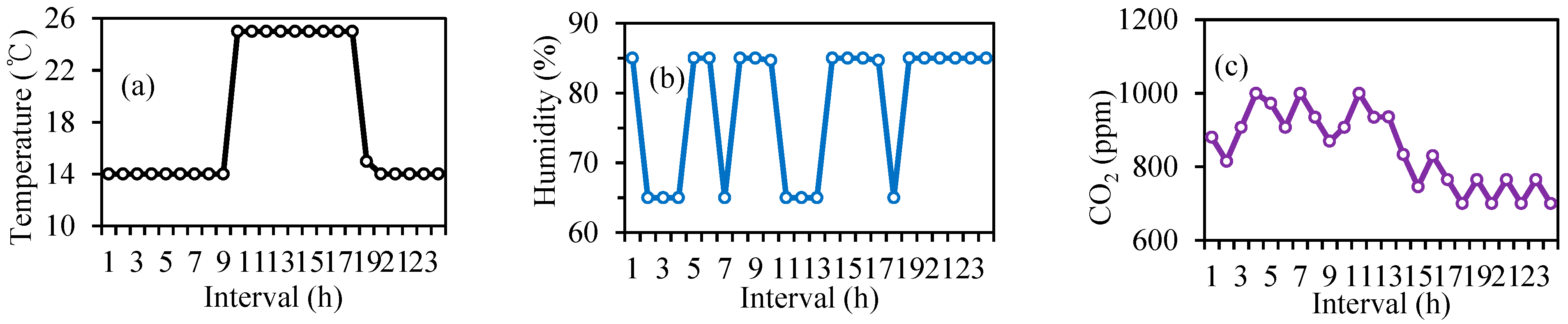
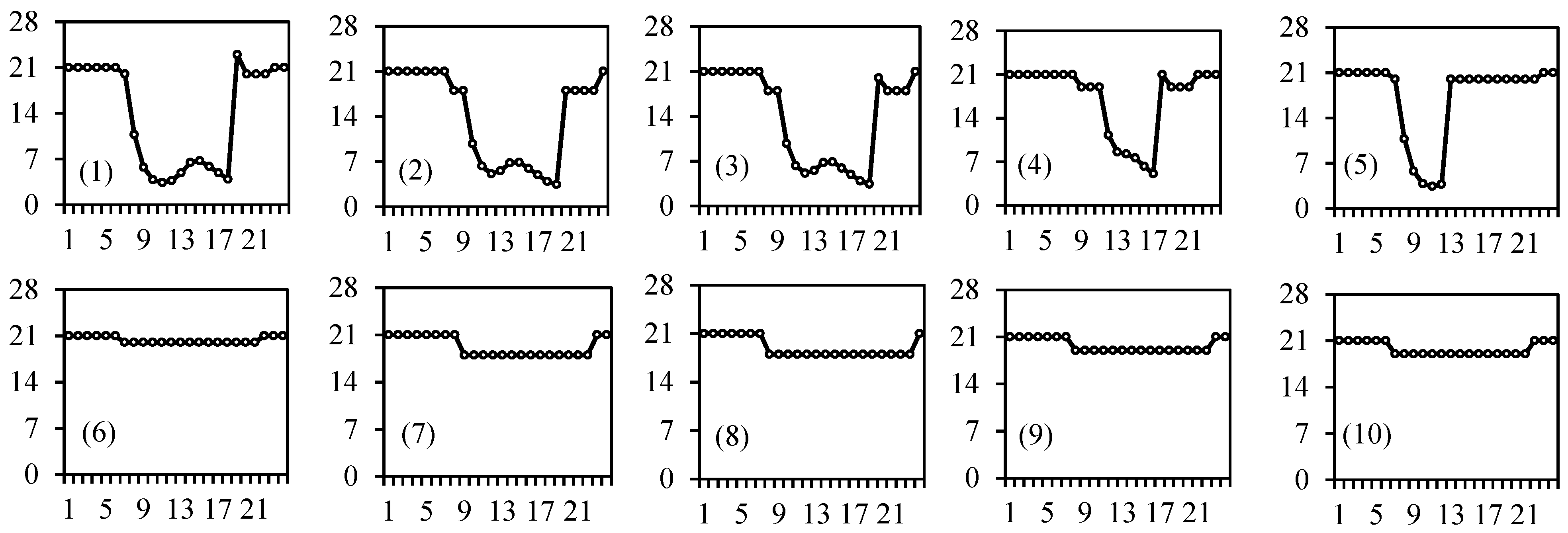
Artificial light (kWh)	0	0	0	0	0	3.1	4	4	4	4	4	4

shows the schedule of equipment operating for maintaining the indoor environment of the greenhouse. Since the outside temperature is higher in the summer, the cooling pipe valve is used frequently for maintaining a proper growth temperature. When carbon dioxide is injected, air circulation fans are used to distribute it evenly inside the greenhouse. In the greenhouse, the internal humidity is increased due to the transpiration of crops, so the dehumidifier is used for controlling the humidity. Artificial lights are mainly used when the solar radiations are not sufficient (early morning and night time). As a result, the temperature, humidity, lighting, and carbon dioxide concentration of the greenhouse can be controlled within the set range as shown in Figure 11. The temperature of each household in the building is also controlled within the defined range, as shown in Figure 12. The residents of building 1 to 5 go out and come back as specified in Figure 9a. Therefore, a significant difference in temperature during the presence and absence of residents can be observed from Figure 12. Additionally, when the residents return household, the room temperature is set to the pre-set value (Figure 9b), as shown in Figure 12. However, at least one of the residents stayed in the household all the time for households 6 to 10. Therefore, only the temperature difference between sleeping and awake times can be observed, as specified in Table 4.

6.3. Winter Season

Energy balance of power and heat are shown in Figure 13a,b, respectively. During the winter season, cooling is not required and more heating is required to maintain the indoor climate for crops. Similarly, no cooling is required in the building, therefore, results of the cooling energy are not shown in the simulation results. In the initial intervals of the day, the CHP generation amount is controlled by the heat load due to the lower market selling prices, as shown in Figure 13a. During peak price intervals, CHP is operated fully and an excess of heat is stored in the TESS, which is used at the last intervals of the day. During the last off-peak hours, TESS is discharged to fulfil the heat requirements of the microgrid, as shown in Figure 13b. During the off-peak intervals (last six intervals), electricity is bought from the utility grid due to lower market price and the ability of TESS to feed the heat loads.

Table 6. Equipment usage for environment control during winter season in greenhouse.

Interval (t)	1	2	3	4	5	6	7	8	9	10	11	12
Heating pipe valve (%)	19.1	18.8	16.7	15.1	13.7	15.5	23	12.3	11.6	44.4	58.4	35.7
Air circulation fan (On/Off)	1	0	1	1	1	0	1	0	0	1	1	0
CO2 injection (kWh)	4.62	0	5	5	1.2	0	5	0	0	3.26	5	0
Dehumidifier (kWh)	1.32	1.4	1.3	1.3	1.2	1.3	1.4	1.2	1.3	0.9	1.5	1.3
Artificial light (kWh)	4	4	4	4	4	4	3.1	2.2	1.3	1.3	0.4	0.4
Interval (t)	13	14	15	16	17	18	19	20	21	22	23	24
Heating pipe valve (%)	18	14.4	21	29.2	40	47.8	16	17	16.8	18.9	18.5	27
Air circulation fan (On/Off)	1	0	0	1	0	0	1	0	1	0	1	0
CO2 Injection (kWh)	3.28	0	0	5	0	0	4.14	0	4.14	0	4.14	0
Dehumidifier (kWh)	1.3	1.1	1.3	1.3	1.3	1.5	1.5	1.32	1.3	1.3	1.3	1.3
Artificial light (kWh)	0	0	0	0	1.75	3.55	4	4	4	4	4	4

shows the schedules of equipment operating for maintaining the indoor environment of the greenhouse. Since the outside temperature is lower in winter, the heating pipe valve is operated frequently to maintain a proper growth temperature. Similarly, in the winter season, the use of artificial light is also more frequent due to shorter day time.

It can be observed from Figure 14 that the indoor control parameters of the greenhouse are within the specified ranges throughout the day. Similarly, the indoor temperature of all the ten households is also within the specified range by the residents (Figure 9 and Table 4), as shown in Figure 15. Similar to the summer season, residents of households 1 to 5 are not at home throughout the day, while at least one resident of households 6 to 10 is at home throughout the day.

7. Conclusions

In order to minimize the operation cost, this paper has proposed an optimal operation method for building a microgrid with rooftop greenhouses. The proposed operation scheme has been realized by using a MAS in a single PC. Simulation results have proved the economic feasibility of integrating the greenhouse in building microgrid. The waste heat generated by the air conditioners of the building is used for fulfilling the cooling demand of the greenhouse via a chiller, which is otherwise wasted. The operation cost has reduced due to better utilization of the CHP and EHP units while reducing waste heat. The coupling effect of the energy demand in the building and the greenhouse is analyzed for two seasons of a year, i.e., summer and winter. The operation cost of the summer season is 27% higher than that of the winter season due to the higher magnitude of the cooling load. The amount of power usage in the summer season is 13% higher than that of the winter season due to utilization of air conditioners and EHP units. The operating rate of the cooling pipe in summer was three times higher than that of the heating pipe in winter.

In this study, forecasted values of wind speed, solar irradiations, and loads are utilized. However, these parameters are subjected to uncertainties. Therefore, the consideration of uncertainties in the proposed model could be a valuable extension of this article. Similarly, the islanded operation of the microgrid along with the failure of local equipment also need to be considered in future studies.

References

- Organization for Economic Cooperation and Development. Agence Internationale de L’énergie. Energy Technology Perspectives 2012: Pathways to a Clean Energy System; OECD/IEA: Paris, France, 2012. [Google Scholar]
- Galvin, R.; Kurt, Y. Perfect Power: How the MicroGrid Revolution Will Unleash Cleaner, Greener, More Abundant Energy; McGraw Hill Professional: New York, NY, USA, 2008. [Google Scholar]
- Lasseter, R.H. Smart distribution: Coupled microgrids. Proc. IEEE 2011, 99, 1074–1082. [Google Scholar] [CrossRef]
- Clastres, C. Smart grids: Another step towards competition, energy security and climate change objectives. Energy Policy 2011, 39, 5399–5408. [Google Scholar] [CrossRef] [Green Version]
- Lasseter, R.H.; Paigi, P. Microgrid: A conceptual solution. In Proceedings of the 2004 IEEE 35th Annual Power Electronics Specialists Conference, Aachen, Germany, 20–25 June 2004; pp. 4285–4290. [Google Scholar]
- Katiraei, F.; Iravani, R.; Hatziargyriou, N.; Dimeas, A. Microgrids management. IEEE Power Energy Mag. 2008, 6, 54–65. [Google Scholar] [CrossRef]
- Bui, V.H.; Hussain, A.; Kim, H.M. A multiagent-based hierarchical energy management strategy for multi-microgrids considering adjustable power and demand response. IEEE Trans. Smart Grid 2018, 9, 1323–1333. [Google Scholar] [CrossRef]
- Bui, V.H.; Hussain, A.; Kim, H.M. Optimal Operation of Microgrids Considering Auto-Configuration Function Using Multiagent System. Energies 2017, 10, 1484. [Google Scholar] [CrossRef]
- Ou, T.C. A novel unsymmetrical faults analysis for microgrid distribution systems. Int. J. Electr. Power Energy Syst. 2012, 43, 1017–1024. [Google Scholar] [CrossRef]
- Tsui, K.M.; Chan, S.C. Demand response optimization for smart home scheduling under real-time pricing. IEEE Trans. Smart Grid 2012, 3, 1812–1821. [Google Scholar] [CrossRef]
- Ou, T.C.; Hong, C.M. Dynamic operation and control of microgrid hybrid power systems. Energy 2014, 66, 314–323. [Google Scholar] [CrossRef]
- Ou, T.C. Ground fault current analysis with a direct building algorithm for microgrid distribution. Int. J. Electr. Power Energy Syst. 2013, 53, 867–875. [Google Scholar] [CrossRef]
- Zhou, B.; Li, W.; Chan, K.W.; Cao, Y.; Kuang, Y.; Liu, X.; Wang, X. Smart home energy management systems: Concept, configurations, and scheduling strategies. Renew. Sustain. Energy Rev. 2016, 61, 30–40. [Google Scholar] [CrossRef]
- Mohseni, A.; Mortazavi, S.S.; Ghasemi, A.; Nahavandi, A. The application of household appliances’ flexibility by set of sequential uninterruptible energy phases model in the day-ahead planning of a residential microgrid. Energy 2017, 139, 315–328. [Google Scholar] [CrossRef]
- Meegahapola, L.G.; Robinson, D.; Agalgaonkar, A.P.; Perera, S.; Ciufo, P. Microgrids of commercial buildings: Strategies to manage mode transfer from grid connected to islanded mode. IEEE Trans. Sustain. Energy 2014, 5, 1337–1347. [Google Scholar] [CrossRef]
- Ou, T.C. Design of a Novel Voltage Controller for Conversion of Carbon Dioxide into Clean Fuels Using the Integration of a Vanadium Redox Battery with Solar Energy. Energies 2018, 11, 524. [Google Scholar] [CrossRef]
- Ou, T.C.; Lu, K.H.; Huang, C.J. Improvement of transient stability in a hybrid power multi-system using a designed NIDC (Novel Intelligent Damping Controller). Energies 2017, 10, 488. [Google Scholar] [CrossRef]
- Guan, X.; Xu, Z.; Jia, Q.S. Energy-efficient buildings facilitated by microgrid. IEEE Trans. Smart Grid 2010, 1, 243–252. [Google Scholar] [CrossRef]
- Pakr, K.G.; Kim, Y.; Kim, S.; Kim, K.; Lee, W.; Park, H. Building energy management system based on smart grid. In Proceedings of the 2011 IEEE 33rd International Telecommunications Energy Conference (INTELEC), Amsterdam, The Netherlands, 9–13 October 2011; pp. 1–4. [Google Scholar]
- Zhang, D.; Shah, N.; Papageorgiou, L.G. Efficient energy consumption and operation management in a smart building with microgrid. Energy Convers. Manag. 2013, 74, 209–222. [Google Scholar] [CrossRef]
- Tasdighi, M.; Ghasemi, H.; Rahimi-Kian, A. Residential microgrid scheduling based on smart meters data and temperature dependent thermal load modeling. IEEE Trans. Smart Grid 2014, 5, 349–357. [Google Scholar] [CrossRef]
- Nguyen, D.T.; Le, L.B. Optimal bidding strategy for microgrids considering renewable energy and building thermal dynamics. IEEE Trans. Smart Grid 2014, 5, 1608–1620. [Google Scholar] [CrossRef]
- Nikander, J.; Koistinen, M.; Laajalahti, M.; Pesonen, L.; Ronkainen, A.; Suomi, P. Farm information management infrastructures in the future. In Proceedings of the 2015 26th International Workshop on Database and Expert Systems Applications (DEXA), Valencia, Spain, 1–4 September 2015; pp. 104–107. [Google Scholar]
- Kruize, J.W.; Wolfert, S.; Goense, D.; Veenstra, T.; Scholten, H.; Beulens, A. Integrating ICT applications for farm business collaboration processes using FI space. In Proceedings of the 2014 Annual SRII Global Conference (SRII), San Jose, CA, USA, 7–10 June 2014; pp. 232–240. [Google Scholar]
- Khampachua, T.; Wisitpongphan, N. ICT benefit realization for dairy farm management: Challenges and future direction. In Proceedings of the 2014 11th International Joint Conference on Computer Science and Software Engineering (JCSSE), Chonburi, Thailand, 14–16 May 2014; pp. 280–285. [Google Scholar]
- Moon, A.K.; Kim, J.Y.; Zhang, J.; Liu, H.; Son, S.W. Understanding the impact of lossy compressions on IoT smart farm analytics. In Proceedings of the 2017 IEEE International Conference on Big Data (Big Data), Boston, MA, USA, 11–14 December 2017; pp. 4602–4611. [Google Scholar]
- Kolokotsa, D.; Saridakis, G.; Dalamagkidis, K.; Dolianitis, S.; Kaliakatsos, I. Development of an intelligent indoor environment and energy management system for greenhouses. Energy Convers. Manag. 2010, 51, 155–168. [Google Scholar] [CrossRef]
- Luan, X.; Shi, P.; Liu, F. Robust adaptive control for greenhouse climate using neural networks. Int. J. Robust Nonlinear Control 2011, 21, 815–826. [Google Scholar] [CrossRef]
- Vadiee, A.; Martin, V. Energy management strategies for commercial greenhouses. Appl. Energy 2014, 114, 880–888. [Google Scholar] [CrossRef]
- Vadiee, A.; Martin, V. Energy management in horticultural applications through the closed greenhouse concept, state of the art. Renew. Sustain. Energy Rev. 2012, 16, 5087–5100. [Google Scholar] [CrossRef]
- Inayatullah, S. City futures in transformation: Emerging issues and case studies. Futures 2011, 43, 654–661. [Google Scholar] [CrossRef] [Green Version]
- Cohen, N.; Reynolds, K.; Sanghvi, R. Five Borough Farm: Seeding the Future of Urban Agriculture in New York City; Design Trust for Public Space: New York, NY, USA, 2012. [Google Scholar]
- Cerón-Palma, I.; Sanyé-Mengual, E.; Oliver-Solà, J.; Montero, J.I.; Rieradevall, J. Barriers and opportunities regarding the implementation of Rooftop Eco. Greenhouses (RTEG) in Mediterranean cities of Europe. J. Urban Technol. 2012, 19, 87–103. [Google Scholar] [CrossRef]
- Rooftop Greenhouse. Available online: https://myrooff.com/rooftop-greenhouse/ (accessed on 18 July 2018).
- Benis, K.; Gomes, R.; Vicente, R.; Ferrao, P.; Fernandez, J. Rooftop greenhouses: LCA and energy simulation. In Proceedings of the International Conference CISBAT 2015 Future Buildings and Districts Sustainability from Nano to Urban Scale, Lausanne, Switzerland, 9–11 September 2015; pp. 95–100. [Google Scholar]
- Pons Valladares, O.; Nadal, A.; Sanyé-Mengual, E.; Llorach-Massana, P.; Cuerva, E.; Sanjuan-Delmàs, D. Roofs of the future: Rooftop greenhouses to improve buildings metabolism. Procedia Eng. 2015, 123, 441–448. [Google Scholar] [CrossRef] [Green Version]
- Nadal, A.; Llorach-Massana, P.; Cuerva, E.; López-Capel, E.; Montero, J.I.; Josa, A.; Royapoor, M. Building-integrated rooftop greenhouses: An energy and environmental assessment in the mediterranean context. Appl. Energy 2017, 187, 338–351. [Google Scholar] [CrossRef]
- Ercilla-Montserrat, M.; Izquierdo, R.; Belmonte, J.; Montero, J.I.; Muñoz, P.; De Linares, C.; Rieradevall, J. Building-integrated agriculture: A first assessment of aerobiological air quality in rooftop greenhouses (i-RTGs). Sci. Total Environ. 2017, 598, 109–120. [Google Scholar] [CrossRef] [PubMed]
- Nadal, A.; Alamús, R.; Pipia, L.; Ruiz, A.; Corbera, J.; Cuerva, E.; Josa, A. Urban planning and agriculture. Methodology for assessing rooftop greenhouse potential of non-residential areas using airborne sensors. Sci. Total Environ. 2017, 601, 493–507. [Google Scholar] [CrossRef] [PubMed]
- Resinger, M.; Sauer, A. Urban production: Smart rooftop greenhouses as a technology for industrial energy symbiosis. In Proceedings of the 2017 ACEEE Summer Study on Energy Efficiency in Industry, Denver, CO, USA, 15–18 August 2017. [Google Scholar]
- Kim, H.M.; Lim, Y.J.; Kinoshita, T. An intelligent multiagent system for autonomous microgrid operation. Energies 2012, 5, 3347–3362. [Google Scholar] [CrossRef]
- Zhao, P.; Suryanarayanan, S.; Simões, M.G. An energy management system for building structures using a multi-agent decision-making control methodology. IEEE Trans. Ind. Appl. 2013, 49, 322–330. [Google Scholar] [CrossRef]
- Klein, L.; Kwak, J.Y.; Kavulya, G.; Jazizadeh, F.; Becerik-Gerber, B.; Varakantham, P.; Tambe, M. Coordinating occupant behavior for building energy and comfort management using multi-agent systems. Autom. Constr. 2012, 22, 525–536. [Google Scholar] [CrossRef]
- Yang, R.; Wang, L. Development of multi-agent system for building energy and comfort management based on occupant behaviors. Energy Build. 2013, 56, 1–7. [Google Scholar] [CrossRef]
- Chehreghani Bozchalui, M. Optimal operation of energy hubs in the context of smart grids. Ph.D. Thesis, University of Waterloo, Waterloo, ON, Canada, 2011. [Google Scholar]
- Pahuja, R.; Verma, H.K.; Uddin, M. A wireless sensor network for greenhouse climate control. IEEE Pervasive Comput. 2013, 12, 49–58. [Google Scholar] [CrossRef]
- Both, A.J.; Benjamin, L.; Franklin, J.; Holroyd, G.; Incoll, L.D.; Lefsrud, M.G.; Pitkin, G. Guidelines for measuring and reporting environmental parameters for experiments in greenhouses. Plant Methods 2015, 11, 43. [Google Scholar] [CrossRef] [PubMed]
- Spilling, K.; Ylöstalo, P.; Simis, S.; Seppälä, J. Interaction effects of light, temperature and nutrient limitations (N, P and Si) on growth, stoichiometry and photosynthetic parameters of the cold-water diatom Chaetoceros wighamii. PLoS ONE 2015, 10, e0126308. [Google Scholar] [CrossRef] [PubMed]
- Amthor, J.S. Respiration and Crop Productivity; Springer Science & Business Media: Berlin/Heidelberg, Germany, 2012. [Google Scholar]
- Peery, J.A. How Does Humidifity Influence Crop Quality? Available online: https://www.pthorticulture.com/en/training-center/how-does-humidity-influence-crop-quality (accessed on 18 July 2018).
- Hussain, A.; Choi, I.S.; Im, Y.H.; Kim, H.M. Optimal Operation of Greenhouses in Microgrids Perspective. IEEE Trans. Smart Grid 2018. [Google Scholar] [CrossRef]
- Kim, H.M.; Wei, W.; Kinoshita, T. A new modified CNP for autonomous microgrid operation based on multiagent system. J. Electr. Eng. Technol. 2011, 6, 139–146. [Google Scholar] [CrossRef]
- Puga, D. From sectoral to functional urban specialisation. J. Urban Econ. 2005, 57, 343–370. [Google Scholar] [Green Version]
- Sherali, H.D.; Tuncbilek, C.H. A global optimization algorithm for polynomial programming problems using a reformulation-linearization technique. J. Glob. Optim. 1992, 2, 101–112. [Google Scholar] [CrossRef]
- Sherali, H.D.; Adams, W.P. A Reformulation-Linearization Technique for Solving Discrete and Continuous Nonconvex Problems; Springer Science & Business Media: Berlin/Heidelberg, Germany, 2013. [Google Scholar]
- Bozchalui, M.C.; Cañizares, C.A.; Bhattacharya, K. Optimal energy management of greenhouses in smart grids. IEEE Trans. Smart Grid 2015, 6, 827–835. [Google Scholar] [CrossRef]
Figure 1.
Building microgrid configuration.
Figure 2.
Greenhouse configuration.
Figure 3.
Multi-agent configuration of building energy management system (BEMS).
Figure 4.
Multi-agent configuration of greenhouse.
Figure 5.
Multi-agent configuration of building.
Figure 6.
Interaction among different agents.
Figure 7.
Flowchart for operation of the proposed building microgrid with rooftop greenhouse.
Figure 8.
Figure 9.
(a) Residents out stay time; and (b) temperature bounds.
Figure 10.
Energy balance in summer season: (a) power; (b) heat energy; and (c) cooling energy.
Figure 11.
Environmental control of greenhouse in summer season: (a) temperature; (b) humidity; and (c) CO2 concentration.
Figure 12.
Temperature control of each household during summer season in building (X-axis: interval (h), Y-axis: temperature (°C)).
Figure 13.
Energy balance in winter: (a) power; and (b) heat energy.
Figure 14.
Environmental control of greenhouse in winter season: (a) temperature; (b) humidity; and (c) CO2 concentration.
Figure 15.
Temperature control of each household during winter season in building (X-axis: interval (h), Y-axis: temperature (°C)).