Adaptive Higher-Order Sliding Mode Control for Islanding and Grid-Connected Operation of a Microgrid

Abstract

Grid-connected and islanding operations of a microgrid are often influenced by system uncertainties, such as load parameter variations and unmodeled dynamics. This paper proposes a novel adaptive higher-order sliding mode (AHOSM) control strategy to enhance system robustness and handle an unknown uncertainty upper bounds problem. Firstly, microgrid models with uncertainties are established under islanding and grid-connected modes. Then, adaptive third-order sliding mode and adaptive second-order sliding mode control schemes are respectively designed for the two modes. Microgrid models’ descriptions are divided into nominal part and uncertain part, and higher-order sliding mode (HOSM) control problems are transformed into finite time stability problems. Again, a scheduled law is proposed to increase or decrease sliding mode control gain adaptively. Real higher-order sliding modes are established, and finite time stability is proven based on the Lyapunov method. In order to achieve smooth mode transformation, an islanding mode detection algorithm is also adopted. The proposed control strategy accomplishes voltage control and current control of islanding mode and grid-connected mode. Control voltages are continuous, and uncertainty upper bounds are not required. Furthermore, adjustable control gain can further whittle control chattering. Simulation experiments verify the validity and robustness of the proposed control scheme.

1. Introduction

A microgrid, which mainly includes a direct current (DC) form, an alternate current (AC) form, and an AC-DC form, is a small power system consisting of a distributed microsource, energy storing device, energy conversion device, and a load and control protection device [1]. It can provide clean energy for a remote area, island or city community and achieve combined cooling, heating, and power [2,3]. Microgrids have become a new driving force for the development of distributed renewable energy sources [4]. Microgrid operations consist of a grid-connected mode and an islanding mode. In grid-connected mode, voltage and frequency references are provided by the main grid and each distributed generation unit (DGu) achieves active power and reactive power regulation via current control. In islanding mode, voltage and frequency reference are maintained by the main DGu of a microgrid [5].

In the form of DC distribution, distributed microsources of a DC microgrid are merged together and coordinately controlled. Study on DC microgrid control has procured plentiful and substantial progeny [6,7]. However, for the AC microgrid, microgrid voltage control under the two modes is one of the key technologies for achieving safe and stable operation [8,9]. Many control methods are applied in the microgrid operation [10]. Droop control is a common voltage control method under islanding mode [11,12]. However, conventional droop control has some drawbacks, such as slow transient response and high dependence of filter impedance [13]. Dynamic load is also not included in the control loop, of which rapid or large variation may result in instability of voltage or frequency. Moreover, this method is not robust for microgrid parameters perturbation and external disturbance and can only make the microgrid steadily operate around a small operating region, which severely restricts the popularization and application of microgrid technology [14].

Sliding mode control, viewed as a variable structure nonlinear control method, has many advantages, such as rapid response and insensitivity to parametric variation and disturbance. It is suitable for power system robust control. Recently, some attempts have been made to study microgrid sliding mode control under grid-connected mode or islanding mode and have achieved corresponding robustness with parametric variation and external disturbance [15,16,17,18,19]. However, this literature does not only have its own drawbacks, such as single mode operation and lack of mode transformation strategy but also has the common problem of first-order sliding mode, which is a notorious control chattering phenomenon. Chattering can severely shorten the service life of power electronic devices in a microgrid system.

Higher-order sliding mode (HOSM), with higher sliding accuracy, is suitable for high relative degree systems and can further restrain chattering by means of increasing system relative degree and hiding discontinuous term under time derivative of control term [20,21]. HOSM control has been a hot topic and widely applied in power system control [22,23]. Some scholars have attempted to study HOSM control for microgrid operation. Cucuzzella et al. [24] designed a suboptimal second-order sliding mode control scheme for islanding operation of a master-slave microgrid. Yet, the system relative degree was also two, which signified that the output control voltage of the voltage source inverter (VSI) was discontinuous and that the inhibitory effect of chattering is poor. In [25], third-order sliding mode control for the microgrid inverter was accomplished based on a combined linear sliding surface. However, the system only had asymptotic stability. Finite time stability for islanding operation was achieved based a third-order sliding mode control scheme in [26]. However, the microgrid model (controlled object) was treated as a black box in this method, which led to conservative parameter choice. Though control action can be continuous by artificially increasing relative degree, conservative control parameters will undoubtedly aggravate chattering. Meanwhile, an islanding mode detection algorithm is not mentioned which may extend transient response and cannot comply with IEEE Std. 1547-2003 [27].

Additionally, uncertainty upper bounds of the microgrid are supposed to be known in all aforementioned studies. However, no matter what, it is difficult to factually estimate the modeling error of VSI or system parameters. Conservative parameter choice may increase control action and intensify chattering phenomenon. Thus, HOSM control combining with an adaptive control gain method can fit well with this situation. Control gain can be adaptively regulated according to the amplitude of uncertainty upper bounds; meanwhile real HOSM is established. Paper [28] proposes an adaptive suboptimal second-order sliding mode control method for grid-connected operation. The control gain can be regulated according to uncertainty variation and control chattering is greatly whittled. However, the known part of the system model is viewed as uncertainty which increasing the controller burden.

In this paper, a novel AHOSM control strategy is proposed for islanding and grid-connected operations of a microgrid. Mathematic models of microgrids under islanding mode and grid-connected mode are established first. The HOSM control problem is then converted to a finite time stability problem under islanding mode and adaptive third-order sliding mode voltage controller is designed combining homogeneous control law with adaptive sliding mode control law. In grid-connected mode, an adaptive second-order sliding mode control scheme is proposed to track current demand. Microgrid control under islanding and grid-connected modes are both based on adaptive higher-order sliding mode (AHOSM), which can conquer unknown uncertainty upper bounds, whittle control chattering, and achieve voltage or current regulation. Islanding event detection and reconnection algorithm is also adopted to achieve smooth mode transformation.

The paper is organized as follows: Section 2 is microgrid modeling. The control strategy including adaptive third-order sliding mode control for islanding mode, adaptive second-order sliding mode control for grid-connected mode, and an islanding event detection and reconnection algorithm is proposed in Section 3. Section 4 presents some simulation results. Finally some, concluding remarks are given in Section 5.

2. Microgrid Modeling

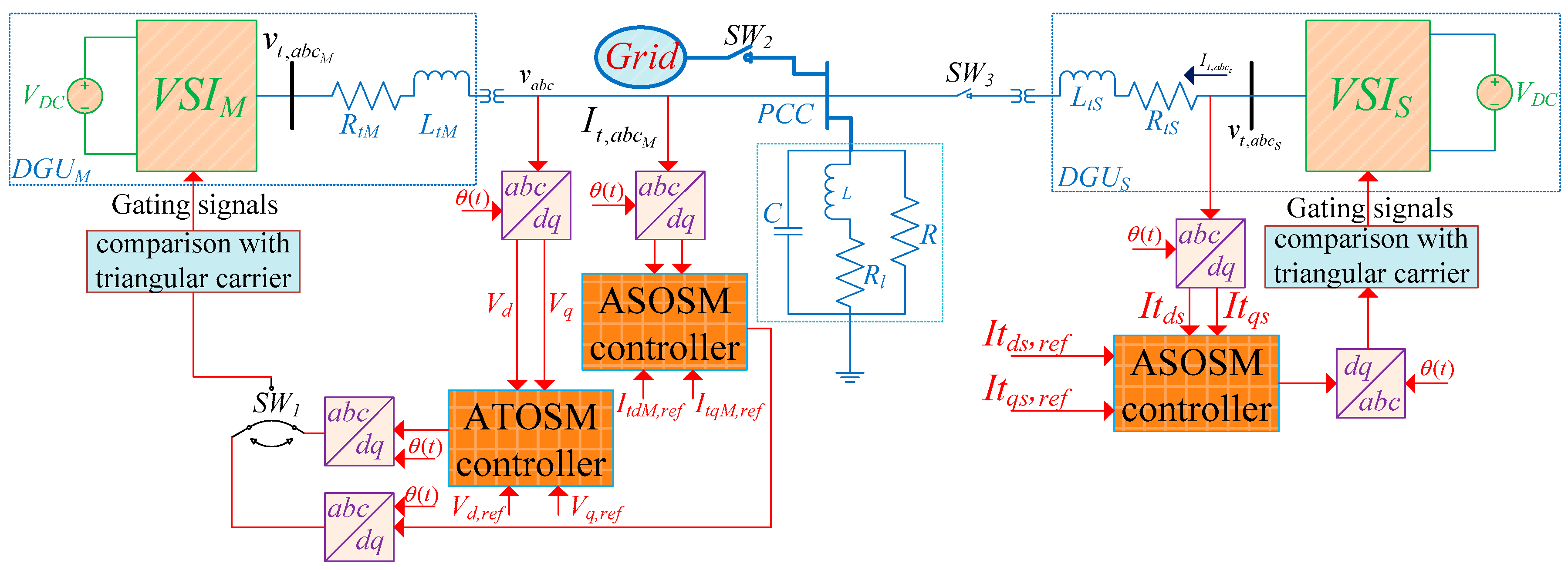
A single-line diagram of a master-slave microgrid with nDGus [26,29] is shortly shown in Figure 1. Each microsource is a generally renewable energy type and is represented by a DC voltage source, which is connected with the main grid via VSI, RL filter, and PCC. Three-phase balanced RCL load is connected with the microgrid.

Voltage magnitude and frequency of PCC are determined by the main grid under grid-connected mode. Thus, the microgrid is stiff synchronous with the main grid, and the reference angle of Park transformation is provided by PLL. d-q component of load voltage $v_{abc}$ and VSI output current $i_{t,abc}$ are defined as $V_d$, $V_q$, $I_{td}$, $I_{tq}$. PI control is adopted to stabilize $V_q=0$ to lock main grid phase. Then active power and reactive power can be respectively represented as $P=3/2V_d{I}_{td}$, $Q=3/2V_d{I}_{tq}$. Thus, each DGu executes current control to regulate active power and reactive power.

The microgrid turns to islanding mode when breaker SW₂ is open. Due to the power mismatching between the DGu and load, PCC voltage and frequency can acutely deviate from the nominal value at this time. Thus, the DGu should control voltage to track load voltage reference under islanding mode. Park angular transformation is provided by inner oscillator and here it is set as nominal angular frequency ${\omega }_0=2\pi f_0$. The islanding event detection algorithm should be designed to smoothly transfer from grid-connected mode to islanding mode. Hence, the inner oscillator needs PLL to provide phase angle as the initial condition under islanding mode and PCC voltage must be synchronous with the main grid when the microgrid is reconnected.

Figure 1 shows a master-slave microgrid control scheme. All DGus implement current control to achieve active power and reactive power regulation under grid-connected mode. The master DGu switches to voltage control to maintain desired microgrid voltage and frequency, and the slave DGus still regulate power when the islanding event happens.

Considering the symmetrical balanced system shown in Figure 1, according to the Kirchhoff voltage and current law, the DGu governing equations under islanding mode is:

$$\{\begin{array}{l}{i}_{t,abc}=\frac{1}{R}{v}_{abc}+i_{L,abc}+C\frac{d{v}_{abc}}{dt}\\ v_{t,abc}=L_t\frac{d{i}_{t,abc}}{dt}+R_t{i}_{t,abc}+v_{abc}\\ v_{abc}=L\frac{d{i}_{L,abc}}{dt}+R_l{i}_{L,abc}\end{array}$$

(1)

where, $i_{t,abc}$, $v_{abc}$, $i_{L,abc}$, $v_{t,abc}$ are the DGu output current, load current, inductive load L current and VSI output voltage. According to the Clark and Park transformation, every three phase variables in Formula (1) can be represented under a d-q rotating coordinate system:

$$\{\begin{array}{l}{\dot{V}}_d=-\frac{1}{RC}{V}_d+{\omega }_0{V}_q+\frac{1}{C}{I}_{td}-\frac{1}{C}{I}_{Ld}\\ {\dot{V}}_q=-{\omega }_0{V}_d-\frac{1}{RC}{V}_q+\frac{1}{C}{I}_{tq}-\frac{1}{C}{I}_{Lq}\\ {\dot{I}}_{td}=-\frac{1}{L_t}{V}_d-\frac{R_t}{L_t}{I}_{td}+{\omega }_0{I}_{tq}+\frac{1}{L_t}{V}_{td}+\frac{1}{L_t}{u}_{VS{I}_d}\\ {\dot{I}}_{tq}=-\frac{1}{L_t}{V}_q-{\omega }_0{I}_{td}-\frac{R_t}{L_t}{I}_{tq}+\frac{1}{L_t}{V}_{tq}+\frac{1}{L_t}{u}_{VS{I}_q}\\ {\dot{I}}_{Ld}=\frac{1}{L}{V}_d-\frac{R_l}{L}{I}_{Ld}+{\omega }_0{I}_{Lq}\\ {\dot{I}}_{Lq}=\frac{1}{L}{V}_q-{\omega }_0{I}_{Ld}-\frac{R_l}{L}{I}_{Lq}\end{array}$$

(2)

where, $u_{VS{I}_d}$ and $u_{VS{I}_q}$ are matched uncertainties caused by VSI. $x=[V_d,V_q,I_{td},I_{tq},I_{Ld},I_{Lq}]$ is chosen as system state variable, $u=[V_{td},V_{tq}]$ is the control input and $y_I=[V_d,V_q]$ is an output vector. The DGu state space model under islanding mode is:

$$\{\begin{array}{l}{\dot{x}}_1(t)=-\frac{1}{RC}{x}_1(t)+{\omega }_0{x}_2(t)+\frac{1}{C}{x}_3(t)-\frac{1}{C}{x}_5(t)\\ {\dot{x}}_2(t)=-{\omega }_0{x}_1(t)-\frac{1}{RC}{x}_2(t)+\frac{1}{C}{x}_4(t)-\frac{1}{C}{x}_6(t)\\ {\dot{x}}_3(t)=-\frac{1}{L_t}{x}_1(t)-\frac{R_t}{L_t}{x}_3(t)+{\omega }_0{x}_4(t)+\frac{1}{L_t}{u}_1(t)+\frac{1}{L_t}{u}_{VS{I}_d}\\ {\dot{x}}_4(t)=-\frac{1}{L_t}{x}_2(t)-{\omega }_0{x}_3(t)-\frac{R_t}{L_t}{x}_4(t)+\frac{1}{L_t}{u}_2(t)+\frac{1}{L_t}{u}_{VS{I}_q}\\ {\dot{x}}_5(t)=\frac{1}{L}{x}_1(t)-\frac{R_l}{L}{x}_5(t)+{\omega }_0{x}_6(t)\\ {\dot{x}}_6(t)=\frac{1}{L}{x}_2(t)-{\omega }_0{x}_5(t)-\frac{R_l}{L}{x}_6(t)\\ y_{Id}=x_1(t)\\ y_{Iq}=x_2(t)\end{array}$$

(3)

Similarly, the DGu state space model under grid-connected mode is:

$$\{\begin{array}{l}{\dot{x}}_1(t)=-\frac{1}{RC}{x}_1(t)+\omega x_2(t)+\frac{1}{C}{x}_3(t)-\frac{1}{C}{x}_5(t)-\frac{1}{C}{x}_7(t)\\ {\dot{x}}_2(t)=-\omega x_1(t)-\frac{1}{RC}{x}_2(t)+\frac{1}{C}{x}_4(t)-\frac{1}{C}{x}_6(t)-\frac{1}{C}{x}_8(t)\\ {\dot{x}}_3(t)=-\frac{1}{L_t}{x}_1(t)-\frac{R_t}{L_t}{x}_3(t)+\omega x_4(t)+\frac{1}{L_t}{u}_1(t)+\frac{1}{L_t}{u}_{VS{I}_d}\\ {\dot{x}}_4(t)=-\frac{1}{L_t}{x}_2(t)-\omega x_3(t)-\frac{R_t}{L_t}{x}_4(t)+\frac{1}{L_t}{u}_2(t)+\frac{1}{L_t}{u}_{VS{I}_q}\\ {\dot{x}}_5(t)=\frac{1}{L}{x}_1(t)-\frac{R_l}{L}{x}_5(t)+\omega x_6(t)\\ {\dot{x}}_6(t)=\frac{1}{L}{x}_2(t)-\omega x_5(t)-\frac{R_l}{L}{x}_6(t)\\ {\dot{x}}_7(t)=\frac{1}{L_s}{x}_1(t)-\frac{R_s}{L_s}{x}_7(t)+\omega x_8(t)-\frac{1}{L_s}{u}_{gd}(t)\\ {\dot{x}}_8(t)=\frac{1}{L_s}{x}_2(t)-\omega x_7(t)-\frac{R_s}{L_s}{x}_8(t)-\frac{1}{L_s}{u}_{gq}(t)\\ y_{Gd}=x_3(t)\\ y_{Gq}=x_4(t)\end{array}$$

(4)

where $x=[V_d,V_q,I_{td},I_{tq},I_{Ld},I_{Lq},I_{gd},I_{gq}]$ is the state vector, $u=[V_{td},V_{tq}]$ is the control input, $y_G=[I_{td},I_{tq}]$ is the output, $I_{gd}$, $I_{gq}$, $u_{gd}$, $u_{gq}$ are the exchange current and d-q voltages of main grid, $u_{gd}$, $u_{gq}$ are the constant rated nominal values.

3. Control Strategy

The AHOSM control scheme for islanding mode and grid-connected mode operation and the islanding event detection algorithm are presented in this section.

3.1. Adaptive Third-Order Sliding Mode Control for Islanding Operation of the Microgrid

In islanding mode, the master DGu is switched to voltage control manner to maintain voltage stabilization of the microgrid system. Sliding mode variables are chosen as:

$$\{\begin{array}{l}{s}_{Id}=V_{Idref}-V_d\\ s_{Iq}=V_{Iqref}-V_q\end{array}$$

(5)

The system relative degree is easily calculated as two and is artificially increased to three for whittling high frequency oscillation of control variables and alleviating the harmonic influence of the electric signal. Then:

$$\begin{array}{lll}{\stackrel{⃛}{s}}_{Id}& =& -\frac{2{\omega }_0}{RC}{\dot{x}}_2-\left(\frac{1}{R{C}^2}+\frac{R_t}{L_{t}C}\right)\left(-\frac{1}{L_t}{x}_1(t)-\frac{R_t}{L_t}{x}_3(t)+{\omega }_0{x}_4(t)+\frac{1}{L_t}{u}_1(t)\right)\\ & & -\left(-\frac{1}{R^2{C}^2}+{\omega }_0^2+\frac{1}{L_{t}C}+\frac{1}{LC}\right){\dot{x}}_1+\frac{2{\omega }_0}{C}\left(-\frac{1}{L_t}{x}_2(t)-{\omega }_0{x}_3(t)-\frac{R_t}{L_t}{x}_4(t)+\frac{1}{L_t}{u}_2(t)\right)\\ & & +\left(\frac{1}{R{C}^2}+\frac{R_t}{LC}\right){\dot{x}}_5+\frac{2{\omega }_0}{C}{\dot{x}}_6+\frac{1}{L_{t}C}{\dot{u}}_{VSId}-\left(\frac{1}{R{C}^2}+\frac{R_t}{L_{t}C}\right)\frac{1}{L_t}{u}_{VS{I}_d}+\frac{2{\omega }_0}{C}\frac{1}{L_t}{u}_{VS{I}_q}\\ & & +\frac{1}{L_{t}C}{\dot{u}}_d+{\stackrel{⃛}{V}}_{Idref}\\ & =& f_{Id}+\Delta f_{Id}+(g_{Id}+\Delta g_{Id})v_d\end{array}$$

(6)

where $v_d={\dot{u}}_d$, $\Delta f_{Id}=\frac{1}{L_{t}C}{\dot{u}}_{VSId}-\left(\frac{1}{R{C}^2}+\frac{R_t}{L_{t}C}\right)\frac{1}{L_t}{u}_{VS{I}_d}+\frac{2{\omega }_0}{C}\frac{1}{L_t}{u}_{VS{I}_q}+\Delta f_{Idv}$, $\Delta f_{Idv}$ is the uncertainty including model error and parameter deviation of $f_{Id}$, $\Delta g_{Id}$ is the uncertain part of $g_{Id}$.

$$\begin{array}{lll}{\stackrel{⃛}{s}}_{Iq}& =& -\left({\omega }_0^2-\frac{1}{R^2{C}^2}+\frac{1}{L_{t}C}+\frac{1}{LC}\right){\dot{x}}_2-\frac{2{\omega }_0}{C}\left(-\frac{1}{L_t}{x}_1(t)-\frac{R_t}{L_t}{x}_3(t)+{\omega }_0{x}_4(t)+\frac{1}{L_t}{u}_1(t)\right)\\ & & +\frac{2{\omega }_0}{RC}{\dot{x}}_1+\left(\frac{1}{R{C}^2}+\frac{R_t}{L_{t}C}\right)\left(-\frac{1}{L_t}{x}_2(t)-{\omega }_0{x}_3(t)-\frac{R_t}{L_t}{x}_4(t)+\frac{1}{L_t}{u}_2(t)\right)+\frac{2{\omega }_0}{C}{\dot{x}}_5\\ & & -\left(-\frac{1}{R{C}^2}-\frac{R_t}{LC}\right){\dot{x}}_6+\frac{1}{L_{t}C}{\dot{u}}_{VSIq}-\frac{2{\omega }_0}{C}\frac{1}{L_t}{u}_{VS{I}_d}+\left(\frac{1}{R{C}^2}+\frac{R_t}{L_{t}C}\right)\frac{1}{L_t}{u}_{VS{I}_q}\\ & & +{\stackrel{⃛}{V}}_{Iqref}+\frac{1}{L_{t}C}{\dot{u}}_q\\ & =& f_{Iq}+\Delta f_{Iq}+(g_{Iq}+\Delta g_{Iq})v_q\end{array}$$

(7)

where $v_q={\dot{u}}_q$, $\Delta f_{Iq}=\frac{1}{L_{t}C}{\dot{u}}_{VSIq}-\frac{2{\omega }_0}{C}\frac{1}{L_t}{u}_{VS{I}_d}+\left(\frac{1}{R{C}^2}+\frac{R_t}{L_{t}C}\right)\frac{1}{L_t}{u}_{VS{I}_q}+\Delta f_{Iqv}$, $\Delta f_{Iqv}$ is the uncertainty including model error and parameter deviation of $f_{Iq}$, $\Delta g_{Iq}$ is the uncertain part of $g_{Iq}$.

$\Delta f_{Ii}$ and $\Delta g_{Ii}$ (i = d,q) are both bounded and the upper bounds are unknown in the microgrid system and satisfy $|g_{Ii}{}^{-1}\Delta g_{Ii}|\le 1-{\widehat{a}}_{Ii}$, $|\Delta f_{Ii}|\le {\widehat{f}}_{Ii}$, $0<{\widehat{a}}_{Ii}\le 1$. ${\widehat{f}}_{Ii}$ is unknown. Third-order sliding mode control with respect to $s_{Ii}$ is equivalently converted to a finite time stabilization problem:

$$\{\begin{array}{l}{\dot{z}}_{1i}=z_{2i}\\ {\dot{z}}_{2i}=z_{3i}\\ {\dot{z}}_{3i}=f_{Ii}+\Delta f_{Ii}+(g_{Ii}+{\widehat{g}}_{Ii})v_i\end{array}$$

(8)

where $z_{1i}=s_{Ii}$, $z_{2i}={\dot{s}}_{Ii}$ and $z_{3i}={\ddot{s}}_{Ii}$. Considering state feedback control:

$$v_i=g_{Ii}{}^{-1}(-f_{Ii}+{\tau }_i)$$

(9)

Then:

$$\{\begin{array}{l}{\dot{z}}_{1i}=z_{2i}\\ {\dot{z}}_{2i}=z_{3i}\\ {\dot{z}}_{3i}=\Delta g_{Ii}+g_{Ii}{}^{-1}\Delta g_{Ii}{f}_{Ii}+(1+{\overline{g}}_i{}^{-1}\Delta g_{Ii}){\tau }_i\end{array}$$

(10)

To design the auxiliary control law ${\tau }_i$:

$${\tau }_i={\tau }_{Inomi}+{\tau }_{Ismi}$$

(11)

where ${\tau }_{Inomi}$ is adopted to achieve finite time stabilization of the nominal part of Formula (8), ${\tau }_{Inomi}$ is designed as:

$${\tau }_{Inomi}=-c_{I1i}sign(z_{1i})|z_{1i}{|}^{1/7}-c_{I2i}sign(z_{2i})|z_{2i}{|}^{1/5}-c_{I3i}sign(z_{3i})|z_{3i}{|}^{1/3}$$

(12)

As long as the choice of $c_{I1i}$, $c_{I2i}$, $c_{I3i}$ satisfy the Holwitz condition for polynomial $p^3+c_{I3i}{p}^2+c_{I2i}p+c_{I1i}$, the nominal part of Formula (8) can be stabilized in finite time [30].

Sliding mode control item ${\tau }_{Ismi}$ is designed to conquer uncertainty. To define sliding mode function ${\sigma }_{Ii}$:

$$\{\begin{array}{l}{\sigma }_{Ii}=z_{3i}+{\tau }_{auxi}\\ {\dot{\tau }}_{auxi}=-{\tau }_{Inomi}\end{array}$$

(13)

Then:

$${\dot{\sigma }}_{Ii}=(1+g_{Ii}^{-1}\Delta g){\tau }_{Ismi}-g_{Ii}^{-1}\Delta g{f}_{Ii}+\Delta f_{Ii}+g_i^{-1}\Delta g{\tau }_{Inomi}$$

(14)

${\tau }_{Ismi}$ is designed as:

$${\tau }_{Ismi}=-{\beta }_{Ii}sign({\sigma }_{Ii})$$

(15)

Choosing Lyapunov function $V({\sigma }_{Ii})=\frac{1}{2}{\sigma }_{Ii}^2$ to confirm the range of ${\beta }_{Ii}$ so as to stabilize the system.

$$\begin{array}{l}\dot{V}({\sigma }_{Ii})={\sigma }_{Ii}{\dot{\sigma }}_{Ii}={\sigma }_{Ii}\left[(1+g_{Ii}^{-1}\Delta g_{Ii}){\tau }_i-g_{Ii}^{-1}\Delta g_{Ii}{f}_{Ii}+\Delta f_{Ii}-{\tau }_{Inomi}\right]\\ ={\sigma }_{Ii}\left[-(1+g_{Ii}^{-1}\Delta g_{Ii}){\beta }_{Ii}sign({\sigma }_{Ii})-g_{Ii}^{-1}{\widehat{g}}_{Ii}{f}_{Ii}+\Delta f_{Ii}+g_{Ii}^{-1}\Delta g_{Ii}{\tau }_{Inomi}\right]\\ \le {\beta }_{Ii}\left|{\sigma }_{Ii}\right|+(1-{\widehat{a}}_{Ii}){\beta }_{Ii}\left|{\sigma }_{Ii}\right|+(1-{\widehat{a}}_{Ii})\left|f_{Ii}\right|+\Delta f_{Ii}+(1-{\widehat{a}}_{Ii})\left|{\tau }_{Inomi}\right|\end{array}$$

(16)

When ${\beta }_{Ii}>\frac{(1-{\widehat{a}}_{Ii})(|{\tau }_{nomi}|+|f_{Ii}|)+\Delta f_{Ii}+{\eta }_{Ii}}{{\widehat{a}}_{Ii}}$ is satisfied, then:

$$\dot{V}({\sigma }_{Ii})\le {\widehat{a}}_{Ii}{\beta }_{Ii}\left|{\sigma }_{Ii}\right|+\left[(1-{\widehat{a}}_{Ii})(|{\tau }_{nomi}|+|f_{Ii}|)+\Delta f_{Ii}\right]\left|{\sigma }_{Ii}\right|<{\eta }_{Ii}\left|{\sigma }_{Ii}\right|$$

(17)

${\tau }_{Ii}={\tau }_{Inomi}+{\tau }_{Ismi}$ is substituted to Formula (8) and the equivalent closed loop dynamic similar to nominal integral chain is then procured. Finite time stabilization of system (8) is achieved and third-order sliding mode with respect to $s_{Ii}$ is established.

The designed sliding mode control law (14) is based on the assumption that the upper bounds of $\Delta f_{Ii}$ and $\Delta g_{Ii}$ are known. However, unmodeled dynamics and the parameter variation of the factual microgrid system are unknown. Uncertain upper bounds are difficult to determine. Control chattering will be increased and power electronic device may be easily damaged if the upper bounds are conservatively set. Therefore, ${\beta }_{Ii}$ should be constructed to increase or decrease adaptively, according to the uncertainty variation.

The adaptive law of ${\beta }_{Ii}$ is designed as:

$${\dot{\beta }}_{Ii}=\{\begin{array}{ll}{k}_{Ii}|{\mu }_{Ii}{|}^{\frac{1}{4}}{\beta }_{Ii}sign({\mu }_{Ii})& if{\beta }_{Ii}>{\beta }_{Imi}\\ {\rho }_{{\beta }_{Ii}}& if{\beta }_{Ii}\le {\beta }_{Imi}\\ {\mu }_{Ii}=\left|s_{Ii}\right|+{\tau }_t\left|{\dot{s}}_{Ii}\right|+{\tau }_t^2\left|{\ddot{s}}_{Ii}\right|-{\varphi }_i{\tau }_t^3& \end{array}$$

(18)

where ${\varphi }_i>0$, ${\tau }_t$ is the sampling period and ${\rho }_{{\beta }_{Ii}}>0$ can be arbitrarily small to guarantee positive of ${\beta }_{Ii}$.

Theorem 1.

Considering system (3), the control laws are designed as Formulas (9), (11), (12), (15), and adaptive control gain is constructed as (18), then the real third-order sliding mode with respect to$s_{Ii}$will be established in finite time, that is:

$$\left|s_{Ii}\right|\le {\gamma }_{0i}{\tau }_t^3,\left|{\dot{s}}_{Ii}\right|\le {\gamma }_{1i}{\tau }_t^2,\left|{\ddot{s}}_{Ii}\right|\le {\gamma }_{2i}{\tau }_t$$

(19)

where${\gamma }_{0i}\ge 0$,${\gamma }_{1i}\ge 0$,${\gamma }_{2i}\ge 0$. The microgrid system under islanding operation mode achieves finite time stabilization.

Proof. 

to choose the Lyapunov function:

$$V({\sigma }_{Ii})=\frac{1}{2}{\sigma }_{Ii}^2+\frac{1}{2}{({\beta }_{Ii}-{\beta }_{Ii}^{*})}^2$$

(20)

where ${\beta }_{Ii}^{*}$ is upper bounds of ${\beta }_{Ii}$. The uncertainty of the microgrid system is bounded, thus ${\beta }_{Ii}^{*}$ is bounded.

To calculate the first-order time derivative of $V({\sigma }_{Ii})$:

$$\begin{array}{ll}\dot{V}({\sigma }_{Ii})& ={\sigma }_{Ii}{\dot{\sigma }}_{Ii}+{\dot{\beta }}_{Ii}({\beta }_{Ii}-{\beta }_{Ii}^{*})\\ & ={\sigma }_{Ii}{\dot{\sigma }}_{Ii}+k_{Ii}|{\mu }_{Ii}{|}^{\frac{1}{4}}{\beta }_{Ii}sign({\mu }_{Ii})({\beta }_{Ii}-{\beta }_{Ii}^{*})\end{array}$$

(21)

$$\begin{array}{ll}{\sigma }_{Ii}{\dot{\sigma }}_{Ii}& =-{\beta }_{Ii}\left(1+g_{Ii}^{-1}\Delta g_{Ii}\right)\left|{\sigma }_{Ii}\right|+\left[g_{Ii}^{-1}\Delta g_{Ii}\left({\tau }_{nomi}-f_{Ii}\right)+\Delta f_{Ii}\right]{\sigma }_{Ii}\\ & \le -{\widehat{a}}_{Ii}{\beta }_{Ii}\left|{\sigma }_{Ii}\right|+\left[\left(1-{\widehat{a}}_{Ii}\right)\left(\left|{\tau }_{nomi}\right|+\left|f_{Ii}\right|\right)+{\widehat{f}}_{Ii}\right]\left|{\sigma }_{Ii}\right|\end{array}$$

(22)

Consider the following two cases.

Case 1: ${\mu }_{Ii}>0$. This means that third-order sliding mode with respect to $s_{Ii}$ is not established. Control gain ${\beta }_{Ii}$ will increase until ${\beta }_{Ii}>\frac{(1-{\widehat{a}}_{Ii})(|{\tau }_{Inomi}|+|f_{Ii}|)+{\widehat{f}}_{Ii}{}_i+{\eta }_i}{{\widehat{a}}_{Ii}}$ is satisfied, according to adaptive law (18). Then:

$${\sigma }_{Ii}{\dot{\sigma }}_{Ii}\le -{\eta }_{Ii1}\left|{\sigma }_{Ii}\right|$$

(23)

$$\begin{array}{ll}\dot{V}({\sigma }_{Ii})& \le -{\eta }_{Ii1}\left|{\sigma }_{Ii}\right|-k_{Ii}\left|{\mu }_{Ii}{|}^{\frac{1}{4}}{\beta }_{Iim}\right|{\beta }_{Ii}-{\beta }_{Ii}^{*}|\\ & \le -{\eta }_{Ii1}|{\sigma }_{Ii}|-{\eta }_{Ii2}|{\beta }_{Ii}-{\beta }_{Ii}^{*}|\le -{\eta }_{Ii}{\left(\frac{{\sigma }_{Ii}^2}{2}+\frac{|{\beta }_{Ii}-{\beta }_{Ii}^{*}{|}^2}{2}\right)}^{\frac{1}{2}}\\ & \le -{\eta }_{Ii}{V}^{\frac{1}{2}}({\sigma }_{Ii})\end{array}$$

(24)

where ${\eta }_{Ii2}=-k_I{}_i|{\mu }_{Ii}{|}^{\frac{1}{4}}{\beta }_{Iim}$, ${\eta }_{Ii}=\min (\sqrt{2}{\eta }_{Ii1},\sqrt{2}{\eta }_{Ii2})$. Thus, ${\mu }_{Ii}<0$ is satisfied in finite time and real third-order sliding mode with respect to $s_{Ii}$ is established in finite time, satisfying $\left|s_{Ii}\right|\le {\gamma }_{0i}{\tau }_t^3,\left|{\dot{s}}_{Ii}\right|\le {\gamma }_{1i}{\tau }_t^2,\left|{\ddot{s}}_{Ii}\right|\le {\gamma }_{2i}{\tau }_t$.

Case 2 ${\mu }_i<0$. Control gain ${\beta }_{Ii}$ will decrease and satisfy ${\beta }_{Ii}\le \frac{(1-{\widehat{a}}_{Ii})(|{\tau }_{Inomi}|+|f_{Ii}|)+{\widehat{f}}_{Ii}{}_i+{\eta }_i}{{\widehat{a}}_{Ii}}$, according to Formula (18). The signal of $\dot{V}({\sigma }_{Ii})$ is uncertain and closed-loop stability could not reached. Hence, ${\mu }_i$ will exceed zero and ${\beta }_{Ii}>\frac{(1-{\widehat{a}}_{Ii})(|{\tau }_{Inomi}|+|f_{Ii}|)+{\widehat{f}}_{Ii}{}_i+{\eta }_i}{{\widehat{a}}_{Ii}}$ is satisfied. Then $\dot{V}({\sigma }_{Ii})\le -{\eta }_{Ii}{V}^{\frac{1}{2}}({\sigma }_{Ii})$ is achieved.

The establishment of real third-order sliding mode with respect to $s_{Ii}$ means the realization of reference voltage tracking and the tracking error satisfies $\left|s_{Ii}\right|\le {\gamma }_{0i}{\tau }_t^3$. Then the microgrid system under islanding operation mode achieves finite time stabilization. ☐

During the control design process, the involved first-order and second-order time derivative of $s_i$ can be observed via a dynamic gain exact robust differentiator [31].

3.2. Adaptive Second-Order Sliding Mode Control for Grid-connected Operation of the Microgrid

All DGus in the microgrid system work at current control manner under grid-connected operation. The main control objective is to make the VSI output current track the desired value via terminal voltage control and then achieve active and reactive power regulation. Sliding mode variables are chosen as:

$$\{\begin{array}{l}{s}_{Gd}(t)=y_{Gd,ref}-y_{Gd}\\ s_{Gq}(t)=y_{Gd,ref}-y_{Gq}\end{array}$$

(25)

First-order time derivative is deduced as:

$$\begin{array}{ll}{\dot{s}}_{Gd}(t)& =h_d(t,x)+g_d(t,x)u_1(t)\\ & ={\dot{y}}_{Gd,ref}+\frac{1}{L_t}{x}_1(t)+\frac{R_t}{L_t}{x}_3(t)-\omega x_4(t)-\frac{1}{L_t}{u}_1(t)-\frac{1}{L_t}{u}_{VS{I}_d}\end{array}$$

(26)

$$\begin{array}{ll}{\dot{s}}_{Gq}(t)& =h_q(t,x)+g_q(t,x)u_2(t)\\ & ={\dot{y}}_{Gq,ref}+\frac{1}{L_t}{x}_2(t)+\omega x_3(t)+\frac{R_t}{L_t}{x}_4(t)-\frac{1}{L_t}{u}_2(t)-\frac{1}{L_t}{u}_{VS{I}_q}\end{array}$$

(27)

The system relative degrees are one. $I_{Td}$ and $I_{Tq}$ can track the reference values by designing a first-order sliding mode control law for Formulas (26) and (27). However, the control chattering is severe, which is harmful to VSI operation and has a strong impact on the lifetime of a power electronic device. Thus, the system relative degree is enhanced to two, meanwhile, system modeling error and parameter disturbance are considered. Then:

$$\{\begin{array}{l}{\ddot{s}}_{Gi}(t)=f_i(x(t),u(t),d_i(t))+g_i{v}_i(t)\\ {\dot{u}}_i(t)=v_i(t)i=d,q\end{array}$$

(28)

where $v_i(t)$ is the first-order time derivative of actual control variable $u_i(t)$. $f_i$ and $g_i$ are respectively represented as:

$$\begin{array}{l}{f}_d(x(t),u(t),d_d(t))=-\left(\frac{1}{R{L}_{t}C}+\frac{R_t}{L_t^2}\right)x_1(t)+\frac{2\omega }{L_t}{x}_2(t)+\left({\omega }^2+\frac{1}{L_{t}C}-\frac{R_t^2}{L_t^2}\right)x_3(t)\\ +\frac{2\omega R_t}{L_t}{x}_4(t)-\frac{1}{L_{t}C}{x}_5(t)-\frac{1}{L_{t}C}{x}_7(t)+\frac{R_t}{L_t^2}{u}_d(t)-\frac{\omega }{L_t}{u}_q(t)+{\ddot{x}}_{3,ref}(t)+d_d(t)\\ ={\overline{f}}_d+d_d(t)\end{array}$$

(29)

$$\begin{array}{l}{f}_q(x(t),u(t),d_q(t))=-\frac{2\omega }{L_t}{x}_1(t)-\left(\frac{1}{R{L}_{t}C}+\frac{R_t}{L_t^2}\right)x_2(t)-\frac{2\omega R_t}{L_t}{x}_3(t)\\ +\left({\omega }^2+\frac{1}{L_{t}C}-\frac{R_t^2}{L_t^2}\right)x_4(t)-\frac{1}{L_{t}C}{x}_6(t)-\frac{1}{L_{t}C}{x}_8(t)+\frac{\omega }{L_t}{u}_d(t)\\ +\frac{R_t}{L_t^2}{u}_q(t)+{\ddot{x}}_{4,ref}(t)+d_q(t)\\ ={\overline{f}}_q+d_q(t)\end{array}$$

(30)

$$g_d=g_q=-\frac{1}{L_t}$$

(31)

$$d_d(t)=\frac{R_t}{L_t^2}{u}_{SV{I}_d}-\frac{\omega }{L_t}{u}_{SV{I}_q}+\frac{1}{L_t}{\dot{u}}_{SV{I}_d}+{\Delta }_d$$

(32)

$$d_q(t)=\frac{R_t}{L_t^2}{u}_{SV{I}_q}+\frac{\omega }{L_t}{u}_{SV{I}_d}+\frac{1}{L_t}{\dot{u}}_{SV{I}_q}+{\Delta }_q$$

(33)

where ${\Delta }_d$ and ${\Delta }_q$ are the parameter uncertainties. The nominal value and signal of $g_i$ is known in advance. Even so, there is an uncertain part for $L_t$. Thus, Formula (28) can be represented as:

$$\begin{array}{ll}{\ddot{s}}_{Gi}(t)& =f_i(x(t),u(t),d_i(t))+g_i{v}_i(t)\\ & ={\overline{f}}_i(x(t),u(t))+d_i(t)+({\overline{g}}_i+{\widehat{g}}_i)v_i(t)\end{array}$$

(34)

$d_i(t)$ and ${\widehat{g}}_i$ (i = d,q) are both bounded and the upper bounds are unknown in the microgrid system and satisfy $\left|{\overline{g}}_i{}^{-1}{\widehat{g}}_i\right|\le 1-{\overline{a}}_i$, $|d_i(t)|\le {\overline{d}}_i$, $0<{\overline{a}}_i\le 1$. Second-order sliding mode control with respect to $s_{Gi}$ is equivalently viewed as a finite time stabilization problem:

$$\{\begin{array}{l}{\dot{z}}_{1i}=z_{2i}\\ {\dot{z}}_{2i}={\overline{f}}_i(x(t),u(t))+d_i(t)+({\overline{g}}_i+{\widehat{g}}_i)v_i(t)\end{array}$$

(35)

where $z_{1i}=s_{Gi}$ and $z_{2i}={\dot{s}}_{Gi}$. Considering state feedback control:

$$v_i={\overline{g}}_i{}^{-1}(-{\overline{f}}_i(x(t),u(t))+{\tau }_i)$$

(36)

Then:

$$\{\begin{array}{l}{\dot{z}}_{1i}=z_{2i}\\ {\dot{z}}_{2i}=d_i(t)+{\overline{g}}_i{}^{-1}{\widehat{g}}_i{\overline{f}}_i(x(t),u(t))+(1+{\overline{g}}_i{}^{-1}{\widehat{g}}_i){\tau }_i(t)\end{array}$$

(37)

To design:

$${\tau }_{Gi}={\tau }_{Gnomi}+{\tau }_{Gsmi}$$

(38)

where ${\tau }_{Gnomi}$ is adopted to achieve finite time stabilization of the nominal part of Formula (37), ${\tau }_{Gnomi}$ is designed as:

$${\tau }_{Gnomi}=-c_{G1i}sign(z_{1i})|z_{i1}{|}^{1/3}-c_G{}_{2i}sign(z_{2i})|z_{2i}{|}^{1/5}$$

(39)

As long as the choices of $c_{G1i}$, $c_{G2i}$ satisfy the Holwitz condition for polynomial $p^2+c_{G2i}p+c_{G1i}$, the nominal part of Formula (37) can be stabilized in finite time [30].

Sliding mode control item ${\tau }_{Gsmi}$ is designed to conquer uncertainty. To define sliding mode function ${\sigma }_{Gi}$:

$$\{\begin{array}{l}{\sigma }_{Gi}=z_{2i}+{\tau }_{auxi}\\ {\dot{\tau }}_{auxi}=-{\tau }_{Gnomi}\end{array}$$

(40)

$${\dot{\sigma }}_{Gi}=(1+g_i^{-1}\widehat{g}){\tau }_{Gsmi}-g_i^{-1}\widehat{g}{\overline{f}}_i+d_i(t)+g_i^{-1}\widehat{g}{\tau }_{Gnomi}$$

(41)

To design:

$${\tau }_{smi}=-{\beta }_{Gi}sign({\sigma }_{Gi})$$

(42)

Choosing the Lyapunov function $V({\sigma }_{Gi})=\frac{1}{2}{\sigma }_{Gi}^2$ to confirm ${\beta }_G{}_i$ so as to stabilize the system.

$$\begin{array}{l}\dot{V}({\sigma }_{Gi})={\sigma }_{Gi}{\dot{\sigma }}_{Gi}={\sigma }_{Gi}\left[(1+g_i^{-1}{\widehat{g}}_i){\tau }_{Gi}-g_i^{-1}{\widehat{g}}_i\overline{f}+d(t)-{\tau }_{Gnomi}\right]\\ ={\sigma }_{Gi}\left[-(1+g_i^{-1}{\widehat{g}}_i){\beta }_{i}sign({\sigma }_{Gi})-g_i^{-1}{\widehat{g}}_i\overline{f}+d(t)+g_i^{-1}{\widehat{g}}_i{\tau }_{Gnomi}\right]\\ \le {\beta }_i\left|{\sigma }_{Gi}\right|+(1-{\overline{a}}_i){\beta }_i\left|{\sigma }_{Gi}\right|+(1-{\overline{a}}_i)\left|{\overline{f}}_i\right|+{\overline{d}}_i+(1-{\overline{a}}_i)\left|{\tau }_{Gnomi}\right|\end{array}$$

(43)

When ${\beta }_{Gi}>\frac{(1-{\overline{a}}_i)(|{\tau }_{nomi}|+|{\overline{f}}_i|)+{\overline{d}}_i+{\eta }_i}{{\overline{a}}_i}$ is satisfied, then:

$$\dot{V}({\sigma }_{Gi})\le {\overline{a}}_i{\beta }_i\left|{\sigma }_{Gi}\right|+\left[(1-{\overline{a}}_i)(|{\tau }_{Gnomi}|+|{\overline{f}}_i|)+{\overline{d}}_i\right]\left|{\sigma }_{Gi}\right|<{\eta }_i\left|{\sigma }_{Gi}\right|$$

(44)

${\tau }_{Gi}={\tau }_{Gnomi}+{\tau }_{Gsmi}$ is substituted to Formula (37) and an equivalent closed loop dynamic similar to nominal integral chain is then procured. Finite time stabilization of system (37) is achieved and second-order sliding mode with respect to $s_{Gi}$ is established.

The designed sliding mode control law (42) is based on the assumption that the upper bounds of ${\overline{a}}_i$ and ${\overline{d}}_i$ are known. However, unmodeled dynamics and parameter variation of factual the microgrid system are unknown. Uncertain upper bounds are hard to been determined. Control chattering will be increased and the power electronic device may be easily damaged if the upper bounds are conservatively set. Therefore, ${\beta }_{Gi}$ should be constructed to increase or decrease adaptively according to the uncertainty variation.

Adaptive law of ${\beta }_{Gi}$ is designed as:

$${\dot{\beta }}_{Gi}=\{\begin{array}{ll}{k}_{Gi}|{\mu }_{Gi}{|}^{\frac{1}{4}}{\beta }_{i}sign({\mu }_{Gi})& if{\beta }_i>{\beta }_{mi}\\ {\rho }_{{\beta }_i}& if{\beta }_i\le {\beta }_{mi}\\ {\mu }_{Gi}=\left|s_i\right|+{\tau }_t\left|{\dot{s}}_i\right|-{\varphi }_i{\tau }_t^2& \end{array}$$

(45)

Theorem 2.

Considering system (4), the control laws are designed as Formulas (36), (38), (39), (42), and adaptive control gain is constructed as (45), then the real second-order sliding mode with respect to$s_{Gi}$will be established in finite time, that is:

$$\left|s_{Gi}\right|\le {\gamma }_{0Gi}{\tau }_t^2,\left|{\dot{s}}_{Gi}\right|\le {\gamma }_{1Gi}{\tau }_t^{}$$

(46)

where${\gamma }_{0Gi}\ge 0$, ${\gamma }_{1Gi}\ge 0$. The microgrid system under grid-connected operation mode achieves finite time stabilization.

Proof. 

to choose Lyapunov function:

$$V({\sigma }_{Gi})=\frac{1}{2}{\sigma }_{Gi}^2+\frac{1}{2}{({\beta }_{Gi}-{\beta }_{Gi}^{*})}^2$$

(47)

where ${\beta }_{Gi}^{*}$ is upper bounds of ${\beta }_{Gi}$. Microgrid uncertainty under grid-connected mode is bounded, thus ${\beta }_{Gi}^{*}$ is bounded.

To calculate first-order time derivative of $V({\sigma }_{Gi})$:

$$\begin{array}{ll}\dot{V}({\sigma }_{Gi})& ={\sigma }_{Gi}{\dot{\sigma }}_{Gi}+{\dot{\beta }}_{Gi}({\beta }_{Gi}-{\beta }_{Gi}^{*})\\ & ={\sigma }_{Gi}{\dot{\sigma }}_{Gi}+k_{Gi}|{\mu }_{Gi}{|}^{\frac{1}{4}}{\beta }_{Gi}sign({\mu }_{Gi})({\beta }_{Gi}-{\beta }_{Gi}^{*})\end{array}$$

(48)

$$\begin{array}{ll}{\sigma }_{Gi}{\dot{\sigma }}_{Gi}& =-{\beta }_{Gi}\left(1+{\overline{g}}_i^{-1}{\widehat{g}}_i\right)\left|{\sigma }_{Gi}\right|+\left[{\overline{g}}_i^{-1}{\widehat{g}}_i\left({\tau }_{nomi}-{\overline{f}}_i\right)+d_i\right]{\sigma }_{Gi}\\ & \le -{\overline{a}}_i{\beta }_{Gi}\left|{\sigma }_{Gi}\right|+\left[\left(1-{\overline{a}}_i\right)\left(\left|{\tau }_{nomi}\right|+\left|{\overline{f}}_i\right|\right)+{\overline{d}}_i\right]\left|{\sigma }_{Gi}\right|\end{array}$$

(49)

Considering the following two cases.

Case 1: ${\mu }_{Gi}>0$. This means that second-order sliding mode with respect to $s_{Gi}$ is not established. Control gain ${\beta }_{Gi}$ will increase until ${\beta }_{Gi}>\frac{(1-{\overline{a}}_i)(|{\tau }_{nomi}|+|{\overline{f}}_i|)+{\overline{d}}_i+{\eta }_i}{{\overline{a}}_i}$ is satisfied according to adaptive law (45). Then:

$${\sigma }_{Gi}{\dot{\sigma }}_{Gi}\le -{\eta }_{Gi1}\left|{\sigma }_{Gi}\right|$$

(50)

$$\begin{array}{ll}\dot{V}({\sigma }_{Gi})& \le -{\eta }_{Gi1}\left|{\sigma }_{Gi}\right|-k_{Gi}\left|{\mu }_{Gi}{|}^{\frac{1}{4}}{\beta }_{Gim}\right|{\beta }_{Gi}-{\beta }_{Gi}^{*}|\\ & \le -{\eta }_{Gi1}\left|{\sigma }_{Gi}\right|-{\eta }_{Gi2}|{\beta }_{Gi}-{\beta }_{Gi}^{*}|\le -{\eta }_{Gi}{\left(\frac{{\sigma }_{Gi}^2}{2}+\frac{|{\beta }_{Gi}-{\beta }_{Gi}^{*}{|}^2}{2}\right)}^{\frac{1}{2}}\\ & \le -{\eta }_{Gi}{V}^{\frac{1}{2}}({\sigma }_{Gi})\end{array}$$

(51)

where ${\eta }_{Gi2}=-k_G{}_i|{\mu }_{Gi}{|}^{\frac{1}{4}}{\beta }_{Gim}$, ${\eta }_{Gi}=\min (\sqrt{2}{\eta }_{Gi1},\sqrt{2}{\eta }_{Gi2})$. Thus, ${\mu }_{Gi}<0$ is satisfied in finite time and real second-order sliding mode with respect to $s_{Gi}$ is established in finite time satisfying $\left|s_{Gi}\right|\le {\gamma }_{0Gi}{\tau }_t^2,\left|{\dot{s}}_{Gi}\right|\le {\gamma }_{1Gi}{\tau }_t^{}$.

Case 2 ${\mu }_{Gi}<0$. Control gain ${\beta }_{Gi}$ will decrease and satisfy ${\beta }_{Gi}\le \frac{(1-{\overline{a}}_i)(|{\tau }_{nomi}|+|{\overline{f}}_i|)+{\overline{d}}_i+{\eta }_i}{{\overline{a}}_i}$ according to Formula (45). The signal of $\dot{V}({\sigma }_{Gi})$ is uncertain and closed-loop stability could not be reached. Hence, ${\mu }_i$ will exceed zero and ${\beta }_{Gi}\le \frac{(1-{\overline{a}}_i)(|{\tau }_{nomi}|+|{\overline{f}}_i|)+{\overline{d}}_i+{\eta }_i}{{\overline{a}}_i}$ is satisfied. Then $\dot{V}({\sigma }_{Gi})\le -{\eta }_{Gi}{V}^{\frac{1}{2}}({\sigma }_{Gi})$ is achieved.

The involved ${\dot{s}}_{Gi}$ can be observed via a dynamic gain exact robust differentiator [31]. The establishment of real second-order sliding mode with respect to $s_{Gi}$ means the realization of reference voltage tracking and the tracking error satisfies $\left|s_{Gi}\right|\le {\gamma }_{0Gi}{\tau }_t^2$. Then the microgrid system under grid-connected operation mode achieves finite time stabilization. ☐

During the design of HOSM controllers, as soon as the uncertain terms satisfy $|g_{Ii}{}^{-1}\Delta g_{Ii}|\le 1-{\widehat{a}}_{Ii}$, $|\Delta f_{Ii}|\le {\widehat{f}}_{Ii}$, $0<{\widehat{a}}_{Ii}\le 1$, $\left|{\overline{g}}_i{}^{-1}{\widehat{g}}_i\right|\le 1-{\overline{a}}_i$, $|d_i(t)|\le {\overline{d}}_i$, $0<{\overline{a}}_i\le 1$ and the control parameters are chosen according to Formulas (12), (15), (18), (39), (42) and (45), the system robustness can be guaranteed.

3.3. Grid-Connected/Islanding Operations Transformation Strategy

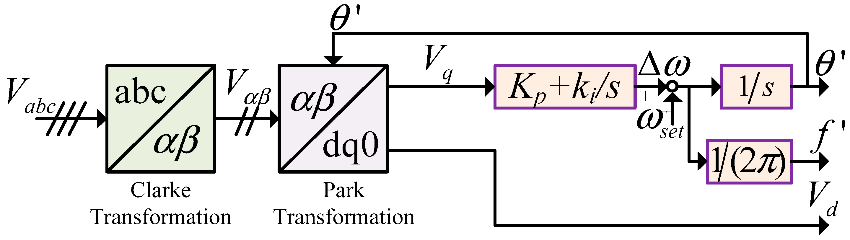
An islanding event must be detected in advance before the microgrid breaks from the main grid. Here, a DQ-PLL method [32] is adopted as shown in Figure 2. DQ-PLL consists of a Clarke transformation, Park transformation, PI regulator and integrator. Vq is propelled to zero via a PI regulator to achieve phase lock. The output of the PI regulator is frequency. DQ-PLL can also track grid frequency. Therefore, voltage and frequency can be used to determine the start of an islanding event. When $0.88<V_{dp.u}<1.1$ and $59.3\mathrm{Hz}<f<60.5\mathrm{Hz}$ cannot both be satisfied, an islanding event is denoted as happening and then VSI is converted to a suitable control mode. Synchronization conditions must firstly also be judged when the DGu is converted to grid-connected mode from islanding mode, which means the amplitude and phase angle of VSI terminal voltage should be coincident with grid voltage. Otherwise, the transient process will be big and the microgrid system may be damaged.

4. Simulation Results

In this section, the proposed control strategy is applied to a master-slave microgrid containing three DGus. System simulation was based on a MATLAB/SimPower Systems tool. Electrical parameters of the microgrid [29] are shown as

Table 1. Electrical parameters of the microgrid.

Quantity	Value	Description
Vdc	1000 V	DC voltage source
fc	10 kHz	PWM carrier frequency
Rt	40 mohm	VSI filter resistance
Lt	10 mH	VSI filter inductance
R	4.33 ohm	Load resistance
L	100 mH	Load inductance
C	1 pF	Load capacity
Rs	0.1 ohm	Grid resistance
f0	60 Hz	Nominal grid frequency
Vn	120 V	Nominal grid phase-voltage
Vd,ref	169.7 V	d-componet of voltage reference
Vq,ref	0 V	q-componet of voltage reference

. Meanwhile, a load which can absorb active power of 25 kW and reactive power of 1.5 kva was added to the system.

After parameter analysis and deliberate simulation, the control parameters are chosen as: $c_{I1d}=3.5\times {10}^3$, $c_{I2d}=4.0\times {10}^3$, $c_{I3d}=6.2\times {10}^3$, $c_{I1q}=2.8\times {10}^3$, $c_{I2q}=4.6\times {10}^3$, $c_{I3q}=5.5\times {10}^3$, $k_{Id}=k_{Id}=0.1$, ${\rho }_{{\beta }_d}=5.2$, ${\rho }_{{\beta }_q}=3.6$, ${\varphi }_d={\varphi }_q=1.0\times {10}^3$ under grid-connected mode, and $c_{G1d}=3.5\times {10}^3$, $c_{G2d}=4.0\times {10}^3$, $c_{G1q}=2.8\times {10}^3$, $c_{G2q}=4.6\times {10}^3$, $k_{Gd}=k_{Gd}=0.1$ under islanding mode. Sampling period for all the simulations is ${\tau }_t=1\times {10}^{-6}s$.

To the authors’ knowledge, other adaptive versions of an HOSM control scheme for microgrid operation for both grid-connected and islanding modes does not currently exist. However, to highlight the superiority of the proposed control scheme, the robust higher-order sliding mode (RHOSM) control method in literature [26] and the PI method were also executed on the microgrid system. The second-order sliding mode control parameters were designed as $U_{i,\max }=4.8\times {10}^7$ and ${\alpha }_i^{\alpha }=0.9$ for the grid-connected mode and the third-order sliding mode control parameters were chosen as ${\alpha }_i=5.2\times {10}^7$, ${\alpha }_{r_d}=1.2\times {10}^{15}$, ${\alpha }_{r_q}=5.0\times {10}^{15}$ for the islanding mode. The control parameters of the PI controllers were turned based on the standard Ziegler-Nichols method. The proportional integral parameters were $K_{pGd}=3.7\times {10}^2$, $K_{pGd}=1.9\times {10}^2$, $K_{IGd}=7.9\times {10}^3$, $K_{IGd}=4.1\times {10}^3$, $K_{pId}=2.9\times {10}^2$, $K_{pId}=2.7\times {10}^2$, $K_{IId}=5.6\times {10}^3$, $K_{IIq}=2.3\times {10}^3$.

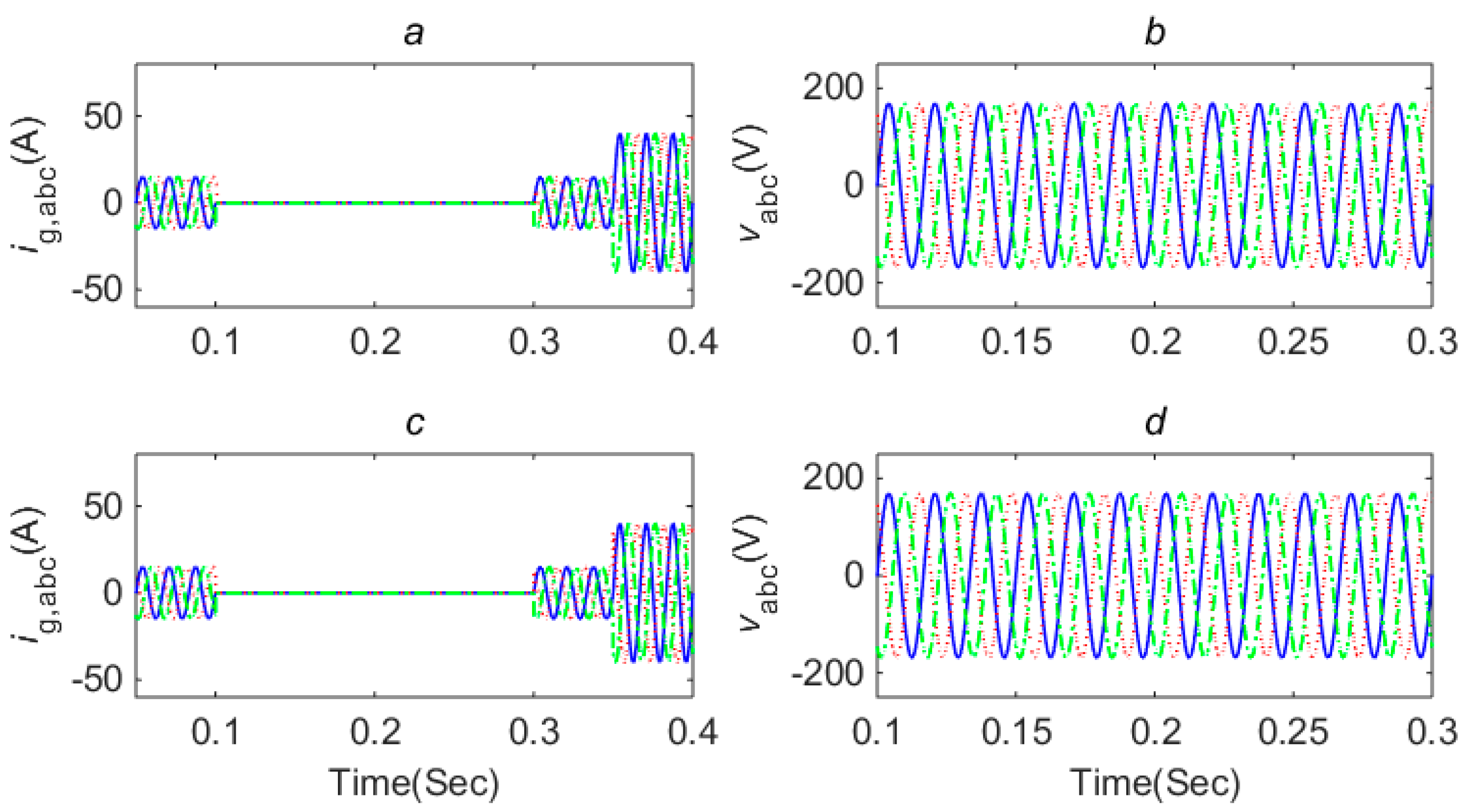
Firstly, the microgrid transforms to islanding mode from grid-connected mode at 0.1 s, and then turns to grid-connected mode at 0.3 s. $I_{Td,ref}$ is set as 90 A from 60 A at 0.35 s. The current exchange between the microgrid and main grid and voltage change of three phase load are shown in Figure 3. As is observed, under both methods, the operation mode transformation was smooth, the response was quick, and the overshoot was small. Mode transformation between voltage control and current control was well done and voltage variation was not influenced by load current variation under grid-connected mode.

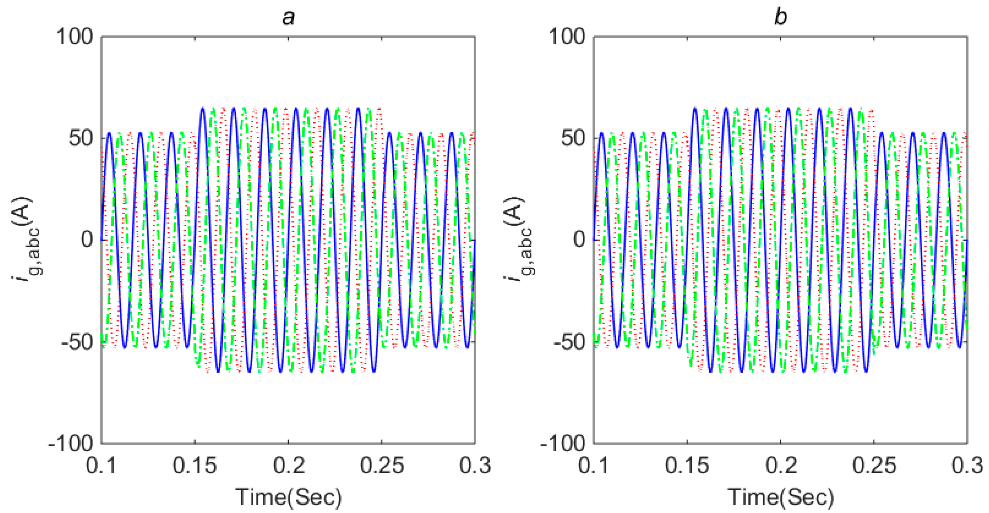
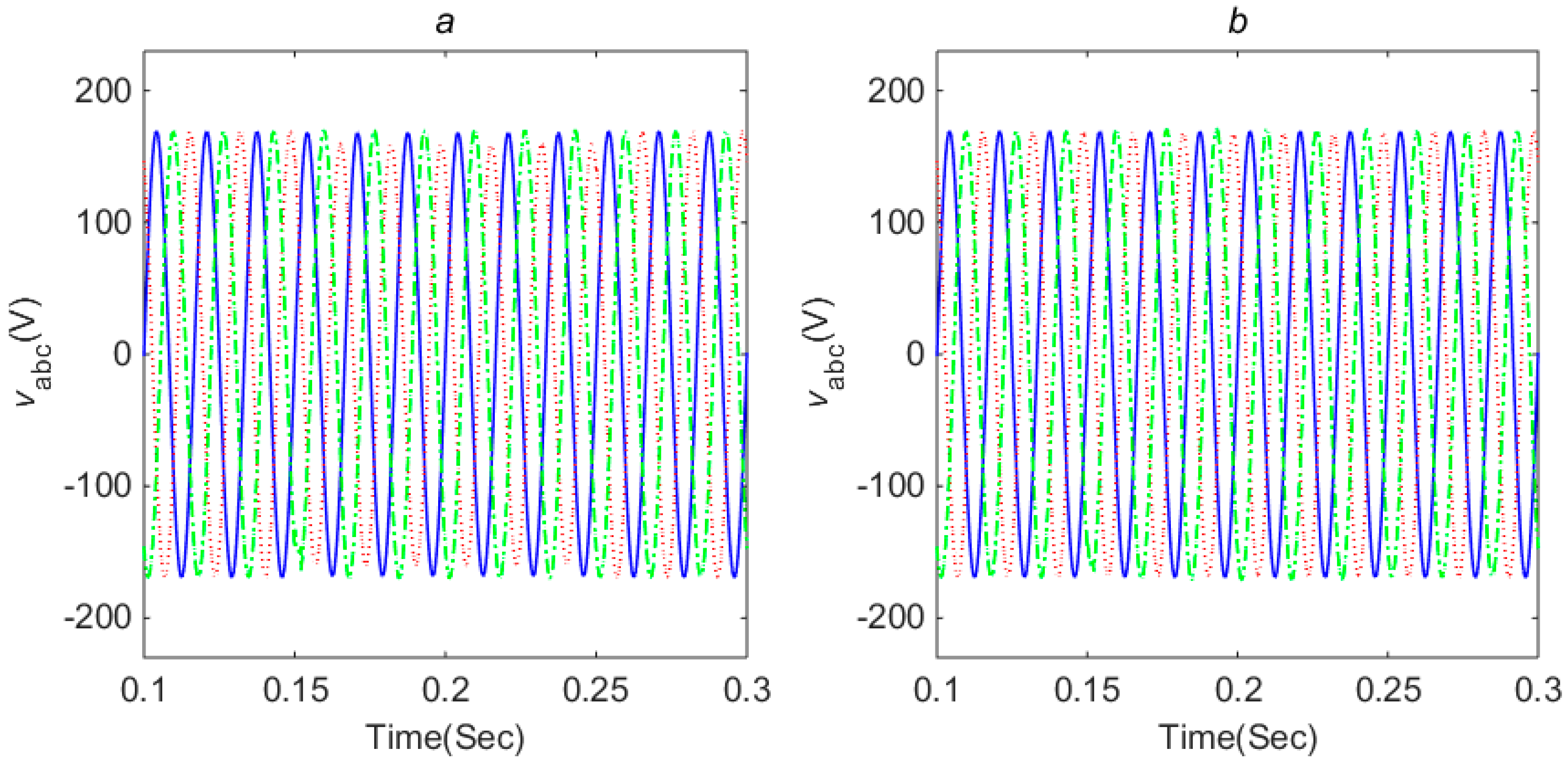
Secondly, the microgrid operated under islanding mode. A three-phase equilibrium load, absorbing 3 kW active power, was added during 0.15–0.25 s. The master DGu output current and load voltage are shown in Figure 4 and Figure 5. Though Figure 4 and Figure 5 indicate the master DGu output current was increased and load voltage was maintained under both the control strategies, the system has better robustness with respect to three-phase equilibrium load under the proposed control strategy when the balanced load is changed.

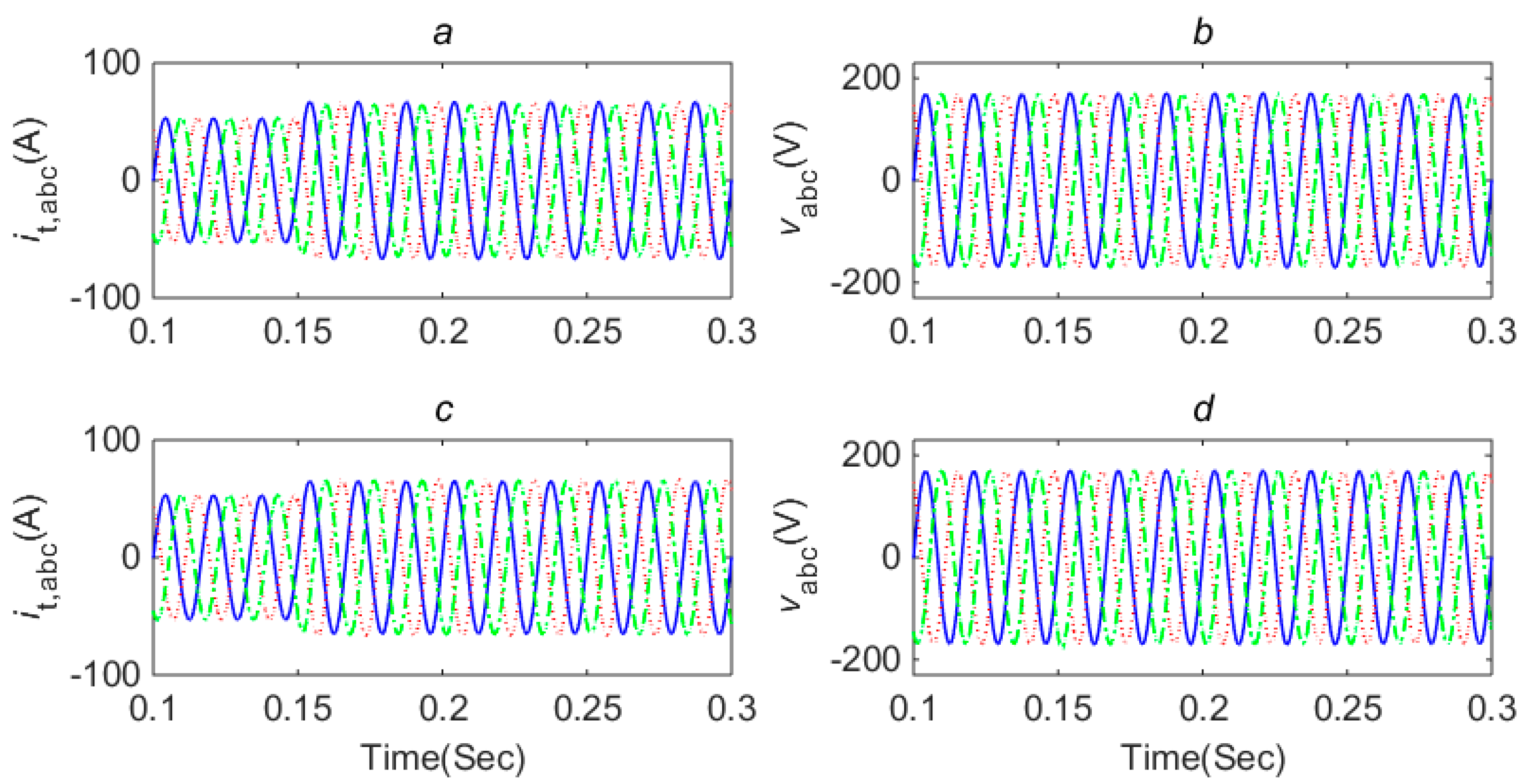
In order to further verify control performances, the balanced load was replaced with an imbalanced load with three phase resistance 5R, 4R, 2R and three phase inductance 0,0,L. Figure 6 shows the output current of the main DGu and load voltage. The approximate calculation formula [33] (46) was adopted to verify conformity of IEEE standard and evaluate the unbalance of PCC voltage.

$$V_{n/p}=\frac{82\sqrt{v_{abe}^2+v_{bce}^2+v_{cae}^2}}{\overline{v}}\times 100\%$$

(52)

where $v_{abe}$, $v_{bce}$, $v_{cae}$ are the line voltage errors and $\overline{v}=(v_a+v_b+v_c)/3$. Then the unbalance ratio $V_{n/p}$ is calculated as 2.3% under the RHOSM method and is 0.02%, which is far lower than the 3% of IEEE standard.

Thirdly, in order to verify robustness for electrical parameters, it was supposed that filter resistance and filter capacitance of the master DGu was changed to 80 mOhm and 20 mH. The simulation is still executed under an unbalance load as shown in Figure 7. It was illustrated that control effect was hardly influenced by filtering the parameter variation within tolerance range, which verifid the good robustness of the proposed control strategy.

Factually, apart from robustness and tracking errors improvement, the highlighted merits of the proposed control method were that it did not need to know uncertainty upper bound in advance and the microgrid model is not treated as a black box. The zero crossings number of sliding mode variables and the performance indices Root Mean Square (RMS) were adopted to evaluate tracking errors and control effects.

The zero crossing numbers of $s_{Id}$, $s_{Iq}$ are listed in

Table 2. Zero crossing number (%).

Case	RHOSM	AHOSM
Balanced	100%	69.3%
Unbalanced	100%	75.2%
Unbalanced with Electrical parametes variation	100%	64.8%

which indicate chattering is greatly restrained under the proposed AHOSM control strategy.

RMS is calculated as:

$$e_{RMS}=\sqrt{\frac{1}{n}{\displaystyle \sum _{k=1}^n{e}_k^2}}$$

(53)

where $e_k$ is the k-th value of $s_{Id}$, $s_{Iq}$.

Table 3. RMS of voltages tracking error.

Case	PI	RHOSM	AHOSM
Balanced	100%	54.2%	27.1%
Unbalanced	100%	32.8%	29.8%
Unbalanced with Electrical parametes variation	100%	34.1%	31.6%

shows the RMS value (%) under different cases.

5. Conclusions

This paper proposes a novel AHOSM control strategy for microgrid operation control. The finite time stabilization method was adopted to solve the HOSM control problem. The HOSM was achieved by increasing relative degree and then the factual control effect was continuous. Adaptive control gain was constructed to further alleviate chattering caused by the conservative estimate for unknown uncertainty upper bounds. The adopted islanding event detection algorithm achieved smooth mode transformation. Under the proposed control strategy, voltage control under islanding mode and current control under grid-connected mode were favorably achieved, the control gain could be regulated adaptively when the uncertainty upper bounds were unknown and the microgrid robustness was enhanced.

References

- Andishgar, M.H.; Gholipour, E.; Hooshmand, R. An overview of control approaches of inverter-based microgrids in islanding mode of operation. Renew. Sustain. Energy Rev. 2017, 80, 1043–1060. [Google Scholar] [CrossRef]
- Hossain, E.; Perez, R.; Padmanaban, S.; Mihet-Popa, L.; Blaabjerg, F.; Ramachandaramurthy, V.K. Sliding Mode Controller and Lyapunov Redesign Controller to Improve Microgrid Stability: A Comparative Analysis with CPL Power Variation. Energies 2017, 10, 1959. [Google Scholar] [CrossRef]
- Rajesh, K.S.; Dash, S.S.; Rajagopal, R.; Rajagopalc, R.; Sridhard, R. A review on control of ac microgrid. Renew. Sustain. Energy Rev. 2017, 71, 814–819. [Google Scholar] [CrossRef]
- Ma, M.; Shao, L.; Liu, X. Coordinated control of micro-grid based on distributed moving horizon control. ISA Trans. 2018, 76, 216–223. [Google Scholar] [CrossRef] [PubMed]
- Mahmoud, M.S.; Alyazidi, N.M.; Abouheaf, M.I. Adaptive intelligent techniques for microgrid control systems: A survey. Int. J. Electr. Power 2017, 90, 292–305. [Google Scholar] [CrossRef]
- Mirez, J.; Hernandez-Callejo, L.; Horn, M.; Bonilla, L.M. Simulation of direct current microgrid and study of power and battery charge/discharge management. DYNA 2017, 92, 673–679. [Google Scholar]
- Dou, C.; Yue, D.; Guerrero, J.M.; Xie, X.; Hu, S. Multiagent system-based distributed coordinated control for radial DC microgrid considering transmission time delays. IEEE Trans. Smart Grid 2017, 8, 2370–2381. [Google Scholar] [CrossRef]
- Kim, Y.S.; Kim, E.S.; Moon, S.I. Frequency and voltage control strategy of standalone microgrids with high penetration of intermittent renewable generation systems. IEEE Trans. Power Syst. 2016, 31, 718–728. [Google Scholar] [CrossRef]
- Tang, X.; Hu, X.; Li, N.; Deng, W.; Zhang, G. A novel frequency and voltage control method for islanded microgrid based on multienergy storages. IEEE Trans. Smart Grid 2016, 7, 410–419. [Google Scholar] [CrossRef]
- Mahmoud, M.S.; Rahman, M.S.U.; Fouad, M.A.L.S. Review of microgrid architectures—A system of systems perspective. IET Renew. Power Gener. 2015, 9, 1064–1078. [Google Scholar] [CrossRef]
- Han, H.; Liu, Y.; Sun, Y.; Su, M.; Guerrero, J.M. An improved droop control strategy for reactive power sharing in islanded microgrid. IEEE Trans. Ind. Electron. 2015, 30, 3133–3141. [Google Scholar] [CrossRef]
- Sun, Y.; Hou, X.; Yang, J.; Han, H.; Su, M.; Guerrero, J.M. New perspectives on droop control in AC microgrid. IEEE Trans. Ind. Electron. 2017, 64, 5741–5745. [Google Scholar] [CrossRef]
- Zhao, X.; Guerrero, J.M.; Savaghebi, M.; Vasquez, J.C.; Wu, X.; Sun, K. Low-voltage ride-through operation of power converters in grid-interactive microgrids by using negative-sequence droop control. IEEE Trans. Power Electron. 2017, 32, 3128–3142. [Google Scholar] [CrossRef]
- Chen, Z.; Luo, A.; Wang, H.; Chen, Y.; Li, M.; Huang, Y. Adaptive sliding-mode voltage control for inverter operating in islanded mode in microgrid. Int. J. Electr. Power Energy Syst. 2015, 66, 133–143. [Google Scholar] [CrossRef]
- Mi, Y.; Fu, Y.; Li, D.; Wang, C.; Loh, P.C.; Wang, P. The sliding mode load frequency control for hybrid power system based on disturbance observer. Int. J. Electr. Power Energy Syst. 2016, 74, 446–452. [Google Scholar] [CrossRef]
- Aghatehrani, R.; Kavasseri, R. Sensitivity-analysis-based sliding mode control for voltage regulation in microgrids. IEEE Trans. Sustain. Energy 2013, 4, 50–57. [Google Scholar] [CrossRef]
- Mohammadi, M.; Nafar, M. Fuzzy sliding-mode based control (FSMC) approach of hybrid micro-grid in power distribution systems. Int. J. Electr. Power Energy Syst. 2013, 51, 232–242. [Google Scholar] [CrossRef]
- Gudey, S.K.; Gupta, R. Recursive fast terminal sliding mode control in voltage source inverter for a low-voltage microgrid system. IET Gener. Transm. Dis. 2016, 10, 1536–1543. [Google Scholar] [CrossRef]
- Hossain, E.; Perez, R.; Padmanaban, S.; Siano, P. Investigation on the development of a sliding mode controller for constant power loads in microgrids. Energies 2017, 10, 1086. [Google Scholar] [CrossRef]
- Han, Y.; Liu, X. Continuous higher-order sliding mode control with time-varying gain for a class of uncertain nonlinear systems. ISA Trans. 2016, 62, 193–201. [Google Scholar] [CrossRef] [PubMed]
- Ding, S.; Li, S. Second-order sliding mode controller design subject to mismatched term. Automatica 2017, 77, 388–392. [Google Scholar] [CrossRef]
- Liu, X.; Han, Y. Decentralized multi-machine power system excitation control using continuous higher-order sliding mode technique. Int. J. Electr. Power Energy Syst. 2016, 82, 76–86. [Google Scholar] [CrossRef]
- Ni, J.; Liu, L.; Liu, C.; Hu, X.; Shen, T. Fixed-time dynamic surface high-order sliding mode control for chaotic oscillation in power system. Nonlinear Dyn. 2016, 86, 401–420. [Google Scholar] [CrossRef]
- Cucuzzella, M.; Incremona, G.P.; Ferrara, A. Master-slave second order sliding mode control for microgrids. In Proceedings of the 2015 American Control Conference (ACC), Chicago, IL, USA, 1–3 July 2015; pp. 5188–5193. [Google Scholar]
- Cucuzzella, M.; Incremona, G.P.; Ferrara, A. Third order sliding mode voltage control in microgrids. In Proceedings of the 2015 European Control Conference (ECC), Linz, Austria, 15–17 July 2015; pp. 2384–2389. [Google Scholar]
- Cucuzzella, M.; Incremona, G.P.; Ferrara, A. Design of robust higher order sliding mode control for microgrids. IEEE J. Emerg. Sel. Top. C 2015, 5, 393–401. [Google Scholar] [CrossRef]
- IEEE. IEEE Standard for Interconnecting Distributed Resources with Electric Power Systems; IEEE Std 1547-2003; IEEE: Piscataway Township, NJ, USA, 2003; pp. 1–16. [Google Scholar]
- Incremona, G.P.; Cucuzzella, M.; Ferrara, A. Adaptive suboptimal second-order sliding mode control for microgrids. Int. J. Control 2017, 89, 1849–1867. [Google Scholar] [CrossRef]
- Balaguer, I.J.; Lei, Q.; Yang, S.; Supatti, U.; Peng, F.Z. Control for grid-connected and intentional islanding operations of distributed power generation. IEEE Trans. Ind. Electron. 2011, 58, 147–157. [Google Scholar] [CrossRef]
- Edwards, C.; Shtessel, Y.B. Adaptive continuous higher order sliding mode control. Automatica 2016, 65, 183–190. [Google Scholar] [CrossRef] [Green Version]
- Oliveira, T.R.; Estrada, A.; Fridman, L.M. Global and exact HOSM differentiator with dynamic gains for output-feedback sliding mode control. Automatica 2017, 81, 156–163. [Google Scholar] [CrossRef]
- Pigazo, A.; Liserre, M.; Mastromauro, R.A.; Moreno, V.M.; Dell’Aquila, A. Wavelet-based islanding detection in grid-connected PV systems. IEEE Trans. Ind. Electron. 2009, 56, 4445–4455. [Google Scholar] [CrossRef]
- Pillay, P.; Manyage, M. Definitions of voltage unbalance. IEEE Power Eng. Rev. 2001, 21, 50–51. [Google Scholar] [CrossRef]
Figure 1.
Single-line diagram of a master-slave microgrid.
Figure 2.
DQ-PLL structure.
Figure 3.
Exchange current and load voltage (a, b are under robust higher-order sliding mode (RHOSM) and c, d are under higher-order sliding mode (AHOSM)).
Figure 4.
Master distributed generation unit (DGu) output current (a is under RHOSM and b is under AHOSM).
Figure 5.
Load voltage (a is under RHOSM and b is under AHOSM).
Figure 6.
Output current of the main DGu and load voltage ((a,b) are under RHOSM and (c,d) are under AHOSM).
Figure 7.