Investigation on Planetary Bearing Weak Fault Diagnosis Based on a Fault Model and Improved Wavelet Ridge


School of Mechanical Engineering, Dalian University of Technology, Dalian 116024, China
*
Author to whom correspondence should be addressed.
Energies 2018, 11(5), 1286; https://doi.org/10.3390/en11051286
Submission received: 12 April 2018
/
Revised: 25 April 2018
/
Accepted: 9 May 2018
/
Published: 17 May 2018
Abstract
:Rolling element bearings are of great importance in planetary gearboxes. Monitoring their operation state is the key to keep the whole machine running normally. It is not enough to just apply traditional fault diagnosis methods to detect the running condition of rotating machinery when weak faults occur. It is because of the complexity of the planetary gearbox structure. In addition, its running state is unstable due to the effects of the wind speed and external disturbances. In this paper, a signal model is established to simulate the vibration data collected by sensors in the event of a failure occurred in the planetary bearings, which is very useful for fault mechanism research. Furthermore, an improved wavelet scalogram method is proposed to identify weak impact features of planetary bearings. The proposed method is based on time-frequency distribution reassignment and synchronous averaging. The synchronous averaging is performed for reassignment of the wavelet scale spectrum to improve its time-frequency resolution. After that, wavelet ridge extraction is carried out to reveal the relationship between this time-frequency distribution and characteristic information, which is helpful to extract characteristic frequencies after the improved wavelet scalogram highlights the impact features of rolling element bearing weak fault detection. The effectiveness of the proposed method for weak fault recognition is validated by using simulation signals and test signals.
1. Introduction
Condition monitoring, fault diagnosis and periodic maintenance are indispensable steps to maintain the normal operation of rotating machinery [1,2]. Fault diagnosis and pattern recognition are very important and difficult parts of this task. At present, signal processing methods are the most popular fault diagnosis techniques due to the fact vibration signals are easily collected by sensors, but feature extraction is an essential and complex question for fault diagnosis of rotating machinery based on vibration signal analysis due to the fact vibration signals are usually disturbed by the external circumstances in practical engineering applications. Meanwhile, early fault signal characteristics are very weak and may even be buried under strong background noise, so with traditional signal processing methods it is difficult to analyze this kind of signal. Many researchers have focused their attentions on weak impact feature extraction.
Due to their compact structure, accurate transmission ratio, smooth transmission, and high efficiency, planetary gearboxes are widely used in automobile, aerospace, petrochemical and other machinery manufacturing industries. Rolling element bearings are the most extensively available components in planetary gearboxes [2]. The planetary gearbox differs from the traditional parallel gearbox in that it consists of one or more planet gears, a sun gear, and a planet carrier. Planet gears are distributed around the sun gear and driven by the planet carrier to rotate around the sun gear and also rotate around their own rotation axis. Due to the complexity of the planetary gear structure and operation environment, vibration signal components are no longer as simple as in a parallel gearbox. In the event of planetary gearbox failure, vibration mechanism and vibration signal processing methods are two main research areas. The study of mechanical equipment failure mechanisms is the basis for other research. This provides theoretical support for investigating the changes of running component parameters and vibration signal models before and after a failure.
The research on the vibration mechanism of gearboxes is mainly focused on dynamic models and vibration signal response analysis. McFadden and Smith [3] indicated that asymmetrical sidebands are contained in the vibration spectrum of planetary gearboxes and explained that this phenomenon is affected by the number of gear ring teeth and the number of planet gears. Mosher [4] established the kinetic equations of planetary gearboxes and predicted that the frequency component with larger amplitude in the frequency spectrum is located at the meshing frequency and its multiplied frequency, and there is a sideband near it. Inalpolat and Kahraman [5] developed a mathematical model to study the sideband mechanism in the spectrum of planetary vibration signals, thereby classifying planetary gearboxes into five types. Subsequently, they added dynamic meshing stiffness and damping analysis to their original model to perfect the mathematical model of planetary gearboxes [6]. However, they considered that the planet gears transmit vibration to sensors only within 1/3 rotation cycle and the vibration signal intensity at other times was considered to be zero. Feng et al. [7] established a vibration signal model of a planetary gearbox in normal operation state and in local and distributed fault states. However, in the establishment of the vibration signal model, only the motion of a single planetary gear is taken into consideration. Neither the manufacturing error nor the meshing phase difference is analyzed in the meshing process. Liang et al. [8] simulated the vibration source signal by constructing kinetic equations. Then, an improved Hamming window function is used to show the influence of signal transmission path on the vibration signal model. Taking comprehensive consideration of each source signal vibration, the vibration signal simulation model of a planetary gearbox in a healthy state and with a cracked sun gear are built. Lei et al. [9] analyzed the vibration signal transmission path and meshing phase of planetary gearboxes according to the transmission mechanism and meshing principle and established the vibration signal model for normal operation and fault conditions. Ding et al. [10] adopted the ring gear modal experimental to verify the variation of vibration amplitude with the transmission path.
To summarize, it can be seen that the research on planetary gearboxes based on vibration mechanisms is mostly carried out under the conditions of healthy state or gear failure. The literature on failure mechanism of planetary bearing is very scarce. Most researchers are accustomed to establishing kinetic equations to study vibration mechanisms. However, the kinetic equations are based on the assumption of multiple parameters. In the event of a fault, the structural properties will change and the value of parametric variation cannot be accurately measured. Therefore, it is only applicable to the analysis of healthy gearbox and the fault characteristics cannot be described accurately and completely [2].
In addition, it will take a long time from the start of the fault to when significant impact features are discovered, which may lead to huge economic losses and even casualties. It would make no sense to detect planetary bearing faults by using traditional fault diagnosis methods when the machine has already broken down. Therefore, weak impact feature identification in rolling element bearings is significant to reduce downtime and safety hazards during the running period. Nowadays, a large number of modern approaches have been proposed, such as kurtograms [11,12], improved kurtograms and spectral kurtosis [13,14,15], cyclostationary analysis [16,17], empirical mode decomposition [18], synchronous averaging technology [19,20], sparse models [21,22], stochastic resonance [23], wavelet spectra [24], etc.
When the impact characteristics of a signal are relatively weak or submerged in fault-independent interference components, they require further analysis [13]. In some circumstances, time domain analysis and frequency domain analysis are available for simple fault signal processing. However, most bearing fault signals are both non-stationary and non-linear. As a result, time-frequency distribution will be a good choice [25]. Nowadays, the main time-frequency distribution methods, including Short Time Fourier Transform and Wigner-Ville distribution, are very useful for dynamic vibration signal analysis. However, they have a poor performance in extracting weak impact features in the case where the signal is disturbed by strong background noise. To solve this problem, another method named Hilbert spectrum is studied in signal processing [26,27], although it has a limitation in time-frequency resolution. The background noise can be ignored as an insignificant ingredient because it has nothing to do with fault diagnosis. Based on this property, several new time-frequency analysis methods are extensively used in weak fault feature extraction. For example, wavelet analysis has multi-resolution characteristics and can detect well the local characteristics of signals. It is very effective in analyzing non-stationary signals. Recently, lots of improved algorithms have been put forward, that are very effective for a more complicated signal analysis. He proposed a novel method which takes the time-frequency manifold as a template to do a correlation matching to enhance the periodic faults’ impulse components [28]. Time domain averaging can reduce the random disturbance and retain the periodic components. Time synchronous averaging carried out for wavelet coefficients in the range of all scales obtained by wavelet transform [29] can improve the time-frequency resolution. This is a feasible approach for noisy fault signal feature extraction. Besides that, time-frequency distribution based on wavelet scalograms can reveal signal feature information. In some cases, it fails to detect the fault symptoms and lacks concentration. The improved scalograms named reassigned wavelet scalograms have a better concentration in time-frequency plane [30].
In this paper, to extract fault features more accurately, the fault mechanism of planetary bearings is studied. A fault simulation model is established considering the influence of various factors. Then, a new method of improved wavelet scalograms is proposed. It combines time-frequency distribution reassignment with synchronous averaging. A wavelet ridge is also determined to improve the veracity of mechanical fault feature recognition. The organization of the rest paper is as follows: in Section 2, the fault mechanism is introduced and the simulation signal model is established. The theory of the proposed method is introduced in Section 3. Section 4 presents the validity of the proposed method by simulated signal and weak rolling element bearing fault data. Finally, some major concluding remarks are given in Section 5.
2. Fault Model
2.1. Meshing Frequency and Fault Characteristic Frequency
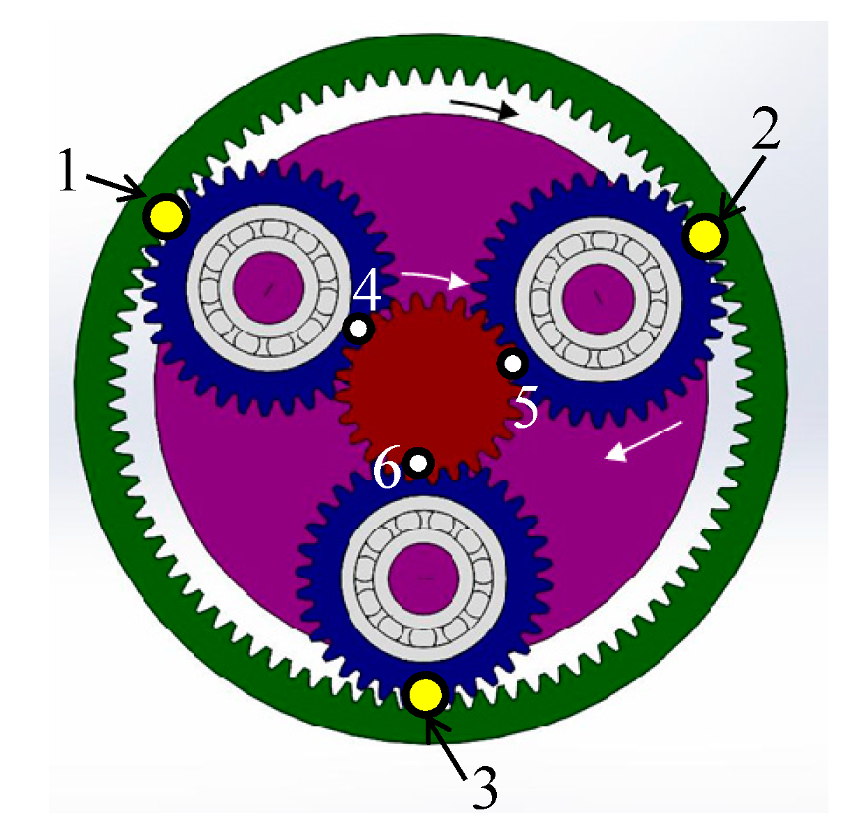
During the operation of a planetary gearbox, the planet carrier and sun gear rotate in the same direction. The planet gear and the sun gear mesh with each other, whilst the planet gears orbit around their own rotation axis and the planet carrier, as shown in Figure 1. It is assumed that the rotation direction of planet carrier is positive and its rotational frequency is , the planetary gear rotational frequency is , the absolute rotation frequency of planet gear is . The gear ring is connected with the case and it rotates with respect to the planet carrier at the frequency . The meshing frequency of planetary gearbox is:
wherein is the meshing frequency of planetary gearbox; is the number of gear ring tooth; is the number of sun gear tooth; is the number of planet gear tooth; is the rotational frequency of sun gear.
Taking a fixed point on the housing as reference point, the rotational frequency of planetary gear inner ring is equal to the planetary carrier’s, that is . The rotational frequency of planetary gear outer ring relative to the reference point is the absolute rotational frequency of planetary gear, that is .
The rotational frequency of planet gear bearing cage relative to this reference point is:
The characteristic frequency of planet gear bearing outer ring is:
The characteristic frequency of planet gear bearing inner ring is:
wherein, is the number of rolling elements, is the roller diameter, is the bearing pitch diameter, is the contact angle. is the rotational frequency of bearing cage. and represent the characteristic frequencies of planet gear bearing outer ring and planet gear bearing inner ring.
2.2. Fault Simulation Model
During the operation of planetary gearbox, the meshing points are shown as points 1 to 6 in Figure 1. In order to analyze the fault mechanism, the vibration signal model is established in the case of sensors are installed on the housing. In the paper, only time-varying transmission paths are considered, that is shown in Figure 2. The positions of all planetary gears are constantly changing during the operation. The transmission path of vibration signal generated by each meshing points to sensor is time-varying. Vibration transmission is mainly through these two paths. The first time-varying path starts from planet gear bearing to planet gear, and then to gear ring. Finally, it passes through the case to sensors. The second path has one more transmission of sun gear to planet gear than the first one, and its transmission length does not change with the rotation of planet carrier. Therefore, the second path is an equal-proportional attenuation process relative to the first one. Assuming that the amplitude modulation effect produced by the first path is , and then the amplitude modulation effect produced by the second path can be expressed as , where .
2.1.1. Amplitude Modulation Model
As the planetary gear moves from the bottom to the top of gearbox housing, it comes closer to the sensor and the impact characteristic strength of vibration signals collected by the sensor show an increasing trend. As the planetary gear moves from the top to the bottom of gearbox housing, the planetary gears are farther away from the sensor, and the vibration signals collected by the sensor are weaker. The amplitude modulation effect can be expressed as the following equation:
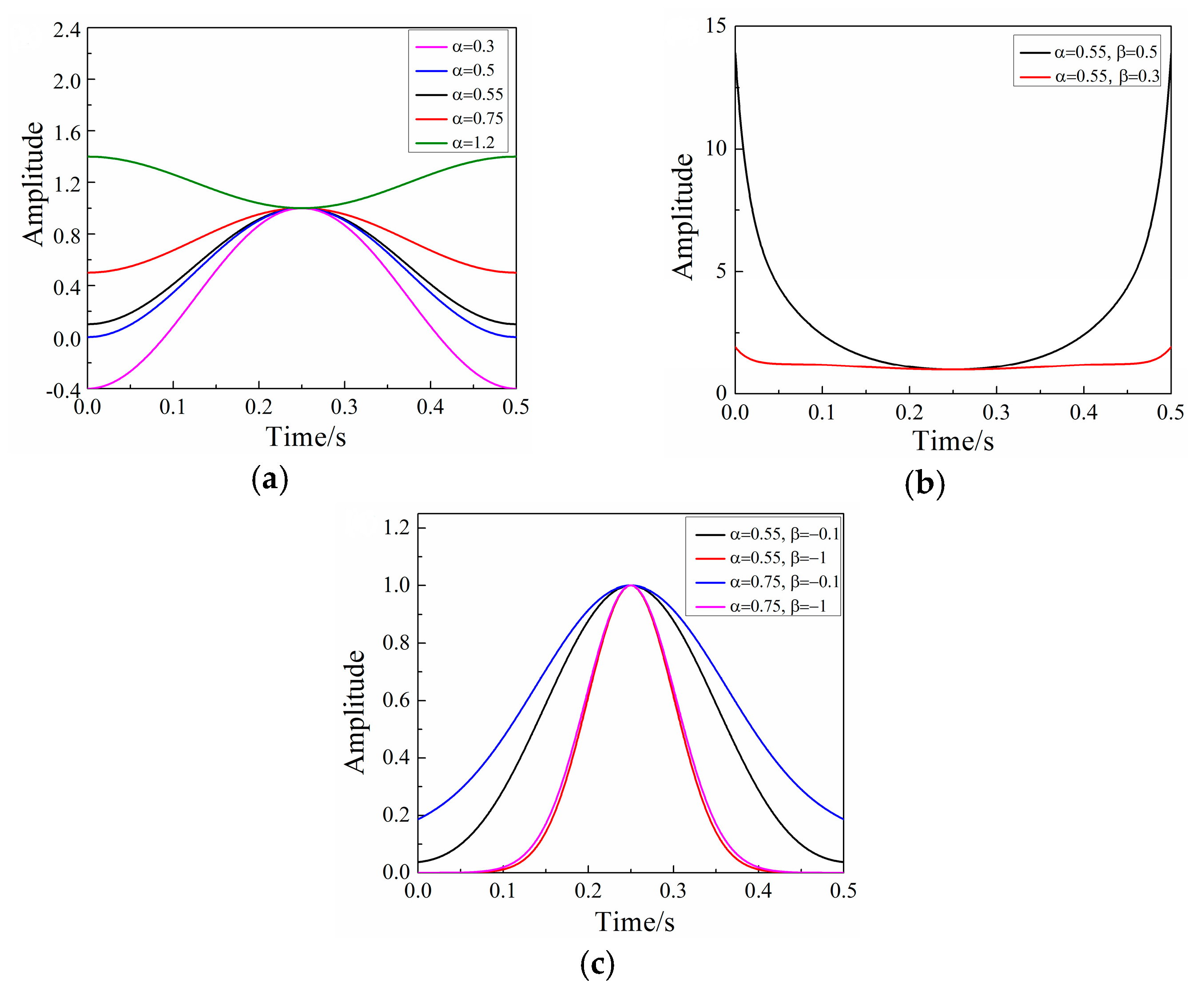
wherein, represents the amplitude modulation effect of planetary gearbox during operation. α and β indicate the intensity of modulation effect. is the phase difference between the planet gear and the first planet gear. The different modulation effects caused by different values of α and β are shown in Figure 3.
In Figure 3a, in the case of , all of the amplitudes are greater than 1. If , the amplitudes are less than 0. Neither of these two conditions satisfies the requirements. Therefore, it can be determined that is in the range of [0.5, 1]. In Figure 3b, when is fixed and , the amplitudes are greater than 1. The larger the value of , the greater the effect of amplification. When and , all of the amplitude concentrated between [0, 1], that meets the requirements.
2.2.2. Meshing Force Model
2.2.3. Fault Step-Impact Model
In the case where a bearing outer ring is cracked or peeled off, its geometry will change. As shown in Figure 4, when the rolling element is in contact with the fault position, the components of the vibration signal will change. Reference [31] proposed that the bearing fault signal is composed of two parts. A step signal will be generated when the rolling element enters the fault position and an impact signal will be generated when the rolling element leaves the fault position. The fault size can be quantified based on the time difference between the step signal and the impact signal. In this paper, the research mainly focuses on bearing faults occurred at an early stage, that is the case of a small fault size. The rolling element does not come into contact with the lowest end of the bearing outer ring fault when it passes through the fault area. It is assumed that the frequency of bearing cage is , the outer ring fault width is and is the outer ring diameter. Therefore, the time difference between the rolling element entering and leaving the fault area is:
The step response model can be expressed as:
The impact signal model can be expressed as:
The bearing failure vibration signal model:
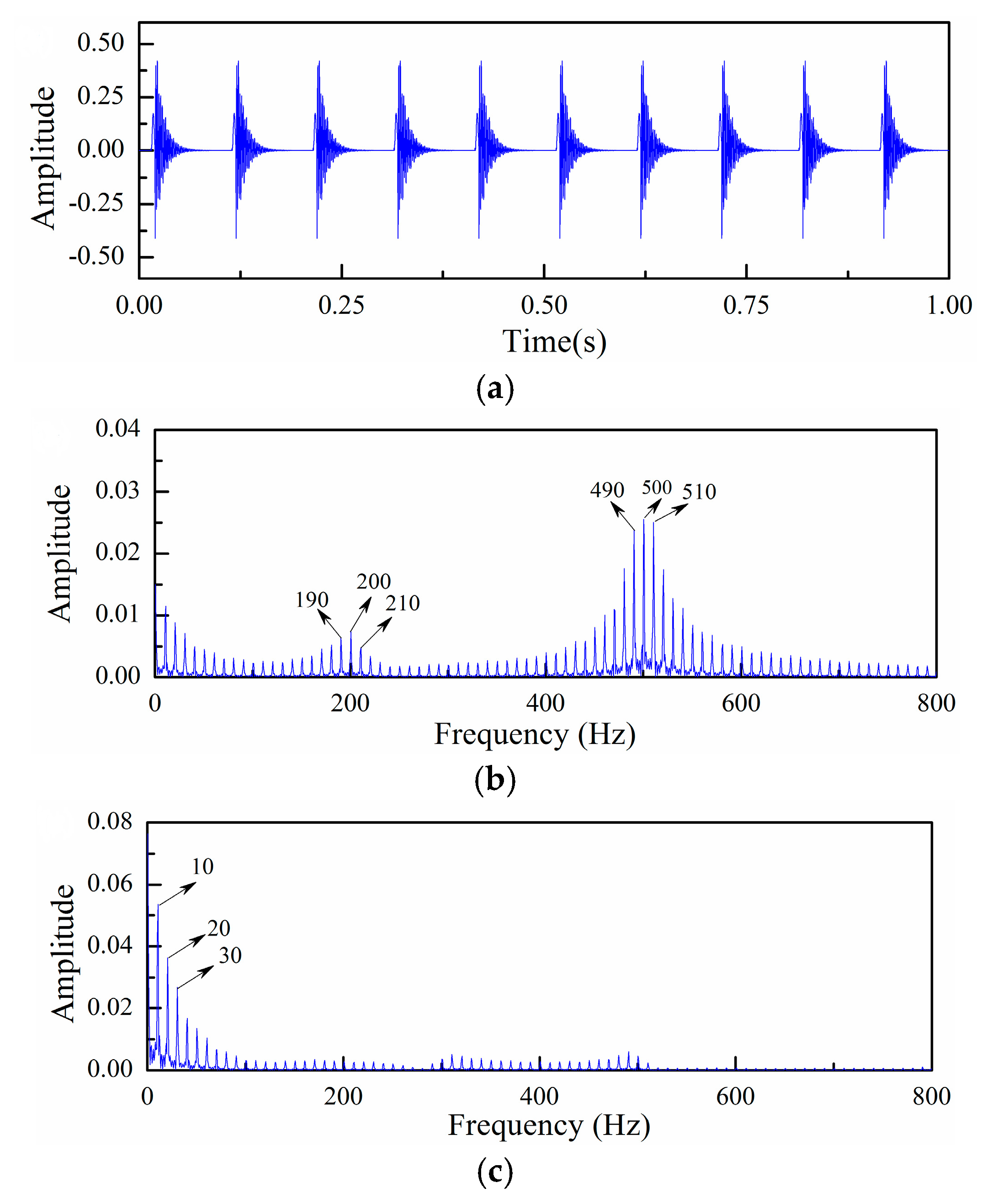
wherein, is the attenuation coefficient, and are the contributions of the above two vibration signal models. The step signal, impact signal, and bearing fault simulation model for a rotating cycle are shown in Figure 5a–c, respectively.
The simulated signal is determined as , , . The multi-cycle time domain waveform of bearing attenuation impact signal is shown in Figure 6a. In Figure 6b, the frequency spectrum analysis is continued, and the carrier frequencies of 500 Hz and 200 Hz are the center frequencies with the impact characteristic frequency 10 Hz and its multiplication frequency component is the side frequency spread over the entire frequency axis. In the envelope spectrum, only the impact characteristic frequency is demodulated.
2.2.4. Bearing Load Zone Pass Effect
During the operation of planetary gearbox, bearing capacity can be considered as the radial force along the radial direction. In the case of the rotation frequency of bearing outer ring is , the angle deviating from the vertical centerline is . The function expression of its load over time is:
wherein, is the maximum load density; is the load distribution factor; is the maximum angle of load distribution area. In the process of bearing rotation, there is not always load distribution in one period. The load will be zero when the rotation angle exceeds the maximum load distribution area. The maximum angle of load distribution area can be controlled by changing the size of . In addition, the magnitude of modulated vibration signal by load distribution is changed by resizing the maximum load density.
Assuming (n is the sampling length), , . In the case of , the signal model is shown in Figure 7. As can be seen from figure, meets the requirements.
2.2.5. Outer Ring Fault Vibration Signal Model
The vibration signal model of planet gear bearing outer ring fault is established based on the above analysis. In the process of modeling, bearing load zone passing effect, step-impact signal model, and the effect of transmission paths are all taken into account. Considering only one planet gear bearing outer ring failed, the vibration signal model is shown as follows:
wherein,
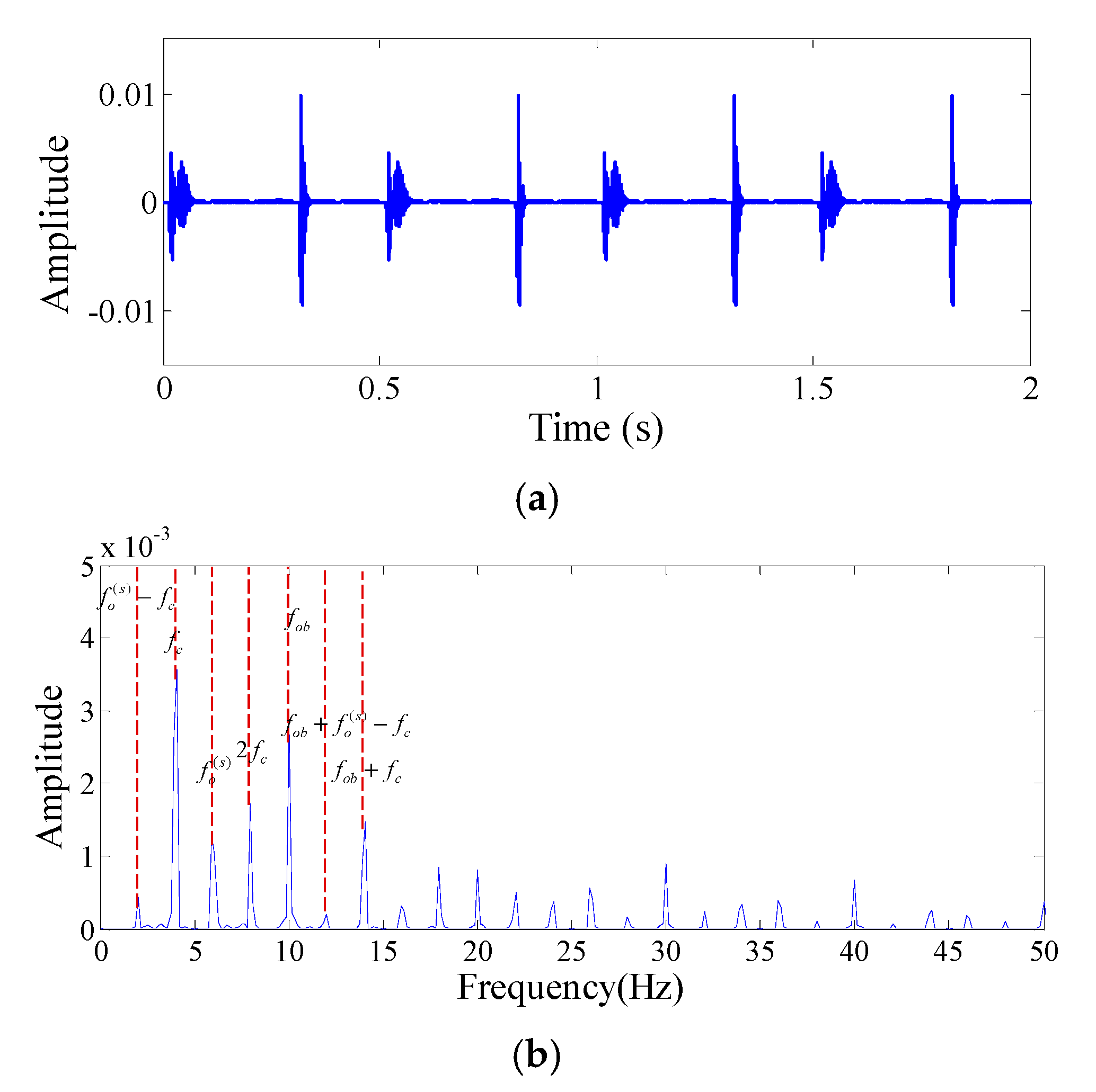
, , , , , , , . The repeat period of impact simulation signal is 100 ms. The time domain and frequency domain waveforms of simulated signal are shown in Figure 8.
By analyzing the time domain waveform and frequency spectrum of the planet gear bearing outer fault simulation signal, it can be seen that a series of impact signals are generated in the time domain signal when the bearing fails. The load of the bearing is changed due to the rotation of the planet gear bearing outer ring, thereby causing an intermittent distribution of the impact signal. The natural frequency of the bearing and its side frequency components appear in the envelope spectrum. In addition, there are side frequency components that are the characteristic frequency of bearing, carrier frequency and bearing rotation frequency. In summary, when the outer ring of planetary bearing fails, the frequency peak mainly appears in (, , are positive integers).
3. Theory of Proposed Method
3.1. Improved Wavelet Scalogram
As a method of time-frequency analysis, wavelet transform is adaptive. It can eliminate noise and identify weak fault information. The different scale value corresponds to different frequency band [32]. Select the appropriate scale value according to the frequency characteristics of the signal being analyzed. Suppose is a wavelet basis function, then it must satisfy finite energy theorem, i.e., and its Fourier transform should respect the following rule:
wherein is a wavelet basic function, also called mother wavelet. In general, the signal analysis results depend on the . Reference [33] discussed the effect of different mother wavelets on the analysis result of bearing impact failure signal. It is verified that the Morlet wavelet can better match the characteristic of bearing impact faults. Therefore, with a Morlet wavelet as mother wavelet to perform wavelet transform in the following section, a series of wavelet functions can be obtained by translating and stretching the mother wavelet . Taking as its scale factor and as the translation factor, the deformation of a basic wavelet function can be obtained by changing the values of and according to the following Equation (17):
is not unique, and its shape and position vary in relation to the values of and . The continuous wavelet transform was carried out on , that can be expressed in the general form of Equation (18):
wherein, is an analytical wavelet, is the complex conjugate of . This definition is analogous to the Fourier transform. What makes them different is the basis function: a Fourier transform is performed on cosine functions and wavelet transform depends on the wavelet function. The wavelet transform is reversible and the original signal can be restored by using the wavelet transform coefficients:
wherein can be defined as the modulus of continuous wavelet transform coefficients, which is given by Equation (20).
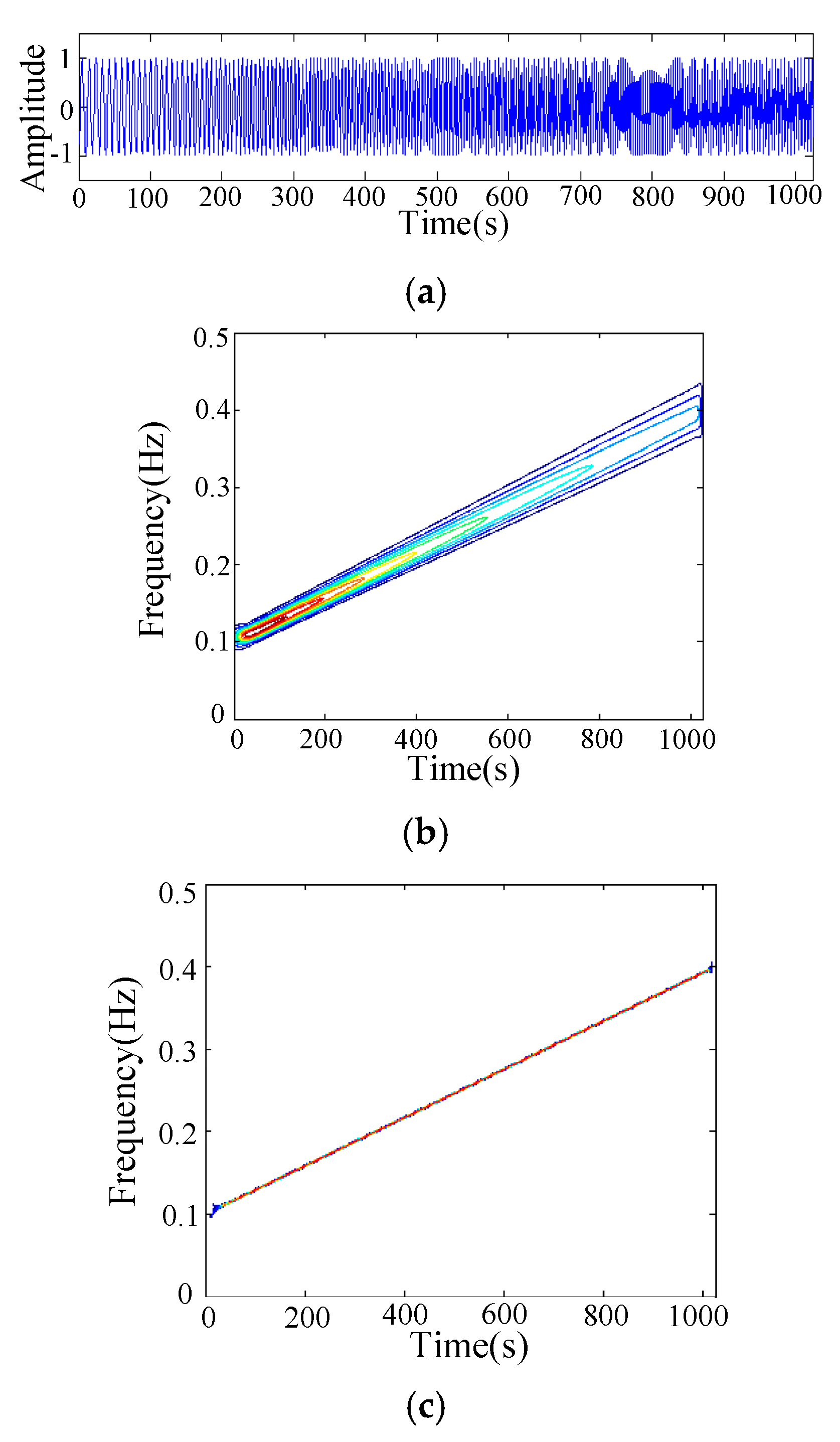
As mentioned earlier, a wavelet scalogram lacks concentricity just like other traditional time-frequency analysis method. Taking a simple chirp signal as an example, its time domain waveform is shown in Figure 9a, its time-frequency spectra obtained by a wavelet scalogram is shown in Figure 9b. It can be seen that the time-frequency ridge spreads over a wide area. Applying the reassigned wavelet scalogram to calculate the time-frequency ridge and the result is shown in Figure 9c. The picture displays that the time-frequency feature concentrated in a fine straight line.
Given the problem that the time-frequency resolution of wavelet scalogram is low, a reassigned method was put forward. The theoretical definition of improved wavelet scalogram is expressed as:
wherein, , , and can be calculated by the following equations:
wherein, is the central angular frequency. represents the average of the energy density of a region which takes as geometric center. Due to the fact the energy of this region is not geometrically symmetric and it is unreasonable to concentrate the average energy at the geometric center, at this time, some people advise placing the average energy at the local energy center . Then, a reassigned wavelet scalogram is put forward based on this principle.
For a detailed description about reassigned wavelet scalograms readers can consult [30]. In Figure 9c is easier to identify how the frequency changes with time compared with Figure 9b. The reassigned wavelet scalogram is a spectrogram that can improve readability after the average value is concentrated at the local energy center. The mechanical vibration signal generally exhibits a periodic characteristic, and its cycle is variable with the change of device operating state. Moreover, the operation of equipment is vulnerable to external interferences. Therefore, vibration signals collected from rotating machinery are often mixed with external interference that is independent of fault information. The fault feature is weak when the external interference is strong [16,17]. The traditional time domain and frequency domain analysis method is unable to diagnose weak faults. Then, a series of new methods are exploited to improve the accuracy of the fault diagnosis, such as the synchronous averaging technique [19,34].
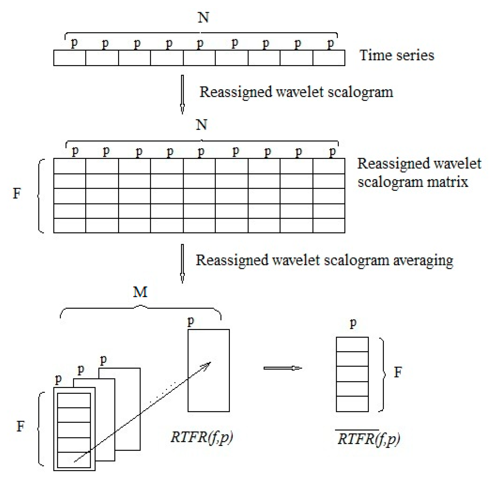
Let us suppose is a periodic vibration signal that was collected by a transducer mounted on a rotary machine, and its sampling point is , where . If the vibration signal is formed by stationary components with the period is , then . We choose the Morlet wavelet as the basic wavelet to perform wavelet transform on . After that, we can implement the reassignment process to obtain the reassigned wavelet scalogram according to Equation (21), where represents the frequency and represents the time. If the signal contains frequencies, then the size of is .
Based on the reassigned wavelet scalogram, we can use time synchronous averaging for further analysis. Each row corresponds to a frequency value, which is made up of repeating components with a period . An average for each cycle and time synchronous can be obtained.
The process diagram of the improved wavelet scalogram is displayed in Figure 10.
The value of directly affects the synchronous averaging results. The characteristic frequency is related to the running speed of the rolling element bearings. However, in some cases, they are not integer multiple relationships, so a one-step rounding process is usually added.
We can intercept the impact series to calculate the average points per cycle. In normal circumstances, we can select a proper signal length according to the signal characteristics for analysis in order to improve the computational efficiency, whilst not affecting the analysis results. The computational efficiency of Equation (26) will be low in the case where is large. In addition, the calculation accuracy will decrease in the case where is small. Therefore, when defining the value of , the calculation accuracy and computational complexity should both be taken into account.
3.2. Wavelet Ridge
The wavelet ridge [35] is a sequence points extracted from the maximum of modulus values of wavelet coefficients of time-frequency spectra at each moment. By analyzing the wavelet ridge, we can explore the composition of signal components, like signal envelope, instantaneous amplitude, and instantaneous phase. Suppose is a simple cosine signal. It can be expressed as and its analytic signal can be calculated by the following expression.
wherein, is the Hilbert transform of . is the instantaneous amplitude and is the instantaneous phase angle. The complex form of the mother wavelet is denoted as Equation (28).
Select as the wavelet basis for wavelet transform to analyze signal .
wherein, is the conjugate of .
The Morlet wavelet is selected as the basis function to match the vibration signal. That is determined by its downhill feature in a short time. This is very similarity to the bearing fault impulse signal. The expression of a Morlet complex wavelet is:
wherein, is the frequency band range and is wavelet center frequency. There is a one-to-one correspondence between wavelet transform scale and frequency. Suppose sampling frequency is and the corresponding frequency of scale is:
After obtaining the wavelet ridge line, the wavelet coefficients corresponding to wavelet ridge line position can be deduced by inverse transform formula [28,36].
is the modification item, which is usually small and often can be ignored. is the Fourier transform of , will reach maximum at the point of center frequency . With a slight modification for Equation (33), the amplitude of continuous wavelet transform is approximately equal to:
In wavelet function expression, the parameter b represents time shift. Then, can be taken as . Accordingly, can be represented as . In this circumstance, the instantaneous amplitudes of signal envelope are estimated by:
In the same way, Equation (20) can be transformed into Equation (36).
Afterwards, instantaneous amplitudes of signals can be approximated by Equation (37).
It can be seen from Equation (37) that the wavelet ridge extraction process is actually a demodulation process. In the same way, the instantaneous amplitudes of signal can be estimated on the improved wavelet scalogram according to Equation (37). There are two different ways to extract wavelet ridge. The one way is based on wavelet coefficient phase values and the other one is based on modulus values. By comparing both analysis results, it can be concluded that the method on the basis of wavelet coefficient modulus is more accurate. Because the local maximum value of the wavelet scale spectral coefficients and the continuous wavelet transform coefficients is the same point that is the wavelet ridge point [28]. In this paper, the wavelet ridge is extracted by calculating the wavelet coefficient modulus maximum and a new time series was reconstructed. Reference [37] proposed a method to extract the wavelet ridge which minimizes the cost function. This method only needs the model information to extract the ridge line. There are cost functions along the wavelet ridge line described in the following equation.
The ridge point can be determined according to the Equation (38). If the ridge point was derived, then the ridge point can be determined by minimizing the . During run time, each choice is evaluated in order. When all of the items (from to ) are completely calculated, the instantaneous amplitudes of the signal can be estimated according to Equation (37). Due to the bearing fault signal presents periodic impact characteristics, which can be identified from the instantaneous amplitude. In general, a small scale band is chosen for analysis, thereby improving the accuracy of wavelet ridge extraction results.
It is indicated that 3 dB bandwidth is the most suitable choice according to the characteristic of signal being analyzed. The region where the wavelet coefficients modulus is large usually corresponds to the range of the wavelet ridge. Besides, selecting a suitably small scale to analyze can reduce the calculation time.
3.3. Incipient Feature Extraction Method
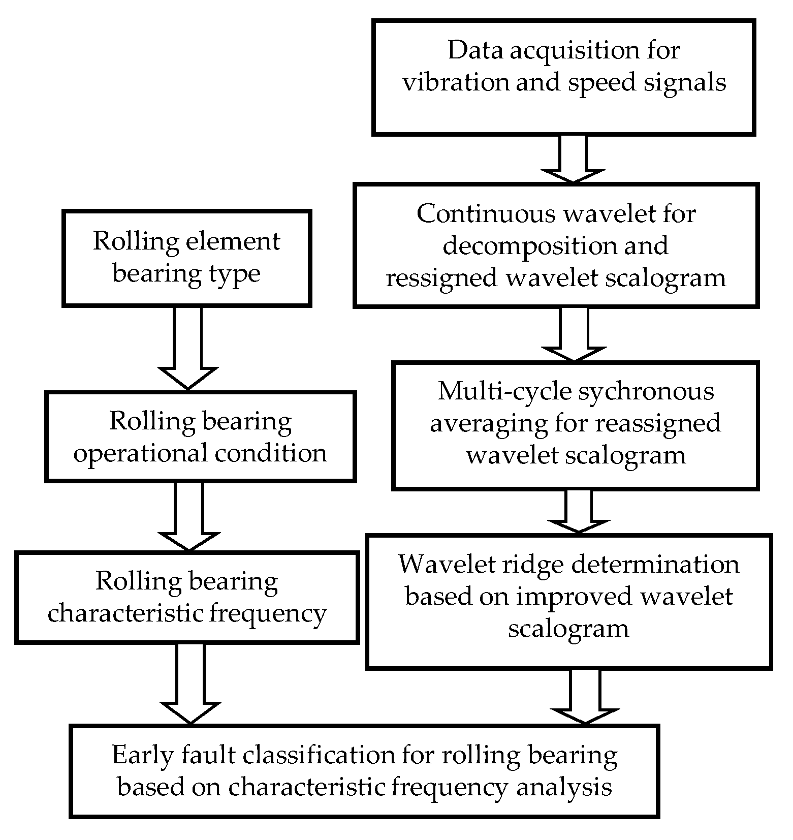
The process flow diagram of rolling element bearing fault diagnosis based on improving wavelet scalogram and wavelet ridge is shown in Figure 11. This method is readily available for rolling element bearing fault feature extraction. To begin with, the improved wavelet scalogram plays an important role in extracting and enhancing the impact characteristics. In addition to that, the wavelet ridge can identify fault frequency more clearly. This method does not require any prior knowledge of rolling element bearing fault information, and can be applied to determine the weak fault characteristics for rolling element bearings.
4. Algorithm Verification
4.1. Simulation Analysis
In order to prove the validity of the wavelet ridge line method based on improved wavelet scalogram, the simulation signal that is established by researching the characteristics of rolling element bearing taken as an analytical object. We add Gaussian white noise with a signal-to-noise ratio size of −15 dB into the planet gear bearing outer ring fault signal simulation model which is shown in Figure 8a. The time-domain impact characteristic signal is almost invisible in Figure 12, which can represent as a weak impact signal.
Subsequently, the envelope spectrum is applied on the noise-added simulation signal. It can be seen that the envelope analysis is infeasible for weak impact feature extraction. Then, a wavelet transform is further performed on it. Its reassigned wavelet scalogram was calculated as shown in Figure 13. Many spectral lines are scattereded in the wavelet scalogram spectrum. It is difficult to recognize the impact information by adopting the reassigned wavelet scalogram method under the situation of strong noise. There are many interfering components in the spectrum because of outside noise. In order to eliminate more irrelevant interference information, the scalogram is further processed by synchronous averaging where the synchronous cycle is 400 ms. The improved wavelet scalogram of the noisy simulation signal is shown in Figure 14. The impact characteristics from the time-frequency spectrum can be easily distinguished. All of the impact components in the simulation signal are concentrated in the frequency axis of 500 Hz. The time interval between the two impact positions is 100 ms. That is to say that the impact period is 100 ms and the impact characteristic frequency is 10 Hz. This is consistent with the theoretical value of the simulation signal.
Although it can be seen that the wavelet scale spectrum has a periodic distribution characteristic in Figure 14, the impact information is distributed in an area of the block rather than a point or a line. The fault period cannot be extracted from Figure 14 correctly using the synchronous averaging scalogram. There is a lack of intuition and veracity. In this paper, further analysis is performed by using the wavelet ridge extraction method. The analysis scale area is limited to between 6 and 29 in terms of the characteristic frequency range obtained by the computational equation of wavelet ridge. The wavelet ridge extracted from Figure 14 is shown in Figure 15. Then, the instantaneous amplitude and the corresponding frequency can be calculated according to Equation (37) and the Fourier transform, as shown in Figure 16a,b. The impact characteristic frequency 10 Hz and its multiplied frequency components are clearly displayed in Figure 16b.
When the signal is disturbed by strong background noise, fault information cannot be separated from the time domain waveform directly. The weak impact characteristics of the noisy simulation signal were clearly and exactly extracted by adopting the improved wavelet scalogram algorithm which is proposed in this paper. The reassigned wavelet scalogram was used to enhance impact features firstly. Then, the outside interference components were decreased after synchronous averaging is performed on the reassigned wavelet scalogram. Finally, the visibility and the accuracy of time-frequency spectrum were improved by extracting the wavelet ridge. The wavelet coefficients characterize the similarity between the signal being analyzed and the basic wavelet. The larger the wavelet coefficients, the stronger the impact characteristic of the signal and the more obvious the fault feature. The modulus of wavelet coefficients of every frequency points at each moment can be highlighted by extracting the wavelet ridge on improved wavelet scalogram. By further analysis of the wavelet ridge, it is easily to extract the time domain and frequency domain information of fault impulses. By analyzing the simulation signals, it can be concluded that the proposed method is suitable for detecting the weak impact features.
4.2. Experimental Study
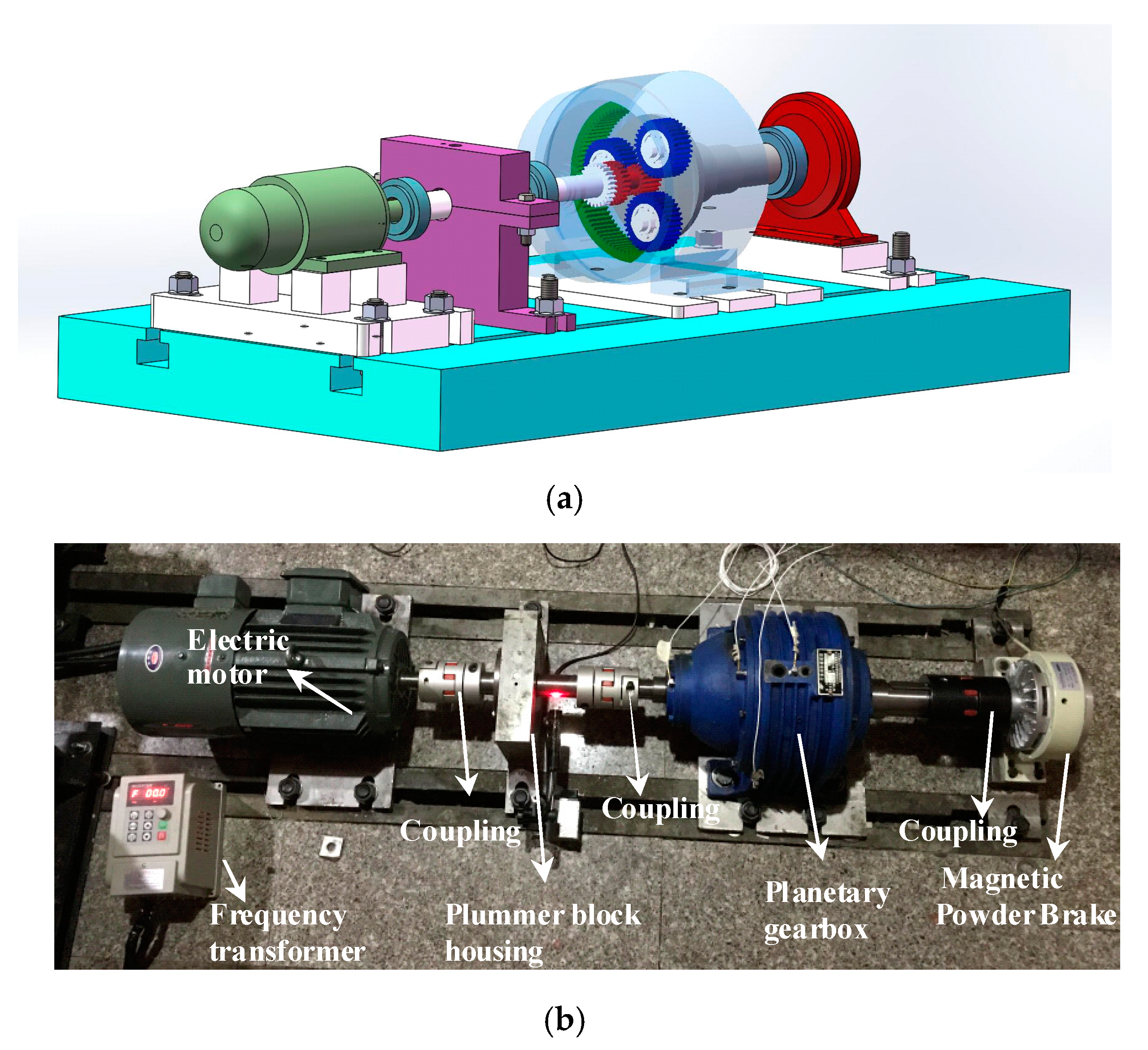
In order to further demonstrate the validity of the method presented in this research, signals were collected from a planet gear rolling element bearing experiment rig for analysis. The schematic diagram of the bearing test-to-failure experiment system is shown in Figure 17. On the laboratory bench, a frequency transformer drives one motor connected to the bearing housing, the planetary gearbox and the magnetic powder brake through the coupling. The planet gear bearing outer ring is machined with a 1 mm wide fault and the bearing surface structure after machining failure is shown in Figure 18. Planetary gearbox parameters are shown in Table 1. After calculation, the parameters of each component during operation are shown in Table 2.
In the event of a failure in the outer ring of planet gear, the fault characteristics of the original acceleration signal measured by sensors are weak because of the long and complex transmission path between the vibration source and measuring points. There is no impact characteristic in its time domain waveform as shown in Figure 19a. Only the rotation frequency component of the shaft and its differential frequency components with the planetary carrier exist in Figure 19b. The fault characteristic frequency cannot be determined from the frequency domain waveform.
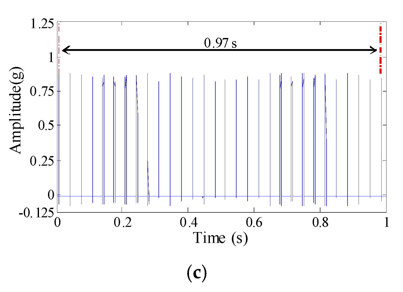
It can be concluded that the traditional spectral analysis method is inapplicable for planetary bearing fault diagnosis. According to the key phase signal shown in Figure 19c, the sun gear rotation frequency of the planetary gearbox is approximately 29.7 Hz. Defining a value of 127 ms as the synchronization cycle, afterward, a continuous wavelet transform was carried out on the planet bearing outer ring vibration signals. Twenty synchronization period signals were selected for analysis. The wavelet scalogram and improved wavelet scalogram results are displayed in Figure 20a,b, respectively.
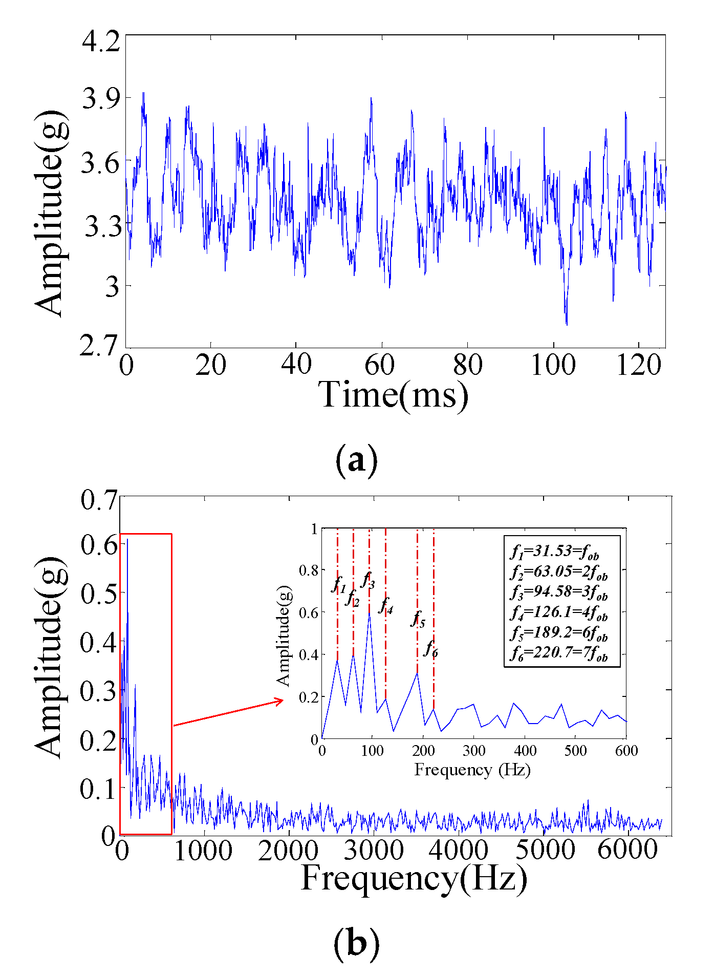
The wavelet ridges extracted from the improved wavelet scalogram are shown in Figure 21. The instantaneous amplitude and the corresponding frequency were calculated according to Equation (37) and the Fourier transform formula, as shown in Figure 22. It can be observed that the planet bearing outer ring fault characteristic frequency is 31.53 Hz and its multiplied frequency components are clearly displayed in the partial enlarged view in the upper right corner of Figure 22b. For planet gear bearing fault signals with weak impact characteristics, the fault features cannot be directly extracted by envelope spectrum analysis. Fortunately, the interference information is weakened by using the improved wavelet scalogram analysis. This method is very effective for enhancing the impact characteristics. Subsequently, wavelet ridge extraction is also considered as an improved envelope extraction method and the faint fault information under external interference is extracted by a series of transforms. The above description indicates that the proposed method has a better performance in planet gear bearing weak fault diagnosis. Based on the above simulation signal and vibration signal analysis, it can be concluded that the proposed method is effective for rolling element bearing analysis.
5. Conclusions
A vibration signal model is established by studying the vibration mechanism of planetary gearboxes, which is the theoretical basis of diagnosing the running state of planetary bearings based on the vibration signal analysis method. In addition, bearing fault signal weak impact feature determination is very difficult because of the excessive interference. This paper applied synchronous averaging to reduce the disturbed components of a reassigned wavelet scalogram which is obtained by multi-scale analysis of a continuous wavelet transformation, thus improving the wavelet time-frequency resolution. As well, a wavelet ridge is extracted to improve the visibility and the accuracy of the time-frequency spectrum. The results indicated that the newly proposed method has good performance in detecting of planet gear bearing weak fault signals that are usually masked by external disturbances. This method can contribute to weak impact characteristic determination in bearing fault analysis.
Author Contributions
R.Y. built the simulation model, analyzed the data and wrote the paper; H.L. conceived the signal processing method and guided the writing of paper; C.W. and C.H. designed the test stand and the experiments.
Acknowledgments
This research was funded by Chinese National Science Foundation (No. 51575075) and Chinese National Science Foundation (No. 51175057), and Collaborative Innovation Center of Major Machine Manufacturing in Liaoning for this research is gratefully acknowledged.
Conflicts of Interest
The authors declare no conflict of interest.
References
- Lihovd, E.; Johannssen, T.I.; Steinebach, C.; Rasmussen, M. Intelligent diagnosis and maintenance management. J. Intell. Manuf. 1998, 9, 523–537. [Google Scholar] [CrossRef]
- Lei, Y.G.; Lin, J.; Zuo, M.J.; He, Z. Condition monitoring and fault diagnosis of planetary gearboxes: A review. Measurement 2013, 48, 292–305. [Google Scholar] [CrossRef]
- Mcfadden, P.D.; Smith, J.D. An Explanation for the Asymmetry of the Modulation Sidebands about the Tooth Meshing Frequency in Epicyclic Gear Vibration. Proc. Inst. Mech. Eng. Part C 1985, 199, 65–70. [Google Scholar] [CrossRef]
- Mosher, M. Understanding Vibration Spectra of Planetary Gear Systems for Fault Detection. In Proceedings of the ASME 2003 International Design Engineering Technical Conferences and Computers and Information in Engineering Conference, Chicago, IL, USA, 2–6 September 2003; pp. 645–652. [Google Scholar]
- Inalpolat, M.; Kahraman, A. A theoretical and experimental investigation of modulation sidebands of planetary gear sets. J. Sound Vib. 2009, 323, 677–696. [Google Scholar] [CrossRef]
- Inalpolat, M.; Kahraman, A. A dynamic model to predict modulation sidebands of a planetary gear set having manufacturing errors. J. Sound Vib. 2010, 329, 371–393. [Google Scholar] [CrossRef]
- Feng, Z.; Zuo, M.J. Vibration signal models for fault diagnosis of planetary gearboxes. J. Sound Vib. 2012, 331, 4919–4939. [Google Scholar] [CrossRef]
- Liang, X.; Zuo, M.J.; Hoseini, M.R. Vibration signal modeling of a planetary gear set for tooth crack detection. Eng. Fail. Anal. 2015, 48, 185–200. [Google Scholar] [CrossRef]
- Lei, Y.G.; Tang, W.; Kong, D.T. Vibration Signal Simulation and Fault Diagnosis of Planetary Gearboxes Based on Transmission Mechanism Analysis. J. Mech. Eng. 2014, 50, 61–68. [Google Scholar] [CrossRef]
- Huang, Y.H.; Ding, K.; He, G.L. Mathematical Model of Planetary Gear Sets’ Vibration Signal and Characteristic Frequency Analysis. J. Mech. Eng. 2016, 52, 46–53. [Google Scholar] [CrossRef]
- Antoni, J. The spectral kurtosis: A useful tool for characterising non-stationary signals. Mech. Syst. Signal Process. 2006, 20, 282–307. [Google Scholar] [CrossRef]
- Antoni, J. Fast computation of the kurtogram for the detection of transient faults. Mech. Syst. Signal Process. 2007, 21, 108–124. [Google Scholar] [CrossRef]
- Lei, Y.G.; Lin, J.; He, Z.J.; Zi, Y.Y. Application of an improved kurtogram method for fault diagnosis of rolling element bearings. Mech. Syst. Signal Process. 2011, 25, 1738–1749. [Google Scholar] [CrossRef]
- Wang, Y.X.; Liang, M. An adaptive SK technique and its application for fault detection of rolling element bearings. Mech. Syst. Signal Process. 2011, 25, 1750–1764. [Google Scholar] [CrossRef]
- Chen, X.; Feng, F.; Zhang, B. Weak Fault Feature Extraction of Rolling Bearings Based on an Improved Kurtogram. Sensors 2016, 16, 1482. [Google Scholar] [CrossRef] [PubMed]
- Antoni, J.; Daniere, J.; Guillet, F. Effective vibration analysis of IC engines using cyclostationarity. Part I—A methodology for condition monitoring. J. Sound Vib. 2002, 257, 815–837. [Google Scholar] [CrossRef]
- Antoni, J.; Daniere, J.; Guillet, F.; Randall, R.B. Effective vibration analysis of IC engines using cyclostationarity. Part II—New results on the reconstruction of the cylinder pressures. J. Sound Vib. 2002, 257, 839–856. [Google Scholar] [CrossRef]
- Do, V.T.; Le, C.N. Adaptive Empirical Mode Decomposition for Bearing Fault Detectionp. J. Mech. Eng. 2016, 62, 281–290. [Google Scholar] [CrossRef]
- McFadden, P.D.; Toozhy, M.M. Application of synchronous averaging to vibration monitoring of rolling element bearings. Mech. Syst. Signal Process. 2000, 14, 891–906. [Google Scholar] [CrossRef]
- Zhu, L.M.; Ding, H.; Zhu, X.Y. Synchronous averaging of time-frequency distribution with application to machine condition monitoring. J. Vib. Acoust. 2007, 129, 441–447. [Google Scholar] [CrossRef]
- Zhang, H.; Chen, X.; Du, Z.; Yan, R. Kurtosis based weighted sparse model with convex optimization technique for bearing fault diagnosis. Mech. Syst. Signal Process. 2016, 80, 349–376. [Google Scholar] [CrossRef]
- Ding, X.; He, Q. Time-frequency manifold sparse reconstruction: A novel method for bearing fault feature extraction. Mech. Syst. Signal Process. 2016, 80, 392–413. [Google Scholar] [CrossRef]
- Qian, Y.; Yan, R.; Hu, S. Bearing Degradation Evaluation Using Recurrence Quantification Analysis and Kalman Filter. IEEE Trans. Instrum. Meas. 2014, 63, 2599–2610. [Google Scholar] [CrossRef]
- Liu, J.; Wang, W.; Golnaraghi, F. An Extended Wavelet Spectrum for Bearing Fault Diagnostics. IEEE Trans. Instrum. Meas. 2008, 57, 2801–2812. [Google Scholar]
- Qin, Y.; Mao, Y.F.; Tang, B.P. Vibration signal component separation by iteratively using basis pursuit and its application in mechanical fault detection. J. Sound Vib. 2013, 332, 5217–5235. [Google Scholar] [CrossRef]
- Huang, N.E.; Shen, Z.; Long, S.R. The empirical mode decomposition and the Hilbert spectrum for nonlinear and non-stationary time series analysis. Proc. R. Soc. Lond. A 1998, 254, 903–995. [Google Scholar] [CrossRef]
- Soualhi, A.; Medjaher, K.; Zerhouni, N. Bearing Health Monitoring Based on Hilbert-Huang Transform, Support Vector Machine, and Regression. IEEE Trans. Instrum. Meas. 2015, 64, 52–62. [Google Scholar] [CrossRef]
- He, Q.B.; Wang, X.X. Time-frequency manifold correlation matching for periodic fault identification in rotating machines. J. Sound Vib. 2013, 332, 2611–2626. [Google Scholar] [CrossRef]
- Halim, E.B.; Choudhury, M.A.A.S.; Shah, S.L.; Zuo, M.J. Time domain averaging across all scales: A novel method for detection of gearbox faults. Mech. Syst. Signal Process. 2008, 22, 261–278. [Google Scholar] [CrossRef]
- Peng, Z.K.; Chu, F.L.; Tse, P.W. Detection of the rubbing-caused impacts for rotor-stator fault diagnosis using reassigned scalogram. Mech. Syst. Signal Process. 2005, 19, 391–409. [Google Scholar] [CrossRef]
- Sawalhi, N.; Randall, R.B. Vibration response of spalled rolling element bearings: Observations, simulations and signal processing techniques to track the spall size. Mech. Syst. Signal Process. 2011, 25, 846–870. [Google Scholar] [CrossRef]
- Peng, Z.K.; Chu, F.L. Application of the wavelet transform in machine condition monitoring and fault diagnostics: A review with bibliography. Mech. Syst. Signal Process. 2004, 18, 199–221. [Google Scholar] [CrossRef]
- Yan, R.; Gao, R.X. Impact of wavelet basis on vibration analysis for rolling bearing defect diagnosis. In Proceedings of the 2011 IEEE International Instrumentation and Measurement Technology Conference, Beijing, China, 10–12 May 2011; pp. 1–4. [Google Scholar]
- Siegel, D.; Al-Atat, H.; Shauche, V.; Liao, L.X.; Snyder, J.; Lee, J. Novel method for rolling element bearing health assessment—A tachometer-less synchronously averaged envelope feature extraction technique. Mech. Syst. Signal Process. 2012, 29, 362–376. [Google Scholar] [CrossRef]
- Qin, Y.; Tang, B.; Mao, Y. Adaptive signal decomposition based on wavelet ridge and its application. Signal Process. 2015, 120, 480–494. [Google Scholar] [CrossRef]
- Mallat, S. A Wavelet Tour of Signal Processing; China Machine Press: Beijing, China, 2003; pp. 67–81. [Google Scholar]
- Liu, H.; Cartwright, A.N.; Basaran, C. Moire interferogram phase extraction: A ridge detection algorithm for continuous wavelet transforms. Appl. Opt. 2004, 43, 850–857. [Google Scholar] [CrossRef] [PubMed]
Figure 1.
Planetary gearbox model diagram.

Figure 2.
Vibration signal transmission in planetary gearbox. 1. From planet gear to gear ring, to housing, then to sensors; 2. From sun gear to planet gear, to gear ring, to housing, then to sensors.
Figure 2.
Vibration signal transmission in planetary gearbox. 1. From planet gear to gear ring, to housing, then to sensors; 2. From sun gear to planet gear, to gear ring, to housing, then to sensors.
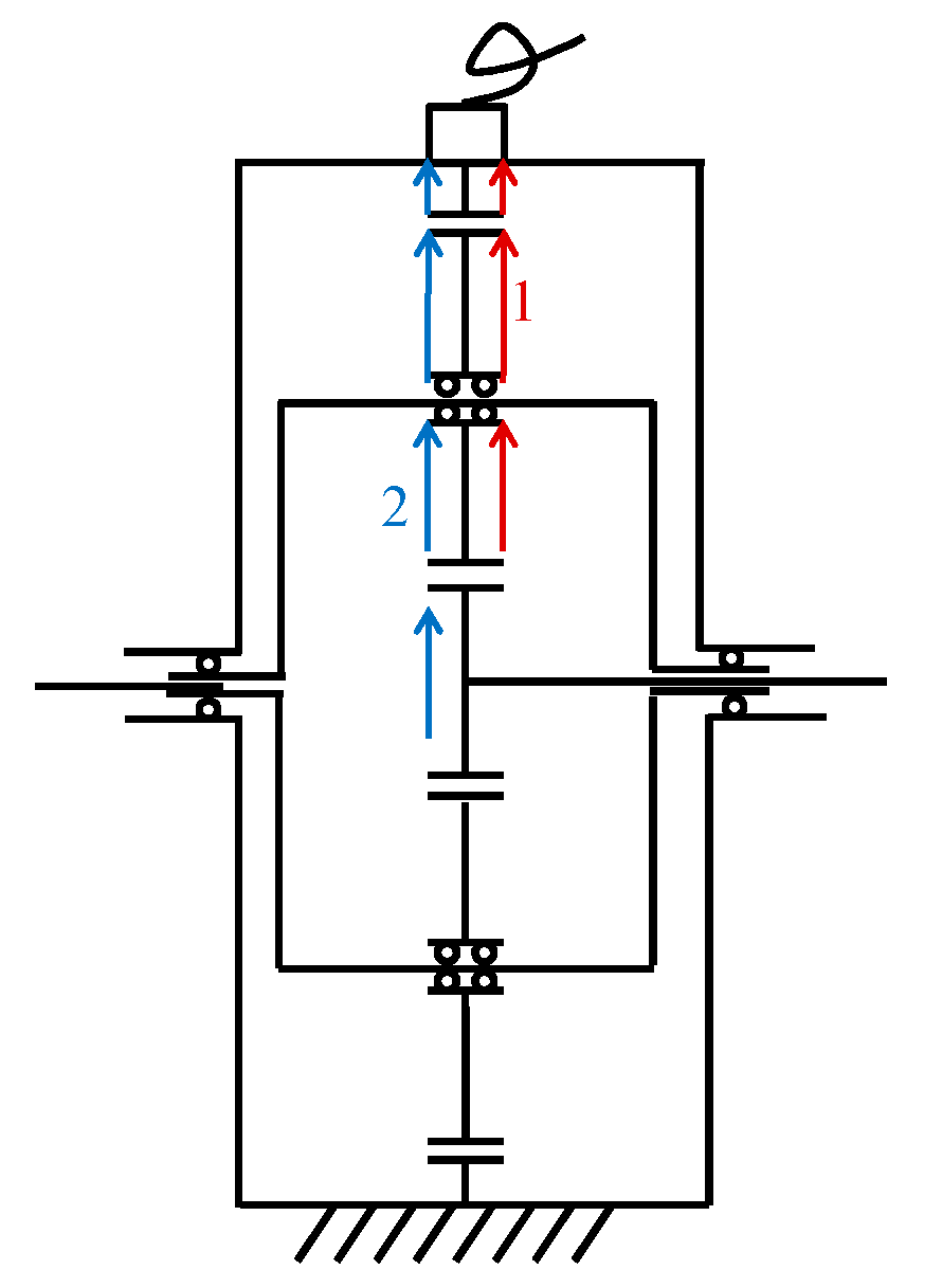
Figure 3.
The influence of different and values on exponential decay function; (a) The exponential decay effect of different values of ; (b) The exponential decay effect of different values of ; (c) The exponential decay effect of different values of and .
Figure 3.
The influence of different and values on exponential decay function; (a) The exponential decay effect of different values of ; (b) The exponential decay effect of different values of ; (c) The exponential decay effect of different values of and .

Figure 4.
Schematic diagram of rolling element fault position. (a) Schematic diagram of the rolling element entering the fault location; (b) Schematic diagram of the rolling element leaving the fault location.
Figure 4.
Schematic diagram of rolling element fault position. (a) Schematic diagram of the rolling element entering the fault location; (b) Schematic diagram of the rolling element leaving the fault location.
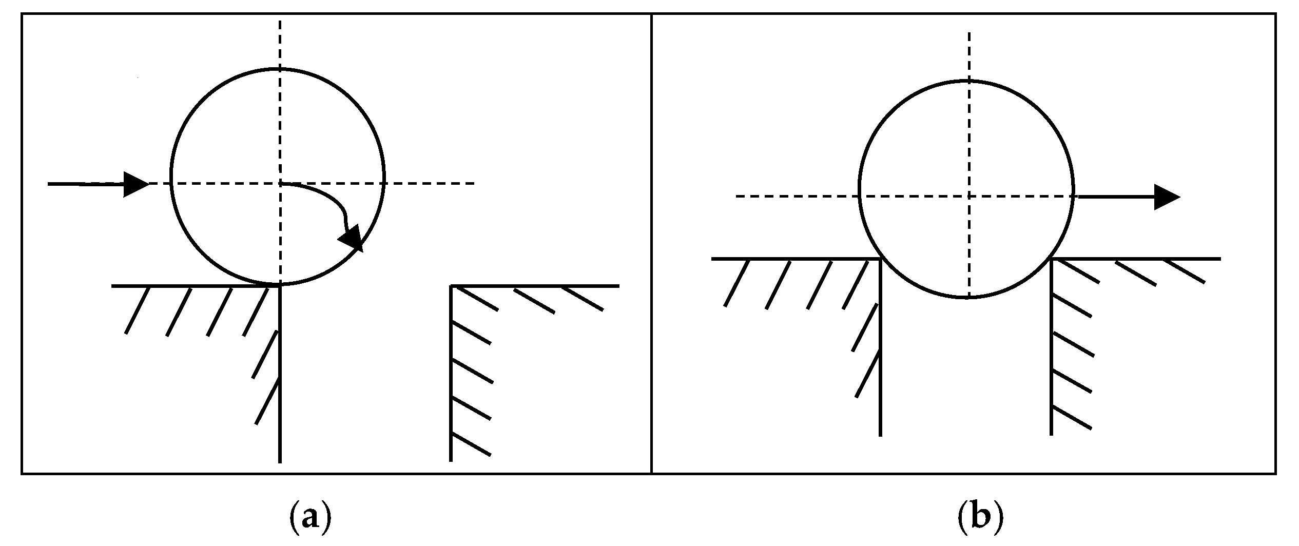
Figure 5.
Single-cycle bearing fault signal model. (a) The time domain waveform of step signal; (b) The time domain waveform of impact signal; (c) The time domain simulation waveform for quantitative analysis of bearing faults.
Figure 5.
Single-cycle bearing fault signal model. (a) The time domain waveform of step signal; (b) The time domain waveform of impact signal; (c) The time domain simulation waveform for quantitative analysis of bearing faults.
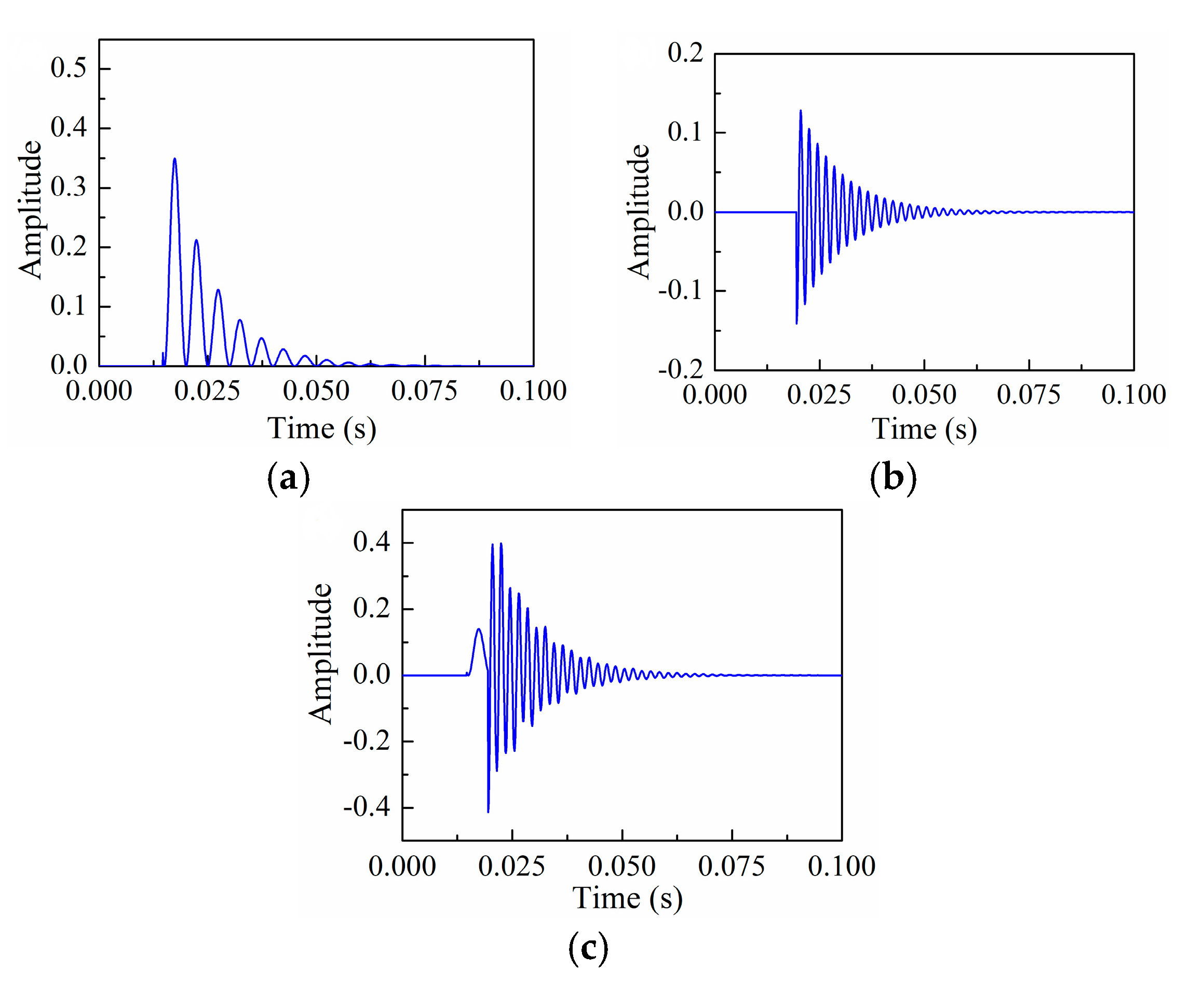
Figure 6.
The analytic results of bearing multi-cycle fault signal; (a) The time domain waveform; (b) The frequency domain waveform; (c) The envelope spectrum.
Figure 6.
The analytic results of bearing multi-cycle fault signal; (a) The time domain waveform; (b) The frequency domain waveform; (c) The envelope spectrum.

Figure 7.
The effect of load distribution factor on vibration waveform.

Figure 8.
The analytic results of planet gear bearing outer ring fault simulation signal. (a) Time domain waveform of simulation signal; (b) The envelope spectrum of simulation signal.
Figure 8.
The analytic results of planet gear bearing outer ring fault simulation signal. (a) Time domain waveform of simulation signal; (b) The envelope spectrum of simulation signal.

Figure 9.
Simulation signal analysis. (a) Time waveform for a line modulation signal; (b) Wavelet scalogram for the line modulation signal; (c) Reassigned wavelet scalogram.
Figure 9.
Simulation signal analysis. (a) Time waveform for a line modulation signal; (b) Wavelet scalogram for the line modulation signal; (c) Reassigned wavelet scalogram.

Figure 10.
Multi-scales synchronous averaging of reassigned wavelet scalogram.

Figure 11.
Flowchart for rolling element bearing fault diagnosis.

Figure 12.
The analytic results of simulation signal with Gaussian white noise. (a) The time domain waveform for noisy simulation signal; (b) The envelope spectrum for noisy simulation signal.
Figure 12.
The analytic results of simulation signal with Gaussian white noise. (a) The time domain waveform for noisy simulation signal; (b) The envelope spectrum for noisy simulation signal.
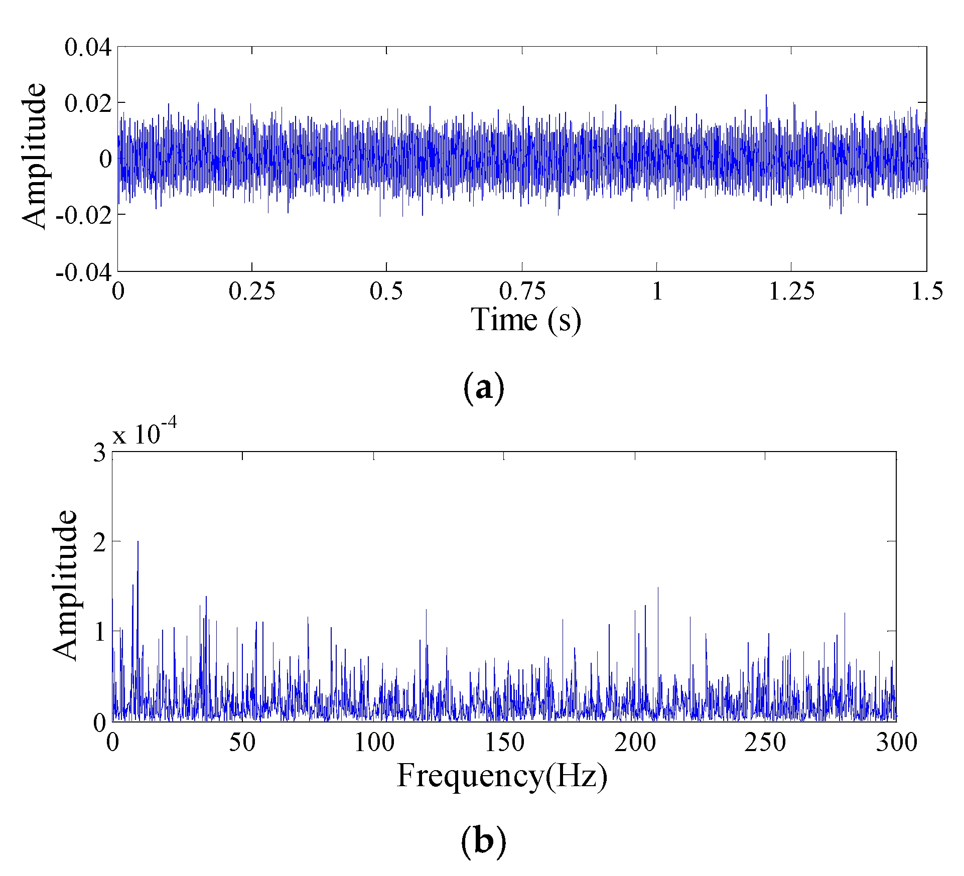
Figure 13.
Time frequency reassignment distribution for the simulation signal.
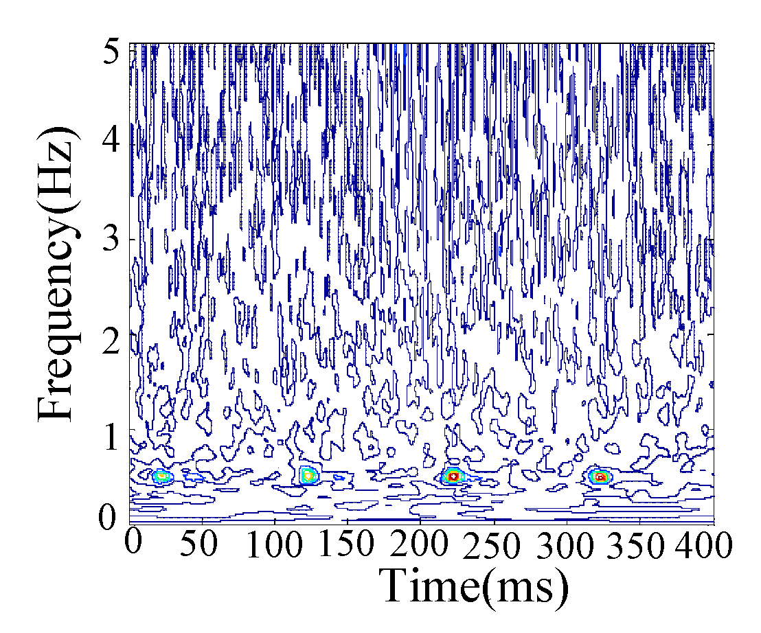
Figure 14.
The scalogram under synchronous averaged.
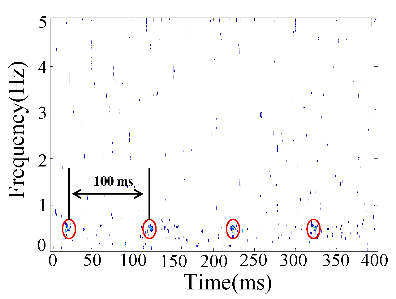
Figure 15.
Wavelet ridge for improved wavelet scalogram.
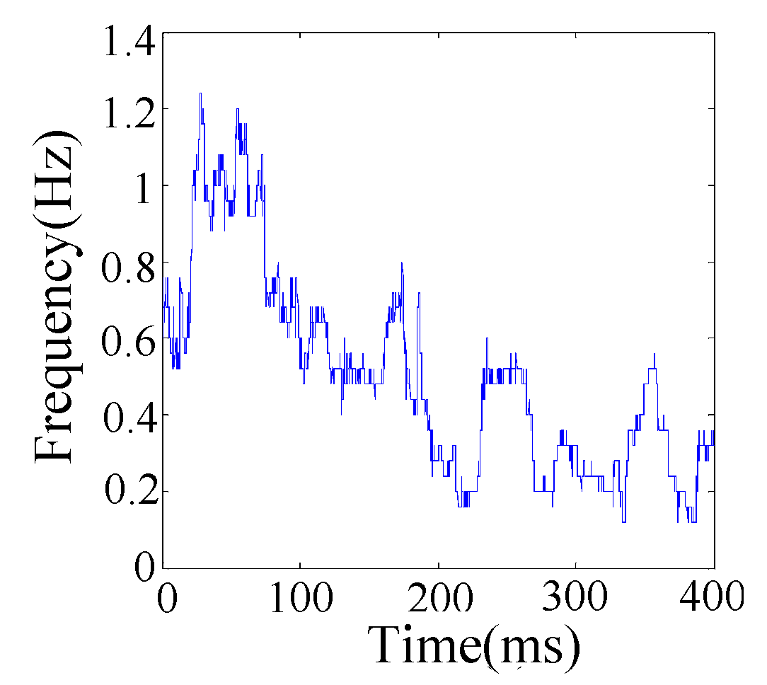
Figure 16.
The analytic results of simulation signal’s instantaneous amplitude. (a) Time-domain waveform of simulation signal’s instantaneous amplitude; (b) The frequency domain waveform of simulation signal’s instantaneous amplitude.
Figure 16.
The analytic results of simulation signal’s instantaneous amplitude. (a) Time-domain waveform of simulation signal’s instantaneous amplitude; (b) The frequency domain waveform of simulation signal’s instantaneous amplitude.
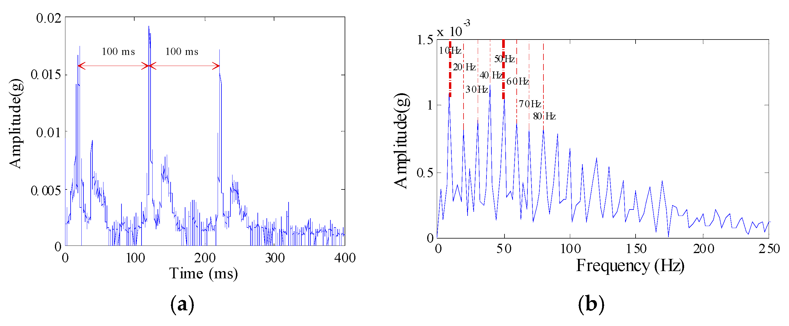
Figure 17.
A bearing test-to-failure experiment system. (a) System structure; (b) Test system.

Figure 18.
Planetary bearing outer ring fault surface map.

Figure 19.
The analytic results of planetary bearing outer ring fault. (a) The time domain waveform of planetary bearing outer ring fault; (b) The envelope spectrum of planetary bearing outer ring fault; (c) The key phase signal of sun gear input shaft.
Figure 19.
The analytic results of planetary bearing outer ring fault. (a) The time domain waveform of planetary bearing outer ring fault; (b) The envelope spectrum of planetary bearing outer ring fault; (c) The key phase signal of sun gear input shaft.
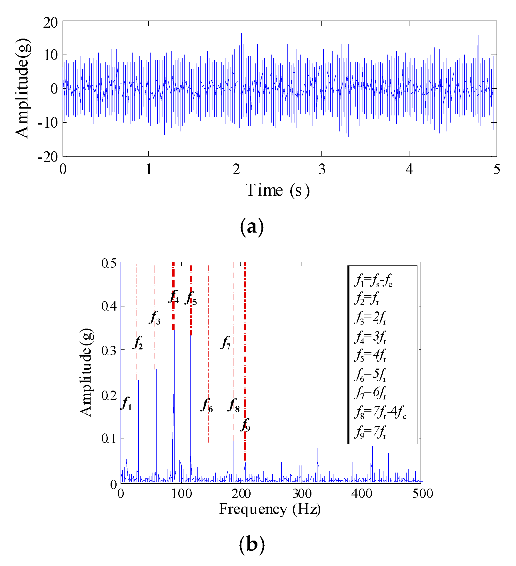

Figure 20.
Improved wavelet scalogram analysis. (a) Reassigned scalogram; (b) Scalogram under synchronous averaged.
Figure 20.
Improved wavelet scalogram analysis. (a) Reassigned scalogram; (b) Scalogram under synchronous averaged.
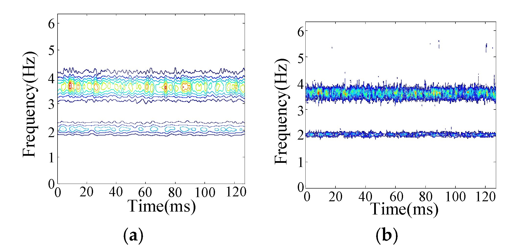
Figure 21.
Wavelet ridge of bearing signals for improved wavelet scalogram.

Figure 22.
Time domain waveforms and spectrum of instantaneous amplitude. (a) Waveform of instantaneous amplitude; (b) Spectrum for instantaneous amplitude.
Figure 22.
Time domain waveforms and spectrum of instantaneous amplitude. (a) Waveform of instantaneous amplitude; (b) Spectrum for instantaneous amplitude.

Table 1.
Parameters for planetary gearbox and planetary bearing.
| Configuration Parameter | Parameter Values |
|---|---|
| The number of sun gear tooth | 17 |
| The number of planet gear tooth | 35 |
| The number of annular gear tooth | 88 |
| The number of planet gear | 3 |
| Transmission ratio | 6.176 |
| Type of planetary bearing | 204 NJ |
| The number of planetary bearing roller | 11 |
| The bearing pitch diameter | 34 mm |
| The planetary rolling element diameter | 7.493 mm |
| The planetary bearing contact angle | 0° |
Table 2.
Parameters for failure experiment system.
| Characteristic Frequency | Frequency Values |
|---|---|
| Sampling Frequency | 12,800 Hz |
| The rotation speed | 1800 rpm |
| The rotation frequency of sun gear | 30 Hz |
| The rotation frequency of planet carrier | 4.86 Hz |
| The relative rotation frequency of planet gear | 12.21 Hz |
| The absolute rotation frequency of planet gear | 7.36 Hz |
| Bearing outer ring fault characteristic frequency | 31.53 Hz |
| Bearing inner ring fault characteristic frequency | 49.38 Hz |
© 2018 by the authors. Licensee MDPI, Basel, Switzerland. This article is an open access article distributed under the terms and conditions of the Creative Commons Attribution (CC BY) license (http://creativecommons.org/licenses/by/4.0/).
Share and Cite
MDPI and ACS Style
Li, H.; Yang, R.; Wang, C.; He, C. Investigation on Planetary Bearing Weak Fault Diagnosis Based on a Fault Model and Improved Wavelet Ridge. Energies 2018, 11, 1286. https://doi.org/10.3390/en11051286
AMA Style
Li H, Yang R, Wang C, He C. Investigation on Planetary Bearing Weak Fault Diagnosis Based on a Fault Model and Improved Wavelet Ridge. Energies. 2018; 11(5):1286. https://doi.org/10.3390/en11051286
Chicago/Turabian StyleLi, Hongkun, Rui Yang, Chaoge Wang, and Changbo He. 2018. "Investigation on Planetary Bearing Weak Fault Diagnosis Based on a Fault Model and Improved Wavelet Ridge" Energies 11, no. 5: 1286. https://doi.org/10.3390/en11051286
Note that from the first issue of 2016, this journal uses article numbers instead of page numbers. See further details here.