1. Introduction
Transportation is the principal source of energy consumption, pollutants, and carbon emissions. Energy consumption and pollutant emissions vary greatly for different transport modes [
1]. Since high speed rail (HSR) has the potential to provide passengers with another more environmentally friendly and convenient transport option, many countries have developed or are developing such systems. According to statistics from UIC (International Union of Railways) [
2], the total HSR lines operating worldwide are now 41,222 km. In addition, about 14,511 km of new HSR lines are now under construction, and more than 8268 km of HSR lines are being planned, and such rail systems are increasingly important in regional passenger transport markets. From the viewpoint of energy consumption, the California High-Speed Rail Authority and Federal Railroad Administration [
3] estimated that an electrically powered HSR will use only one-third of the energy of airplanes and one-fifth of the energy of private cars per passenger, reducing dependence on foreign oil by 12.7 million barrels and greenhouse gas emissions by 12 billion pounds per year. In addition, HSR also offers passengers shorter travel times with the operating speed reaching 350 km/h on the Beijing–Tianjin and Wuhan–Guangzhou routes in China, as well as greater capacity, with the double-decked E4 Series Shinkansen able to carry 1634 seated passengers, double the amount of an Airbus A380. These positive features mean that HSR is becoming a popular alternative passenger transport mode, and such systems are now widely regarded as one of the most significant technological breakthroughs in the public transportation industry of the late 20th century [
4].
HSR has significantly impacted the market shares of other transportation modes in countries like South Korea, Japan, France, Spain, Germany, and Taiwan [
5]. For instance, the first stage of the HSR in Korea, the Korean Train Express (KTX), started operation between Seoul and Busan (about 410 km) on April 2004 with a speed of 300 km/h. KTX reduced rail travel time between Seoul–Busan from 4 h 27 min to 2 h 40 min. It carried over 10 million passengers in the first five months of operating. In a survey carried out in April 2004, the results showed that KTX had attracted 56% of its passengers from the existing conventional rail service, 17% from air, and 15% from express buses [
6]. In Japan, the Tokaido Shinkansen is the world’s busiest HSR line and links the country’s three largest metropolitan areas, Tokyo, Nagoya, and Osaka. The operating speed has increased from the initial 210 km/h to 285 km/h, and 6 billion people had used the Shinkansen. The Nozomi train takes about 2 h 22 min to travel between Tokyo and Osaka, which is almost the same time using airline transportation service, when including travel between the airports and city centers, check-in, and transit. Therefore, although airline companies offer discounts between Tokyo and Osaka, the Shinkansen still maintains an 86% market share on this route. In addition, from the view of environmental feasibility, the energy consumption amount per seat of HSR when traveling between Tokyo and Osaka is approximately 1/8th of that of an aircraft, and the CO
2 emission rate for the same is around 1/12th [
7]. In the case of France, the Train à Grande Vitesse (TGV) entered into service in 1981. The total operating route length was 1896 km in January 2011, with a maximum service speed of 270–320 km/h. Park and Ha [
8] noted that once the eastern HSR route was completed, the Paris–Lyon route (450 km) of the HSR decreased the air transport volume share from 30% to 15%, the Paris–Marseilles route (700 km) dropped from 45–55% to 35–45% and the Paris–Nice route (900 km) reduced from 55–65% to 50–60%. In Spain, the HSR network, Linea de Alta Velocidad (L.A.V.), has been operating since 1992. There are four main lines, as follows: L.A.V. Madrid–Sevilla, L.A.V. Madrid–Valladolid, L.A.V. Córdoba–Málaga, and L.A.V. Madrid–Barcelona, with an operating speed of 270–300 km/h. The total length of the system was 2056 km in January 2011, and there are 1767 km of L.A.V. lines under construction. De Rus and Inglada [
9] found that the HSR decreased the market share of domestic air carriers from 25.1% to 2.8%, buses from 8.7% to 5.3%, and conventional train from 14.2% to 2.8% along the Madrid–Seville route (471 km). Similarly, Coto-Millán et al. [
10] argued that the new HSR line running from Madrid to Barcelona route (621 km) will reduce the market share of air carriers from 69.4% to 38.2%, buses from 4.6% to 3.7%, and conventional trains from 6.1% to 1.4%. On the Madrid–Seville route, an airplane takes 50 min, a bus takes 6 h 30 min, conventional rail takes 5 h 35 min, and the HSR takes 2 h 25 min. On the Madrid–Barcelona route, a plane takes 55 min, a bus takes 7 h 35 min, conventional rail takes 6 h 35 min, and the HSR takes 2 h 35 min. The studies of the various HSR systems currently in operation outlined above demonstrate that they all had a significant impact on the market share of existing transportation modes.
The statistical data also indicates that the introduction of an HSR system will affect the regional transport market. For example, Vickerman [
11] examined the French TGV and analyzed the fluctuations in rail, air, and TGV passengers on the routes served by the system, and concluded that the HSR has a clear advantage in offering faster travel time on the order of one to three hours for distances of 200–600 km. At shorter distances, the study found that it was difficult for the HSR to compete with cars, while at longer distances air transport was more competitive. Givoni [
12] observed the operation of HSR systems on the routes of London–Paris, Tokyo–Nagoya and Brussels–Paris, and found that the competition of HSR would vary with the trip distance. For instance, the observations of Tokyo–Nagoya and Brussels–Paris showed that the HSR service is regarded as a good substitute for air transport on routes of around 300 km. However, the substitution effect disappears for routes of around 1000 km and above, such as the Tokyo–Fukuoka route. In between these distances, there is usually a direct competition between the HSR and air transport. In the review of the related literature, Givoni and Banister [
13] analyzed the competition between HSR and air transport, and concluded that HSR substituted the aircraft on the routes of up to 800 km by offering comparable and even shorter travel times between city centers. Fröidh [
14] defined the competitive relationship between HSR and air transport by travel time segments for the Swedish domestic market. Similarly, Ureña et al. [
15] gathered research data related to the travel share between different transport modes for various travel distances. They concluded that intercity HSR services are in competition with air transport when there is a travel time of less than three hours, and that 65% of passengers prefer to use the HSR when their travel time is under two and a half hours.
The works reviewed above demonstrate that the competitiveness of an HSR system depends on the travel distance or travel time. However, the findings of these past studies on the impact of HSR on regional transport markets are generally not based on appropriate quantitative approaches. Therefore, how to develop a systematic model to uncover the competitive characteristics of regional transport modes, such as their long-run relationships and short-run dynamics, remains an important task. In reality, competitive relationships are neither monotonic nor static. A short-run dynamic would be accompanied by a long-run relationship, and thus the dynamics in the short-run have to be considered. To construct the systematic model, time series analysis provides an econometric methodology for modeling the dynamic competition between two or more variables. We can check the existence of a long term (equilibrium) relationship through the co-integration test, while the Granger causality test can be used to confirm their causal relationship. The short-run dynamic relationship can be estimated by the Vector Error Correction (VEC) model. In addition to understanding the short-run dynamic relationships between variables, we can further examine how those variables adjust with each other in order to comprehend their long-run relationship. Using the impulse response and variance decomposition tests, we can trace the response of one variable to a change in another one in a dynamic system, and estimate the percentage of the forecast error variance of each of the variables that can be explained by exogenous shocks to the other variable. In this study, we apply time series analysis to model the dynamic competition in a regional passenger transport market when an HSR is introduced. This study does not consider a regional transport market with distances that are either too short or too long for an HSR to be competitive with other modes. The model developed in this work used to analyze comprises the long-run and short-run dynamic relationships. The vector autoregressive (VAR) model is applied as our basic model for the subsequent co-integration test, Granger causality test, VEC estimate, impulse response test, and variance decomposition test. The VAR model was employed by Bjørner [
16] to analyze the long-term effects of taxes on freight transport and traffic volume. Kulshreshtha et al. [
17] applied the same approach to evaluate the long-run structural co-integrating relationship, short-run dynamics, and the effects of shocks on economic growth and freight transport demand in Indian railways. In addition, Coto-Millán et al. [
18] investigated the long- and short-run relationships both for Spanish maritime exports and imports using the VAR model. Similarly, Yap et al. [
19] employed a similar method to analyze the long- and short-run competitive dynamics between the major container ports in East Asia. In addition, Marazzo et al. [
20] studied the relationship between air transport demand and economic growth in Brazil using a co-integration test, VEC estimate, Granger causality test, and impulse response analysis. It can thus be seen that the VAR model and the related analytical methods have been widely employed in the transportation field.
The rest of this paper is organized as follows.
Section 2 explains the processes of model construction used in this study.
Section 3 briefly describes the background of the case study and the sources used in the data collection. The empirical findings about dynamic competition are presented in
Section 4, while
Section 5 summarizes our conclusions.
2. Model Construction
As the main objective of this study is modelling the dynamic competition due to the introduction of an HSR in the market for regional passenger transport, a unit root test, co-integration test, Granger causality test, VECM (Vector Error Correction Model), impulse response test, and the variance decomposition test were applied to analyze the passenger volume data. To conduct these tests, we constructed a VAR model as the basis, and the following paragraphs describe the detailed modelling procedures.
Although the prior assumption of VAR is that the vector stochastic process is stationary, implying that the time series data is time-invariant, time series data such as monthly passenger volume in each transport mode are often non-stationary. This causes the regressions to generate significant coefficients, regardless of there being no real relationships among the variables, and this leads to the problem of spurious regression. It is thus necessary to confirm whether the raw data have to be transformed into stationary data, and so a unit root test first needs to be conducted in order to check the stationary properties of the data sets. The null hypothesis of non-stationary process is tested against the alternative of a stationary process through the Augmented Dickey–Fuller (ADF) technique [
21]. In addition, this procedure is carried out before the co-integration test, because only the variables which have the same order can be co-integrated. The order of integration for each variable can be ascertained through the ADF test. If the levels of variables exhibit a non-stationary process, the differences have to be applied
d times to make the process stationary. The non-stationary process is represented by I(
d) which
d ≥ 1. On the other hand, the levels of the variables are stationary when
d = 0. The ADF test is based on the following equation:
where
yt,j is the passenger volume of transport mode
j at time
t,
, C is a constant term, Θ is the trend term with coefficient
βj,
pj is the number of lags necessary to obtain white noise for transport mode
j,
εt,j is the error term, and
φj and
ψi,j are the coefficients.
The Akaike information criterion (AIC) [
22] is utilized to determine the appropriate lag length
pj. The null hypothesis H
0 of ADF test is that
yt is I(1) against the alternative H
1 that
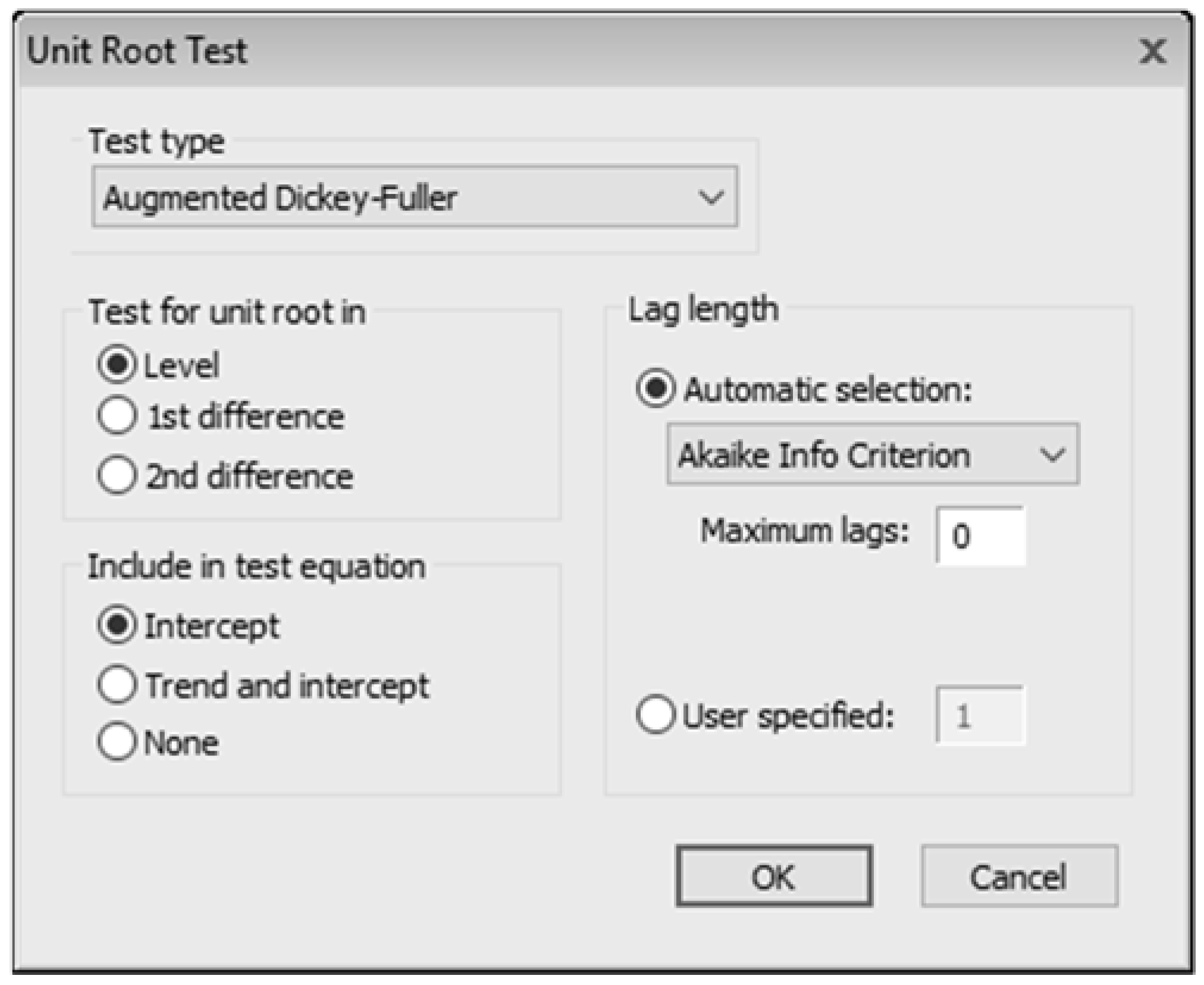
yt is stationary which is shown as I(0). If the ADF test does not reject the null hypothesis, it is necessary to test for higher orders of integration until the null hypothesis is rejected. The ADF test can be performed in EViews and is shown as
Figure 1.
Taking one of our empirical study data (HSR) as an example, the results are described as
Table 1 and
Table 2.
Table 1 presents information about the ADF statistic result, associated critical values, and the
p-value. The ADF statistic value is −2.141178 which is greater than the critical values so that we do not reject the null hypothesis that HSR has unit root.
Table 2 shows the intermediate test equation that we used to calculate the ADF statistic.
For those time series variables having the same integration order, the co-integration test is used to check whether there are any long-run relationships between the transport modes. By applying Johansen’s methodology for modelling co-integration [
23], transport modes with the same I(
d) are analyzed pairwise to test their co-integration relationships with the passenger volume. The procedures of the Johansen’s approach applied in this study are described as follows.
Let
Yt = (
yj,t,
yj’,t)’ denote a 2 × 1 vector with the passenger volumes of transport mode
j (
yj,t) and transport mode
j’ (
yj’,t) at time
t. Series
yj,t and
yj’,t are stationary with the same I(
d). Consider the basic form of the VAR(
p) model with
p-lag:
where
Πi is a 2 × 2 coefficient matrix,
p is the lag length that determined by the sequential modified likelihood ratio (LR) test statistic, and
εt is a 2 × 1 zero mean white noise residual vector. The residuals of the VAR model are examined by the Q-test and Jarque-Bera test to ensure that they are not auto-correlated and are normally distributed.
Suppose that there are
r co-integrating relationships in
Yt. There then exists a 2 ×
r vector
β such that
β’Yt is I(0). To ensure the uniqueness of this linear combination, we normalize
β and
βn such that
μt ∊
μt is I(0). The linear combination of
is called the co-integrating equation (CE), which can be used to infer the stochastic long-run relation of passenger volume between transport mode
j and mode
j’.
In order to estimate the matrix of co-integrating vectors
β, we have to find out the rank of
Π first, because
Π and
β have the same rank. The sequential procedures of Johansen’s trace statistic test can be used to determine the number of co-integrating vectors. Suppose that
and
are the estimated eigenvalues of
Π and that the sample size of time series is
T. Johansen’s approach is to test whether
r =
r0 against
r >
r0, where
r0 = 0, 1 and the trace statistic is defined by
Accordingly, the first step is testing whether r = 0 against r > r0. If the null hypothesis is rejected, it implies that there is at least one co-integrating vector. A similar test process can continue to test H0 (r = 1) against H1 (r > r0). Because Π has only two eigenvalues, this test stops at r0 = 1, and hence there is at most one co-integrating vector between yj,t and yj’,t.
Once the long-run relationship between transport modes has been proved, we can use the same VAR(
p) model to examine their long-run causal relationships. The Granger causality relationship is detected through the Wald
χ2(
p) test [
24,
25]. The null hypothesis of the Wald test statistic is non-Granger causality from transport mode
j to mode
j’ and vice versa. If both events exist simultaneously, it is said that feedback exists between transport mode
j and mode
j’.
In order to capture both short-run dynamics and the long-run relationship between transport modes, we transform the VAR model in Equation (2) to the VECM [
26].
where
Π equals
, and
for
i = 1,…,
p − 1.
The vector Γi in Equation (5) is called the short-run impact matrix, and its value can be estimated by the maximum likelihood approach. We can obtain the short-term dynamics between transport modes from the findings of Γi. Similarly, we apply the Granger causality test on VECM to understand the causal relationships between short-run coefficients.
Finally, the impulse response test and the variance decomposition test are employed to track the impact of HSR on the existing transport modes, and obtain an estimate of the percentage of the forecast error variance of each of the transport modes that can be explained by exogenous shocks to the other one. The impulse response function was proposed by Hamilton [
27] and the matrix form is as follows.
where
,
εt−i denotes the error term at time
t −
i does not included at time
t −
i + 1, C denotes the vector of constant,
ψ denotes the matrices of coefficients to be estimated.
From Equation (6), the effect of a one-time shock to one of the innovations on current and future values of the endogenous variables can be presented by differentiating the function with respect to
εt−i as
where
ψi is response
Yt to
Yt innovations.
The variance decomposition is applied to measure the amount of influence variables have in the model which produces the cumulative effect of one transport mode on another one over time. The relative importance of the transport modes can be obtained through the analysis. The variance decomposition is shown as
where
is the variance degree of
yt forecast
n-periods ahead caused by
,
is the variance degree of
xt forecast
n-periods ahead caused by
.
3. Empirical Study and Data Collection
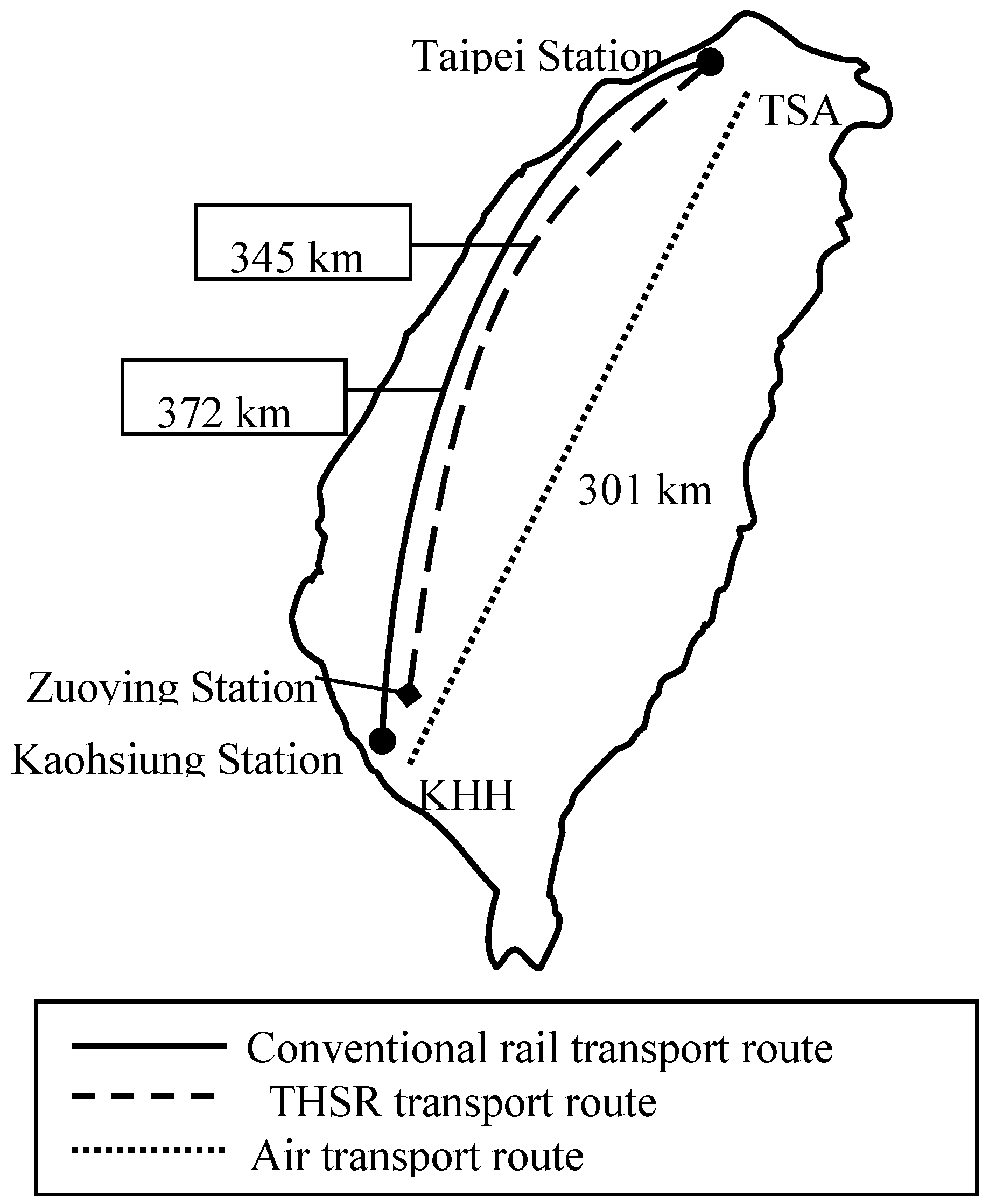
This section illustrates how to model dynamic competition for a regional transport market using our approach and a time series analysis. We use the passenger transport market of Taiwan as our empirical study case. Taiwan is an island located off the southeastern coast of China in East Asia in the Western Pacific Ocean. The main island is 394 km long and 144 km wide and the total land area is about 36,191 square kilometers. The eastern side of Taiwan consists mostly of rugged mountains from the northern to the southern tip of the island. Therefore, most of Taiwan’s population and economic activities are located on the flat western side. Taipei is the most densely populated city, and is located in northwestern Taiwan, followed by Kaohsiung in the southwest. Before the introduction of the HSR, travelers journeyed along the western corridor by air, conventional railways, long distance bus carriers, and private cars. There were four airlines, Mandarin Airlines, TransAsia Airways, Far Eastern Air Transport and UNI Air, serving the Taipei–Kaohsiung route, and the number of flights exceeded 100 per day during peak years, when it was the most profitable domestic route. The travel time is 55–60 min between Taipei Sungshan Airport (TSA) and Kaohsiung Hsiaokang International Airport (KHH), with a distance of 301 km. Before the HSR was launched, air was the fastest transport mode between Taipei and Kaohsiung. The Taiwan Railways Administration (TRA), which operates the conventional railway system, is an agency of the Ministry of Transportation and Communications (MOTC), and the western line connecting Taipei and Kaohsiung is the busiest in Taiwan. Conventional trains take 274–517 min to run between Taipei Station and Kaohsiung Station, with a route length of 372 km.
As Taiwan’s economy has had dramatic growth over the past few decades, there has also been a rapid increase in the demand for transportation services. As the original transport systems began to be saturated, the MOTC began considering developing an HSR system to serve the western corridor [
5]. The government decided to build the HSR system using a Build–Operate–Transfer (BOT) model, and US
$18 billion was invested in the project. The MOTC signed the Taiwan High Speed Rail Construction and Operation Contract and Station Area Development Contract with Taiwan High Speed Rail Corporation (THSRC) in July 1998, and the THSRC began running its train service in January 2007. The total operating length of the HSR along the west coast of Taiwan is about 345 km, and the service requires only 96–120 min between Taipei Station and Kaohsiung Zuoying Station, with an operating speed of about 300 km/h.
Figure 2 shows the present status of transport routes between Taipei and Kaohsiung for the conventional rail, THSR, and air transport modes.
The introduction of the THSR had a considerable impact on the original transport market, and transport operators struggled to maintain their market share in the corridor and adopted various promotional strategies to achieve this. However, it is difficult to conduct a systematic analysis of the regional transport market to uncover the impact of the THSR simply by examining changes in the market share of different modes [
5,
28]. Therefore, it is necessary to apply our model to better understand the dynamic rivalry between THSR and the conventional rail and air transport in Taiwan from a regional market point of view [
29,
30,
31,
32,
33,
34]. From the analysis based on the model, we can reveal the trend of influence between transport modes, and these findings can be utilized as forecasting references [
35,
36,
37,
38,
39]. To construct our model, the monthly passenger volume for those who travel between Taipei and Kaohsiung was extracted to model the dynamic competitive relationships in Taiwan’s public transportation market [
40,
41,
42]. The passenger volumes of air transport, conventional rail transport, and HSR transport were collected from the MOTC and THSRC. Because the THSRC started its HSR commercial service in January 2007, the data is collected from January 2007 to May 2010, and thus there are 41 monthly observations of passenger volumes for the air, conventional rail, and THSR transport respectively. The results of the empirical study are given in the next section.
4. Empirical Findings of Dynamic Competition
To model the HSR’s effects on dynamic competition in the regional passenger transport, the THSR passenger volume is set as the independent variable (IV), and the conventional rail passenger volume and air passenger transport volume are set as dependent variables (DV) in the long-run analysis. In the following report on the results, the THSR passenger volume is written as HSR, the air passenger transport volume is represented as AIR, and the conventional rail passenger volume is denoted as RAIL. The first step is to examine the stationary properties and order of integration for the time series data by using a unit root test, as in Equation (1).
Table 3 shows the results of the ADF stationarity test. All transport modes exhibited stationarity as the null hypotheses, and the ADF statistics were rejected at a 5% significance level for all time series data. We thus conclude that all the variables considered in this study are I(0) series. The time series of transport modes’ passenger volume with the same integration order were paired to analyze their dynamic relationships. Accordingly, the pairs of HSR-AIR and HSR-RAIL were used to construct the VAR models.
The sequential modified LR test statistic is applied to determine the appropriate lag length of the VAR(
p) model for each paired transport mode. According to Equation (2), the basic VAR models for HSR-AIR and HSR-RAIL are constructed as VAR(8) and VAR(3), respectively. The white noise residuals of both of these modes are ensured by the Q-test and Jarque-Bera test.
Table 4 shows the results of Johansen’s co-integration test, in which we can determine whether a pair of time series data is co-integrated or not. The trace statistic is estimated by Equation (4). The pairs of HSR-AIR and HSR-RAIL have long-run equilibrium relationships because their trace statistics reject the null hypothesis of no CE at the 5% critical value. Therefore, there exists at least one CE for each paired transport mode. In other words, the long-run relationships existing between THSR and conventional rail and that between THSR and air transport are proved.
The estimated CEs from the Equation (3) and Granger causality test results are summarized in
Table 5. As the coefficients of CEs for the pairs of HSR-AIR and HSR-RAIL are −0.2485 and −0.0665, respectively, there is a negative long-run equilibrium relationship within these paired transport modes on their series of passenger volumes. In addition, the pair of HSR-AIR shows a significant negative time trend. This means that besides the influence of HSR, the passenger volume of air is declining over time. To confirm the causal relationship between the transport modes, a Granger causality test is conducted. The null hypotheses of the Wald test statistic for the pairs of HSR-AIR and HSR-RAIL are rejected at the 1% significance level. The Granger causality relationships from HSR to AIR and from HSR to RAIL are proved. To sum up, the operation of THSR generated a negative long-term effect on conventional rail and air transport. Meanwhile, the negative effect on conventional rail is weaker than that on air transport.
After the pairs of HSR-AIR and HSR-RAIL were found to have long-run equilibrium relationships in VAR(
p) models, their short-run causal relationships and dynamic statuses were analyzed under the VECM, as in Equation (5). The estimates of short-run dynamic coefficients and Granger causality test results for pairs of HSR-AIR and HSR-RAIL are summarized in
Table 6.
We first check the causal relationships of the HSR-AIR pair. The Wald test statistic for the null hypothesis of no Granger causality from the first difference of HSR to the first difference of AIR is 7.4411, which cannot be rejected at the 10% significance level. The null hypothesis of no Granger causality from ∆(AIR) to ∆(HSR) is rejected at the 1% confidence level. This thus implies that short-run causality exists from ∆(AIR) to ∆(HSR) but not from ∆(HSR) to ∆(AIR), as the coefficients on ∆(HSR-1) to ∆(HSR-8) of ∆(AIR) are insignificant. The negative short-run dynamics from AIR to HSR are found because the coefficients on ∆(AIR-1) to ∆(AIR-6) of ∆(HSR) are negative and significant at the 1% level. In addition, the previous period of HSR also exhibited a significant negative impact on itself. Nevertheless, the coefficients show that the impact of air transport is much stronger than the THSR itself, which implies that an increase in air passenger transport volume can be used to predict a decrease in THSR passenger volume in the short term, and vice versa. For the pair of HSR-RAIL, no short-run causality is found from ∆(RAIL) to ∆(HSR) since the Wald test statistic of 2.2907 is insignificant. On the other hand, ∆(HSR) has a short-run causal relationship with ∆(RAIL) at the 10% confidence level. The previous periods of HSR and RAIL itself have a positive impact on the first difference of RAIL. In addition, the coefficients indicated that the positive impact of conventional rail itself is stronger than that of the THSR.
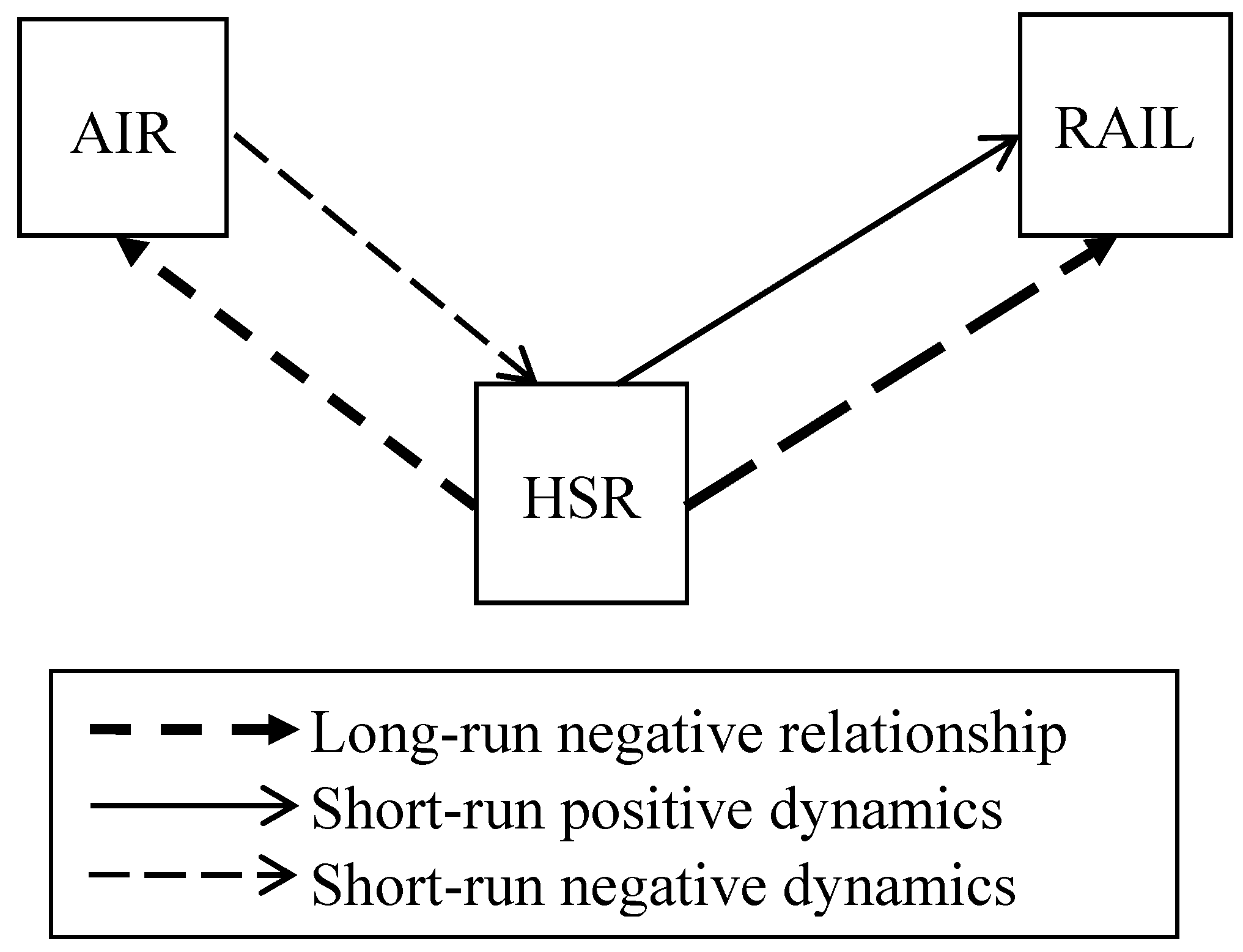
To summarize the results, in
Figure 3 we present the long- and short-run impacts, and the Granger causality relationships between these three transport modes. All of the relationships among the transport modes show unidirectional Granger causality. In general, the relationship between THSR and air transport is mutually competitive. The introduction of the THSR had a negative impact on air transport in the long-run, while in the short term the handling performance of air transport appeared to have a negative impact on THSR. Conventional rail was negatively affected by THSR in the long-run, as was air transport. However, in the short-run, the dynamics of the THSR exhibited a positive influence on conventional rail. In other words, there is a complementary relationship between THSR and conventional rail in the short term.
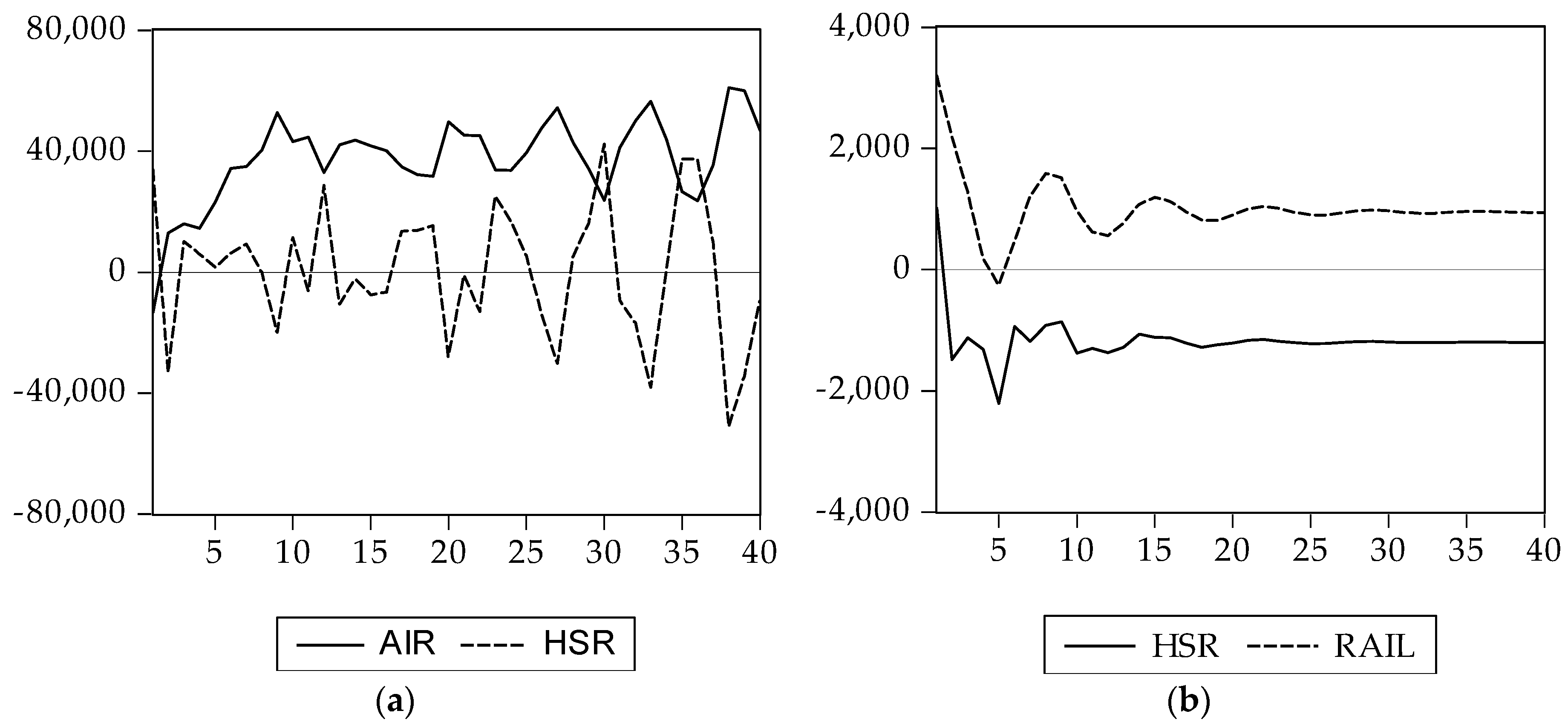
To conduct a further analysis, we also examined the impact of shocks to one transport mode on the other modes in the VAR model using the impulse response function, as shown in Equation (6). The impulse responses of the paired HSR-AIR and HSR-RAIL are shown in
Figure 4, which presents the dynamic effects of one standard deviation (S.D.).
For (a) HSR-AIR, AIR is mainly affected by itself in the first year and the response of AIR to the shocks of HSR is relatively flat. On the other hand, the response of HSR to the shocks of AIR is positive. The air passenger volume can be seen as a sign of the passenger transport market. The impacts on HSR from itself are dynamic and have the opposite effect to the shocks of AIR, which shows their mutually competitive status. The impulse responses of the paired HSR-RAIL are shown on the right side of
Figure 4. In the first five months, the RAIL responds negatively to the shocks of HSR and itself, and then the negative impacts on RAIL from HSR are greater than the positive impacts from itself. In contrast, the response of HSR to the shocks of itself is positive and greater than the negative response to the shocks of RAIL.
After the main source of shocks between transport modes has been found, the variance decomposition is applied, as in Equation (7), to interpret the contribution of these shocks by computing the percentage of the variance of the
n-period ahead of forecast error.
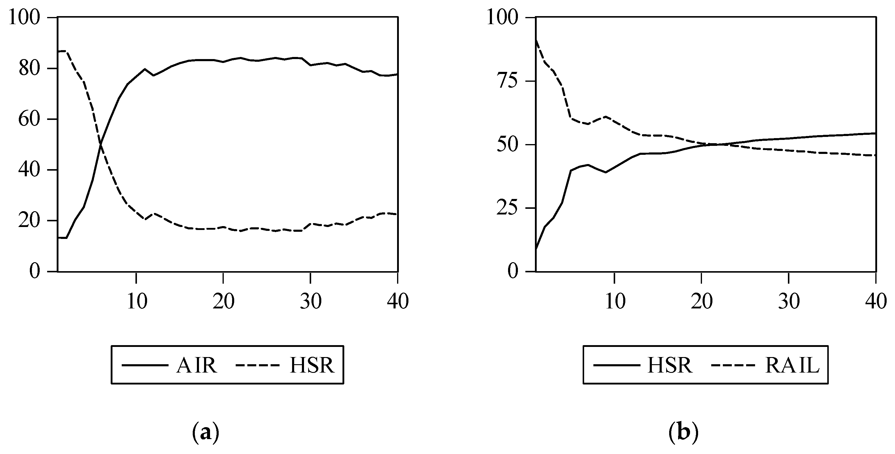
Figure 5 presents the variance decomposition results for the pairs of HSR-AIR and HSR-RAIL. The left part of
Figure 5 shows that the variance of AIR is mainly explained by itself. This phenomenon implies that airlines decreased the flights to deal with the introduction of the THSR. The flights on the Taipei–Kaohsiung route declined from 1948 flights per month to 1377 flights per month in the first year of THSR’s operation. After the THSR had been running for 14 months, two airlines withdrew from the market, leaving two airlines continuing to provide their services. The policies adopted by the airlines caused greater changes in the passenger volume than the impact of the THSR. The 87% variance of HSR can be explained by itself in the first month. However, the impact of AIR increases after 14 months, and the shock of AIR can explain up to 80% of the variability in HSR. The variance decomposition results for the pair of HSR-RAIL are presented on the right side of
Figure 5. In the first nine months of the THSR’s operations, the variance of RAIL is mainly interpreted by itself. In the long-run, the percentages of explanation for the variance of RAIL are about 70% by HSR and 30% by RAIL itself. With regard to the variation of HSR, HSR explains approximately 80% of the forecast error variance for itself and the influence of RAIL is only 20%.
5. Conclusions
This study provides an econometric model to analyze the dynamic competition for regional passenger transport. The model cannot only be used to better understand the relationships among transport modes, but also presents comprehensive information regarding their long- and short-run influences. This information cannot be obtained from a simple statistical analysis, but is extremely useful for transport carriers, regional governments, and transportation authorities. The model provides another practical and detailed analytic dimension for operational or forecasting references. Transportation operators can use it to identify their market orientation, and adopt active strategies and tactics that are appropriate for their dynamic market status. At the regional government level, related administrators can utilize the analysis to undertake better city planning and development. In addition, transportation authorities can refer to the information presented by the model when making their infrastructure investment decisions, which develops better public transportation plans. A good public transport plan not only considers transport carriers, but also facilitates social development and general welfare. As Maciel et al. [
43] mentioned that the more a transportation system relies on public transportation, the more sustainable the system becomes. On the other hand, an unsustainable transportation system leads to public diseconomy in a waste of social, financial, natural, and energy resources.
While the introduction of an HSR system provides passengers with an environmentally friendly, convenient, and timesaving alternative, it also disrupts the existing passenger transport market. This study adopts time series analysis to model the dynamic effects of the introduction of an HSR system in a regional passenger transport. The analyses include examining the long-run equilibrium and causal relationships, and the short-run causality and dynamic relationships between transport modes. In addition, based on the model we can conduct impulse response tests and variance decomposition tests to further understand the interactions between two transport modes. The case of Taiwan’s regional passenger transport was adopted in our empirical study, and the findings indicate that the THSR has had a negative impact on conventional rail and air transport in the long-run. In addition, the results show that a competitive relationship exists between THSR and air transport in both the short and long term. In the short-run dynamics, the air passenger transport volume could be regarded as a good predictor of THSR passenger volume. In turn, the THSR passenger volume could be used to predict conventional rail transport volume. Different from the long-term relationship, the operations of THSR and conventional rail are complementary in the short term. From the short-run market viewpoint, the THSR and conventional rail meet different kinds of passenger demand. Therefore, a previous increased passenger volume for the THSR implies an overall increasing demand for regional transport. Consequently, the past increased THSR passenger volume could be used to predict the growth of conventional rail transport. The analysis results lead to the following conclusions: the introduction of an HSR system would share the existing market with air transport and conventional rail transport in the long-run market equilibrium status. These findings correspond with those of previous research, which found that HSR has clear advantages with travel times of one to three hours and distances of 200–600 km. The proposed model is flexible and robust for practical applications. Therefore, we can also observe the short-run dynamic relationships of the three transport modes. Through the impulse response test, we can further track the responses of the three transport modes to the shocks from themselves and each other. The variance decomposition test is used to examine the degree of explanation for the variance of transport modes. However, the short-run dynamic relationships may vary with different strategies taken by transport carriers or other influence factors. As for our empirical study case, the airlines took the strategy of withdrawal from the market. All airlines provided their services on the Taipei-Kaohsiung route until September of 2012. Passengers have lost the option of air transport since then. If airlines had adopted different policies to deal with the competition, we may have got another result in the short-run observation.
Future research might collect the time series data for a longer period and update the data at any time to continue to observe the changes in the transportation market. In addition, there are other time series models, such as the autoregressive distributed lag model (ARDL), autoregressive integration moving average model (ARIMA), vector autoregressive moving average model (VARMA), and Bayesian model, that can be applied to predict the traffic volume for different transport modes, and their forecasting performance can then be compared based on the empirical evidence to find out the optimal forecasting model for each mode. Further, our model can also be applied to other similar regional transport markets in future research.

 ,
, 


