Probabilistic Electricity Price Forecasting Models by Aggregation of Competitive Predictors

Abstract

This article presents original probabilistic price forecasting meta-models (PPFMCP models), by aggregation of competitive predictors, for day-ahead hourly probabilistic price forecasting. The best twenty predictors of the EEM2016 EPF competition are used to create ensembles of hourly spot price forecasts. For each hour, the parameter values of the probability density function (PDF) of a Beta distribution for the output variable (hourly price) can be directly obtained from the expected and variance values associated to the ensemble for such hour, using three aggregation strategies of predictor forecasts corresponding to three PPFMCP models. A Reliability Indicator (RI) and a Loss function Indicator (LI) are also introduced to give a measure of uncertainty of probabilistic price forecasts. The three PPFMCP models were satisfactorily applied to the real-world case study of the Iberian Electricity Market (MIBEL). Results from PPFMCP models showed that PPFMCP model 2, which uses aggregation by weight values according to daily ranks of predictors, was the best probabilistic meta-model from a point of view of mean absolute errors, as well as of RI and LI. PPFMCP model 1, which uses the averaging of predictor forecasts, was the second best meta-model. PPFMCP models allow evaluations of risk decisions based on the price to be made.

1. Introduction

The dynamic nature of most of the natural or artificial systems and the human necessity to ensure their correct performance in the future have led to the development of forecasting techniques. A decision maker needs forecasts of his/her variables of interest if there is uncertainty about their future values. Forecasting involves the use of available information to predict the likely value of these variables. In the electric power sector, the implantation of liberalized electricity markets has changed the behaviour of producers and costumers. In the past, before the new regulation, power producers had the minimal financial risks, as customers were not able to acquire freely electricity. Now, with a competitive market agents can sell or buy energy like any other commodity.

On the other hand, the growing penetration of renewable energy generation into the power systems has increased the uncertainties about the short-term generation values. These uncertainties are caused by the intermittent nature of wind, solar or hydro based generation, and their associated risks are also influenced by the own uncertainties in the demand of customers. In a competitive electricity market, agents’ bidding strategies are very dependent of the expected electricity prices.

Electricity markets show very volatile and dynamic behaviours as they depend on a large number of variables, such as electricity demands, prices of the raw materials used in thermal generation, the intermittence and seasonality of renewable sources of electricity production (wind power, photovoltaic and hydro generation), etc. The anticipated knowledge of the prices that will be fixed for the following days in the day-ahead market can determine the trading strategies of the agents involved in the electricity markets, allowing them to select the product or even the market that best suits their interests.

The agents involved in a day-ahead electricity market are users of diverse type of forecasting services. There are companies specialized in price forecasting that sell forecasts to agents. These forecast provider companies (with their own predictors, that is, price forecasting tools) can be classified as: (a) professionals, who have restricted and confidential information although they use simpler techniques than other forecasting sellers; (b) academics, who utilize more basic information but very complex and technologically advanced techniques. Each predictor uses different information and applies the most varied models and methods of data processing to obtain its forecasts. A provider company does not usually communicate the forecasting methodology of its own predictor to its competitors.

In the international literature, tens of articles describing electricity spot price forecasting (SPF) models have been published in the last two decades [1,2]. These models provide forecasts of prices without any other information. SPF models have been developed using a variety of techniques such as time series based models [3,4,5,6,7,8], linear regression [4,9,10], Generalized Auto-Regressive Conditional Heteroskedasticity (GARCH)-type models [8,11], artificial neural networks [4,5,6,12,13,14,15], support vector machines [16,17,18] and fuzzy systems [19,20,21]. Many models use a hybrid approach combining two or more techniques or complex optimization and/or pre-processing methods [18,22,23,24,25,26,27,28]. The main limitation of SPF models focuses on their insufficient forecast information for trading purposes since they do not offer the uncertainty associated with the forecasts.

Probabilistic models aim to overcome the main limitation of spot forecasts, allowing the assessment of the uncertainty associated with the forecasted values. In recent years, the increasing penetration of electric energy based on renewable sources and the new smart grids have increased the uncertainty of the future demand, generation and electricity price [29,30]. Three classes of probabilistic electricity price forecasting (PEPF) models have been reported in the literature [1]: interval forecasts or prediction intervals (PIs), density forecasts, and threshold forecasting. The PEPF models that provide PIs are the most common. PIs can help market agents to submit bids with low risk [31]. Several methods have been applied to obtain PIs forecast models from the point predictions of SPF models [30]:

• Historical simulation, which uses sample quantiles from the empirical distribution of one step ahead prediction error (difference between the real value and that provided by SPF models). Different kinds of SPF models have been used in historical simulation, from autoregressive models [7,32] to semiparametric models [32].
• Distribution-based probabilistic forecasts, which basically assume a probability density function (PDF) for the prediction errors; the standard deviation of the error density is calculated and the lower and upper bounds of the PIs are adjusted to selected quantiles of the distribution. Gaussian and t distributions (normal and skew) have been used to calculate PIs [33,34].
• Bootstrapped PIs, which use bootstrap resampling [35] to develop the models, and the PIs are calculated from the quantiles of the bootstrap sample [36,37].
• Quantile regression averaging models, which apply quantile regression to a set of spot forecasts from different predictors [38,39,40].

Recent works combine either pre-processing techniques, hybrid approaches and optimization methods in the development of the SPF model, while the bootstrapping technique is used to calculate PIs and the uncertainty of the model [41], or bootstrapping and distribution-based probabilistic forecasts methods [42]. The selection of the input variables, among those available, has been focused on both SPF [15] and probabilistic models [43].

This article describes original probabilistic price forecasting models (PPFMCP models) by aggregation of competitive predictors for probabilistic forecasts of the day-ahead hourly price and the provision of PIs by using a PDF of a Beta distribution. These PPFMCP models were satisfactorily applied to the Iberian Electricity Market (Mercado Ibérico de Electricidad—MIBEL).

The MIBEL was created in 2004 with an agreement between the governments of Portugal and Spain. MIBEL was launched in 2007 with the integration of the electric power systems of both countries and their previous separate electricity markets. The purchase and sale of electric energy appears as a wholesale activity in the MIBEL. Essentially the agents responsible for the generation offer the energy in the markets to electricity buying agents, who in turn, and according to a retail market, offer it to the final consumers. Retail agents have the most varied types of markets and products at their disposal for the purchase of electric energy, such as:

• Daily market of MIBEL, for the day-ahead, where the corresponding prices are determined by the Iberian Energy Market Operator–Spanish Division (OMIE) [44] for each of the 24 h of the following day.
• Markets for term contracts, as well as for average daily, weekly, monthly and quarterly periods, managed by the Iberian Energy Market Operator–Portuguese Division (OMIP) [45], which offers different types of contracts:
  • Future Contracts, where the energy buyer agrees to purchase an amount of energy, in a given delivery period, and the seller agrees to supply that same amount of energy for a specified price. Due to the existence of price fluctuations during the negotiation of the contract, the resulting economic gains or losses are settled on a daily basis.
  • Forward Contracts, which work as Future Contracts, with a difference in the settlement of economic gains or losses, which is made per month.
  • Swap contracts, where there is an exchange of a variable price position for a fixed price position, or vice versa.
• Intraday spot markets, managed by OMIE, that constitute adjustment markets: they provide flexibility of operations to the agents involved in such markets according to 6 intraday sessions.
• Bilateral contracting markets, managed by OMIP, where there is a direct negotiation among the agents involved.

Within the framework of the 13th European Energy Market Conference held in Porto, Portugal, in June 2016, the electricity price forecast competition, EEM2016 EPF competition [46], a real-time price forecast competition in the environment of the MIBEL, was launched. A total of forty four competitors (predictors) participated in the EEM2016 EPF competition. They provided spot (point) price forecasts for the MIBEL daily market. Thus, predictors were SPF tools used by the participants in the EEM2016 EPF competition.

In EEM2016 EPF competition an extensive set of available data for the predictors was provided to the participants. This data included hourly prices in the previous days, forecasts of hourly demand and wind power generation for the Spanish area, weather forecasts (hourly wind speed, wind direction, precipitation, temperature and irradiation) for the day-ahead in the region (mainland of Portugal and Spain), regional-aggregated hourly power demands and hourly power generations of most of the types of electricity production in the previous day, hourly power demands in the previous week, and chronological data. Mean absolute errors for the competition period led to the selection of the twenty best predictors (predictors P1 to P20).

The novel PPFMCP models presented in this article utilize aggregation of the best predictors (P1 to P20) of the EEM2016 EPF competition. The expected and variance values associated to the ensemble of the point (spot) price forecasts of the predictors, for each hour, directly determine the parameter values of the PDF of a Beta distribution for the output variable (hourly price). These parameter values are the expected and variance values which are obtained by means of three aggregation strategies of the price forecasts of the predictors corresponding to three PPFMCP models. PPFMCP model 1 uses aggregation by the averaging of price forecasts of the predictors; PPFMCP model 2 uses aggregation of price forecasts of the predictors by means of weight values according to a daily rank of the predictors; and PPFMCP model 3 uses aggregation by means of optimized weights. Thus, from the PDFs, the expected value of the hourly price variable of each PPFMCP model is determined, and a multiplicity of practical quantitative results of the probabilistic forecast of each probabilistic model can be obtained.

The real-life case study of the MIBEL was used to test the PPFMCP models satisfactorily. A Reliability Indicator (RI) and a Loss function Indicator (LI) were introduced to assess the uncertainty associated with probabilistic price forecasts of PPFMCP models. The RI values and LI values, as well as the mean absolute error values for such PPFMCP models in the case study of the MIBEL showed that PPFMCP model 2 was the best probabilistic model. PPFMCP model 1 was the second best probabilistic model.

PPFMCP models and practical probabilistic information from their PDFs for hourly price forecasts can be useful for MIBEL agents of the day-ahead market as well as for other agents of the power industry. The probabilistic forecasts provided by PPFMCP models can allow the agents in the MIBEL to select the trading strategies according to their level of tolerated risk.

The structure of this article is the following: Section 2 contains a description of the EEM2016 real-time electricity price forecast competition. Section 3 describes probabilistic price forecasting models by aggregation of competitive predictors. Section 4 presents the analysis of the results of probabilistic price forecasting models in the real-life case of the MIBEL. Finally, the conclusions of this article are presented in Section 5.

2. EEM2016 Real-Time Electricity Price Forecast Competition

The main characteristics of the EEM2016 EPF competition [45] are presented in this section. The characteristics of the data available for the predictors used by the participants in the competition are described afterwards. Lastly, the performance of the predictors is analysed.

2.1. Main Characteristics of the EEM2016 EPF Competition

Several competitions for short-term forecasts in the field of electric power systems have been carried out in the last years such as the Puget Sound Power and Light Company load forecast competition in 1990 [47], the EUNITE Peak Load Forecast competition in 2001 [48], the Global Energy Forecasting Competition 2012 (GEFCom 2012) [49], the AMS Solar Energy Prediction Contest 2013–2014 [50], the Global Energy Forecasting Competition 2014 (GEFCom 2014) [51] and the Global Energy Forecasting Competition 2017 (GEFCom 2017). In these competitions, different competitors used their best forecasting models (predictors) trying to be the winners.

The 13th International Conference on the European Energy Market (EEM2016) was held on 6th–9th June in Porto, Portugal, organized by INESC TEC [52] with the collaboration of the Faculty of Engineering of the University of Porto. The EEM2016 Organizing Committee in collaboration with the enterprise Smartwatt launched a real-time price forecast competition (EEM2016 electricity price forecast competition) in April 2016 in a Competition Platform (COMPLATT) which corresponded to an active and realistic framework, analogous to real-world situations. The open competition intended to involve diverse actors such as industry professionals, the academic community and scientific researchers, with the objective of dealing with a real-world price forecasting case in the framework of the MIBEL. Such platform was launched on the 15th of February in order for competitors (with their predictors) to start to know and work on COMPLATT.

The main challenge of this competition with respect to those mentioned above, was to forecast the spot price of the MIBEL for the 24 h of the 5 days ahead, on a daily rolling basis and in a real-time environment. It is important to observe that, as far as we know, no real-time competition platform has been used to evaluate the performance of price forecasting models before the EEM2016 EPF competition.

The EEM2016 EPF competition constituted the first time that a real-time competition about the MIBEL was carried out. Competitors submitted their forecasts (obtained from their predictors) for the 120 h ahead, before 10:00 UTC for each day of the competition. The day-ahead clearing hourly prices of electricity were provided by OMIE at 12:00 UTC. These prices were accessible for the competitors at 13:00 UTC.

Historical hourly data, corresponding to year 2015, was available to the participants. Along the competition rolling period, a daily update of data (rolling data) was also available. These data are described with detail in Section 2.2. Furthermore, competitors could make use of any other additional data emulating real-life situations. The performance of the predictor forecasts was evaluated by calculating mean absolute errors in €/MWh as described in Section 2.3.

2.2. Characteristics of Data

Different kinds of historical information in 2015 were available for the competitor predictor training. The historical information was the following:

• Chronological data (hour, day of the week).
• Actual hourly data prices of the daily electricity market (MIBEL).
• Actual hourly data of Portuguese and Spanish power systems: power demand, hydropower generation, wind power generation, thermal generation (nuclear, coal and natural gas), solar power generation, cogeneration and power exchanged with France. This data was obtained by aggregating a very large amount of information from the websites of REE, the Spanish Transmission System Operator (TSO) [53], and REN, the Portuguese TSO [54].
• Data of hourly forecasts of wind power generation and power demand for the Spanish area.
• Data of hourly weather forecasts: wind speed and direction, temperature, irradiance and precipitation. These forecasts were provided for a mesh of points covering the Iberian Peninsula.

Each day of the competition, competitors could access the most recent data on a rolling window basis. The rolling data for the rolling inputs of the predictors had similar characteristics to those described above. Such rolling data were available for the competitors, starting on the 15th of February, 2016, until the end of the EEM2016 EPF competition. As mentioned above, the competition took place in April 2016 and all the competitors had therefore the opportunity to test and reconfigure their predictors at an early stage.

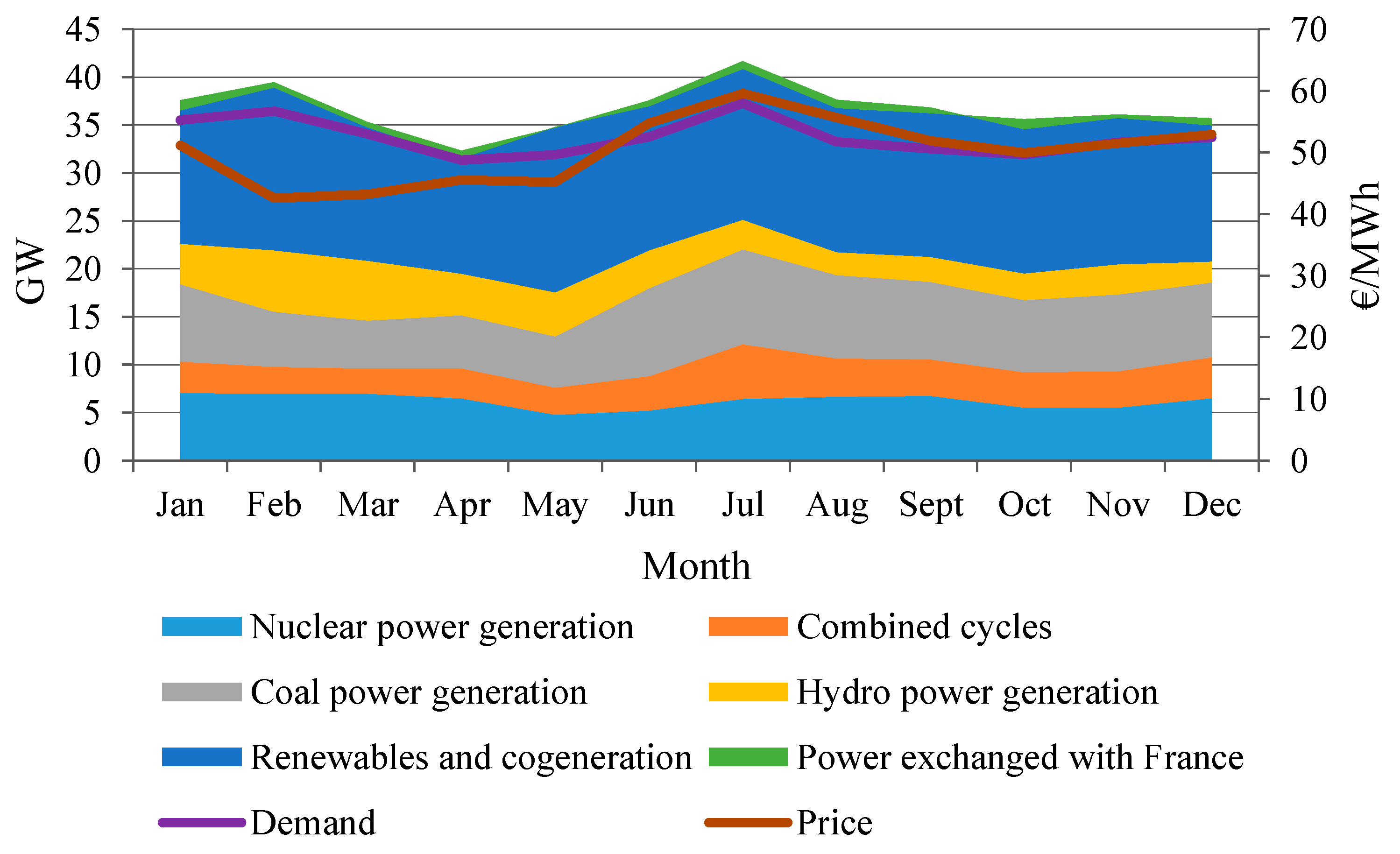
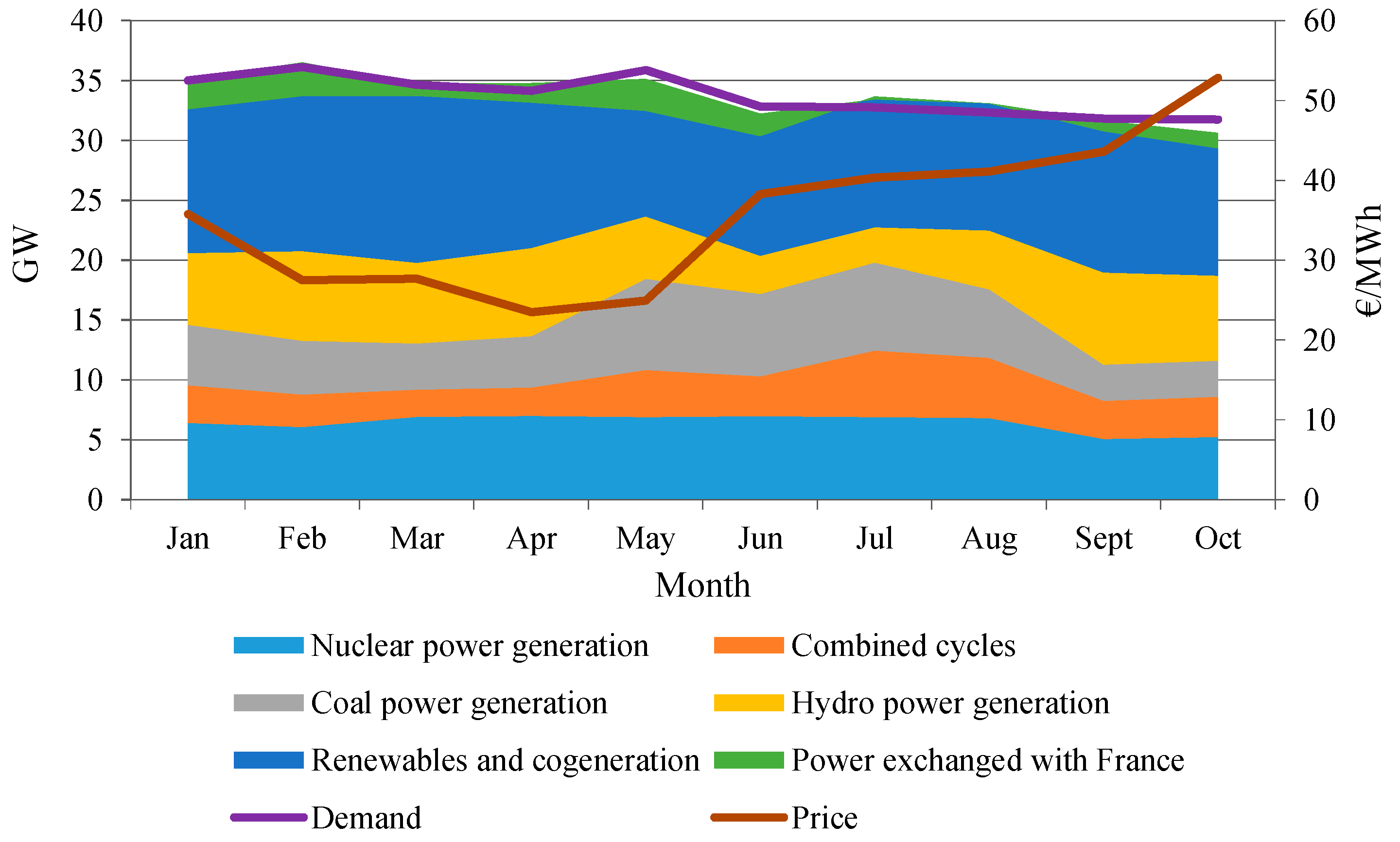
In order to understand the quality of predictor forecasts, an analysis of the values of historical data for the years 2015 and 2016 was carried out. Monthly electricity generation values, as well as the demand and real price of electricity values, corresponding to 2015 and to the first ten months of 2016 are plotted in Figure 1 and Figure 2, respectively.

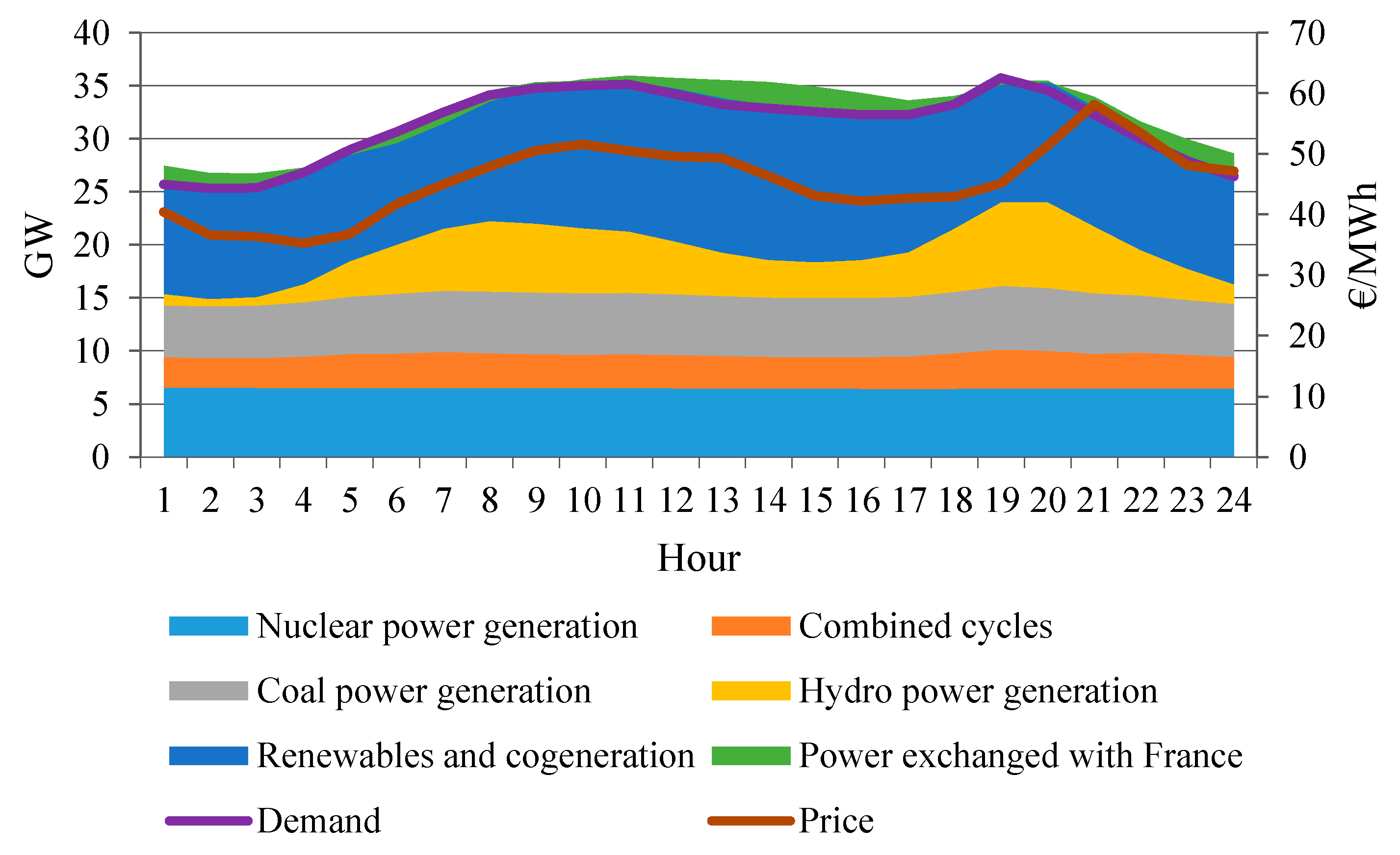
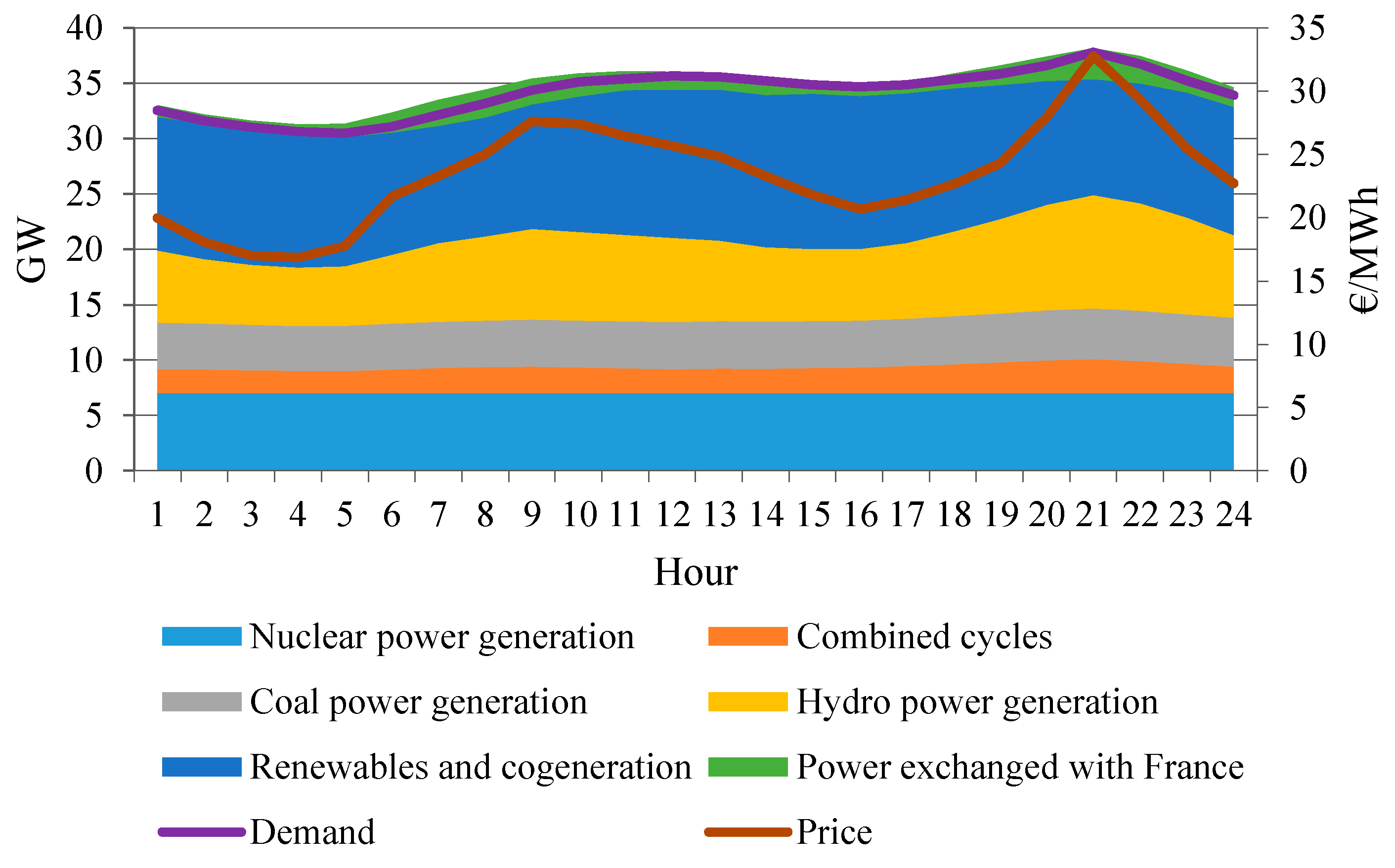
Both figures show the monthly average values of power demand, hydropower generation, renewable (wind and solar) and cogeneration power generation, coal power generation, nuclear power generation, combined cycle power generation and power exchanged with France. Monthly average electricity prices in the daily session of the MIBEL are also represented in both figures. Figure 3 and Figure 4 show hourly mean values of electricity generation through the most varied sources, demand and real price of electricity corresponding to April 2015 and April 2016, respectively.

As indicated in Figure 3 and Figure 4, the month of April 2015 shows quite significant changes compared to the same month in 2016 (shown in Figure 4). These are meaningful months in the production of electricity by the hydroelectric plants, which increased significantly in 2016 as a consequence of a higher rainfall than that of year 2015. As a result, the production of electricity by coal and natural gas power plants decreased, and the special regime production (where mini and micro-hydro productions are included) increased. All these facts led to a 40–50% decrease in electricity prices, which means that there was an increased difficulty in the price forecasting capabilities of the predictors of the for April 2016, due to the changes of generations with respect to those in April 2015.

2.3. Predictors Performance

The evaluation of the forecasts provided by the predictors of the EEM2016 EPF competition was mainly based on mean absolute errors expressed in €/MWh. The final rank of the EEM2016 EPF competition was computed after competition closure by calculating the hourly Mean Absolute Error for the best 10 days of forecast, for the entire 5 days forecast horizon. In spite of a better use of the limited number of forecast days of the competition, in this article we evaluate the performance of predictors for the 14 days of such competition, and thus maximizing the utilization of the available information.

In this article, the rank of predictors (from predictor P1 to predictor P20) was carried out for the day-ahead (D + 1) taking into account the forecasts provided by the competitors at day D, for a better analysis of the probabilistic price forecasting models presented later, in Section 3.

The mean absolute error MAE(D + k) corresponding to the forecast for day D + k (k = 1, 2, 3, 4, 5), provided at day D, is defined by Equation (1):

$$MAE\left(D+k\right)=\frac{1}{24}\times {\displaystyle \sum }_{h=1}^{24}\left|{\widehat{P}}_{D|\left(D+k\right)h}-P\left(D+k\right)h\right|$$

(1)

where ${\widehat{P}}_{D|\left(D+k\right)h}$ is the forecasted price (provided at day D) for hour h of day D + k, and $P\left(D+k\right)h$ is the real price for hour h of day D + k.

The predictors were globally ranked, from higher ranks to lower ranks, in the competition period, according to the MAE for “all days” of the competition period, $MA{E}_g\left(D+1\right)$, which corresponds to the average of the mean absolute errors for day D + 1 associated with the forecasts provided during the days of the competition period. $MA{E}_g\left(D+1\right)$ for all the competition period (14 days) is given by Equation (2):

$$MA{E}_g\left(D+1\right)=\frac{1}{24\times 14}·{\displaystyle \sum }_{D=1}^{14}{\displaystyle \sum }_{h=1}^{24}\left|{\widehat{P}}_{D|\left(D+1\right)h}-P\left(D+1\right)h\right|$$

(2)

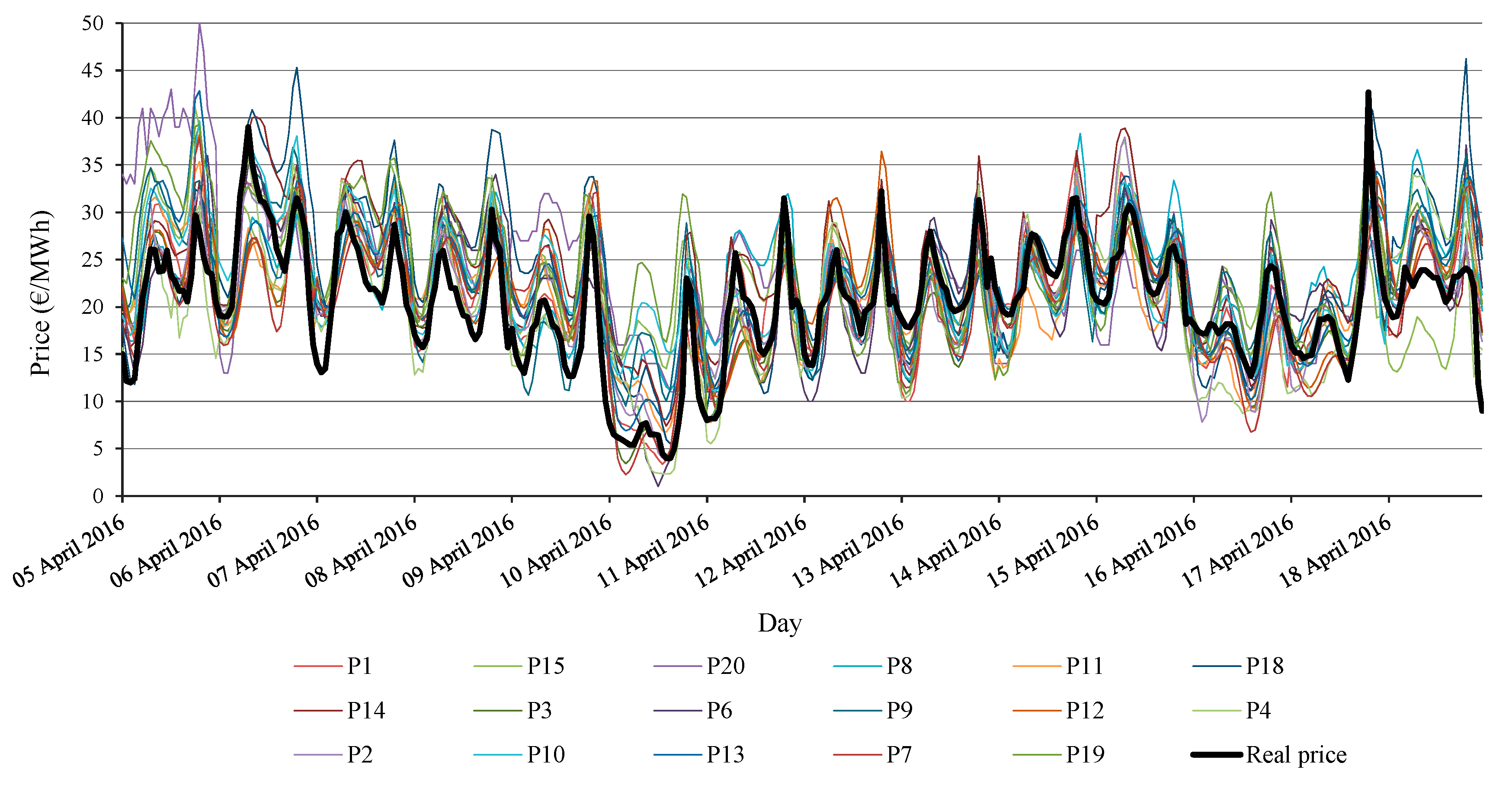
Figure 5 shows the forecasts ${\widehat{P}}_{D|\left(D+1\right)h}$ for the twenty best predictors (P1 to P20), provided by the competitors at day D for each hour h of day D + 1, during the days of competition in April 2016. Furthermore, the real price is also shown in Figure 5.

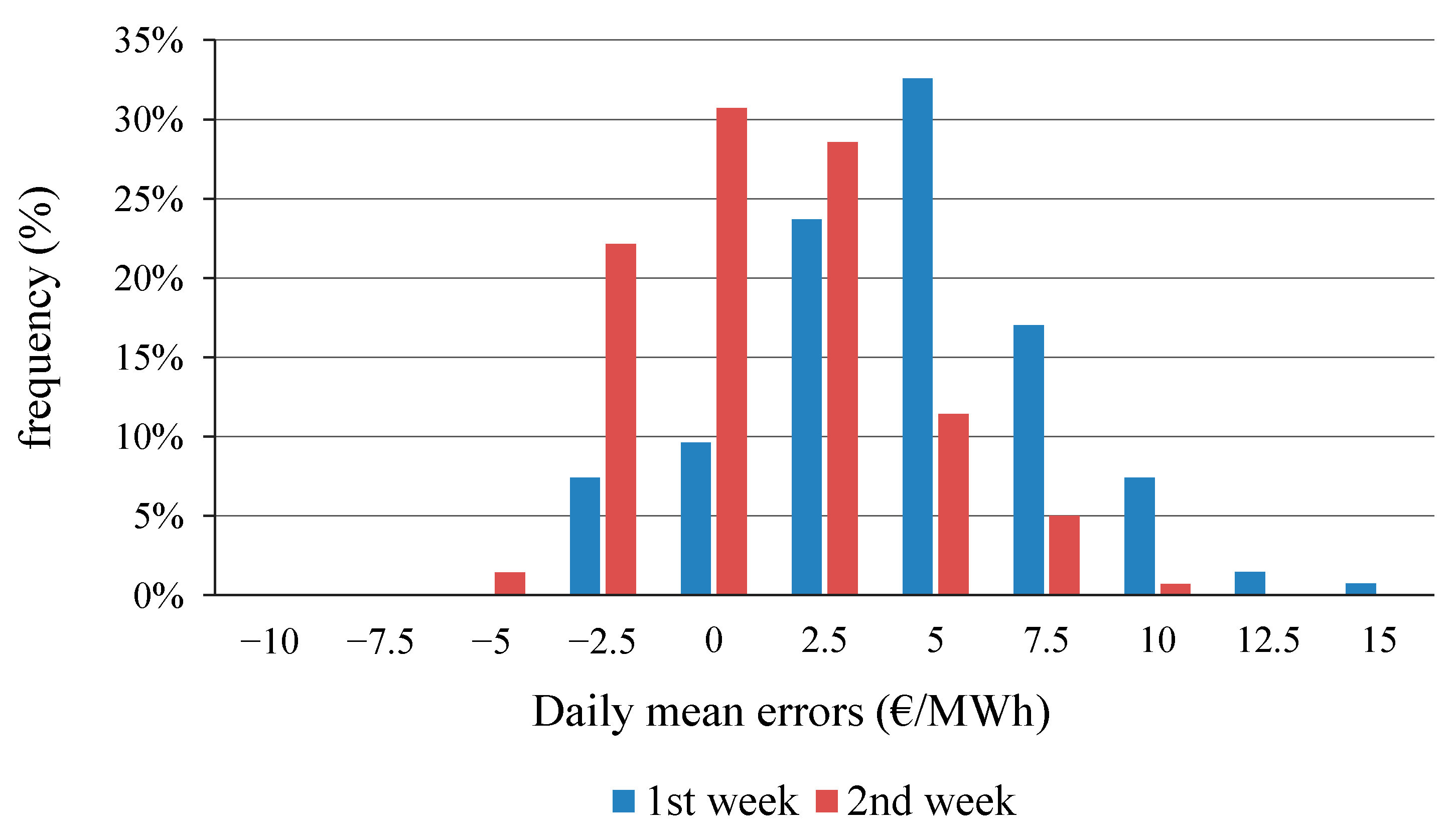
Figure 6 shows the histogram of daily mean errors of the price forecasts provided by the predictors for each of the two weeks of the competition, based on day-ahead hourly price forecasted values minus real hourly price values. Thus, the mentioned daily mean errors (for each predictor i) are calculated according to expression (3):

$$\frac{1}{24}{\displaystyle \sum }_{h=1}^{24}\left({\widehat{P}}_{i,D|\left(D+1\right)h}-P\left(D+1\right)h\right)$$

(3)

where, ${\widehat{P}}_{i,D|\left(D+1\right)h}$ is the price forecasted at day D for hour h of day D + 1 by the predictor i (point forecast, for hour h of day D + 1), and $P\left(D+1\right)h$ is the real price for hour h of day D + 1.

The average price during the competition period was 20.5 €/MWh, and the real price values ranged from 0 to 42.7 €/MWh. Observe that MAPE (mean absolute percentage error) corresponds to MAE divided by this average price during the competition period.

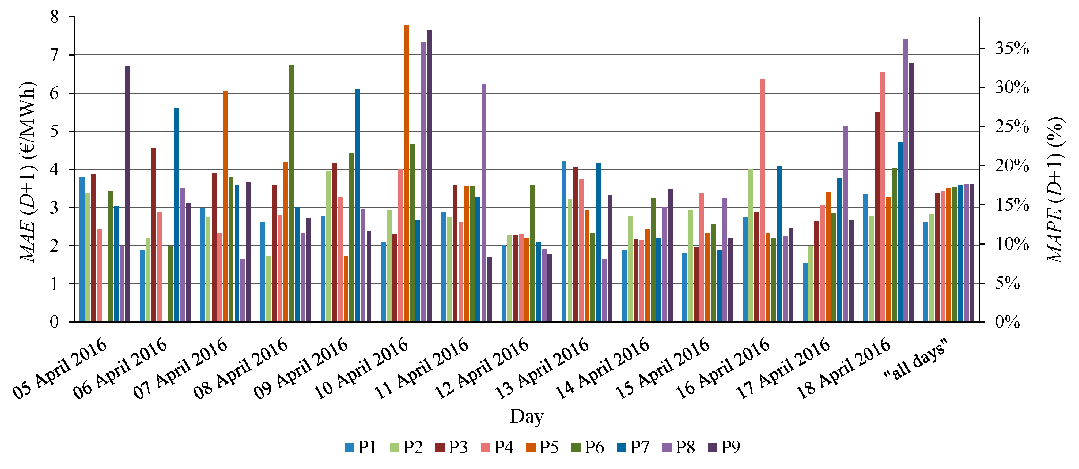
Figure 6 shows that the daily mean error with the highest frequency in the first week is around 5 (€/MWh), representing about 25% of the average price during the competition period. In general, the predictors forecasted price in excess, possibly caused by the exceptional weather conditions in the competition period, with more hydro and wind generation than those of the historical data used to build the predictors. In the first week of the competition, the bias was more significant than in the second week, indicating an improvement of the predictors’ performance during the competition. This element of improvement is also evident in Figure 7, with the exception of the 18 April 2016, with a high penetration of renewable generation. Figure 7 shows the values of MAE(D + 1) and MAPE(D + 1) for each day of the competition period as well as the values of $MA{E}_g\left(D+1\right)$, that is, MAE for “all days” of the competition period, of the nine best ranked predictors, P1 to P9. Observe that MAPE(D + 1) corresponds to MAE(D + 1) divided by the average price during the competition period.

The performances of the first and second best ranked predictors (P1 and P2) for “all days” of the competition period (with $MA{E}_g\left(D+1\right)$ of 2.6 and 2.8 €/MWh, respectively), are better than those of the third predictor, P3, and the remaining predictors (which have $MA{E}_g\left(D+1\right)$ around 3.5 €/MWh).

It should be noted that the EEM2016 EPF competition was a real rolling price forecast environment, with a total of forty four real predictors (SPF tools) and a large set of input data. Very limited information about predictors, and the data used by them, was available. However, we knew that predictors P1 and P2 were used by professional traders with access to privileged information and with high experience in electricity price markets. Predictors P3, P4 and P5 were utilized by academics who used only part of the public data available for the EEM2016 EPF competition and applied neural network modelling and advanced forecasting techniques. These facts are important to observe that predictors of the academics using limited information are not as good as the predictors of professional traders, but the forecasts of the predictors of the academics seem to be close to the forecasts of the best predictors.

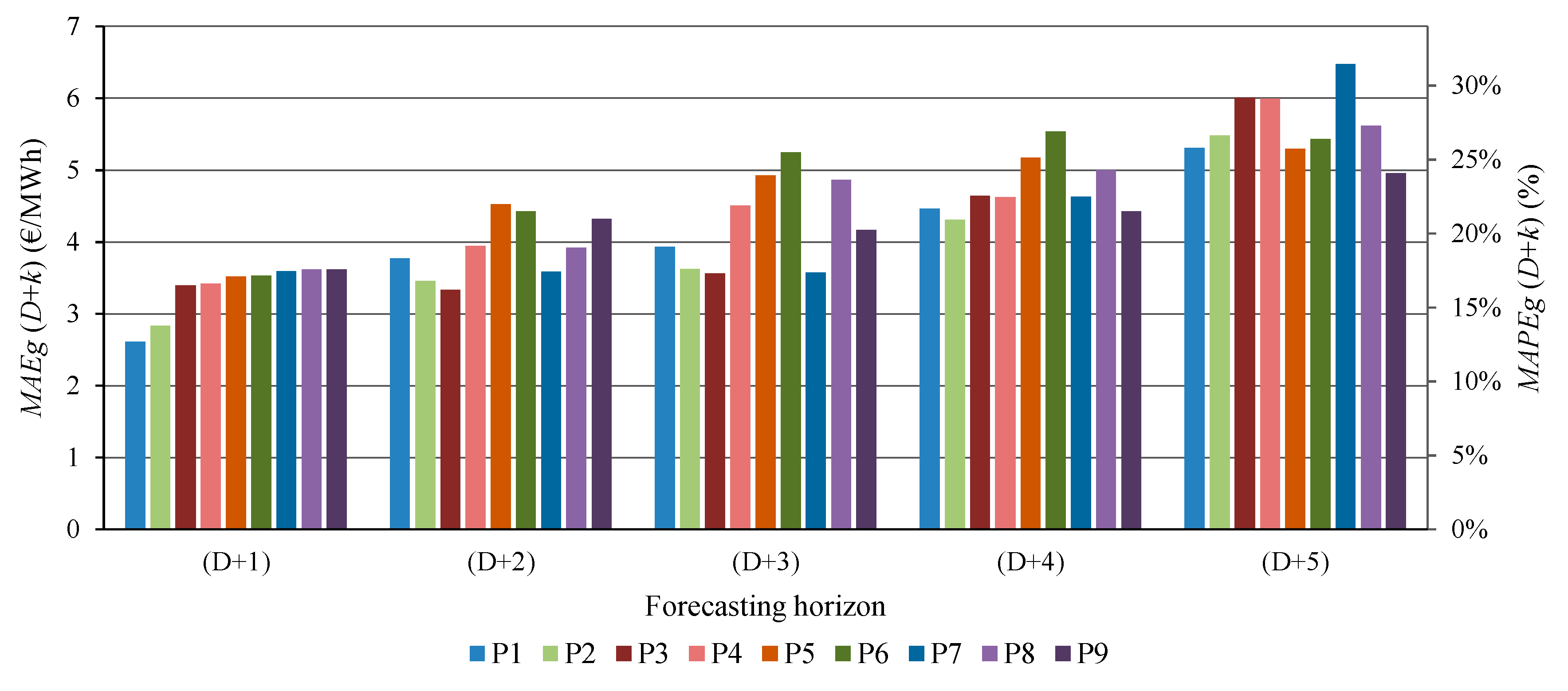
Figure 8 shows values of $MA{E}_g\left(D+1\right)$ to $MA{E}_g\left(D+5\right)$, as well as the corresponding values of $MAP{E}_g\left(D+1\right)$ to $MAP{E}_g\left(D+5\right)$, of the predictors P1 to P9, for day D + 1 to day D + 5, respectively, during the period of the competition, according to Equation (4) with (k = 1, 2, 3, 4, 5):

$$MA{E}_g\left(D+k\right)=\frac{1}{24\times 14}{\displaystyle \sum }_{D=1}^{14}{\displaystyle \sum }_{h=1}^{24}\left|{\widehat{P}}_{D|\left(D+k\right)h}-P\left(D+k\right)h\right|$$

(4)

The $MAP{E}_g\left(D+k\right)$ value corresponds to the $MA{E}_g\left(D+k\right)$ value divided by the average price value during the competition period.

Figure 8 shows an increase in the $MA{E}_g\left(D+k\right)$ error as k increased, that is, the performance of the forecast for the day D + k worsens as the considered day D + k is farther away from day D. The forecasts provided at day D for day D + k with k = 2 to 5 can be important for a forecast user when no new forecasts are available at the days following day D due to (for example) fails in technology supporting the communications between such forecast user and the forecast provider, or due to any kind of energy storage, which might need to know prices over the next few days to decide operation now. Figure 8 proves that forecast performances up to k = 5 have an acceptable quality and, therefore, the forecasts for k = 2 to 5 (at day D) could be considered for practical strategic decisions, especially when they are the only information available (i.e., due to fails in technology, as specified above). Furthermore, the price forecast for k = 2 to 5 can be useful for some decisions associated with short-term bidding strategies in electricity markets, as for example bidding in week-ahead future electricity derivative products.

In Figure 8 the increase of $MA{E}_g\left(D+k\right)$ values, with respect to those of $MA{E}_g\left(D+1\right)$, does not seem very significant for k = 2; but the increase of $MA{E}_g\left(D+k\right)$ values is evident for k = 5. It should be noted that the best predictors, P1 and P2, which are the best predictors according to MAE for “all” the competition period (that is, according to $MA{E}_g\left(D+1\right)$), are not always better than the other predictors from the point of view of $MA{E}_g\left(D+k\right)$ for k ≠ 1. For example, it can be observed that predictor P3 (academic competitor) is the best predictor for k = 2 and k = 3 from a point of view of $MA{E}_g\left(D+k\right)$.

3. Probabilistic Forecasting Models by Aggregation of Competitive Predictors

Forecasts of the predictors are point (spot) forecasts. Therefore, the ensemble of these predictor forecasts can be the basis for a probabilistic representation of the set of point forecasts by using probabilistic price forecasting models.

A detailed modelling of PDFs of Beta distributions for each hour of probabilistic price forecasts is first described in this Section 3, as well as two indicators of uncertainty of probabilistic forecasts. Afterwards three probabilistic price forecasting models (PPFMCP models) by aggregation of competitive predictors are presented in Section 3.1, Section 3.2 and Section 3.3.

Let’s say that point forecasts for hour h of day D + 1 of n predictors (forecasts provided at day D), are ${\widehat{P}}_{i,D|\left(D+1\right)h}$ (i = 1, 2,… n). Let’s say that the maximum forecasted price value for hour h of day D + 1 from the set of forecasts of n predictors is represented by $\underset{i}{\underbrace{max}}\left\{{\widehat{P}}_{i,D|\left(D+1\right)h}\right\}$; and let ’s say that the minimum forecasted price value for hour h of day D + 1 from the set of forecasts of n predictors is represented by $\underset{i}{\underbrace{min}}\left\{{\widehat{P}}_{i,D|\left(D+1\right)h}\right\}$. We can then obtain a PDF, ${\widehat{B}}_{D|\left(D+1\right)h}$, of a Beta distribution supported in the interval [$\underset{i}{\underbrace{min}}\left\{{\widehat{P}}_{i,D|\left(D+1\right)h}\right\}$; $\underset{i}{\underbrace{max}}\left\{{\widehat{P}}_{i,D|\left(D+1\right)h}\right\}$], corresponding to the stochastic price forecast variable ${\tilde{P}}_{D|\left(D+1\right)h}$. The PDF ${\widehat{B}}_{D|\left(D+1\right)h}$ is defined by four Beta distribution parameters: ${\alpha }_{D|\left(D+1\right)h}$; ${\beta }_{D|\left(D+1\right)h}$; $\underset{i}{\underbrace{min}}\left\{{\widehat{P}}_{i,D|\left(D+1\right)h}\right\}$ and $\underset{i}{\underbrace{max}}\left\{{\widehat{P}}_{i,D|\left(D+1\right)h}\right\}$ [55]. The parameters ${\alpha }_{D|\left(D+1\right)h}$ and ${\beta }_{D|\left(D+1\right)h}$ will be calculated further on (Equations (10) and (11)). Thus, ${\widehat{B}}_{D|\left(D+1\right)h}$ is represented by the function of expression (5):

$$f\left({\tilde{P}}_{D|\left(D+1\right)h};{\alpha }_{D|\left(D+1\right)h},{\beta }_{D|\left(D+1\right)h},\underset{i}{\underbrace{min}}\left\{{\widehat{P}}_{i,D|\left(D+1\right)h}\right\},\underset{i}{\underbrace{max}}\left\{{\widehat{P}}_{i,D|\left(D+1\right)h}\right\}\right)$$

(5)

A PDF, ${\widehat{B\prime }}_{D|\left(D+1\right)h}$, of a Beta distribution, supported in the interval [0, 1], corresponding to the normalized stochastic price forecast variable ${\widetilde{P\prime }}_{D|\left(D+1\right)h}$ can be defined. The stochastic normalized variable ${\widetilde{P\prime }}_{D|\left(D+1\right)h}$ is associated with normalized values ${\widehat{P\prime }}_{i,D|\left(D+1\right)h}$ which are defined by Equation (6):

$${\widehat{P\prime }}_{i,D|\left(D+1\right)h}=\frac{{\widehat{P}}_{i,D|\left(D+1\right)h}-\underset{i}{\underbrace{min}}\left\{{\widehat{P}}_{i,D|\left(D+1\right)h}\right\}}{\underset{i}{\underbrace{max}}\left\{{\widehat{P}}_{i,D|\left(D+1\right)h}\right\}-\underset{i}{\underbrace{min}}\left\{{\widehat{P}}_{i,D|\left(D+1\right)h}\right\}}$$

(6)

Thus, ${\widehat{B\prime }}_{D|\left(D+1\right)h}$ is represented by the function of expression (7):

$$f\prime \left({\widetilde{P\prime }}_{D|\left(D+1\right)h};{\alpha }_{D|\left(D+1\right)h},{\beta }_{D|\left(D+1\right)h}\right)$$

(7)

Parameters, ${\alpha }_{D|\left(D+1\right)h}$ and ${\beta }_{D|\left(D+1\right)h}$, can be obtained from the expected value $E\left[{\widehat{B\prime }}_{D|\left(D+1\right)h}\right]$ and the variance $V\left[{\widehat{B\prime }}_{D|\left(D+1\right)h}\right]$ of the ensemble of n normalized forecasted price values ${\widehat{P\prime }}_{i,D|\left(D+1\right)h}$ (i = 1, 2, … n) for hour $h$ of day D + 1, associated with the forecasted price values ${\widehat{P}}_{i,D|\left(D+1\right)h}$, provided at day D.

The expected value $E\left[{\widehat{B\prime }}_{D|\left(D+1\right)h}\right]$ and variance $V\left[{\widehat{B\prime }}_{D|\left(D+1\right)h}\right]$ are determined by Equations (8) and (9), respectively:

$$E\left[{\widehat{B\prime }}_{D|\left(D+1\right)h}\right]=\frac{{{\displaystyle \sum }}_{i=1}^n\left({\widehat{P\prime }}_{i,D|\left(D+1\right)h}·w_{i,D}\right)}{{{\displaystyle \sum }}_{i=1}^n{w}_{i,D}}$$

(8)

$$V\left[{\widehat{B\prime }}_{D|\left(D+1\right)h}\right]=\frac{{{\displaystyle \sum }}_{i=1}^n\left({\left({\widehat{P\prime }}_{i,D|\left(D+1\right)h}\right)}^2·w_{i,D}\right)}{{{\displaystyle \sum }}_{i=1}^n{w}_{i,D}}-{\left(E\left[{\widehat{B^{\prime }}}_{D|\left(D+1\right)h}\right]\right)}^2$$

(9)

where $w_{i,D}$ is a weight value for predictor i at day D that depends on the model chosen among the probabilistic price forecasting models that are presented in Section 3.1, Section 3.2 and Section 3.3.

With the expected value $E\left[{\widehat{B\prime }}_{D|\left(D+1\right)h}\right]$ and variance $V\left[{\widehat{B\prime }}_{D|\left(D+1\right)h}\right]$, obtained by (8) and (9), parameters ${\alpha }_{D|\left(D+1\right)h}$ and ${\beta }_{D|\left(D+1\right)h}$ are calculated by Equations (10) and (11):

$${\alpha }_{D|\left(D+1\right)h}=\frac{\left(1-E\left[{\widehat{B\prime }}_{D|\left(D+1\right)h}\right]\right)·{\left(E\left[{\widehat{B^{\prime }}}_{D|\left(D+1\right)h}\right]\right)}^2}{V\left[{\widehat{B\prime }}_{D|\left(D+1\right)h}\right]}-E\left[{\widehat{B\prime }}_{D|\left(D+1\right)h}\right]$$

(10)

$${\beta }_{D|\left(D+1\right)h}{=}_{D|\left(D+1\right)h}·\frac{1-E\left[{\widehat{B\prime }}_{D|\left(D+1\right)h}\right]}{E\left[{\widehat{B\prime }}_{D|\left(D+1\right)h}\right]}$$

(11)

Three probabilistic price forecasting models are going to be presented further on in this article (Section 3.1, Section 3.2 and Section 3.3), which are:

• Probabilistic price forecasting model 1 (PPFMCP model 1) by aggregation of competitive predictors: PPFMCP model 1 uses aggregation by the averaging of price predictor forecasts and it is commented in Section 3.1.
• Probabilistic price forecasting model 2 (PPFMCP model 2) by aggregation of competitive predictors: PPFMCP model 2 utilizes aggregation of price predictor forecasts by means of weight values according to a daily rank of the predictors and it is explained in Section 3.2.
• Probabilistic price forecasting model 3 (PPFMCP model 3) by aggregation of competitive predictors: PPFMCP model 3 uses aggregation by means of optimized weights and it is described in Section 3.3.

Then, the expected value of the hourly price (point forecast of hourly price value) of each PPFMCP model, with price values expressed in €/MWh in interval [$\underset{i}{\underbrace{min}}\left\{{\widehat{P}}_{i,D|\left(D+1\right)h}\right\}$; $\underset{i}{\underbrace{max}}\left\{{\widehat{P}}_{i,D|\left(D+1\right)h}\right\}$], can be obtained by using the PDF given by expression (5) of a Beta distribution, supported in such interval. Thus, the expected value of the hourly price is given by expression (12).

$$\underset{i}{\underbrace{min}}\left\{{\widehat{P}}_{i,D|\left(D+1\right)h}\right\}+\left(\underset{i}{\underbrace{max}}\left\{{\widehat{P}}_{i,D|\left(D+1\right)h}\right\}-\underset{i}{\underbrace{min}}\left\{{\widehat{P}}_{i,D|\left(D+1\right)h}\right\}\right)·\left(\frac{{\alpha }_{D|\left(D+1\right)h}}{{\alpha }_{D|\left(D+1\right)h}+{\beta }_{D|\left(D+1\right)h}}\right)$$

(12)

Practical probabilistic values of each PPFMCP model can be also obtained from their PDF given by expression (5). These probabilistic models can then lead to the evaluation of risk decisions based on price, calculations on the probability to have prices which are higher than some price limits, calculations on the probability to obtain prices in a target interval, calculations of quantiles, etc. For example, quantile $Q_{p;D|\left(D+1\right)h}$ for probability value $p$ can be obtained by using the inverse of the cumulative distribution function (represented by $C{F}^{-1}$) for function ${\widehat{B}}_{D|\left(D+1\right)h}$, through expression (13):

$$C{F}^{-1}\left(p;\underset{i}{{\alpha }_{D|\left(D+1\right)h},{\beta }_{D|\left(D+1\right)h}, \underbrace{min}}\left\{{\widehat{P}}_{i,D|\left(D+1\right)h}\right\},\underset{i}{\underbrace{max}}\left\{{\widehat{P}}_{i,D|\left(D+1\right)h}\right\}\right)$$

(13)

On one hand, appropriate performance error indicators, as the mean absolute error, can be used to evaluate the accuracy of explainable information of the forecasts of the PPFMCP models, based on deviations in real price values with respect to the expected values of the hourly price (point forecast of hourly price) from such PPFMCP models.

On the other hand, the accuracy of representing the non-explainable information of the forecasts of the PPFMCP models can be evaluated by suitable indicators of uncertainty of the probabilistic forecasts of such models. Two indicators of probabilistic price forecast uncertainty of the probabilistic models have been introduced in this article, which are the Loss function Indicator, LI, and the Reliability Indicator, RI, described in the following paragraphs.

Indicator LI depends on vector $\overleftrightarrow{B}$ (that is, $I\left(\overleftrightarrow{B}\right)$). Vector $\overleftrightarrow{B}$ contains m probabilistic forecasts (of a considered PPFMCP model) for a given period. For the EEM 2016 EPF competition, m is associated with the 312 h of the period between the 6th and the 18th of April 2016, totalizing 312 probabilistic price forecasts ${\widehat{B}}_t$, (t = 1, 2, 3,….. 312). It should be noted that index t corresponds to hour h of day D + 1 during the mentioned period. Indicator LI takes each quantile $Q_{p,t}$ into account for each probability $p$ and for each hour $t$ of the forecasts, as well as vector $\overleftrightarrow{B}$ which contains all the probabilistic forecasts (${\widehat{B}}_t$).

Indicator LI is calculated by evaluating quantile deviations with respect to the real price for each hour t. Here, the real price is represented as P_t. Observe that P_t corresponds to P(D + 1)h of Equation (2), (i.e., $P\left(D+1\right)h$ is the real price for hour h of day D + 1). Thus, the quantile derivations $L\left(Q_{p,t};P_t\right)$ are obtained by Equation (14):

$$L\left(Q_{p,t};P_t\right)=\{\begin{array}{c}\left(P_t-Q_{p;t}\right)·p\\ \left(Q_{p;t}-P_t\right)·\left(1-p\right)\end{array}\begin{array}{c}if P_t\ge Q_{p;t}\\ if P_t<Q_{p;t}\end{array}$$

(14)

where quantile $Q_{p,t}$ is obtained according to expression (13). It should be noted that $Q_{p,t}$ corresponds to $Q_{p;D|\left(D+1\right)h}$ during the abovementioned period.

The Loss function Indicator, LI, is then computed by Equation (15) and corresponds to the average value of the quantile derivations (relatively to the real price) for the total of $nq$ quantiles and the total of m hours:

$$LI=\frac{1}{m\times nq}·{\displaystyle \sum }_{t=1}^m{\displaystyle \sum }_{p=\frac{1}{nq+1}}^{\frac{nq}{nq+1}}L\left(Q_{p,t};P_t\right)$$

(15)

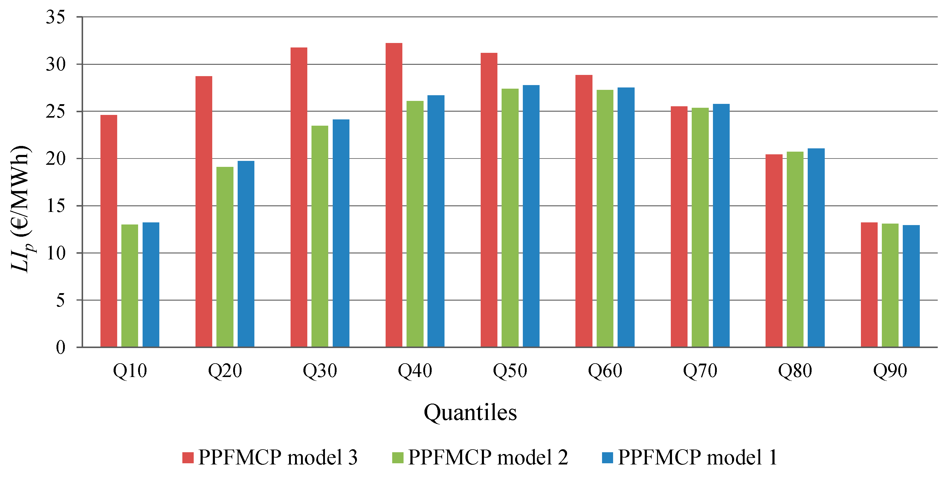
The accuracy of representing the non-explainable information of the forecasts of a PPFMCP model is better for lower values of LI. Indicator LI corresponds to a unique value which allows to make the comparison among PPFMCP models. However, this does not allow to carry out a detailed analysis. The Loss function Indicator for each quantile, LI_p, can be used for a graphic representation and analysis, as shown in Section 4. LI_p is computed by Equation (16):

$$L{I}_p=\frac{1}{m}·{\displaystyle \sum }_{t=1}^{m}L\left(Q_{p,t};P_t\right)$$

(16)

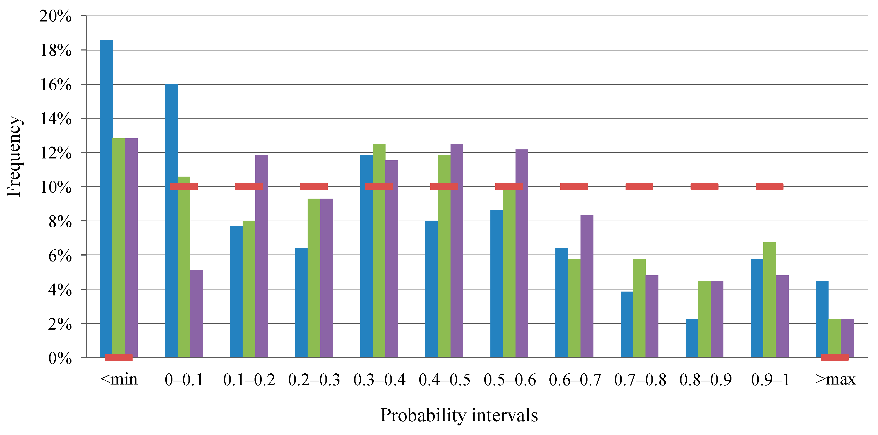
In order to calculate the Reliability Indicator, RI, some previous definitions are necessary. A reliability diagram can be obtained for the probabilistic hourly price forecasts of each PPFMCP model, as shown later in Section 4. In the horizontal axis of the diagram, probability intervals ($pi$) are represented. The number of probability intervals $npi$ are defined in accordance with the desired degree of detail and with the number $m$ of forecasts available for evaluation. Probability interval $pi$ corresponds to the interval defined by the quantile for probability $p_{\left(pi-1\right)}$ and by the quantile for probability $p_{\left(pi\right)}$, where $(p_{\left(pi\right)}-p_{\left(pi-1\right)})$ is constant.

In the vertical axis of the reliability diagram, the frequency of the events (price occurrences) are represented. The target frequency is an ideal frequency of events, (100 × ftar_pi), as a percentage, which can be calculated as 100 divided by the $npi$ number. Furthermore, in such vertical axis the observed frequency, (100 × fobs_pi), as a percentage, corresponds to the frequency of the events (price occurrences) consisting in that the real price value P_t occurs into the considered probability interval $pi$, that is, P_t is greater than (or equal to) the quantile for probability $p_{\left(pi-1\right)}$ for hour t and P_t is lower than the quantile for probability $p_{\left(pi\right)}$ for hour t.

For cases when value P_t occurs outside the limits of the PDF of the Beta distribution for hour t (value lower than the minimum, or value greater than maximum from the set of predictors), fobs_pi frequencies are also computed. It is necessary to observe that ftar_pi frequencies are zero when the values of real price occur outside those limits, which corresponds to events occurring into two additional “intervals” (indication “˂min” for interval below the minimum, and indication “>max” for interval above the maximum).

Reliability Indicator RI, as a percentage, is computed by Equation (17):

$$RI=\left(1-{\displaystyle \sum }_{pi=1}^{npi+2}\left|fob{s}_{pi}-fta{r}_{pi}\right|\right)\times 100$$

(17)

where $pi=npi+1$ is associated with indication “˂min” (ftar_pi = 0), and $pi=npi+2$ is associated with indication “˃max” (ftar_pi = 0).

Higher values of RI indicate a better accuracy for representing the non-explainable information of the forecasts of the PPFMCP models, that is, a better matching of the PDFs during the abovementioned period. Indicator RI returns a unique value for each probabilistic model; however, it is possible to evaluate details of the adequacy quality of the PDFs by observing the reliability diagram and by analyzing the frequencies of events in each probability interval.

3.1. Probabilistic Price Forecasting Model 1 (PPFMCP Model 1) by Aggregation of Competitive Predictors

PPFMCP model 1 uses the averaging of the price forecasts of the predictors. PPFMCP model 1 uses unitary weights $(w_{i,D}=1)$ in Equations (8) and (9) for the twenty best predictors (P1 to P20), being n = 20. Values of parameters ${\alpha }_{D|\left(D+1\right)h}$ and ${\beta }_{D|\left(D+1\right)h}$ are then obtained by Equations (10) and (11).

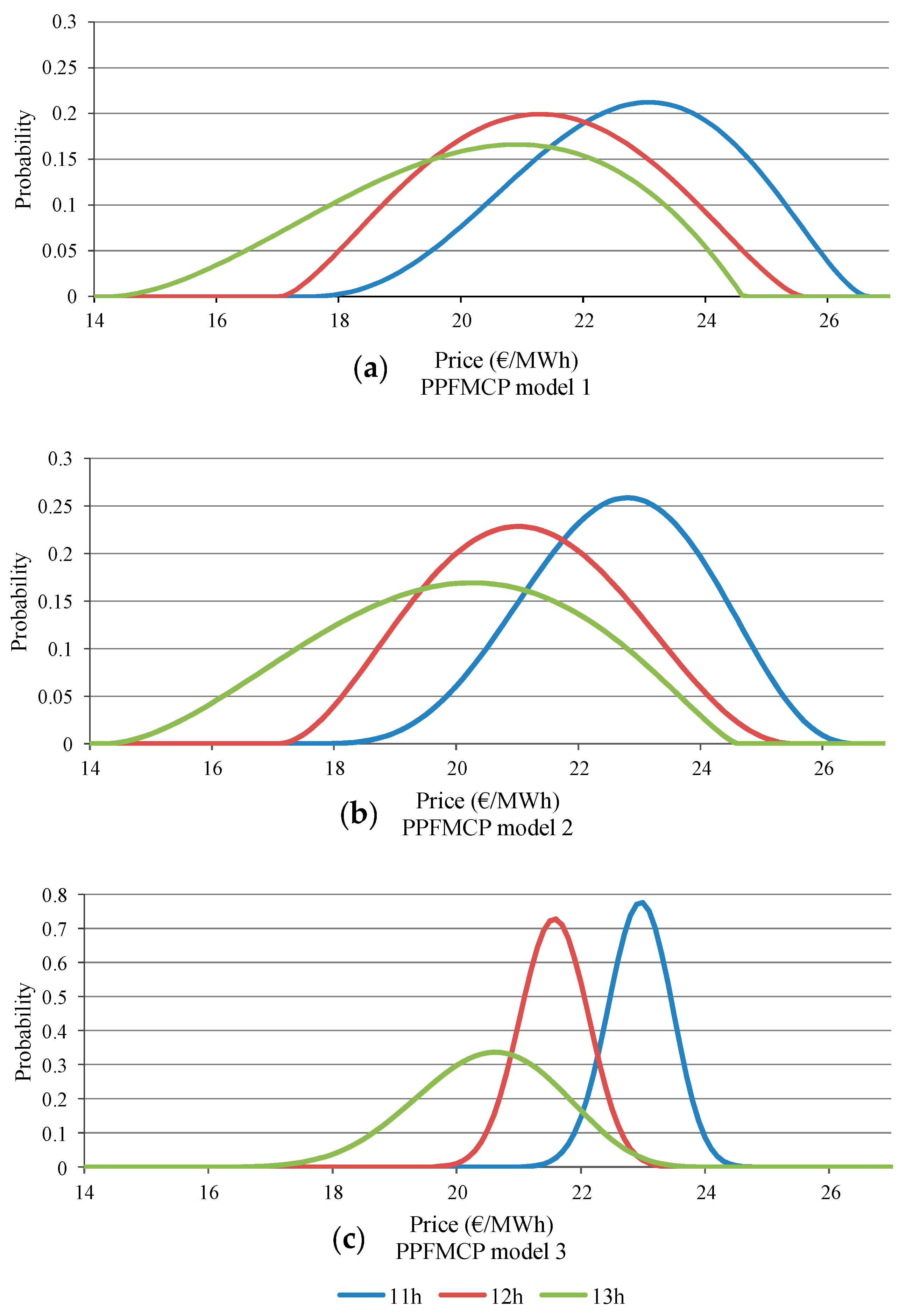
Probabilistic price forecasts of PPFMCP model 1 correspond to PDFs of Beta distributions, with four parameters given by expression (5), for each hour h of day D + 1.

Table 1. Results of PPFMCP model 1.

Hour	Min Price (€/MWh)	Max Price (€/MWh)	${\mathit{\alpha }}_{\mathit{D}|\left(\mathit{D}+1\right)\mathit{h}}$	${\mathit{\beta }}_{\mathit{D}|\left(\mathit{D}+1\right)\mathit{h}}$
11 h	17.40	26.67	3.63	2.67
12 h	17.06	25.61	2.50	2.53
13 h	14.23	24.62	2.83	2.01

and Figure 9a show examples of the results of PPFMCP model 1 for three hours, which are hours 11 h, 12 h, and 13 h, on the 14th of April, 2016. Table 1, for the three hours, shows values of $\underset{i}{\underbrace{min}}\left\{{\widehat{P}}_{i,D|\left(D+1\right)h}\right\}$ under column “Min Price (€/MWh)” and values of $\underset{i}{\underbrace{max}}\left\{{\widehat{P}}_{i,D|\left(D+1\right)h}\right\}$ under column “Max Price (€/MWh)”.

The three probability density functions of PPFMCP model 1, presented in Figure 9a, show different shapes for the three hours.

3.2. Probabilistic Price Forecasting Model 2 (PPFMCP Model 2) by Aggregation of Competitive Predictors

PPFMCP model 2 weights the different predictors as a function of a daily rank of each predictor. Rank $R_{i,D}$ is defined as the daily rank of predictor i at day D. $R_{i,D}$ is obtained taking into account a daily value of the mean absolute error of each predictor i for day D, which is calculated by expression (18):

$$\frac{1}{24}\times {\displaystyle \sum }_{h=1}^{24}\left|{\widehat{P}}_{i,\left(D-1\right)|\left(D\right)h}-P\left(D\right)h\right|$$

(18)

where ${\widehat{P}}_{i,\left(D-1\right)|\left(D\right)h}$ is the price forecasted by predictor i, at day D − 1 for hour h of day D, and $P\left(D\right)h$ is the real price for hour h of day D. It is important to observe that the price forecasts (set of ${\widehat{P}}_{i,\left(D-1\right)|\left(D\right)h}$) for day D are provided at day D − 1, and the real prices of day D (set of $P\left(D\right)h$) are also known at day D.

Daily rank $R_{i,D}$ is an integer number with values between 1 for the best predictor (P1), and 20 for the worst predictor (P20) of the 20 predictors. The inverse of rank $R_{i,D}$ of predictor $i$ (i = 1, 2, … 20) defines weight $w_{i,D}$ which is used by PPFMCP model 2 to forecast prices for day D + 1. That is, $w_{i,D}$ is (1/$R_{i,D}$) for PPFMCP model 2.

Weight values $w_{i,D}$ are then values that belong to the set {1, 1/2, 1/3, 1/4, 1/5…1/20}, taking into account the daily ranking of predictors. A vector of twenty weights was used (one weight value for each predictor), for each day D. In PPFMCP model 2, these weights were applied to Equations (8) and (9) for the twenty best predictors (P1 to P20), being n = 20.

Table 2. Weights w_i,D of the PPFMCP model 2 for the predictors P1 to P20.

Date	Predictors
	P1	P15	P20	P8	P11	P18	P14	P3	P6	P9	P12	P5	P17	P4	P2	P10	P16	P13	P7	P19
5 April 2016	0.14	0.07	0.06	1.00	0.09	0.50	0.25	0.10	0.13	0.08	0.11	0.06	0.05	0.33	0.17	0.08	0.05	0.07	0.20	0.06
6 April 2016	1.00	0.08	0.17	0.13	0.08	0.05	0.07	0.06	0.33	0.14	0.06	0.05	0.10	0.20	0.25	0.11	0.07	0.09	0.06	0.50
7 April 2016	0.25	0.06	0.20	1.00	0.08	0.05	0.06	0.10	0.11	0.13	0.09	0.06	0.07	0.50	0.33	0.07	0.14	0.08	0.17	0.05
8 April 2016	0.25	0.08	0.09	0.33	0.07	0.05	0.07	0.11	0.05	0.20	0.50	0.08	0.06	0.17	1.00	0.10	0.06	0.13	0.14	0.06
9 April 2016	0.33	0.09	0.05	0.25	0.10	0.05	0.07	0.14	0.11	0.50	0.06	1.00	0.08	0.20	0.17	0.08	0.06	0.07	0.06	0.13
10 April 2016	1.00	0.06	0.06	0.08	0.17	0.11	0.08	0.50	0.10	0.07	0.33	0.07	0.05	0.13	0.20	0.06	0.09	0.14	0.25	0.05
11 April 2016	0.13	0.06	0.05	0.05	0.08	0.25	0.06	0.07	0.08	0.50	0.06	0.07	0.11	0.20	0.17	0.33	1.00	0.14	0.09	0.10
12 April 2016	0.14	0.06	0.33	0.17	0.20	0.25	0.07	0.09	0.05	0.50	0.05	0.11	0.07	0.08	0.08	1.00	0.10	0.06	0.13	0.06
13 April 2016	0.05	1.00	0.11	0.50	0.14	0.33	0.13	0.06	0.20	0.08	0.07	0.10	0.17	0.06	0.08	0.09	0.25	0.07	0.06	0.05
14 April 2016	0.50	0.09	0.06	0.08	0.05	0.17	0.13	0.25	0.08	0.06	0.07	0.14	0.06	0.33	0.11	0.07	0.05	1.00	0.20	0.10
15 April 2016	0.50	1.00	0.05	0.06	0.08	0.17	0.05	0.20	0.09	0.14	0.10	0.11	0.06	0.06	0.07	0.08	0.07	0.13	0.25	0.33
16 April 2016	0.09	0.06	0.11	0.25	0.08	0.17	0.50	0.08	0.33	0.13	0.07	0.14	0.10	0.05	0.06	1.00	0.05	0.20	0.06	0.07
17 April 2016	1.00	0.20	0.09	0.05	0.08	0.06	0.07	0.17	0.13	0.14	0.08	0.07	0.06	0.10	0.33	0.50	0.05	0.11	0.06	0.25
18 April 2016	0.20	0.07	0.50	0.05	0.10	0.05	0.17	0.07	0.11	0.06	0.08	0.33	0.25	0.06	1.00	0.14	0.13	0.06	0.09	0.08

shows weights $w_{i,D}$ of PPFMCP model 2 for each predictor. As expected, the best daily performing predictors have higher weights values (more green cells and less red cells in Table 2).

Examples of the results for PPFMCP model 2 are presented in

Table 3. Results of PPFMCP model 2.

Hour	Min Price (€/MWh)	Max Price (€/MWh)	${\mathit{\alpha }}_{\mathit{D}|\left(\mathit{D}+1\right)\mathit{h}}$	${\mathit{\beta }}_{\mathit{D}|\left(\mathit{D}+1\right)\mathit{h}}$
11 h	17.40	26.67	5.26	4.04
12 h	17.06	25.61	3.06	3.39
13 h	14.23	24.62	2.87	2.35

and Figure 9b, for hours 11 h, 12 h, and 13 h on 14 April, 2016. PPFMCP model 2 leads to some more sharpened probability density distributions with respect to those from PPFMCP model 1. The effect of the higher sharpness of the probability density distributions obtained with PPFMCP model 2 is a bit more evident in hour 11 h.

3.3. Probabilistic Price Forecasting Model 3 (PPFMCP Model 3) by Aggregation of Competitive Predictors

The third probabilistic model, PPFMCP model 3, uses weights $u_{i,D}$ obtained by a minimization process for day D, which is defined by expression (19):

$$\begin{array}{l}\underset{by u_{i,D}}{\underbrace{minimize}}\left[{\displaystyle \sum }_{h=1}^{24}{\left({\displaystyle \sum }_{i=1}^n{u}_{i,D}·{\widehat{P}}_{i,\left(D-1\right)|\left(D\right)h}-P_{\left(D\right)h}\right)}^2\right]\\ \mathrm{subject}\mathrm{to}:0\le u_{i,D}\le 1, and {\displaystyle \sum }_{i=1}^n{u}_{i,D}=1\end{array}$$

(19)

In PPFMCP model 3, these weights $u_{i,D}$ are applied to Equations (8) and (9) ($u_{i,D}$ is used in substitution of $w_{i,D}$), for the twenty best predictors (P1 to P20), being n = 20. The results of the optimization of expression (19) depend on the differences in the performance of the predictors. In the EEM2016 EPF competition, there were significant differences in the performance of predictors.

Table 4. Weights u_i,D of the PPFMCP model 3 for the predictors P1 to P20.

Date	Predictors
	P1	P15	P20	P8	P11	P18	P14	P3	P6	P9	P12	P5	P17	P4	P2	P10	P16	P13	P7	P19
5 April 2016	0.00	0.00	0.00	0.00	0.00	0.23	0.48	0.00	0.00	0.03	0.00	0.04	0.03	0.14	0.00	0.01	0.03	0.00	0.00	0.00
6 April 2016	0.00	0.00	0.01	0.00	0.00	0.00	0.13	0.00	0.43	0.00	0.00	0.00	0.00	0.44	0.00	0.00	0.00	0.00	0.00	0.00
7 April 2016	0.00	0.00	0.00	0.78	0.00	0.00	0.00	0.00	0.00	0.00	0.00	0.00	0.00	0.21	0.01	0.00	0.00	0.00	0.00	0.00
8 April 2016	0.00	0.00	0.00	0.00	0.00	0.00	0.00	0.00	0.00	0.00	0.06	0.00	0.00	0.10	0.83	0.00	0.00	0.00	0.00	0.00
9 April 2016	0.00	0.00	0.00	0.00	0.00	0.00	0.00	0.00	0.00	0.36	0.00	0.64	0.00	0.00	0.00	0.00	0.00	0.00	0.00	0.00
10 April 2016	0.47	0.00	0.00	0.00	0.11	0.00	0.00	0.00	0.00	0.00	0.43	0.00	0.00	0.00	0.00	0.00	0.00	0.00	0.00	0.00
11 April 2016	0.00	0.17	0.00	0.00	0.00	0.20	0.00	0.00	0.00	0.05	0.00	0.18	0.00	0.41	0.00	0.00	0.00	0.00	0.00	0.00
12 April 2016	0.00	0.01	0.04	0.00	0.00	0.00	0.18	0.00	0.29	0.00	0.00	0.00	0.00	0.04	0.09	0.00	0.00	0.35	0.00	0.00
13 April 2016	0.00	0.32	0.00	0.47	0.00	0.00	0.00	0.00	0.19	0.00	0.00	0.00	0.00	0.00	0.02	0.00	0.00	0.00	0.00	0.00
14 April 2016	0.34	0.00	0.00	0.00	0.00	0.06	0.00	0.00	0.00	0.00	0.00	0.00	0.09	0.00	0.00	0.00	0.00	0.46	0.00	0.06
15 April 2016	0.01	0.00	0.00	0.00	0.00	0.16	0.00	0.00	0.11	0.02	0.00	0.09	0.11	0.00	0.00	0.00	0.00	0.03	0.26	0.22
16 April 2016	0.00	0.23	0.00	0.00	0.31	0.00	0.00	0.00	0.00	0.00	0.10	0.16	0.00	0.00	0.00	0.00	0.00	0.00	0.08	0.12
17 April 2016	0.00	0.00	0.00	0.00	0.00	0.00	0.06	0.00	0.28	0.00	0.00	0.00	0.00	0.30	0.00	0.23	0.00	0.00	0.00	0.13
18 April 2016	0.00	0.39	0.00	0.00	0.00	0.00	0.00	0.00	0.00	0.00	0.00	0.00	0.00	0.21	0.40	0.00	0.00	0.00	0.00	0.00

shows the weights values of $u_{i,D}$ of PPFMCP model 3 for the twenty best predictors (P1 to P20), where higher values are shown in green cells and null values are shown in red cells. In comparison with Table 2, now Table 4 shows that the optimization leads to select weights in a way that only a few predictors (in comparison with PPFMCP model 2) are used by PPFMCP model 3 for the day-ahead price forecasts. PPFMCP model 3 leads then to provide more sharpened PDFs than PPFMCP model 2.

In comparison with PPFMCP model 2, PPFMCP model 3 differentiates predictors, giving more relevance to predictors with a better performance.

Examples of results of PPFMCP model 3 are shown in

Table 5. Results of PPFMCP model 3.

Hour	Min Price (€/MWh)	Max Price (€/MWh)	${\mathit{\alpha }}_{\mathit{D}|\left(\mathit{D}+1\right)\mathit{h}}$	${\mathit{\beta }}_{\mathit{D}|\left(\mathit{D}+1\right)\mathit{h}}$
11 h	17.40	26.67	47.16	31.70
12 h	17.06	25.61	32.32	28.95
13 h	14.23	24.62	11.27	7.42

and Figure 9c for hours 11 h, 12 h, and 13 h on the 14th of April, 2016. In Figure 9c, the higher sharpness of the probability density functions obtained by PPFMCP model 3 is more evident compared with those of PPFMCP model 2 and PPFMCP model 1.

4. Analysis of Results of Probabilistic Price Forecasting Models

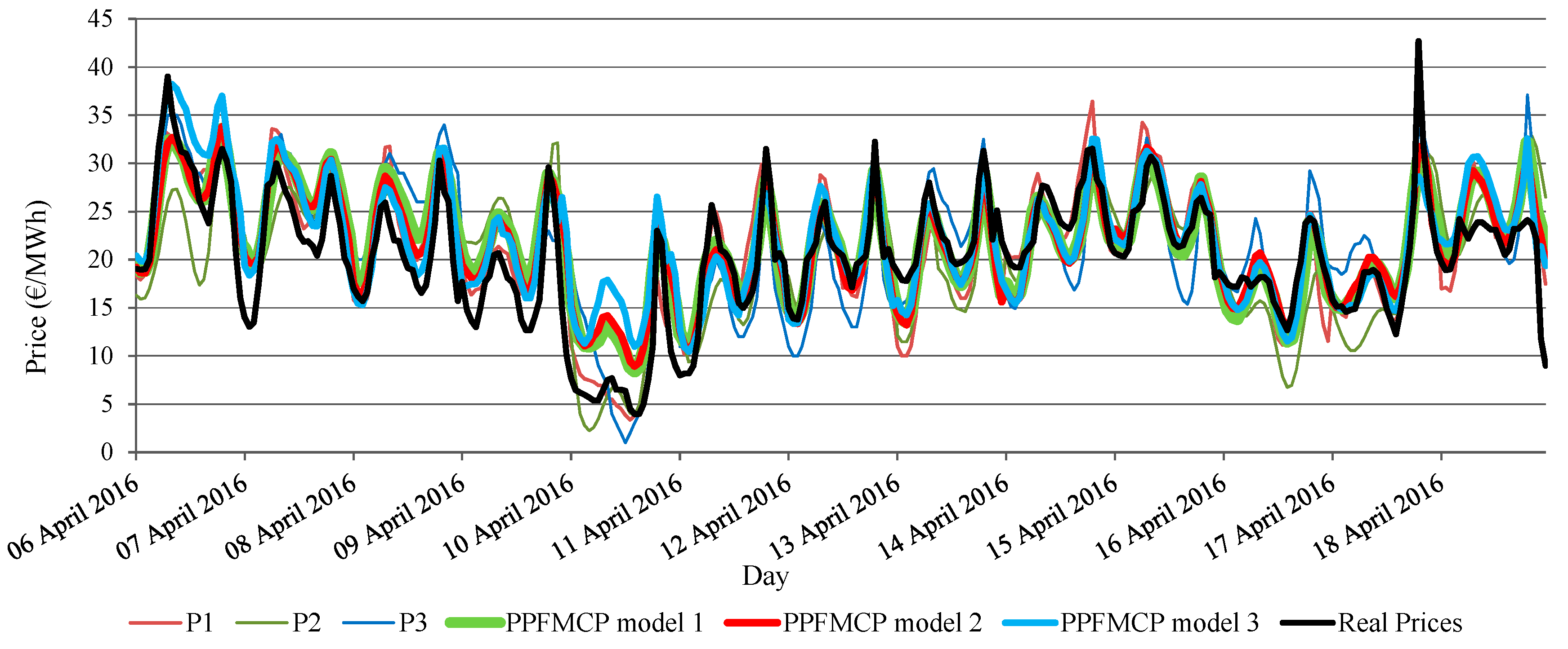
The point (spot) forecasts (expected values of the hourly price) of PPFMCP models 1, 2 and 3 are the values, in €/MWh, computed by expression (12). Figure 10 presents point forecasts of PPFMCP models 1, 2 and 3; the (point) forecasts of the three best predictors P1, P2 and P3; and the real hourly price. The point forecasts of PPFMCP models 1 and 2 are fairly similar; the point forecast of PPFMCP model 3 seems to be a bit more different, but close to the point forecasts of PPFMCP models 1 and 2.

Table 6. Mean absolute error values of point forecasts of PPFMCP models and of the three best predictors P1, P2 and P3.

Date	P1	P2	P3	PPFMCP Model 1	PPFMCP Model 2	PPFMCP Model 3
6 April 2016	1.90	2.21	4.56	2.15	2.31	3.66
7 April 2016	2.97	2.76	3.91	3.84	3.72	3.20
8 April 2016	2.62	1.73	3.60	3.92	2.85	2.24
9 April 2016	2.78	3.96	4.17	4.62	4.12	3.89
10 April 2016	2.10	2.94	2.32	5.24	5.69	7.74
11 April 2016	2.87	2.74	3.58	1.99	2.35	2.82
12 April 2016	2.02	2.29	2.28	1.31	1.47	1.74
13 April 2016	4.22	3.22	4.06	2.30	2.36	1.77
14 April 2016	1.87	2.77	2.16	2.41	2.59	2.66
15 April 2016	1.81	2.93	1.97	1.03	1.41	1.23
16 April 2016	2.76	4.00	2.87	1.66	1.20	1.34
17 April 2016	1.53	1.99	2.66	1.81	1.78	1.56
18 April 2016	3.35	2.78	5.49	3.87	3.30	4.19
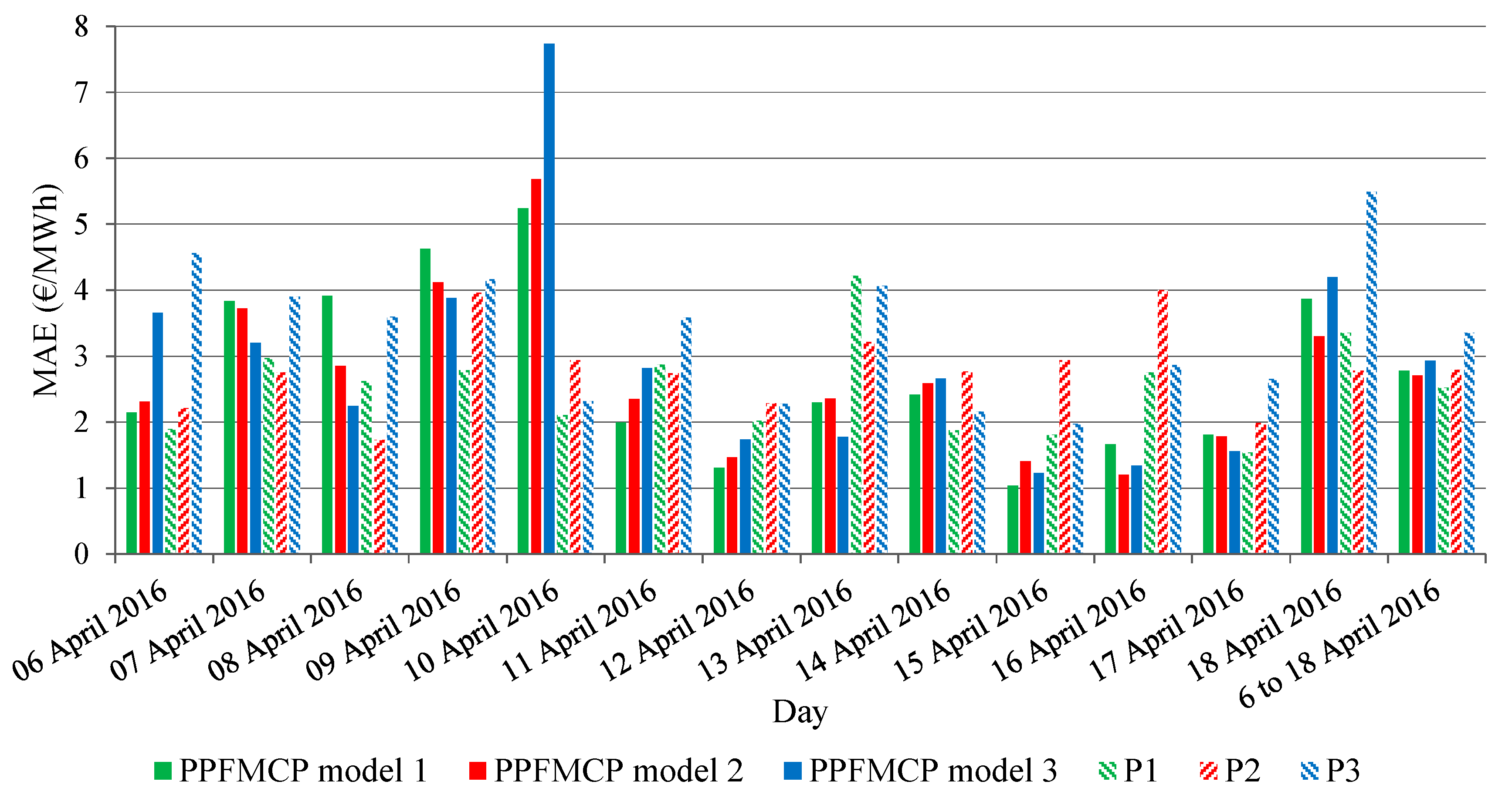
6 to 18 April 2016	2.52	2.79	3.36	2.78	2.70	2.93

and Figure 11 give the mean absolute error values (MAE in Table 6 and Figure 11) of the point forecasts of the three probabilistic models and the mean absolute error values of the (point) forecasts of the three best predictors P1, P2 and P3, corresponding to the period from the 6th to 18th of April 2016, and to each day of this period.

As shown in Table 6, PPFMCP model 2 is the model with a better performance (the MAE value is 2.70 €/MWh, for the 6th to 18th of April 2016); PPFMCP model 1 is close to the former model (the MAE value is 2.78 €/MWh); PPFMCP model 3 obtains a worse performance (the MAE value is 2.93 €/MWh). Comparing the performances of PPFMCP models with those of the individual predictors, we conclude that none of the probabilistic models beats predictor P1, but PPFMCP model 2 and PPFMCP model 1 surpass predictor P2, and all three PPFMCP models beat predictor P3 as well as all the remaining predictors. Considering that predictors P1 and P2 have a significant better performance in comparison with other predictors, we consider that the best predictor P1 was expected not to be beaten by PPFMCP models. It is necessary to remember that predictors P1 and P2 are used by experienced professional price forecasters with access to non-public data.

Figure 11 shows that, for the first week of the competition, PPFMCP models perform often worse than individual predictor P1; but the performance of probabilistic models is usually better during the second week than the performance in the first week. This fact can be explained because most of the predictors improved their performance progressively during the competition (with less dispersion among their spot forecasts); thus, forecasts of PPFMCP models resulted in better performances progressively.

The Loss function Indicator (LI) calculated according to Equation (15) in €/MWh, and the Reliability Indicator (RI) calculated according to Equation (17) in %, were used to evaluate the uncertainty associated with the probabilistic price forecasts of PPFMCP models.

Table 7. Values of indicators LI and RI.

Indicator	PPFMCP Model 1	PPFMCP Model 2	PPFMCP Model 3
LI (€/MWh)	22.1	21.7	26.3
RI (%)	54	57	43

shows the values of indicators LI and RI for the three PPFMCP models. From the point of view of representing the non-explainable information of the forecasts of PPFMCP models, the values of indicator LI and the values of the indicator RI, in Table 7, are consistent when comparing PPFMCP models. PPFMCP model 2, which utilizes aggregation of price forecasts of the predictors by means of weight values according to a daily rank of the predictors, is the best probabilistic model. The second best model is PPFMCP model 1, which uses aggregation by the averaging of price forecasts of the predictors. The last preferred model is PPFMCP model 3, which uses aggregation by means of optimized weights. This performance order of the PPFMCP models is consistent with the order obtained by the mean absolute errors analysis from Table 6.

The Loss function Indicator values for each quantile, LI_p, are represented in Figure 12. The number of quantiles, $nq$, was 9, corresponding to probabilities between 0.1 and 0.9 ($p$ = 0.1, 0.2, 0.3, …. 0.9). An ideal bell shape of $L{I}_p$ should show “central” quantiles with relatively higher values of $L{I}_p$. Ideally the bell shape should be symmetrical, “centred” in quantile Q50 (which represents a probability of 0.5). Figure 12 shows that PPFMCP models 1 and 2 are quite similar, being PPFMCP model 2 slightly better. Both are clearly better than PPFMCP model 3 from the point of view of LI_p.

Figure 13 shows the reliability diagrams for PPFMCP models. The number of probability intervals, $npi$, is 10; probability intervals range from probability interval 0–0.1 to interval 0.9–1. It is important to observe that all intervals have the same length (length of value 0.1). In Figure 13, the target frequency is 10% for each probability interval, except for those with the indication “<min” or “>max” which have a null value for the target frequency. The observed frequencies, (100 × fobs_pi), as a percentage, are situated in indication “˂min” of Figure 13 with notable values, as well as in some of the probability intervals with lower probability values. This fact occurs because most of the predictors generally provided forecasts with bias in excess in the competition, being this more frequent during the first week of the competition period. The observed frequencies of PPFMCP models 1 and 2 for near “central” probability intervals seem to form some parts of bell shapes roughly, which indicates that the PDFs of these probabilistic models are not sharpened enough, probably due to the influence of the predictors with worse performances. From this point of view (sharpened shape of PDFs), PPFMCP model 2 can be a bit better with respect to PPFMCP model 1.

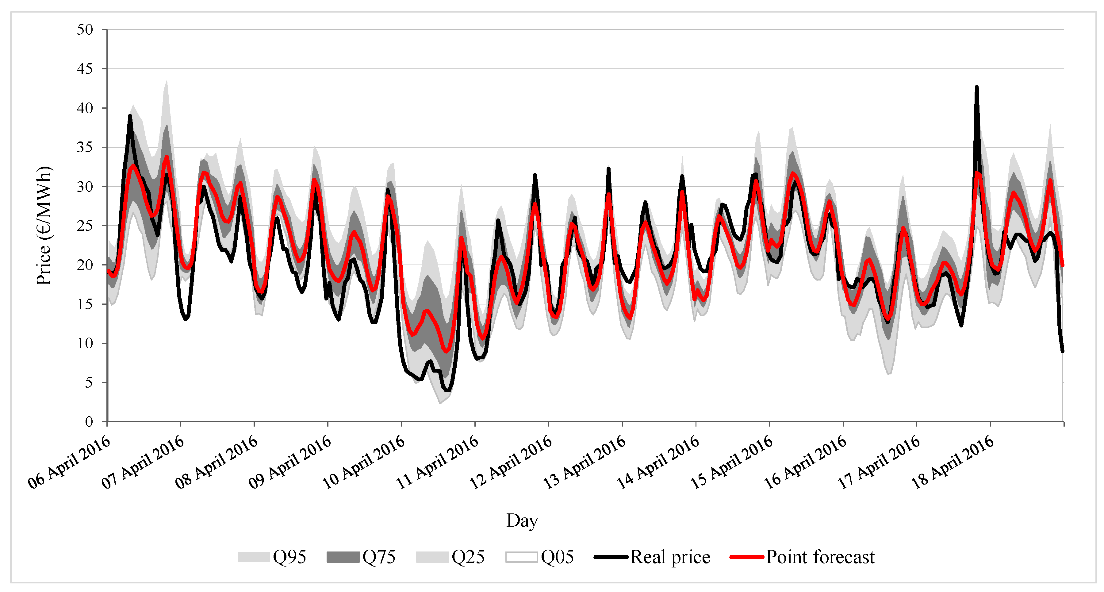
Lastly, Figure 14 shows the probabilistic forecasts provided by PPFMCP model 2 in the last 13 days of the competition period. Observe that only the forecasts for those 13 days were available because the first day of the competition period was needed to provide the first rank used to obtain the weights for PPFMCP model 2. In Figure 14 are represented the quantiles corresponding to probability values of 0.05, 0.25, 0.75 and 0.95, as well as the point forecast provided by PPFMCP model 2 (the expected value obtained with Equation (8)), and the real price.

5. Conclusions

This article presents original probabilistic price forecasting models (PPFMCP models), by aggregation of competitive predictors for the day-ahead hourly probabilistic price forecasting. PPFMCP models were applied to the real-life case of the MIBEL.

The EEM2016 electricity price forecast competition (EEM2016 EPF competition), a real-time price forecast competition on the COMPLATT (competition platform) that corresponded to an active and realistic framework analogous to real-world situations, was first time launched in April 2016, where a total of forty four predictors provided point (spot) price forecasts for the MIBEL on a daily rolling basis. Predictors were point price forecasting tools used by participants in the EEM2016 EPF competition. Historical hourly data, corresponding to the year 2015, were provided to the competition participants. During the competition period, a daily update of data (rolling data) was provided. The data available for the predictors were hourly prices on previous days, regional-aggregated hourly power demands and hourly power generations of most of the types of electricity production on the previous day, hourly power demands in the previous week, forecasts of hourly demand and wind power generation for the Spanish area, weather forecasts (hourly wind speed, wind direction, precipitation, temperature and irradiation) for the day-ahead in the region (mainland of Portugal and Spain), and chronological data. The predictors were globally ranked, according to mean absolute errors for the competition period, which led to the selection of the twenty best predictors (predictors P1 to P20).

The novel PPFMCP models are based on the aggregation of the best predictors (P1 to P20). For each hour, the point price forecasts of the predictors constitute an ensemble that is used to obtain the parameter values of the PDF of a Beta distribution for the output variable (hourly price). PDFs are obtained directly from the expected and variance values associated with such ensemble using three aggregation strategies of price forecasts of the predictors, which correspond to three probabilistic price forecasting models. PPFMCP model 1 uses aggregation by the averaging of price forecasts of the predictors; PPFMCP model 2 uses aggregation of price forecasts of the predictors by means of weight values according to a daily rank of the predictors; and aggregation by means of optimized weights is applied in PPFMCP model 3.

Thus, valuable quantitative probabilistic information of the behaviour of the hourly price variable can be determined from the PDF for each hour of the probabilistic price forecast of each PPFMCP model, which allows the evaluation of risk decisions based on the price to be made, as well as the calculation on the probability to have prices which are higher than some price limits, the calculation on the probability to obtain prices in a target interval, and the calculation of quantiles.

PPFMCP models were satisfactorily applied to the real-life case study of the MIBEL. Results of the PPFMCP models are described in this article, including PDFs of Beta distributions for probabilistic forecasts, as well as daily weight values of these probabilistic models.

Two appropriate indicators, called Reliability Indicator (RI) and Loss function Indicator (LI), are also introduced, which allow the uncertainty associated to probabilistic price forecasts of the PPFMCP models to be evaluated.

Results from PPFMCP models, showed that PPFMCP model 2 was the best probabilistic model from the point of view of the mean absolute error values, as well as from the point of view of LI and RI values; and results also showed that PPFMCP model 1 was the second best probabilistic model.

The probabilistic price forecasting models of this article and the pragmatic calculations applied to the PDFs associated with their day-ahead probabilistic price forecasts can be useful for business agents of electrical energy markets and other players who act in the electric power industry.

References

- Weron, R. Electricity price forecasting: A review of the state-of-the-art with a look into the future. Int. J. Forecast. 2014, 30, 1030–1081. [Google Scholar] [CrossRef]
- Murthy, G.G.P.; Sedidi, V.; Panda, A.K.; Rath, B.N. Forecasting electricity prices in deregulated wholesale spot electricity market: A review. Int. J. Energy Econ. Policy 2014, 4, 32–42. [Google Scholar]
- Nogales, F.J.; Contreras, J.; Conejo, A.J.; Espínola, R. Forecasting Next-Day Electricity Prices by Times Series Models. IEEE Trans. Power Syst. 2002, 17, 342–348. [Google Scholar] [CrossRef]
- Conejo, A.J.; Contreras, J.; Espínola, R.; Plazas, M.A. Forecasting electricity prices for a day-ahead pool-based electric energy market. Int. J. Forecast. 2005, 21, 435–462. [Google Scholar] [CrossRef]
- Cruz, A.; Muñoz, A.; Zamora, J.L.; Espínola, R. The effect of wind generation and weekday on Spanish electricity spot price forecasting. Electr. Power Syst. Res. 2011, 81, 1924–1935. [Google Scholar] [CrossRef]
- Zareipour, H.; Cañizares, C.A.; Bhattacharya, K.; Thomson, J. Application of public-domain market information to forecast Ontario’s wholesale electricity prices. IEEE Trans. Power Syst. 2006, 21, 1707–1717. [Google Scholar] [CrossRef]
- Weron, R.; Misiorek, A. Forecasting spot electricity prices: A comparison of parametric and semiparametric time series models. Int. J. Forecast. 2008, 24, 744–763. [Google Scholar] [CrossRef] [Green Version]
- Tan, Z.; Zhang, J.; Wang, J.; Xu, J. Day-ahead electricity price forecasting using wavelet transform combined with ARIMA and GARCH models. Appl. Energy 2010, 87, 3606–3610. [Google Scholar] [CrossRef]
- Bordignon, S.; Bunn, D.W.; Lisi, F.; Nan, F. Combining day-ahead forecasts for British electricity prices. Energy Econ. 2013, 35, 88–103. [Google Scholar] [CrossRef]
- Ziel, F. Forecasting Electricity Spot Prices Using Lasso: On Capturing the Autoregressive Intraday Structure. IEEE Trans. Power Syst. 2016, 31, 4977–4987. [Google Scholar] [CrossRef]
- Huurman, C.; Ravazzolo, F.; Zhou, C. The power of weather. Comput. Stat. Data Anal. 2012, 56, 3793–3807. [Google Scholar] [CrossRef]
- Guo, J.J.; Luh, P.B. Improving market clearing price prediction by using a committee machine of neural networks. IEEE Trans. Power Syst. 2004, 19, 1867–1876. [Google Scholar] [CrossRef]
- Lin, W.-M.; Gow, H.-J.; Tsai, M.-T. Electricity price forecasting using Enhanced Probability Neural Network. Energy Convers. Manag. 2010, 51, 2707–2714. [Google Scholar] [CrossRef]
- Singhal, D.; Swarup, K.S. Electricity price forecasting using artificial neural networks. Int. J. Electr. Power Energy Syst. 2011, 33, 550–555. [Google Scholar] [CrossRef]
- Monteiro, C.; Fernandez-Jimenez, L.; Ramirez-Rosado, I. Explanatory Information Analysis for Day-Ahead Price Forecasting in the Iberian Electricity Market. Energies 2015, 8, 10464–10486. [Google Scholar] [CrossRef]
- Papadimitriou, T.; Gogas, P.; Stathakis, E. Forecasting energy markets using support vector machines. Energy Econ. 2014, 44, 135–142. [Google Scholar] [CrossRef]
- Alamaniotis, M.; Bargiotas, D.; Bourbakis, N.G.; Tsoukalas, L.H. Genetic Optimal Regression of Relevance Vector Machines for Electricity Pricing Signal Forecasting in Smart Grids. IEEE Trans. Smart Grid 2015, 6, 2997–3005. [Google Scholar] [CrossRef]
- Ghasemi, A.; Shayeghi, H.; Moradzadeh, M.; Nooshyar, M. A novel hybrid algorithm for electricity price and load forecasting in smart grids with demand-side management. Appl. Energy 2016, 177, 40–59. [Google Scholar] [CrossRef]
- Rodriguez, C.P.; Anders, G.J. Energy Price Forecasting in the Ontario Competitive Power System Market. IEEE Trans. Power Syst. 2004, 19, 366–374. [Google Scholar] [CrossRef]
- Amjady, N. Day-Ahead Price Forecasting of Electricity Markets by a New Fuzzy Neural Network. IEEE Trans. Power Syst. 2006, 21, 887–896. [Google Scholar] [CrossRef]
- Li, G.; Liu, C.-C.; Mattson, C.; Lawarree, J. Day-Ahead Electricity Price Forecasting in a Grid Environment. IEEE Trans. Power Syst. 2007, 22, 266–274. [Google Scholar] [CrossRef]
- Saini, L.M.; Aggarwal, S.K.; Kumar, A. Parameter optimisation using genetic algorithm for support vector machine-based price-forecasting model in National electricity market. IET Gener. Transm. Distrib. 2010, 4, 36. [Google Scholar] [CrossRef]
- Catalão, J.P.S.; Pousinho, H.M.I.; Mendes, V.M.F. Hybrid wavelet-PSO-ANFIS approach for short-term electricity prices forecasting. IEEE Trans. Power Syst. 2011, 26, 137–144. [Google Scholar] [CrossRef]
- Mandal, P.; Haque, A.U.; Meng, J.; Srivastava, A.K.; Martinez, R. A novel hybrid approach using wavelet, firefly algorithm, and fuzzy ARTMAP for day-ahead electricity price forecasting. IEEE Trans. Power Syst. 2013, 28, 1041–1051. [Google Scholar] [CrossRef]
- Filho, J.C.R.; Affonso, C.D.M.; De Oliveira, R.C.L. Energy price prediction multi-step ahead using hybrid model in the Brazilian market. Electr. Power Syst. Res. 2014, 117, 115–122. [Google Scholar] [CrossRef]
- Osório, G.J.; Matias, J.C.O.; Catalão, J.P.S. Electricity prices forecasting by a hybrid evolutionary-adaptive methodology. Energy Convers. Manag. 2014, 80, 363–373. [Google Scholar] [CrossRef]
- Singh, N.; Mohanty, S.R.; Dev Shukla, R. Short term electricity price forecast based on environmentally adapted generalized neuron. Energy 2017, 125, 127–139. [Google Scholar] [CrossRef]
- Bento, P.M.R.; Pombo, J.A.N.; Calado, M.R.A.; Mariano, S.J.P.S. A bat optimized neural network and wavelet transform approach for short-term price forecasting. Appl. Energy 2018, 210, 88–97. [Google Scholar] [CrossRef]
- Hong, T.; Fan, S. Probabilistic electric load forecasting: A tutorial review. Int. J. Forecast. 2016, 32, 914–938. [Google Scholar] [CrossRef]
- Nowotarski, J.; Weron, R. Recent advances in electricity price forecasting: A review of probabilistic forecasting. Renew. Sustain. Energy Rev. 2018, 81, 1548–1568. [Google Scholar] [CrossRef]
- Amjady, N.; Hemmati, M. Energy price forecasting - problems and proposals for such predictions. IEEE Power Energy Mag. 2006, 4, 20–29. [Google Scholar] [CrossRef]
- Misiorek, A.; Trueck, S.; Weron, R. Point and Interval Forecasting of Spot Electricity Prices: Linear vs. Non-Linear Time Series Models. Stud. Nonlinear Dyn. Econom. 2006, 10. [Google Scholar] [CrossRef] [Green Version]
- Dudek, G. Multilayer perceptron for GEFCom2014 probabilistic electricity price forecasting. Int. J. Forecast. 2016, 32, 1057–1060. [Google Scholar] [CrossRef]
- Panagiotelis, A.; Smith, M. Bayesian density forecasting of intraday electricity prices using multivariate skew t distributions. Int. J. Forecast. 2008, 24, 710–727. [Google Scholar] [CrossRef]
- Efron, B.; Tibshirani, R.J. An introduction to the Bootstrap; Chapman & Halll: Boca Raton, FL, USA, 1993. [Google Scholar]
- Alonso, A.M.; García-Martos, C.; Rodríguez, J.; Jesús Sánchez, M. Seasonal Dynamic Factor Analysis and Bootstrap Inference: Application to Electricity Market Forecasting. Technometrics 2011, 53, 137–151. [Google Scholar] [CrossRef] [Green Version]
- Rafiei, M.; Niknam, T.; Khooban, M.H. Probabilistic electricity price forecasting by improved clonal selection algorithm and wavelet preprocessing. Neural Comput. Appl. 2017, 28, 3889–3901. [Google Scholar] [CrossRef]
- Nowotarski, J.; Weron, R. Computing electricity spot price prediction intervals using quantile regression and forecast averaging. Comput. Stat. 2015, 30, 791–803. [Google Scholar] [CrossRef]
- Gaillard, P.; Goude, Y.; Nedellec, R. Additive models and robust aggregation for GEFCom2014 probabilistic electric load and electricity price forecasting. Int. J. Forecast. 2016, 32, 1038–1050. [Google Scholar] [CrossRef]
- Maciejowska, K.; Nowotarski, J. A hybrid model for GEFCom2014 probabilistic electricity price forecasting. Int. J. Forecast. 2016, 32, 1051–1056. [Google Scholar] [CrossRef]
- Tahmasebifar, R.; Sheikh-El-Eslami, M.K.; Kheirollahi, R. Point and interval forecasting of real-time and day-ahead electricity prices by a novel hybrid approach. IET Gener. Transm. Distrib. 2017, 11, 2173–2183. [Google Scholar] [CrossRef]
- Rafiei, M.; Niknam, T.; Khooban, M.H. Probabilistic Forecasting of Hourly Electricity Price by Generalization of ELM for Usage in Improved Wavelet Neural Network. IEEE Trans. Ind. Inform. 2017, 13, 71–79. [Google Scholar] [CrossRef]
- Andrade, J.R.; Filipe, J.; Reis, M.; Bessa, R.J. Probabilistic price forecasting for day-ahead and intraday markets: Beyond the statistical model. Sustainability 2017, 9. [Google Scholar] [CrossRef]
- Market Operator of the Iberian Electricity Market, OMIE. Available online: http://www.omie.es (accessed on 7 March 2018).
- The Iberian Energy Derivatives Exchange, OMIP. Available online: http://www.omip.pt (accessed on 7 March 2018).
- Price Forecast Competition. In Proceedings of the 13th International Conference on the European Energy Market, Porto, Portugal, 6–9 June 2016; Available online: http://www.eem2016.com/price-forecast-competition/COMPLATT_MKT_V4.pdf (accessed on 16 February 2018).
- Ramanathan, R.; Engle, R.; Granger, C.W.J.; Vahid-Araghi, F.; Brace, C. Short-run forecasts of electricity loads and peaks. Int. J. Forecast. 1997, 13, 161–174. [Google Scholar] [CrossRef]
- EUNITE Peak Load Forecast Competition. Available online: http://www.eunite.org/knowledge/Competitions/1st_competition/1st_competition.htm. (accessed on 7 March 2018).
- Hong, T.; Pinson, P.; Fan, S. Global energy forecasting competition 2012. Int. J. Forecast. 2014, 30, 357–363. [Google Scholar] [CrossRef]
- McGovern, A.; Gagne, D.J.; Basara, J.; Hamill, T.M.; Margolin, D. Solar energy prediction: An international contest to initiate interdisciplinary research on compelling meteorological problems. Bull. Am. Meteorol. Soc. 2015, 96, 1388–1393. [Google Scholar] [CrossRef]
- Hong, T.; Pinson, P.; Fan, S.; Zareipour, H.; Troccoli, A.; Hyndman, R.J. Probabilistic energy forecasting: Global Energy Forecasting Competition 2014 and beyond. Int. J. Forecast. 2016, 32, 896–913. [Google Scholar] [CrossRef] [Green Version]
- Institute for Systems and Computer Engineering, Technology and Science (INESC TEC). Available online: https://www.inesctec.pt/ (accessed on 7 March 2018).
- Red Eléctrica de España (REE). Spanish Transmission System Operator. Available online: http://www.ree.es/es/actividades/demanda-y-produccion-en-tiempo-real (accessed on 7 March 2018).
- Redes Energéticas Nacionais (REN). Portuguese Transmission System Operator. Available online: http://www.centrodeinformacao.ren.pt/EN/Pages/CIHomePage.aspx (accessed on 7 March 2018).
- Nadarajah, S.; Gupta, A.K. Generalizations and related univariate distributions. In Handbook of Beta Distribution and Its Applications; Gupta, A.K., Nadarajah, S., Eds.; Marcel Dekker Inc.: New York, NY, USA, 2004; pp. 97–163. ISBN 0-8247-5396-8. [Google Scholar]
Figure 1.
Monthly electricity generation, demand and real price of electricity in 2015.
Figure 2.
Monthly electricity generation, demand and real price of electricity in 2016.
Figure 3.
Hourly mean electricity generation, demand and real price of electricity in April 2015.
Figure 4.
Hourly mean electricity generation, demand and real price of electricity in April 2016.
Figure 5.
Forecasts provided by the twenty best predictors and hourly real prices.
Figure 6.
Histogram of daily mean errors for the day-ahead forecast (D + 1) of prices for the two weeks of the competition.
Figure 7.
Values of MAE(D + 1) and MAPE(D + 1) for each day of the competition period and values of MAE for “all days” of the competition period, MAEg(D + 1), for the best nine predictors.
Figure 8.
Values of MAEg(D + 1) to MAEg(D + 5), and MAPEg(D + 1) to MAPEg(D + 5), for predictors P1 to P9.
Figure 9.
Probability density functions (PDFs) of the PPFMCP models for hours 11 h, 12 h, and 13 h on the 14th of April, 2016. (a) PPFMCP model 1; (b) PPFMCP model 2; (c) PPFMCP model 3.
Figure 10.
Point forecasts for the three best predictors P1, P2 and P3; point forecasts of PPFMCP models 1, 2 and 3; and real prices.
Figure 11.
Mean absolute error values of point forecast of PPFMCP models and of the three best predictors.
Figure 12.
Loss function Indicator for each quantile.
Figure 13.
Reliability diagrams for PPFMCP models.
Figure 14.
Probabilistic forecasts provided by PPFMCP model 2.