Arrays of Point-Absorbing Wave Energy Converters in Short-Crested Irregular Waves

Abstract

For most wave energy technology concepts, large-scale electricity production and cost-efficiency require that the devices are installed together in parks. The hydrodynamical interactions between the devices will affect the total performance of the park, and the optimization of the park layout and other park design parameters is a topic of active research. Most studies have considered wave energy parks in long-crested, unidirectional waves. However, real ocean waves can be short-crested, with waves propagating simultaneously in several directions, and some studies have indicated that the wave energy park performance might change in short-crested waves. Here, theory for short-crested waves is integrated in an analytical multiple scattering method, and used to evaluate wave energy park performance in irregular, short-crested waves with different number of wave directions and directional spreading parameters. The results show that the energy absorption is comparable to the situation in long-crested waves, but that the power fluctuations are significantly lower.

1. Introduction

Ocean waves provide a clean, renewable energy source with a large potential to contribute to the energy demand without negative environmental or climate impact. There is a large number of different technology approaches for conversion of wave energy to electricity, and very few have reached a commercial maturity. Common for many of the technologies is that a large-scale electricity production requires that many wave energy converters (WECs) are deployed together in arrays, or parks. In particular, this is true for the point-absorber concept considered in this study.

Since the devices in the park will interact hydrodynamically by scattered and radiated waves spreading throughout the park, it is of importance to determine the optimal park layout that achieves maximum electricity production with minimum power fluctuations and costs. Since the early works on wave energy, studying and optimizing wave energy array layouts have been main topics of interest [1,2,3], and remains an active area of research today [4,5,6,7,8,9].

Many parameters affect the performance of the park. The impact of increasing the number of devices in a park on both the energy absorption and power fluctuations was investigated in [10,11,12,13,14], and it was seen that increasing the number of WECs by around 30% may reduce the power fluctuations by roughly 7% and the average power of each device by 3% [14], and, in experiments, it was seen that, in an array with 24 WECs, up to 26% of the energy yield from an equivalent number of isolated WECs may be lost due to interference effects [13]. The effect of the individual device dimensions was studied in [14,15,16], and it was seen that the total performance of the park may increase if WECs of different dimensions are deployed together. The separation distance between devices and the layout of the park has been studied in a large number of works [11,13,17,18,19,20,21], and separation distances ranging from $4R$, where R is the radius of the float, up to a few hundred metres, have been established, above which the interaction effects between devices can be neglected. Obviously, the wave climate, the incident wave directions and the bathymetry are other factors that may affect the performance of the park, which has been studied in [14,22,23], among others. Most of the work has been based on numerical or analytical modelling, but a few examples of experimental studies exist, both in wave tank [13,24] and offshore [12].

Much of the mentioned works on optimal configurations of wave energy parks have considered only incident regular waves, and even if irregular waves have been considered, almost all have considered only long-crested, unidirectional waves. However, real ocean waves can be multidirectional, or short-crested, with irregular waves travelling in different directions simultaneously, and this is likely to affect the performance of the wave energy parks. An array of 12 oscillating wave surge converters was studied in short-crested waves in [7] and it was found that the average absorbed energy of the park was slightly lower than when it was operating in unidirectional waves. A similar conclusion was found in [25] for attenuator type WECs, and it was also found that the relative pitch motions were reduced in short-crested waves. Wave run-up on bottom-mounted cylinders was found to increase in short-crested waves studied with semi-analytical methods in [26], and the presence of near-trapped modes was reduced. The wake effect behind WEC arrays was studied in [17,27], and both papers found that the wake was reduced when directional wave spreading was taken into account. This effect and other wave energy array effects in short-crested waves was also investigated experimentally in [24].

From the abovementioned studies, it is clear that the performance of wave energy parks might change when operating in short-crested waves as opposed to in unidirectional, long-crested waves. In [28], a semi-analytical model for computing the hydrodynamical forces and interactions in a wave energy park of point-absorbing WECs was presented, based on the approximate method in [21]. An interaction distance cut-off was introduced, which enabled accurate and fast modelling of large parks with over 100 devices. The method was extended to enable point-absorber devices of different individual dimensions in [16], and has been coupled with a genetic algorithm for multiple parameter optimization of wave energy parks in [29]. The approach provides a fast and reliable method to assess and optimize all involved parameters in a park, including park layout and individual WEC dimensions. In the present paper, the method is extended to also describe short-crested waves, and used to study the performance of wave energy parks in more realistic seas.

The paper is organized as follows. The theory of multiple scattering with short-crested waves is described in Section 2.1 and Section 2.2, with the notation and equations of motion for wave energy parks established in Section 2.1 and the multiple scattering method in Section 2.2. The resulting method is used to study short-crested waves and wave energy park performance and discussed in Section 3.1, Section 3.2 and Section 3.3. Conclusions from the study are presented in Section 4.

2. Method

2.1. Wave Energy Park Model

Consider an array of N point-absorbing wave energy converters, each consisting of a surface buoy with radius $R^i$ and draft $d^i$ connected to a linear generator at the seabed. The generator consists of a translator moving vertically within a stator, and is characterized by a generator damping ${\mathsf{\Gamma }}^i$. The WEC model is based on the wave energy technology developed at Uppsala University, Sweden. The approach for the wave energy concept is based on simplicity to improve the life-expectancy of the device and reduce capital and maintenance costs—the generator consists of as few moving parts as possible, and is situated at the seabed to be protected from storms or other extreme wave conditions. By changing the buoy and generator dimensions, as well as the connection line length, the WEC can be adapted to different wave climates and deployment site conditions. Simulated and experimentally measured performance in different wave conditions was presented for earlier prototypes of the device in [30,31], and more information about the device can be found in [10,12].

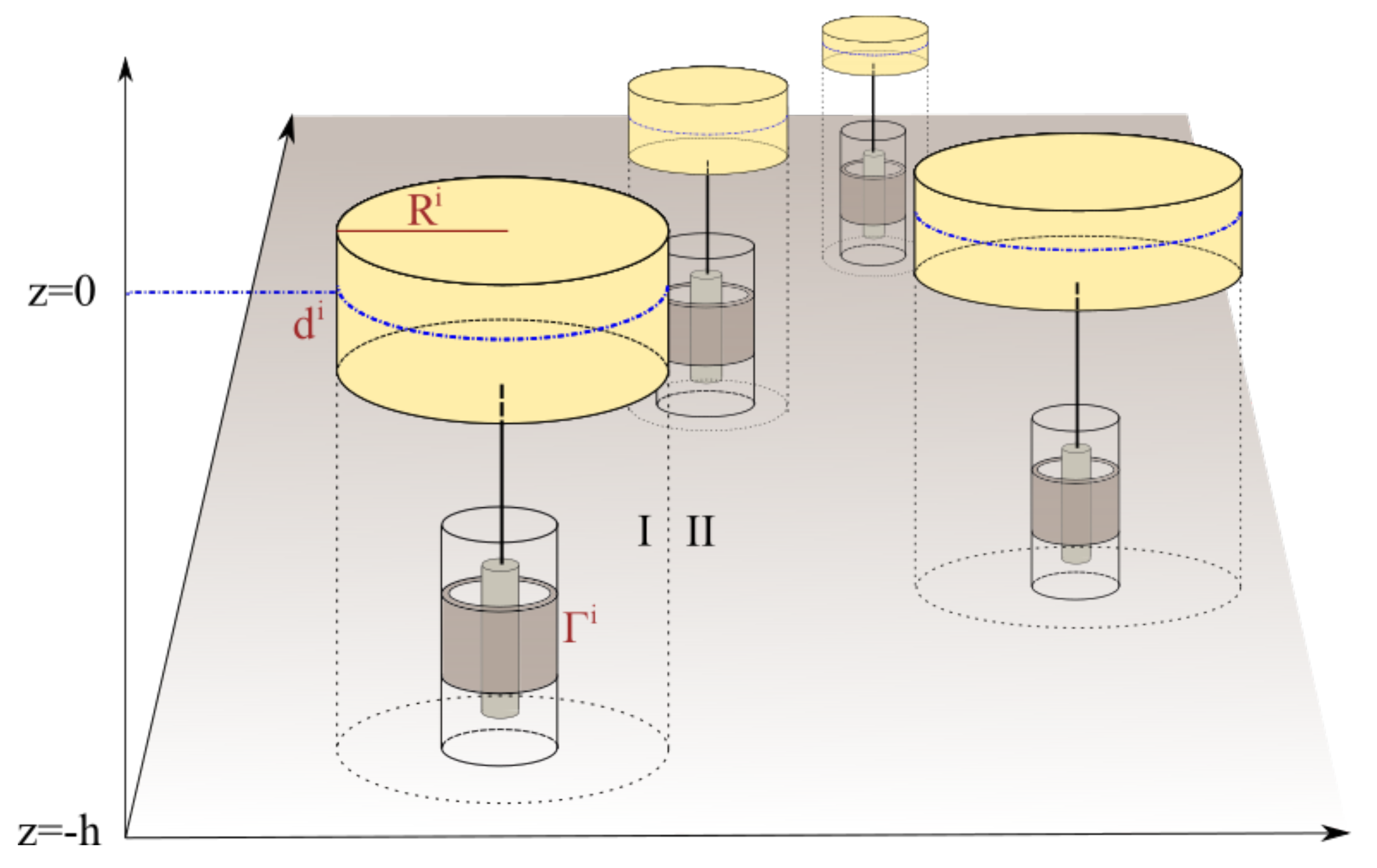
The water depth is h and the density of the water is $\rho$. The coordinate system is chosen such that $z=0$ at the still water surface and $z=-h$ at the seabed. Local cylindrical coordinate systems $(r,\theta ,z)$ are defined at the origin $(x^i,y^i,z)$ of each buoy. An illustration of the wave energy park is shown in Figure 1.

The motion of the buoys and the translator are given by the coupled equations of motion

$$\begin{array}{cc}\hfill m_b^i{\ddot{\overline{x}}}_b^i\left(t\right)& =-{\int \int }_{S^i}p\left(t\right)\overline{n}dS-{\overline{F}}_{\mathrm{line}}^i\left(t\right)-m_b^{i}g\widehat{z},\hfill \end{array}$$

(1)

$$\begin{array}{cc}\hfill m_t^i{\ddot{z}}_t^i\left(t\right)& ={\overline{F}}_{\mathrm{line}}^i\left(t\right)+{\overline{F}}_{\mathrm{PTO}}^i\left(t\right)-m_t^{i}g\widehat{z},\hfill \end{array}$$

(2)

where $m_b^i$ and $m_t^i$ are the mass of the buoy and translator, respectively, p contains both the dynamical and hydrostatical pressure, ${\overline{F}}_{\mathrm{line}}^i$ is the line in the force connecting the buoy and the translator, and ${\overline{F}}_{\mathrm{PTO}}^i$ is the damping force of the generator. The normal vector $\overline{n}$ is defined to point away from the body surface, into the fluid. The hydrodynamical forces will be solved using linear potential flow theory, described in more detail in Section 2.2.1. Under the constraints that the connection between the buoy and translator is stiff, and that the buoy is moving in heave only, a single equation of motion describes the dynamics of the system

$$m^i{\ddot{z}}^i\left(t\right)=F_{\mathrm{exc}}^i\left(t\right)+F_{\mathrm{rad}}^i\left(t\right)+F_{\mathrm{stat}}^i\left(t\right)+F_{\mathrm{PTO}}^i\left(t\right),$$

(3)

where $m^i=m_b^i+m_t^i$ is the total masses of the buoy and the translator, $F_{\mathrm{exc}}^i$ is the excitation force due to the incident and scattered waves, $F_{\mathrm{rad}}^i$ the radiation force due to the oscillations of the buoy, $F_{\mathrm{stat}}^i=-\rho g\pi R^i{z}^i$ the hydrostatic restoring force and $F_{\mathrm{PTO}}^i=-{\mathsf{\Gamma }}^i{\dot{z}}^i\left(t\right)$ the power take-off damping of the generator.

The hydrodynamical forces will be computed in the frequency domain, where the equivalent equation of motion (3) reads

$${\left[-{\omega }^2(m+m_{\mathrm{add}})-i\omega (\mathsf{\Gamma }+B)+\rho g\pi R\right]}_j^i{z}^j\left(\omega \right)=F_{\mathrm{exc}}^i\left(\omega \right),$$

(4)

where the radiation force was divided into an added mass term proportional to the acceleration and a radiation damping term proportional to the velocity, $F_{\mathrm{rad}}^i\left(\omega \right)={[-i\omega m_{\mathrm{add}}+B]}_j^{i}i\omega z^j\left(\omega \right)$ and the excitation force can be divided into an excitation force coefficient vector and the incident waves, $F_{\mathrm{exc}}^i\left(\omega \right)=f_{\mathrm{exc}}^i\left(\omega \right)A^i\left(\omega \right)$. The incident waves will be irregular, short-crested waves, described in more detail in Section 2.2.2.

When the equations of motion have been solved in the frequency domain, the result is obtained in the time domain by the inverse Fourier transform, and the absorbed power of each WEC at each point in time is computed as

$$P^i\left(t\right)={\mathsf{\Gamma }}^i{\left[\dot{z}\left(t\right)\right]}^2,$$

(5)

and the total power of the park is the sum of the absorbed power of all devices in the park. The absorbed power will vary over time with the incident waves, and the resulting total power of the park will display power fluctuations. To connect the power from a park to the electrical grid, low power fluctuations are required. Large power peaks will require over-dimensional, expensive power electronics system, and instants with no power will create unwanted power outages. The power fluctuations can be quantified by the normalized variance, defined in terms of the standard deviation $\sigma$ as

$$v=\frac{{\sigma }^2\left(P_{\mathrm{tot}}\left(t\right)\right)}{{\overline{P}}_{\mathrm{tot}}}.$$

(6)

A common way to represent the interaction in a park is with the interaction factor, or q-factor [1], defined as the ratio between the time averaged power absorbed by the park, and the sum of all devices’ individual power absorption if they were isolated,

$$q=\frac{{\overline{P}}_{\mathrm{tot}}}{{\sum }_{i=1}^N{\overline{P}}_{\mathrm{isolated}}^i}.$$

(7)

An individual q-factor for each WEC in the park can also be defined as the ratio between its averaged absorbed power and the average it would absorb in isolation,

$$q^i=\frac{{\overline{P}}^i}{{\overline{P}}_{\mathrm{isolated}}^i}.$$

(8)

Although cases can be found where the interaction factor is larger than one, in realistic cases, the interaction effects will be destructive with $q<1$, and optimization of the park interactions will aim to minimize destructive interactions and achieve an interaction factor as close to 1 as possible [3,22]. To allow for direct comparisons, in this paper, the individual q-factor is computed with the same isolated power absorption, i.e., the denominator ${\overline{P}}_{\mathrm{isolated}}^i$ in Equation (8) is computed with the same irregular waves and corresponds to an isolated WEC situated at the origin $(x,y)=(0,0)$. To avoid confusion, the computed values in Equations (7) and (8) will therefore be denoted normalized energy absorption.

2.2. Multiple Scattering Theory with Short-Crested Waves

2.2.1. Linear Potential Flow Theory

Consider a fluid that is incompressible and irrotational, implying that it can be described by potential flow theory using a fluid velocity potential satisfying the Laplace equation, ${\nabla }^2\mathsf{\Phi }=0$, where $\overline{u}=\nabla \mathsf{\Phi }$ is the fluid velocity. Further assume that the viscosity of the fluid can be neglected and that the wave height is small compared to the wave length, so that the boundary constraints at the sea surface can be linearized. The fluid is then described by linear potential flow theory, and the details can be found in many text books such as [32].

The surface elevation of a wave with potential $\mathsf{\Phi }\left(t\right)$ is given by

$$\eta (x,y,t)=-\frac{1}{g}\frac{\partial \mathsf{\Phi }}{\partial t}{|}_{z=0},$$

(9)

where g is the gravitational acceleration constant. The surface elevation in the frequency domain is obtained by Fourier transform,

$$\widehat{\eta }(x,y,\omega )={\int }_{-\infty }^{\infty }\eta (x,y,t)e^{-i\omega t}dt.$$

(10)

Due to the linearity of the problem, the fluid potential can be decomposed into incident, scattered and radiated waves, and from the linear Bernoulli equation the dynamical pressure can be obtained from the fluid potential as $p=-\rho \frac{\partial \mathsf{\Phi }}{\partial t}$, so that the hydrodynamical forces are obtained in the frequency domain as

$$\begin{array}{cc}\hfill {\overline{F}}_{\mathrm{exc}}\left(\omega \right)& =i\omega \rho {\int \int }_S{\varphi }_D\overline{n}dS,\hfill \end{array}$$

(11)

$$\begin{array}{cc}\hfill {\overline{F}}_{\mathrm{rad}}\left(\omega \right)& =i\omega \rho {\int \int }_S{\varphi }_R\overline{n}dS,\hfill \end{array}$$

(12)

where ${\varphi }_D={\varphi }_I+{\varphi }_S$ is the diffraction and ${\varphi }_R$ the radiation potentials and the integration is taken over the wetted surface of the buoy. By solving the multiple scattering problem as described in Section 2.2.3, the fluid potentials can be solved for and the hydrodynamical forces computed according to (11) and (12). With the hydrodynamical forces obtained, the equations of motion in Equation (4) can be solved and the performance of the park evaluated.

2.2.2. Multidirectional Waves

Open ocean waves are assumed, i.e., no reflective structures exist so that there are no phase-locked waves—all the phases are randomly distributed, implying that the wave components are independent of each other. Thus, we can treat the irregular short-crested waves as a superposition of harmonic waves travelling in different directions.

A single harmonic wave travelling in direction $\chi$ away from the x-axis can be described by the surface elevation $\eta (x,y,t)=acos\left(\omega t-\overline{k}·\overline{x}+\phi \right)$, where $\phi$ the phase, and $\omega$ is the angular frequency related to the wave number vector $\overline{k}=(kcos\chi ,ksin\chi ,0)$ by the dispersion relation for ocean waves. When the waves are composed of many waves travelling in independent directions, the surface elevation can be written as the superposition

$$\eta (x,y,t)=\sum _{n=-\infty }^{\infty }\sum _{m=1}^M{a}_{mn}{e}^{i({\omega }_{n}t-{\overline{k}}_{mn}·\overline{x})}=2\sum _{n=0}^{\infty }\sum _{m=1}^M|a_{mn}|cos({\omega }_{n}t-{\overline{k}}_{mn}·\overline{x}+{\phi }_{mn}),$$

(13)

where $a_{mn}$ is hermitian, i.e., $a_{mn}^{*}=a_{m-n}$, the phase is ${\phi }_{mn}=\arg \left(a_{mn}\right)$ and ${\overline{k}}_{mn}·\overline{x}=k_n(xcos{\chi }_m+ysin{\chi }_m)$. The complex amplitude coefficients can be written in terms of the directional wave spectra as

$$2|a_{mn}{|}^2=S({\omega }_n,{\chi }_m)d\omega d\chi ,$$

(14)

where $d\omega ={\omega }_{n+1}-{\omega }_n$ and $d\chi ={\chi }_{m+1}-{\chi }_m$. The expression for the surface elevation turns into an inverse Fourier integral when $d\omega$ becomes infinitesimal and we write $a_{mn}=A({\omega }_n,{\chi }_m)d\omega d\chi$, such that

$$2|A(\omega ,\chi ){|}^{2}d\omega d\chi =S(\omega ,\chi ).$$

(15)

The energy in the waves is given by

$$E=\rho g<{\eta }^2>=\rho g{\int }_0^{\infty }d\omega {\int }_{-\pi }^{\pi }d\chi S(\omega ,\chi ).$$

(16)

The directional wave spectrum can be assumed to be decomposed into a direction independent spectrum and a directional spreading function (DSF)

$$S(\omega ,\chi )=S\left(\omega \right)D(\omega ,\chi ),$$

(17)

where periodicity is required, $D(\omega ,2\pi )=D(\omega ,0)$, and conservation of energy requires that the directional spreading function is normalized

$${\int }_{-\pi }^{\pi }D(\omega ,\chi )d\chi =1.$$

(18)

Several different directional spreading functions have been defined and studied in the literature. A common assumption is that the directional spreading function can be described by a unimodal model parametrized by the mean direction $\overline{\chi }$ and another parameter, such as the spreading parameter or a directional width, so that it is independent of the wave frequency. The default representation, still widely used, was defined in [33] and reads

$$D(\chi -\overline{\chi })=F\left(s\right){cos}^{2s}\left(\frac{\chi -\overline{\chi }}{2}\right),$$

(19)

where $\overline{\chi }$ is the principal wave direction and $F\left(s\right)$ is defined such that the normalization constraint in Equation (18) is satisfied. In [34], the coefficient $F\left(s\right)$ was defined in terms of gamma functions as

$$F\left(s\right)=\frac{2^{2s-1}}{\pi }\frac{{\left(\mathsf{\Gamma }(s+1)\right)}^2}{\mathsf{\Gamma }(2s+1)},$$

(20)

which was later also used in [25], albeit presented differently, for the spreading parameter $s=5,15,25$. Here, we will use the directional spreading function presented in [35] and used recently in [7],

$$D(\chi -\overline{\chi })=\left\{\begin{array}{cc}F\left(s\right){cos}^{2s}(\chi -\overline{\chi }),\hfill & \left|\chi -\overline{\chi }\right|<\frac{\pi }{2},\hfill \\ 0,\hfill & \mathrm{otherwise},\hfill \end{array}\right.$$

(21)

with

$$F\left(s\right)=\frac{1}{\sqrt{\pi }}\frac{\mathsf{\Gamma }(s+1)}{\mathsf{\Gamma }(s+\frac{1}{2})}=\frac{1}{\pi }\frac{\left(2s\right)!!}{(2s-1)!!},$$

(22)

which is simply 1 over the integral in Equation (18), hence the normalization constraint (18) is satisfied. For example, for the spreading parameter $s=1$, the coefficient is $F\left(s\right)=2/\pi$. Note that the argument in the cosine function of Equation (21) differs by a factor 2 from the convention defined in [33] and displayed in Equation (19). For discrete wave directions, the sum over all wave directions

$$\sum _{m=1}^{M}D({\chi }_m-\overline{\chi })d\chi$$

(23)

only converges to the integral value when $d\chi$ is infintesimally small. Hence, the coefficient will be defined as

$$F\left(s\right)=\frac{1}{{\sum }_{m=1}^M{cos}^{2s}({\chi }_m-\overline{\chi })d\chi },$$

(24)

which converges to the value in Equation (22) when $d\chi \to 0$.

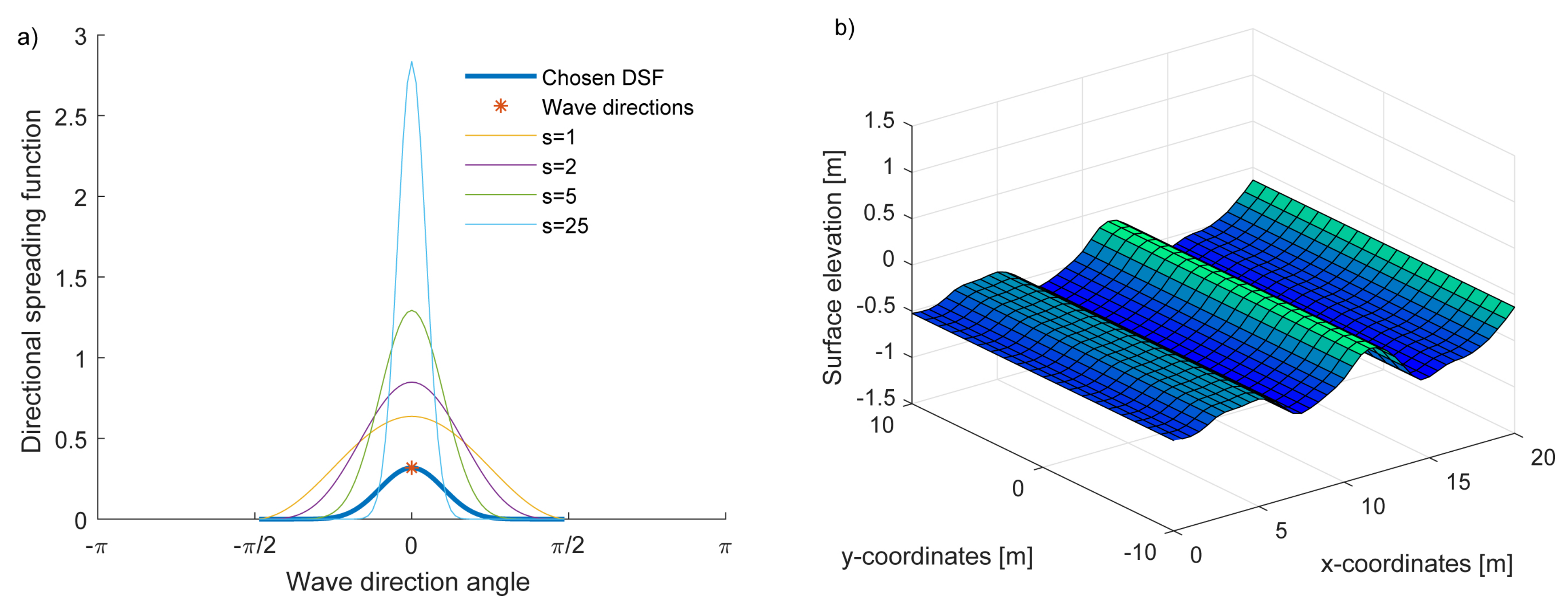
The principal wave direction will be considered here as $\overline{\chi }=0$, i.e., moving along the x-direction. The shape of the directional spreading function for different values of the spreading parameter s is shown in Figure 2. As can be seen from the figure, the higher the spreading parameter, the more energy in the waves is distributed along the principal wave direction.

From Equations (15) and (17), the amplitude function can be also decomposed into a directional independent part and the directional dependent part. However, from Equation (15), only the modulus of the complex amplitude is known, and we add an unknown phase $\phi (\omega ,\chi )$, which is assumed to be uniformly distributed over $(-\pi ,\pi )$,

$$\begin{array}{cc}\hfill A(\omega ,\chi )& =|A(\omega ,\chi )|e^{i\arg \left(A\right(\omega ,\chi \left)\right)}\hfill \\ \hfill & =\sqrt{\frac{S\left(\omega \right)D(\omega ,\chi )}{2d\omega d\chi }}{e}^{i\arg \left(A\right(\omega ,\chi \left)\right)}\hfill \\ \hfill & =|A\left(\omega \right)|\sqrt{D(\omega ,\chi )\frac{1}{d\chi }}{e}^{i\arg \left(A\right(\omega ,\chi \left)\right)}\hfill \\ \hfill & =A\left(\omega \right)\sqrt{D(\omega ,\chi )\frac{1}{d\chi }}{e}^{i\phi (\omega ,\chi )},\hfill \end{array}$$

(25)

where $D(\omega ,\chi )$ is the directional spreading function defined in Equation (21). In this work, we will use incident irregular unidirectional waves for which the surface amplitude $A\left(\omega \right)$ is known, and compute the complex amplitudes for the short-crested waves according to the expression in Equation (25).

In the frequency domain, the surface elevation can be written as the product of the amplitude function and a transfer function $H_m\left(\omega \right)$,

$$\widehat{\eta }(x,y,\omega )=\sum _{m=1}^{M}A(\omega ,{\chi }_m)e^{-ik(xcos{\chi }_m+ysin{\chi }_m)}d\chi =\sum _{m=1}^M\sqrt{D({\chi }_m-\overline{\chi })d\chi }A\left(\omega \right)H_m\left(\omega \right),$$

(26)

where $H_m\left(\omega \right)=e^{-ik(xcos{\chi }_m+ysin{\chi }_m)+i\phi (\omega ,{\chi }_m)}$.

In the time domain, the inverse Fourier transform of the product becomes a convolution

$$\eta (x,y,t)=\sum _{m=1}^M\sqrt{D({\chi }_m-\overline{\chi })d\chi }\eta (0,0,t)\ast h_m\left(t\right),$$

(27)

where $\eta (0,0,t)=\widehat{A\left(\omega \right)}$ is the surface elevation at point $(x,y)=(0,0)$ and $h_m\left(t\right)$ is the inverse Fourier transform of the transfer function $H_m\left(\omega \right)$.

The fluid potential of the incident wave in Equation (10) can be written in the frequency domain as

$${\varphi }_0(x,y)=\sum _{m=1}^M\frac{ig}{\omega }A(\omega ,{\chi }_m){\psi }_0\left(z\right)e^{i[-k(xcos{\chi }_m+ysin{\chi }_m)]}d\chi ,$$

(28)

where ${\psi }_0\left(z\right)$ is the vertical eigenfunction defined as

$${\psi }_0\left(z\right)=\frac{cosh\left(k\right(z+h\left)\right)}{cosh\left(kh\right)}.$$

(29)

Consider now a buoy located at position $(x^i,y^i)$ with local cylindrical coordinates $(r,\theta ,z)$. Due to properties of Bessel functions, the incident fluid potential in Equation (28) can be rewritten in the local coordinate system as

$$\begin{array}{cc}\hfill {\varphi }_0(r,\theta ,z)& =\sum _{m=1}^M\frac{ig}{\omega }A(\omega ,{\chi }_m){\psi }_0\left(z\right)e^{i[-k(x^{i}cos{\chi }_m+y^{i}sin{\chi }_m)]}{e}^{-ikrcos(\theta -{\chi }_m)}d\chi \hfill \\ \hfill & =\sum _{m=1}^M\frac{ig}{\omega }A(\omega ,{\chi }_m){\psi }_0\left(z\right)e^{-ik(x^{i}cos{\chi }_m+y^{i}sin{\chi }_m)}d\chi \sum _{n=-\infty }^{\infty }{(-i)}^n{J}_n\left(kr\right)e^{in(\theta -{\chi }_m)}\hfill \\ \hfill & =\sum _{n=-\infty }^{\infty }{Z}_0\left(z\right)\underset{A_{0n}^i}{\underbrace{\left[\sum _{m=1}^M\frac{ig}{\omega }A(\omega ,{\chi }_m)e^{-ik(x^{i}cos{\chi }_m+y^{i}sin{\chi }_m)}\frac{{(-i)}^n}{Z_0\left(0\right)}{e}^{-in{\chi }_m}d\chi \right]}}{J}_n\left(kr\right)e^{in\theta }\hfill \\ \hfill & =\sum _{n=-\infty }^{\infty }{Z}_0\left(z\right)A_{0n}^i{J}_n\left(kr\right)e^{in\theta },\hfill \end{array}$$

(30)

where $Z_0\left(z\right)$ is the normalized vertical eigenfunction satisfying ${\psi }_0\left(z\right)=Z_0\left(z\right)/Z_0\left(0\right)$ and $J_n\left(kr\right)$ are oscillating Bessel functions.

2.2.3. Multiple Scattering

Any point in the global coordinate system can be written in terms of the local cylindrical coordinate system defined at the origin $(x^i,y^i)$ at each buoy as $(x,y,z)=(x^i+rcos\theta ,y^i+rsin\theta ,z)$. At each buoy, the fluid domain is divided into an interior region I beneath the buoy and an exterior region II outside $r>R^i$ (see Figure 1). By separation of variables, a solution to the Laplace equation and the linear boundary constraints at the free surface, the seabed and at the buoy surfaces can be found for the two fluid domains on the general form

$$\begin{array}{cc}\hfill {\varphi }^{i\left(\mathrm{I}\right)}& =\frac{V^i}{2L^i}({(z+h)}^2-\frac{r^2}{2})+\sum _{n=-\infty }^{\infty }\left[{\gamma }_{m0}^i{\left(\frac{r}{R^i}\right)}^{|n|}+\sum _{m=1}^{\infty }{\gamma }_{mn}^{i}cos\left({\lambda }_m^i(z+h)\right)\frac{I_n\left({\lambda }_m^{i}r\right)}{I_n\left({\lambda }_m^i{R}^i\right)}\right]e^{in\theta }\hfill \end{array}$$

(31)

$$\begin{array}{cc}\hfill {\varphi }^{i\left(\mathrm{II}\right)}& =\sum _{n=-\infty }^{\infty }\left[{\alpha }_{0n}^i{Z}_0\left(z\right)\frac{H_n\left(kr\right)}{H_n\left(k{R}^i\right)}+\sum _{m=1}^{\infty }{\alpha }_{mn}^i{Z}_m\left(z\right)\frac{K_n\left(k_{m}r\right)}{K_n\left(k_m{R}^i\right)}\right]e^{in\theta },\hfill \end{array}$$

(32)

where I/II define the interior/exterior regions and $L^i=h-d^i$ where h is the water depth and $d^i$ the individual drafts of the buoys. The wave number $k_0=-ik$ is a solution to the dispersion relation ${\omega }^2=gktanh\left(kh\right)$, and the Hankel functions $H_n\left(kr\right)$ correspond to propagating modes. The wave numbers $k_m$, $m>0$ are consecutive roots to the dispersion relation ${\omega }^2=-g{k}_{m}tan\left(k_{m}h\right)$, and the Bessel functions $K_n\left(k_{m}r\right)$ correspond to evanescent modes. $I_n\left({\lambda }_{m}r\right)$ are modified Bessel functions with argument ${\lambda }_m^i=m\pi /L^i$.

The term proportional to the velocity $V^i$ in the potential in the interior domain is required to satisfy the inhomogeneous boundary constraint at the body surface of the oscillating buoy. If the buoy is stationary, its velocity vanishes $V^i=0$, and the potential in the interior region only contains its second, homogeneous term.

Solving the multiple scattering problem is essentially a matter of finding the unknown coefficients in expressions (31) and (32) by requiring continuity of the potentials and their derivatives at the domain boundaries $r=R^i$. The problem can be solved with incident waves and oscillating buoys occurring simultaneously, but for clarity will here be solved as two separate problems, where, in the scattering problem, the buoys are held fixed and there are incident waves, and in the radiation problem the buoys are free to oscillate, but there are no incident waves. The derivation follows the same procedure as shown in [16,28], and the reader is referred to those references for further details.

Scattering Problem

Consider incident short-crested waves as described by the fluid potential in Equation (30) and let the buoys be fixed, with zero velocity $V^i=0$. The potential in the exterior domain of any buoy will be a superposition of incident wave ${\varphi }_0^i$, scattered waves ${\varphi }_S^i$, and incoming waves that are scattered off the other buoys ${\varphi }_S^j$, $j\ne i$,

$${\varphi }^{i,\mathrm{II}}={\varphi }_0^i+{\varphi }_S^i+\sum _{j\ne i}{\varphi }_S^j{|}_i.$$

(33)

By using Graf’s addition theorems for Bessel functions, the outgoing waves from one buoy can be written as an incoming wave in the local coordinates of another cylinder as

$${\varphi }_S^j{|}_i=\sum _{n=-\infty }^{\infty }\left[Z_0\left(z\right)J_n\left(kr\right)\sum _{l=-\infty }^{\infty }{T}_{0ln}^{ij}{\alpha }_{0l}^j+\sum _{m=1}^{\infty }{Z}_m\left(z\right)\frac{I_n\left(k_{m}r\right)}{I_n\left(k_{m}R\right)}\sum _{l=-\infty }^{\infty }{T}_{mln}^{ij}{\alpha }_{ml}^j\right]e^{in{\theta }_i},$$

(34)

where the expressions for $T^{ij}=T_{mln}^{ij}$ are given in the Appendix. Continuity between the interior (31) and exterior solutions (32) and their derivatives along the boundaries $r=R^i$ between the interior and exterior domains implies the infinite system of equations

$$\sum _{m=0}^{\infty }{D}_{smn}^i{\alpha }_{mn}^i=-\sum _{m=0}^{\infty }{\tilde{D}}_{smn}^i\left(A_{0n}^i{\delta }_{m0}+\sum _{j\ne i}\sum _{l=-\infty }^{\infty }{T}_{mln}^{ij}{\alpha }_{ml}^j\right),$$

(35)

together with an expression for the coefficients $\gamma$ in the interior solution in terms of the coefficients $\alpha$, given in Equation (A5). The matrices D, $\tilde{D}$ and their components are defined in the appendix.

To solve for the unknown coefficients ${\alpha }^i$ from Equation (35), we truncate the infinite sums at the vertical cut-off ${\mathsf{\Lambda }}_z$ for the vertical sums ${\sum }_m{Z}_m\left(z\right)$ and the angular cut-off ${\mathsf{\Lambda }}_{\theta }$ for the angular sums ${\sum }_n{e}^{in\theta }$. The system of equations take the form

$$\left[\begin{array}{cccc}1& -B^1{T}^{12}& \cdots & -B^1{T}^{1N}\\ -B^2{T}^{21}& 1& \cdots & -B^2{T}^{2N}\\ ⋮& ⋮& \ddots & ⋮\\ -B^N{T}^{N1}& -B^N{T}^{N2}& \cdots & 1\end{array}\right]\left[\begin{array}{c}{\alpha }^1\\ {\alpha }^2\\ ⋮\\ {\alpha }^N\end{array}\right]=\left[\begin{array}{c}{B}^1{A}_{0n}^1\\ B^2{A}_{0n}^2\\ ⋮\\ B^N{A}_{0n}^N\end{array}\right],$$

(36)

where $B^i=-{\left[D^i\right]}^{-1}{\tilde{D}}^i$ is the single-body diffraction matrix and $A_{0n}^i$ is defined for the incident, short-crested waves as in Equation (30). The matrix on the left-hand side is called the diffraction matrix. The diagonal entries are identity matrices, and the non-diagonal entries $B^i{T}^{ij}$ account for the hydrodynamical multiple scattering interactions. Neglecting the multiple scattering would result in the diffraction matrix being the identity matrix. Solving the equation in (36) is the computationally most extensive part of the computation, as the diffraction matrix is a large, quadratic matrix of size $N({\mathsf{\Lambda }}_z+1)(2{\mathsf{\Lambda }}_{\theta }+1)$.

When the scattering coefficients $\alpha$ in the diffraction potential in the exterior domain have been solved from Equation (36), the coefficients $\gamma$ in the potential in the interior domain can be found from Equation (A5), and the heave excitation force can be computed from Equation (11) as

$$F_{\mathrm{exc}}^i\left(\omega \right)=2\pi i\omega \rho \left[{\gamma }_{00}^i\frac{{\left(R^i\right)}^2}{2}+2R^i\sum _{m=1}^{{\mathsf{\Lambda }}_z}{\gamma }_{m0}^i\frac{{(-1)}^m}{{\lambda }_m^i}\frac{I_1\left({\lambda }_m^i{R}^i\right)}{I_0\left({\lambda }_m^i{R}^i\right)}\right].$$

(37)

Radiation Problem

The radiation problem follows the same procedure as the scattering problem, but solves the problem when there are no incident waves and the buoys are free to oscillate with independent velocities $V^i$.

The potential in the exterior domain of any buoy will be a superposition of radiated and scattered waves of the own body, and incoming waves that are scattered and radiated off the other buoys,

$${\varphi }^{i,\mathrm{II}}={\varphi }_R^i+{\varphi }_S^i+\sum _{j\ne i}\left({\varphi }_R^j+{\varphi }_S^j\right){|}_i.$$

(38)

By using Graf’s addition theorems for Bessel functions, the outgoing waves from one buoy can be written as an incoming wave in the local coordinates of another cylinder as in (34), and again continuity between the fluid domains implies the infinite system of equations

$$\sum _{m=0}^{\infty }{D}_{smn}^i{\alpha }_{mn}^i=-\sum _{m=0}^{\infty }{\tilde{D}}_{smn}^i\left(\sum _{j\ne i}\sum _{l=-\infty }^{\infty }{T}_{mln}^{ij}{\alpha }_{ml}^j\right)-V^i{R}_s^i{\delta }_{0n},$$

(39)

together with Equation (A5), where $R_s^i$ is the radiation vector defined in the appendix and $\alpha$ contains coefficients for both the scattered and radiated waves in (38). As in the scattering problem, the infinite sums are truncated to obtain a finite system of equations

$$\left[\begin{array}{cccc}1& -B^1{T}^{12}& \cdots & -B^1{T}^{1N}\\ -B^2{T}^{21}& 1& \cdots & -B^2{T}^{2N}\\ ⋮& ⋮& \ddots & ⋮\\ -B^N{T}^{N1}& -B^N{T}^{N2}& \cdots & 1\end{array}\right]\left[\begin{array}{c}{\alpha }^1\\ {\alpha }^2\\ ⋮\\ {\alpha }^N\end{array}\right]=\left[\begin{array}{c}{V}^1{B}_R^1\\ V^2{B}_R^2\\ ⋮\\ V^N{B}_R^N\end{array}\right],$$

(40)

where $B_R^i={\left[D^i\right]}^{-1}{R}_s^i$. When the scattering and radiation coefficients $\alpha$ have been solved from Equation (40), the coefficients $\gamma$ in the potential in the interior domain can be found from Equation (A5), and the heave radiation force can be computed from Equation (12) as

$$F_{\mathrm{rad}}^i\left(\omega \right)=2\pi i\omega \rho \left[\frac{V^i{L}^i}{4}\left({\left(R^i\right)}^2-\frac{{\left(R^i\right)}^4}{4{\left(L^i\right)}^2}\right)+{\gamma }_{00}^i\frac{{\left(R^i\right)}^2}{2}+2R^i\sum _{m=1}^{{\mathsf{\Lambda }}_z}{\gamma }_{m0}^i\frac{{(-1)}^m}{{\lambda }_m^i}\frac{I_1\left({\lambda }_m^i{R}^i\right)}{I_0\left({\lambda }_m^i{R}^i\right)}\right].$$

(41)

There is an implicit velocity dependence in the coefficients $\gamma$ that can be factored out, and the radiation force can be written in terms of added mass and radiation damping as

$$F_{\mathrm{rad}}^i\left(\omega \right)=\sum _{i=1}^N{\left[i\omega m_{\mathrm{rad}}-B\right]}_j^i{V}^j.$$

(42)

2.3. Numerical Implementation

To transform Equation (35) to a finite system of linear equations, the vertical and angular cut-offs have been chosen as ${\mathsf{\Lambda }}_z=20$ (index $s,m=1,\dots ,20$) and ${\mathsf{\Lambda }}_{\theta }=3$ (index $l,n=-3,-2,\dots ,2,3$). In [28], these cut-off values were shown to produce results with a high accuracy as compared to computations performed with the state-of-art software WAMIT (version 7.062, Massachusetts Institute of Technology, MA, USA). The theory and equations described in Section 2.1 and Section 2.2 have been implemented and solved in a MATLAB (version R2017a, MathWorks Inc., MA, USA) script.

Although the method allows the use of an interaction distance cut-off [28] to speed up the computations with attained high accuracy, in this paper, that option has not been used, and full hydrodynamical interaction is computed between all devices.

The water depth has been chosen to constant $h=25$ m, based on the depth at the test site Lysekil on the west coast of Sweden. In this paper, the dimensions of the WECs in the park have been chosen constant and equal for all WECs. The buoy radius has been chosen to $R=3$ m, the draft to $d=0.5$ m and the power take-off damping to $\mathsf{\Gamma }=200$ kNs/m.

The incident short-crested waves are computed as described in Section 2.2.2, where the incident long-crested waves with amplitude $A\left(\omega \right)$ is the Fourier transform of the incident long-crested waves at the origin, $\eta (0,0,t)$. The time-series of incident waves $\eta (0,0,t)$ is measured by a Datawell Waverider buoy installed at the Lysekil test site, Sweden. One hour of incident wave data has been used, which was measured on 1 January 2015 with a sampling frequency of 2.56 Hz. The sea state is characterized by a significant wave height of $H_s=1.88$ m and an energy period of $T_e=5.98$ s.

3. Results and Discussion

3.1. Irregular, Short-Crested Waves

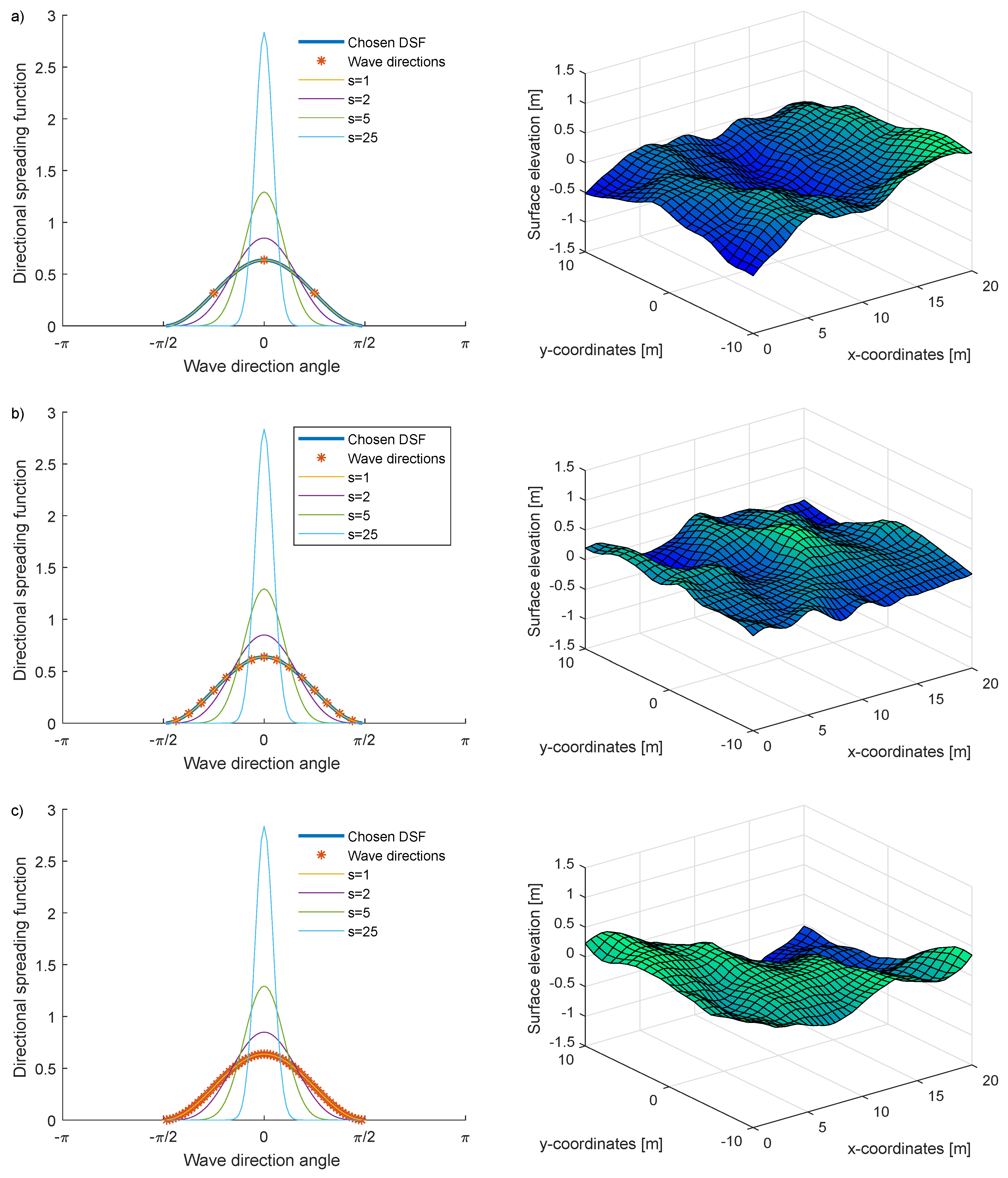
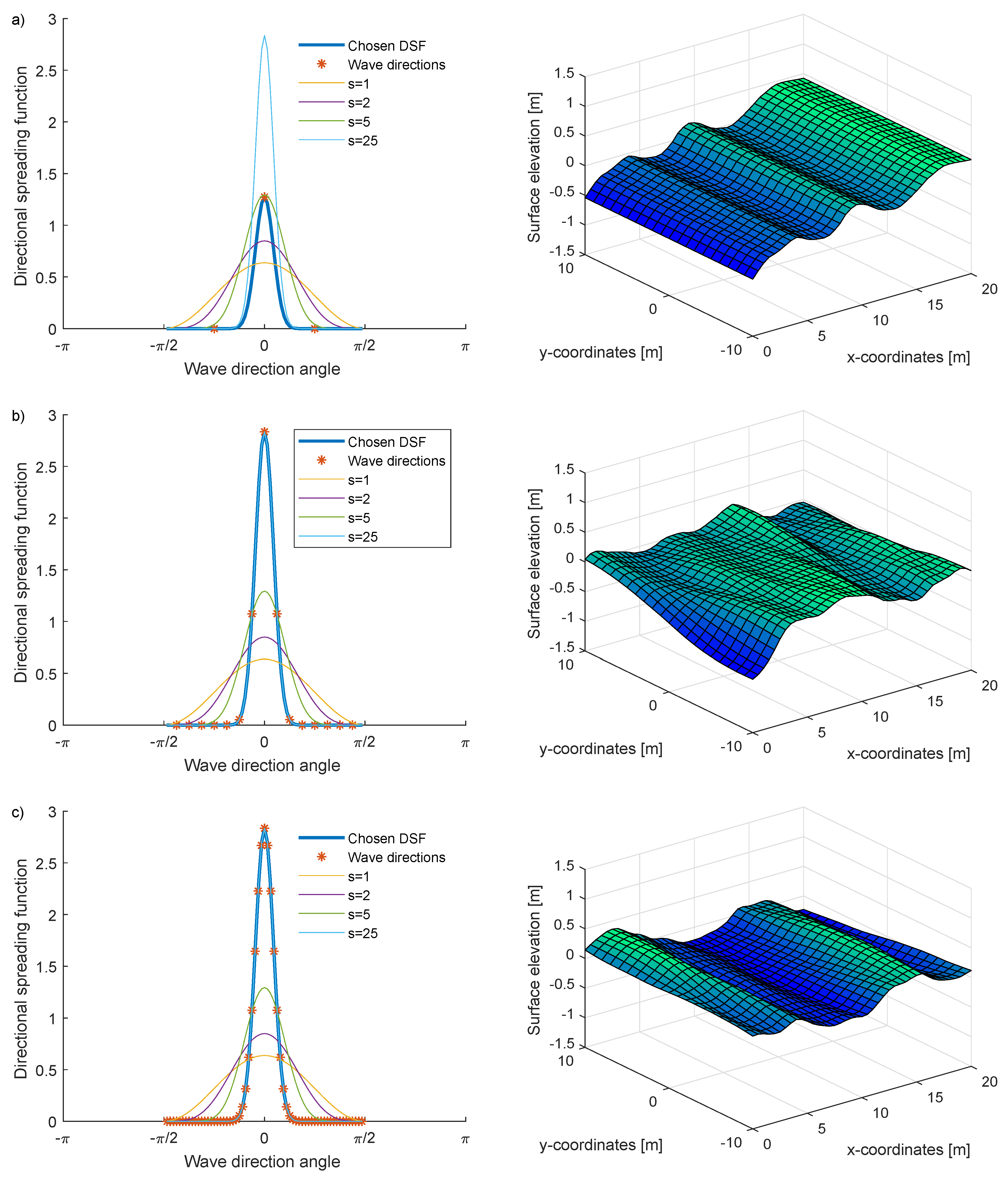
The surface elevation in time domain is plotted at the same instant in time for different values of the spreading parameter s and different number of wave directions in Figure 2, Figure 3, Figure 4 and Figure 5, together with the corresponding directional spreading function. As is expected from the form of the directional spreading function and clear from the figures, a larger spreading parameter s implies that more energy in the waves is propagating along the principal wave direction, with the asymptotic state being a unidirectional wave. Hence, the short-crested wave in Figure 5a with $s=25$ takes a similar form as the long-crested, unidirectional wave in Figure 2. In Figure 3, Figure 4 and Figure 5, the spreading parameter is kept constant to $s=1$, $s=5$ and $s=25$, respectively, while the number of wave directions is increased from three in subfigures (a), 15 in subfigures (b) and 63 in subfigures (c).

Hence, the upper rows, i.e., Figure 3a, Figure 4a and Figure 5a all have three wave directions but increasing spreading parameter from $s=1$ to $s=25$, and equivalently the Figure 3b, Figure 4b and Figure 5b share the same 15 wave directions but increasing spreading parameter, and Figure 3c, Figure 4c and Figure 5c all have 63 wave directions but increasing spreading parameter. As can be seen from the figures, not only the spreading parameter affects the surface elevation, but also the number of wave directions. The fewer wave directions, the more the waves resemble a long-crested, unidirectional wave, which should be expected.

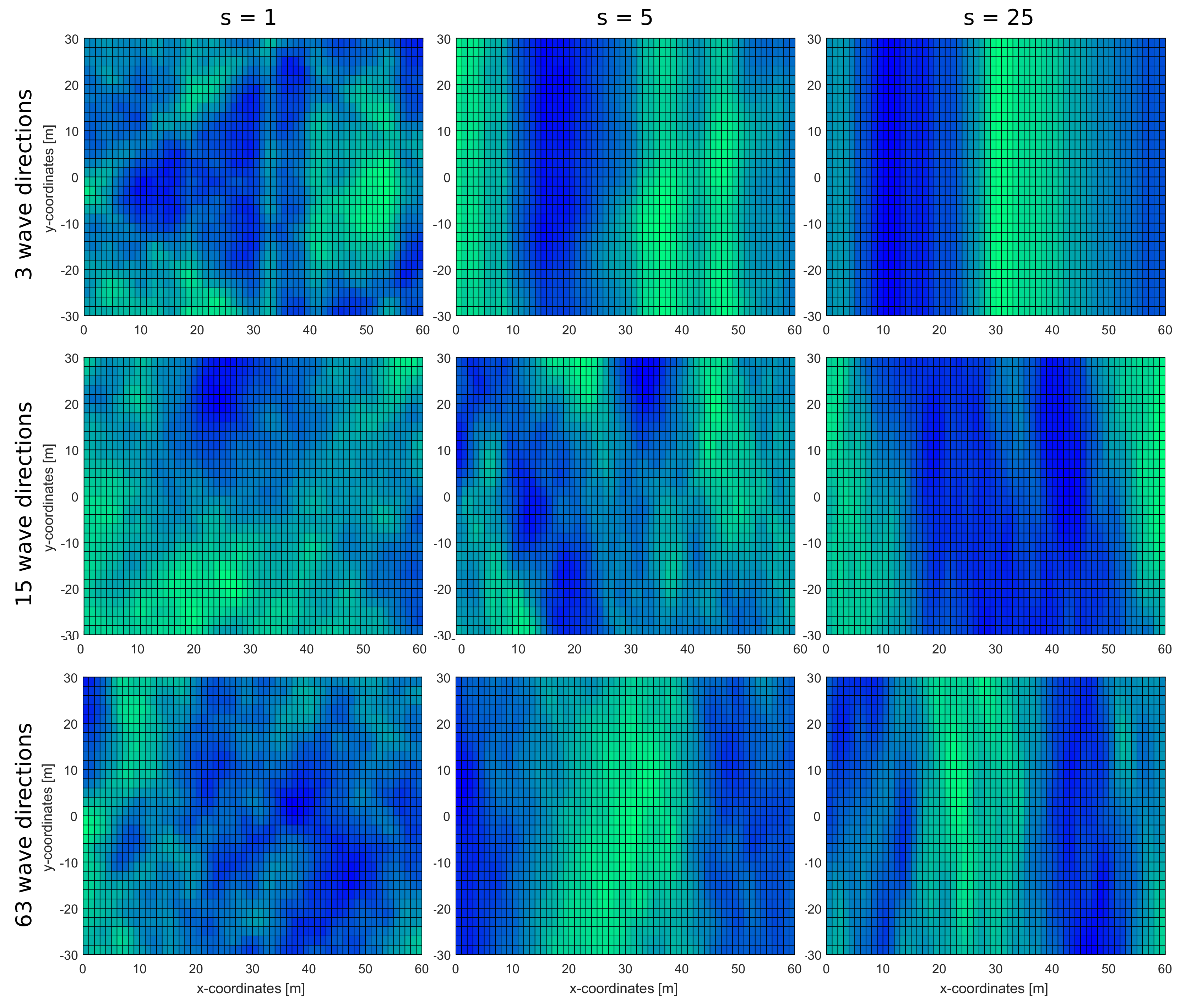
To analyse the effect of wave directions and spreading parameter even further, the surface elevations for all cases is shown in Figure 6. Here, the spreading parameter increases with the columns, with $s=1$ in the left column, $s=5$ in the middle and $s=25$ in the right column, and the number of wave directions increases with the rows, with three wave directions in the top row, 15 in the middle and 63 wave directions in the bottom row. In the upper left figure, the three wave directions $\{-\pi /4,0,\pi /4\}$ are clearly distinguishable, whereas this is more vague in the other cases. As can be seen in the figures, the fewer wave directions (upper row) and the higher spreading parameter (right column), the more the resulting waves resemble long-crested waves.

3.2. Wave Energy Arrays in Short-Crested Waves

Due to the random phase in Equation (25), different short-crested waves will be generated in each simulation. The random phase is a function of both the wave direction and the frequency, hence all wave direction and wave frequency components of the composed waves will receive independent phases each time. For an evaluation of the wave energy park performance in short-crested waves, the simulations should be carried out a number of times with different random phases, and the average taken.

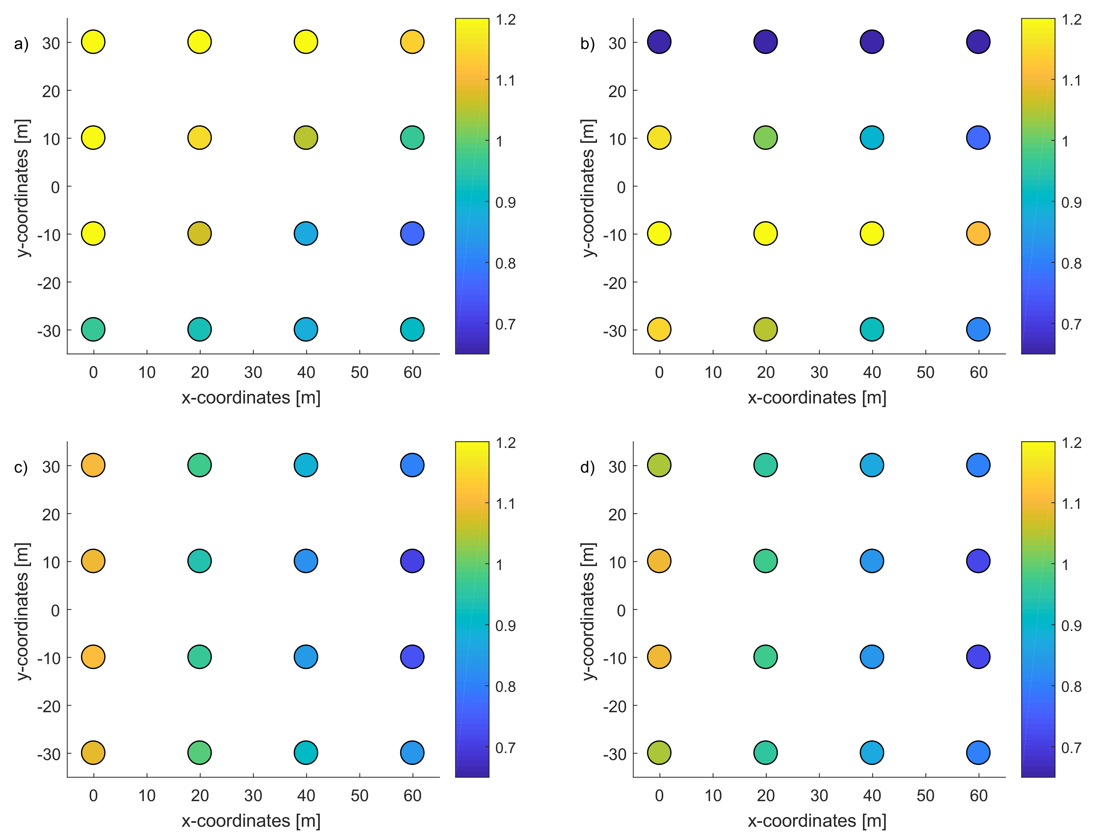
In Figure 7a,b, two different simulations of park performance in short-crested waves are shown. The park consists of 16 WECs in a gridded layout with 20 m separation distance. In the figure, the color of each WEC shows the normalized energy absorption $q^i$ of Equation (8), i.e., value $q^i>1$ implies that the WEC absorbs more wave power than it would in isolation at the origin. As can be seen from Figure 7a,b, the result differs for two different random phases in the short-crested waves; there is no clear pattern of wave shadowing or constructive/destructive interactions. In Figure 7c, an average of 50 simulations such as the ones shown in Figure 7a,b is shown. When an average is taken, a pattern emerges, and it is clear that wave shadowing occurs: the first row at $x=0$ m absorbs more power than the second row at $x=20$ m, and so on. The case of long-crested, unidirectional waves is shown in Figure 7d, where as expected the absorbed power by each WEC decreases strictly with the number of rows perpendicular to the incident wave direction. One can observe that when an average over a multiple of short-crested waves with different random phases is taken, the result converges to the long-crested wave case.

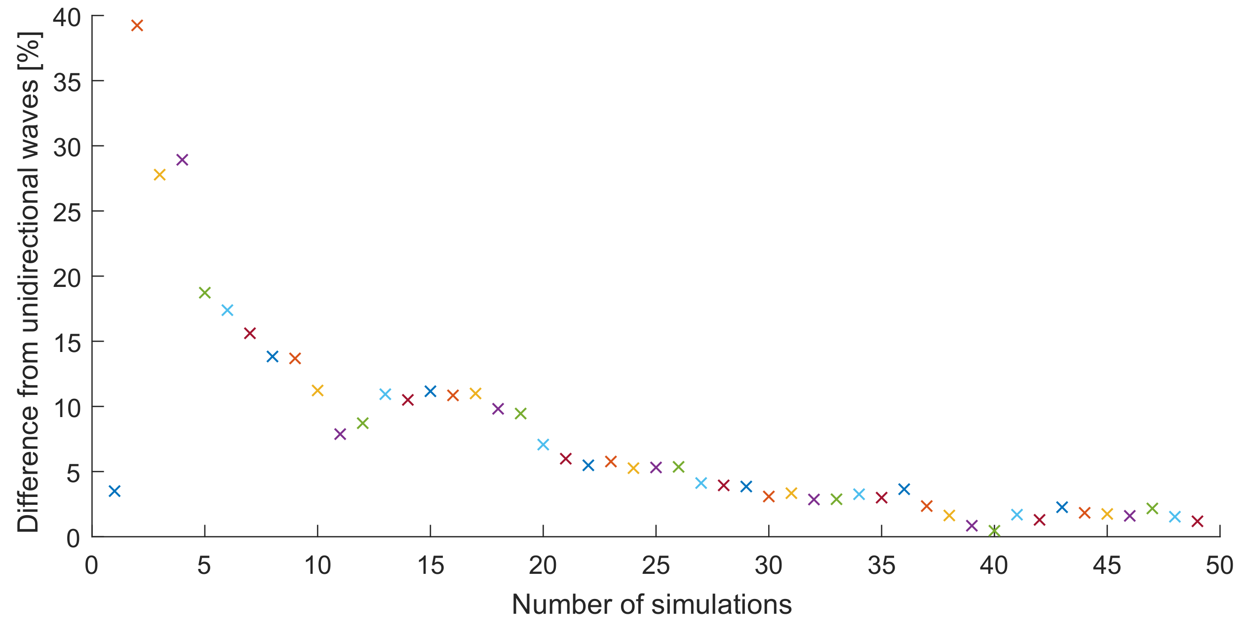
The convergence of the normalized energy absorption is shown in more detail in Figure 8. Here, for each simulation number S, the average of the ratio of the individual normalized energy absorption in short-crested and long-crested waves is computed, and the average is taken over all the simulations $s=1,\dots ,S$,

$$\frac{1}{S}\sum _{s=1}^S\left(\frac{1}{N}\sum _{i=1}^N\frac{q_{\mathrm{short},s}^i}{q_{\mathrm{long},s}^i}\right).$$

(43)

As can be seen from the figure, the power absorption for the parks in short-crested waves converges to the unidirectional case; after 30 simulations with random phases, the difference is less than 5% and, after 50 simulations (shown in Figure 7c), the difference is 1.6%.

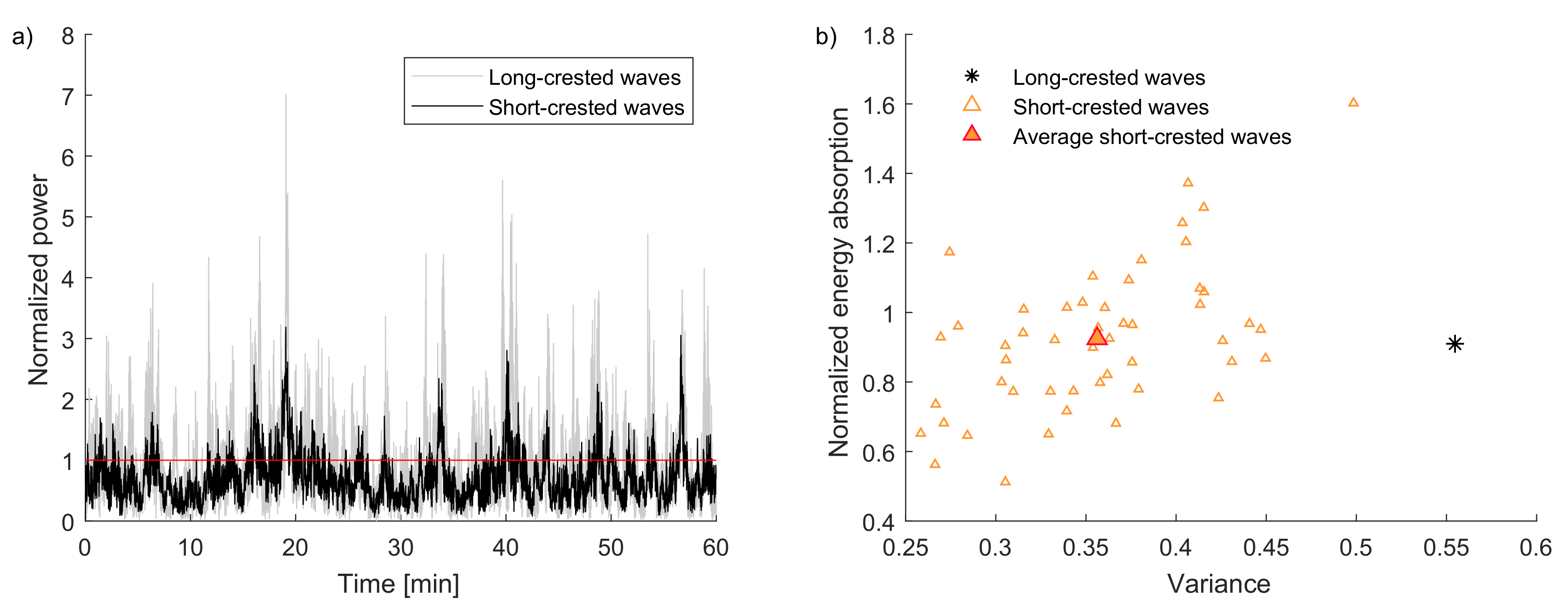
In Figure 9a, the total instant power of a park with 16 wave energy devices (with park layout shown in Figure 7) is shown both in long-crested and short-crested waves. The power has been divided by the average power of a single device in isolation times the number of devices in a park. As is clear from the figure, the power output of the park in these short-crested waves have smaller power peaks than in the long-crested waves. This is a desired behaviour as connection to the electricity grid requires a good electricity quality with small power fluctuations. This is also an expected result, since the WECs in the same row perpendicular to the unidirectional wave direction will be excited simultaneously by the incident long-crested waves, whereas this does not happen in short-crested waves. Nevertheless, although it is an expected result, it is still important to quantify the reduction of the power fluctuations in short-crested waves, so that realistic values are used as design parameters for the electrical system of a park. A useful measure of the power fluctuations in a park is given by the variance (6). However, low fluctuations is only one measure of good park performance; in addition, large energy absorption is required, which can be quantified in terms of the normalized energy absorption (7). An optimal park will have a high energy absorption and low power fluctuations, simultaneously.

To evaluate this, both the variance and the energy absorption have been plotted in Figure 9b. Ideal performance would end up in the upper left part of the figure, with high energy absorption and low variance. The performance in long-crested waves is shown by a black asterisk, and the performance in short-crested waves is shown by orange triangles, one for each simulation (corresponding to different random phases). The average of all the short-crested waves is shown with a larger filled triangle. As can be seen from the figure, the energy absorption in short-crested waves has a significantly lower variance, i.e., the power fluctuations are significantly lower. The spread in normalized energy absorption is large and ranges from 0.512 to 1.60, but the average of all simulations in short-crested waves has a normalized energy absorption of 0.925, which is similar to and even slightly higher than the value in long-crested waves, $q=0.910$. To summarize, the power fluctuations are lower in short-crested waves, and the energy absorption is comparable. In short, the performance is better in short-crested waves as compared to long-crested waves.

3.3. Effect of Varying Wave Directions and Spreading Parameter

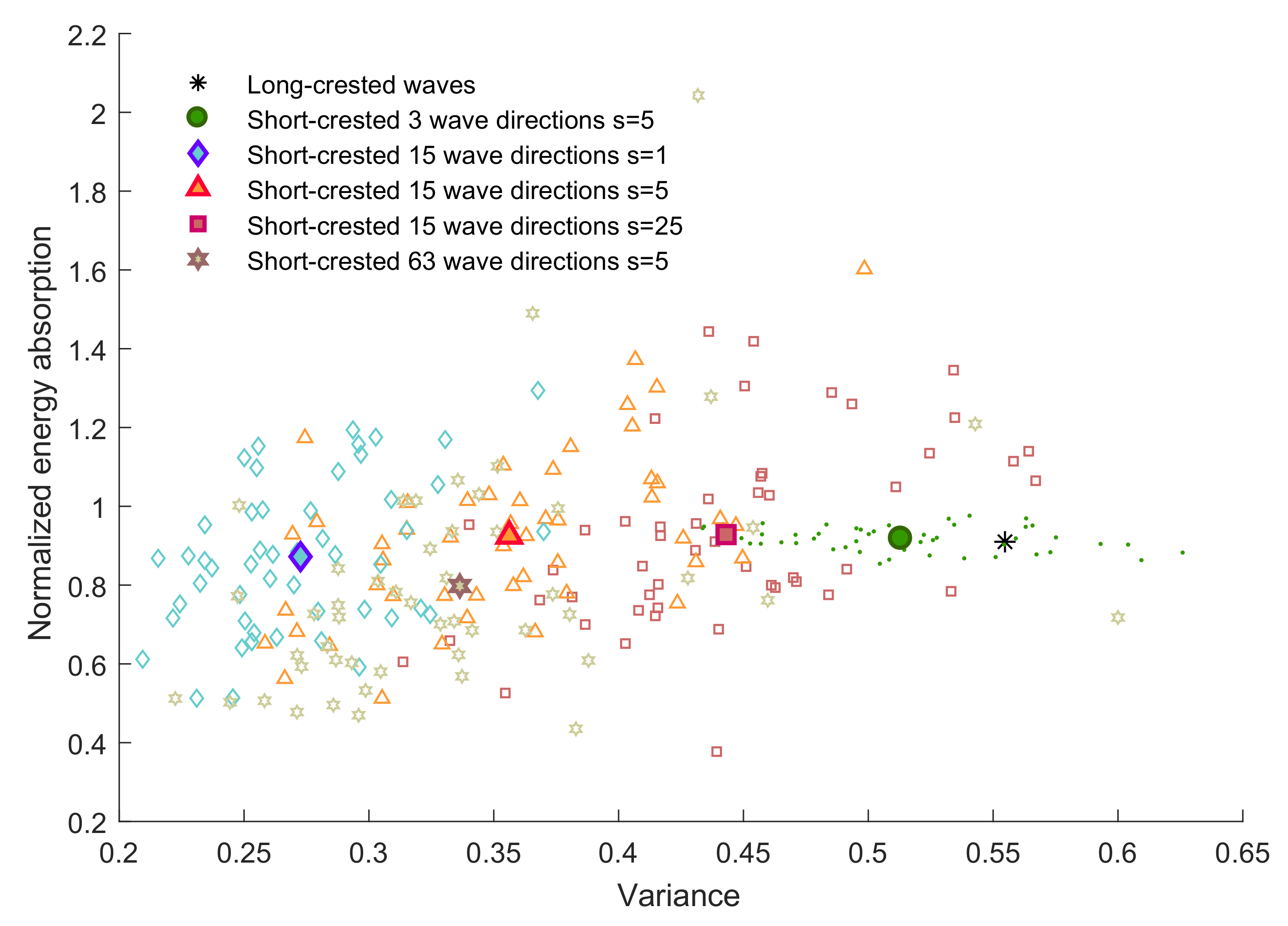
In Section 3.2, results were presented for short-crested waves with 15 wave directions and spreading parameter $s=5$, corresponding to directional wave spectrum and corresponding surface elevation shown in Figure 4b. In this section, we evaluate the performance in short-crested waves of different number of wave directions and different spreading parameter values. In Figure 10, the extension of Figure 9b is shown for a larger class of short-crested waves. Short-crested waves with spreading parameter $s=5$ consisting of 3, 15 and 63 wave directions (corresponding to the waves in Figure 4) and short-crested waves with spreading parameter $s=1$, $s=5$ and $s=25$ consisting of waves with 15 wave directions (corresponding to the waves in Figure 3b, Figure 4b and Figure 5b) have been considered.

From Figure 10, it is clear that all short-crested waves show a similar performance with lower power fluctuations and similar energy absorption, as compared to the performance in long-crested waves. The more the short-crested waves tend towards long-crested waves (i.e., the fewer the wave directions and the higher the spreading parameter, as discussed in Section 3.1 and shown in Figure 3 , Figure 4, Figure 5 and Figure 6), the more the resulting performance converges to the unidirectional case. An ideal wave energy park would have low fluctuations and high power absorption and end up in the upper left corner. The simulations show that the spread in the results is large, but when an average is taken over all 50 simulations with different random phases, the trend is clear; the parks in short-crested waves have lower fluctuations, and no significant change in power absorption as compared to long-crested waves.

4. Conclusions

Realistic ocean waves can be short-crested and consist of irregular waves travelling in several directions simultaneously. However, most studies on wave energy parks have been carried out in long-crested, unidirectional waves. The few that have considered short-crested waves have indicated that the performance of the wave energy parks might be different in short-crested as compared to long-crested waves, and that the subject needs further study.

In this paper, theory for including short-crested (multidirectional) irregular waves in a multiple scattering method has been developed and implemented in a semi-analytical MATLAB code. The directional dependence of the waves is described by a directional spreading function, and the impact of different spreading parameters and number of wave directions has been analysed. The short-crested waves converge to unidirectional, long-crested waves with increasing spreading parameter and decreasing number of wave directions.

The model has then been used to evaluate the performance of wave energy parks in short-crested waves. The performance is evaluated according to two important parameters: the energy absorption and the power fluctuations. An optimal wave energy park will have a large energy absorption but low power fluctuations, in order to ensure a good electricity quality to the electric grid.

Since all the wave direction components have different random phases, each simulation will produce different results due to the different waves produced at each location in the park. A convergence study was performed and showed that the energy absorption in short-crested waves converges to the long-crested case; an average of 50 simulations differed only 1.6% in energy absorption from the long-crested waves case. The power fluctuations, however, are clearly lower in the short-crested waves. The conclusion, therefore, is that the performance of wave energy parks in short-crested waves can be better than what has been anticipated from simulations using long-crested waves, with similar energy absorption and lower power fluctuations.

References

- Budal, K. Theory for absorption of wave power by a system of interacting bodies. J. Ship Res. 1977, 21, 248. [Google Scholar]
- Falnes, J. Radiation impedance matrix and optimum power absorption for interacting oscillators in surface waves. Appl. Ocean Res. 1980, 2, 75. [Google Scholar] [CrossRef]
- Thomas, G.; Evans, D. Arrays of three-dimensional wave energy absorbers. J. Fluid Mech. 1981, 108, 67–88. [Google Scholar] [CrossRef]
- Bozzi, S.; Giassi, M.; Miquel, A.; Antonini, A.; Bizzozero, F.; Gruosso, G.; Archetti, R.; Passoni, G. Wave energy farm design in real wave climates: The Italian offshore. Energy 2017, 122, 378–389. [Google Scholar] [CrossRef]
- Penalba, M.; Touzón, I.; Lopez-Mendia, J.; Nava, V. A numerical study on the hydrodynamic impact of device slenderness and array size in wave energy farms in realistic wave climates. Ocean Eng. 2017, 142, 224–232. [Google Scholar] [CrossRef]
- Xu, D.; Stuhlmeier, R.; Stiassnie, M. Harnessing wave power in open seas II: Very large arrays of wave-energy converters for 2D sea states. J. Ocean Eng. Mar. Energy 2017, 3, 151–160. [Google Scholar] [CrossRef]
- Tay, Z.; Venugopal, V. Hydrodynamic interactions of oscillating wave surge converters in an array under random sea state. Ocean Eng. 2017, 145, 382–394. [Google Scholar] [CrossRef]
- López-Ruiz, A.; Bergillos, R.; Raffo-Caballero, J.; Ortega-Sánchez, M. Towards an optimum design of wave energy converter arrays through an integrated approach of life cycle performance and operational capacity. Appl. Energy 2018, 209, 20–32. [Google Scholar] [CrossRef]
- Fàbregas Flavià, F.; McNatt, C.; Rongère, F.; Babarit, A.; Clément, A. A numerical tool for the frequency domain simulation of large arrays of identical floating bodies in waves. Ocean Eng. 2018, 148, 299–311. [Google Scholar] [CrossRef]
- Thorburn, K.; Leijon, M. Farm size comparison with analytical model of linear generator wave energy converters. Ocean Eng. 2007, 34, 908–916. [Google Scholar] [CrossRef]
- Folley, M.; Whittaker, T. The effect of sub-optimal control on the spectral wave climate on the performance of wave energy converter arrays. Appl. Ocean Res. 2009, 31, 260–266. [Google Scholar] [CrossRef]
- Rahm, M.; Svensson, O.; Boström, C.; Waters, R.; Leijon, M. Experimental results from the operation of aggregated wave energy converters. Renew. Power Gener. IET 2012, 6, 149–160. [Google Scholar] [CrossRef]
- Child, B.; Laporte Weywada, P. Verification and validation of a wave farm planning tool. In Proceedings of the 10th EWTEC Conference, Aalborg, Denmark, 2–5 September 2013. [Google Scholar]
- Göteman, M.; Engström, J.; Eriksson, M.; Isberg, J.; Leijon, M. Methods of reducing power fluctuations in wave energy parks. J. Renew. Sustain. Energy 2014, 6, 043103. [Google Scholar] [CrossRef]
- Giassi, M.; Göteman, M.; Thomas, S.; Engström, J.; Eriksson, M.; Isberg, J. Multi-Parameter Optimization of Hybrid Arrays of Point Absorber Wave Energy Converters. In Proceedings of the 12th European Wave and Tidal Energy Conference (EWTEC), Cork, Ireland, 27 August–1 September 2017. [Google Scholar]
- Göteman, M. Wave energy parks with point-absorbers of different dimensions. J. Fluids Struct. 2017, 74, 142–157. [Google Scholar] [CrossRef]
- Borgarino, B.; Babarit, A.; Ferrant, P. Impact of wave interactions effects on energy absorption in large arrays of wave energy converters. Ocean Eng. 2012, 41, 79–88. [Google Scholar] [CrossRef]
- Engström, J.; Eriksson, M.; Göteman, M.; Isberg, J.; Leijon, M. Performance of a large array of point-absorbing direct-driven wave energy converters. J. Appl. Phys. 2013, 114, 204502. [Google Scholar] [CrossRef]
- Sjolte, J.; Tjensvoll, G.; Molinas, M. Power collection from wave energy farms. Appl. Sci. 2013, 3, 420–436. [Google Scholar] [CrossRef]
- Sarkar, D.; Renzi, E.; Dias, F. Wave farm modelling of oscillating wave surge converters. Proc. R. Soc. A 2014, 470, 20140118. [Google Scholar] [CrossRef] [Green Version]
- Göteman, M.; Engström, J.; Eriksson, M.; Isberg, J. Optimizing wave energy parks with over 1000 interacting point-absorbers using an approximate analytical method. Int. J. Mar. Energy 2015, 10, 113–126. [Google Scholar] [CrossRef]
- Babarit, A. On the park effect in arrays of oscillating wave energy converters. Renew. Energy 2013, 58, 68–78. [Google Scholar] [CrossRef]
- Dias, F.; Renzi, E.; Gallagher, S.; Sarkar, D.; Wei, Y.; Abadie, T.; Cummins, C.; Rafiee, A. Analytical and computational modelling for wave energy systems: the example of oscillating wave surge converters. Acta Mech. Sin. 2017, 33, 647–662. [Google Scholar] [CrossRef] [PubMed]
- Stratigaki, V.; Troch, P.; Stallard, T.; Forehand, D.; Kofoed, J.; Folley, M.; Benoit, M.; Babarit, A.; Kirkegaard, J. Wave Basin Experiments with Large Wave Energy Converter Arrays to Study Interactions between the Converters and Effects on Other Users in the Sea and the Coastal Area. Energies 2014, 7, 701–734. [Google Scholar] [CrossRef] [Green Version]
- Sun, L.; Zang, J.; Eatock Taylor, R.; Taylor, P. Effects of wave spreading on performance of a wave energy converter. In Proceedings of the 29th International Workshop on Water Waves and Floating Bodies, Osaka, Japan, 30 March–2 April 2014. [Google Scholar]
- Ji, X.; Liu, S.; Bingham, H.; Li, J. Multi-directional random wave interaction with an array of cylinders. Ocean Eng. 2015, 110, 62–77. [Google Scholar] [CrossRef] [Green Version]
- Troch, P.; Beels, C.; De Rouck, J.; De Backer, G. Wake effects behind a farm of wave energy converters for irregular long-crested and short-crested waves. Coast. Eng. Proc. 2011, 1, 53. [Google Scholar] [CrossRef]
- Göteman, M.; Engström, J.; Eriksson, M.; Isberg, J. Fast Modeling of Large Wave Energy Farms Using Interaction Distance Cut-Off. Energies 2015, 8, 13741–13757. [Google Scholar] [CrossRef]
- Giassi, M.; Göteman, M. Layout design of wave energy parks by a genetic algorithm. Ocean Eng. 2018, 154, 252–261. [Google Scholar] [CrossRef]
- Tyrberg, S.; Waters, R.; Leijon, M. Wave Power Absorption as a Function of Water Level and Wave Height: Theory and Experiment. IEEE J. Ocean. Eng. 2010, 35, 558–564. [Google Scholar] [CrossRef]
- Hong, Y.; Eriksson, M.; Boström, C.; Waters, R. Impact of Generator Stroke Length on Energy Production for a Direct Drive Wave Energy Converter. Energies 2016, 9, 730. [Google Scholar] [CrossRef]
- Linton, C.; McIver, P. Handbook of Mathematical Techniques for Wave/Structure Interactions; CRC Press: Boca Raton, FL, USA, 2001. [Google Scholar]
- Cartwright, D. The use of directional spectra in studying output of a wave recorder on a moving ship. In Proceedings of the Ocean Wave Spectra: Proceedings of a Conference, Easton, Maryland, 1–4 May 1963; Prentice-Hall, Inc.: Upper Saddle River, NJ, USA, 1963; pp. 203–218. [Google Scholar]
- Mitsuyasu, H.; Tasai, F.; Suhara, T.; Mizuno, S.; Ohkusu, M.; Honda, T.; Rikiishi, K. Observations of the directional spectrum of ocean WavesUsing a cloverleaf buoy. J. Phys. Oceanogr. 1975, 5, 750–760. [Google Scholar] [CrossRef]
- Falnes, J. Ocean Waves and Oscillating Systems: Linear Interactions Including Wave-Energy Extraction; Cambridge University Press: Cambridge, UK, 2002. [Google Scholar]
Figure 1.
Illustration of the fluid domain of the wave energy park. Each wave energy converter is characterized by an individual radius and draft for the float and a power take-off damping of the generator. The fluid domain is divided into interior domains I for each float and exterior domain II.
Figure 2.
(a) Directional spreading function and (b) surface elevation of a long-crested, unidirectional wave, to be compared against the short-crested waves in Figure 3, Figure 4 and Figure 5. For the case of only one wave direction , the value of the spreading parameter is irrelevant as for any values of s. The factor in Equation (24) equals in the case of a single wave direction, which guarantees normalization in Equation (18).
Figure 3.
Directional spreading function in Equation (21) for and increasing wave directions from 3, 15 and 63, as shown in the directional spreading function plots. A time instant of the surface elevation is shown to the right. (a) three wave directions with ; (b) 15 wave directions with ; (c) 63 wave directions with .
Figure 4.
Directional spreading function in Equation (21) for spreading parameter increasing wave directions from 3, 15 and 63, as shown in the directional spreading function plots. A time instant of the surface elevation is shown to the right. (a) three wave directions with ; (b) 15 wave directions with ; (c) 63 wave directions with .
Figure 5.
Directional spreading function in Equation (21) for spreading parameter increasing wave directions from 3, 15 and 63, as shown in the directional spreading function plots. A time instant of the surface elevation is shown to the right. Note that, due to the few wave directions, the magnitude of the directional spreading function defined by Equation (24) does not completely converge to the integral value in (22), but takes a smaller value. (a) three wave directions with ; (b) 15 wave directions with ; (c) 63 wave directions with .
Figure 6.
Surface elevations corresponding to the surfaces in Figure 3, Figure 4 and Figure 5, but here shown in two dimensions and over a larger ocean surface. The crests/throughs are shown in green/blue color according to the three-dimensional plots in Figure 3, Figure 4 and Figure 5. The spreading parameter increases with the columns, with in the left column, in the middle and in the right column. The number of wave directions increases with the rows, with three wave directions in the top row, 15 in the middle and 63 wave directions in the bottom row.
Figure 7.
Time averaged energy absorption in a park consisting of 16 Wind Energy Conversion Systems (WECs.) The absorbed energy is divided by the absorbed energy of a single WEC in isolation to give the normalized energy absorption of Equation (8); hence, a value above 1 shows that the device absorbs more energy than an isolated device at the origin would, whereas a value below 1 shows that the absorption decreases. All short-crested wave simulations are run with 15 wave directions and spreading parameter . (a,b) two simulations in short-crested waves with different random phases; (c) average over 50 runs of short-crested waves with different random phases; (d) park in long-crested waves propagating along the x-axis.
Figure 8.
Convergence of the normalized energy absorption with number of simulations. For each simulation S, the average over the 1:Sth simulations is shown for the average of the energy absorption as in Equation (43), corresponding to the park of 16 WECs in Figure 7. Hence, Figure 7c, which is the average over all 50 simulations, corresponds to the last point in this figure.
Figure 9.
Performance of a wave energy park of 16 devices in long-crested, unidirectional waves, as compared to short-crested waves. The short-crested waves are composed of waves travelling in 15 directions with spreading function , corresponding to the directional spreading function and surface elevation shown in Figure 4b. (a) power for the full park in long-crested and short-crested irregular waves. The power has been divided by to be displayed in terms of the normalized power. For clarity, is highlighted with a red line; (b) normalized energy absorption versus variance for the long-crested and short-crested waves, respectively. The average values for all the 50 simulations of short-crested waves is highlighted with a filled triangle.
Figure 10.
Performance of short-crested waves with different spreading parameters and number of wave directions, as compared to performance in long-crested waves. The variance (measure of the power fluctuations) and the normalized energy absorption of the park are shown. All 50 of the simulations with different random phases are shown as small unfilled markers, whereas the mean values are shown as larger filled markers.
© 2018 by the authors. Licensee MDPI, Basel, Switzerland. This article is an open access article distributed under the terms and conditions of the Creative Commons Attribution (CC BY) license (http://creativecommons.org/licenses/by/4.0/).
Share and Cite
MDPI and ACS Style
Göteman, M.; McNatt, C.; Giassi, M.; Engström, J.; Isberg, J. Arrays of Point-Absorbing Wave Energy Converters in Short-Crested Irregular Waves. Energies 2018, 11, 964. https://doi.org/10.3390/en11040964
AMA Style
Göteman M, McNatt C, Giassi M, Engström J, Isberg J. Arrays of Point-Absorbing Wave Energy Converters in Short-Crested Irregular Waves. Energies. 2018; 11(4):964. https://doi.org/10.3390/en11040964
Chicago/Turabian StyleGöteman, Malin, Cameron McNatt, Marianna Giassi, Jens Engström, and Jan Isberg. 2018. "Arrays of Point-Absorbing Wave Energy Converters in Short-Crested Irregular Waves" Energies 11, no. 4: 964. https://doi.org/10.3390/en11040964
Note that from the first issue of 2016, this journal uses article numbers instead of page numbers. See further details here.