Establishment and Analysis of Energy Consumption Model of Heavy-Haul Train on Large Long Slope
by
Qiwei Lu
1,*, 
Bangbang He
1,
Mingzhe Wu
1,
Zhichun Zhang
2,
Jiantao Luo
2,
Yankui Zhang
1,
Runkai He
1 and
Kunyu Wang
1 1
School of Mechanical Electronic and Information Engineering, China University of Mining and Technology, Beijing 100083, China
2
Shenshuo Railway Branch Company of China Shenhua, Yulin 719316, China
*
Author to whom correspondence should be addressed.
Energies 2018, 11(4), 965; https://doi.org/10.3390/en11040965
Submission received: 19 March 2018
/
Revised: 12 April 2018
/
Accepted: 16 April 2018
/
Published: 17 April 2018
Abstract
:AC heavy-haul trains produce a huge amount of regenerative braking energy when they run on long downhill sections. If this energy can be used by uphill trains in the same power supply section, a reduction in coal transportation cost and an improvement in power quality would result. To accurately predict the energy consumption and regenerative braking energy of heavy-haul trains on large long slopes, a single-particle model of train dynamics was used. According to the theory of railway longitudinal section simplification, the energy consumption and the regenerative braking energy model of a single train based on the train attributes, line conditions, and running speed was established. The model was applied and verified on the Shenshuo Railway. The results indicate that the percentage error of the proposed model is generally less than 10%. The model is a convenient and simple research alternative, with strong engineering feasibility. Based on this foundation, a model of train energy consumption was established under different interval lengths by considering the situation of regenerative braking energy in the multi-train operation mode. The model provides a theoretical foundation for future train diagram layout work with the goal of reducing the total train energy consumption.
1. Introduction
Most of China’s coal resources are concentrated in Shanxi, Shaanxi, and western Inner Mongolia, whereas East China and South China are the major coal consumption areas. This energy distribution determines the overall flow of transportation of coal from West China to East China. Among the numerous coal transportation modes, the railway has the largest proportion, accounting for more than 60% the total coal transportation. Owing to the high western and low eastern topographical features coupled with complicated curved sections, the electric railway coal line tends to exist on the long slope section, resulting in the frequent transition of trains between the traction and braking work states. For example, Shenshuo Railway, an important coal transportation line from Daliuta to Shuoxi in China, has a ramp of more than 6‰ on the 150 km line and total length of 266 km, with a maximum gradient of 12‰.
To make full use of a train’s braking energy, current mainstream electric traction locomotives mostly adopt four-quadrant converters [1,2,3,4,5], which regenerate the regenerative braking energy by pantograph feedback to the catenary to recover the braking energy. If the feedback power cannot be used by other loads in the same traction substation, or the braking power exceeds the power required by other loads, the excess energy flows to the public power grid [6,7,8]. However, feedback into power networks can cause harmonic pollution and reduce the power quality [9,10]. At the same time, the current tariff policy does not refund the electricity fee due to feedback power; therefore, it fails to achieve the purpose of reducing the transportation cost of coal.
To avoid braking energy feedback to the public power grid, the current technical solutions are: energy storage [7,10,11,12], inverter feedback [10,11,12], and inverter load [12]. Because coal-laden trains are heavy-haul trains, which are powerful and have a long running time, regenerative braking energy needs to be recovered by energy storage devices with high energy density and large volume. Obviously, this energy storage type is costly and difficult to operate [10]. The feedback of energy back to the railway company is of the low-voltage power grid inverter feedback type, which requires the installation of a converter to ensure the stability of the load electricity. Moreover, there is typically a long distance between trains and railway companies, and the transmission costs are high [11]. Electricity fed back to the pantograph is used by trains or other loads operating in the reverse direction within the same supply interval, known as the inverter load solution, which is a less expensive and more efficient means of utilization. Considering the characteristics of the electrified railway system, it is possible to increase the overlapping time of the up and down trains in the same power supply area by reasonably arranging the train operation plans without affecting the traffic volume and safety restrictions. As a result, the regenerative braking energy can be used optimally by the reverse running train to reduce the energy consumption and the coal transportation cost. The basis for achieving this goal is to establish accurate energy consumption models for heavy-haul trains working on long large slopes.
To date, several researchers have investigated the establishment of a train energy consumption model. Kang et al. [13] considered the pylons at the train network pressure, the average active current, running time, and other factors, to propose such a model. However, the model must be based on the existing train operation diagram, as well as the measured voltage and current statistical calculations. Furthermore, the model does not incorporate train attributes (e.g., marshalling conditions, tractor type, and train quality) and line characteristics. Xue et al. [14] divided the operation route into several sections. Considering factors such as train attributes and grade, the traction process of the train was divided into five situations—starting, stopping, running, idling, and finally entering/leaving and switching—and then determined the corresponding energy consumption calculation formula was determined. This model is more comprehensive and detailed, but, due to the long-distance and long-haul characteristics of heavy-haul trains, the model is too complicated and not conducive to the subsequent optimization of train operation plans. In [15], the acceleration of freight trains within a unit distance was approximately constant. Based on the law of conservation of energy, a locomotive energy consumption model within each unit distance interval was constructed. The model is considered comprehensively, and the expression is simple. However, when the model is applied under complex road conditions, the train resistance work becomes a complex integral formula, which makes it difficult to obtain analytical solutions.
Train traction calculation models generally adopt the single-particle model or the multi-particle model [16,17,18], which is the foundation of the energy consumption model. The single-particle model is easy to analyze, and the solution is simple. However, it contains an error in the calculation of the force near the point when the train changes and the curve point is changed [16,18]. The multi-particle model solves the above this shortcoming. However, the model itself is complicated and computationally expensive [18]. Since the optimized train diagram relies on a very complicated mathematical model, and errors involved in the line and locomotive properties cannot be avoided, prediction of the energy does not required the particularly accurate train stress analysis of the multi-particle model. Moreover, heavy-haul trains are different from underground trains in that they have larger groupings, longer bodies, and complicated lines. It is very difficult to establish the stress analysis accurately. Even if it can be done, it is difficult to guarantee that the accuracy of the prediction can be significantly improved. This is because the errors caused by the actual quality of the train, the line data, the empirical formula of resistance, and the loss of various equipment cannot be completely eliminated. The model established in this study, through the introduction of the additional coefficient of energy consumption and power generation, comprehensively considers these actual influencing factors, especially the efficiency of trains.
The purpose of this study was to establish a simple mathematical model for predicting train energy consumption and regenerative braking energy, and to predict power consumption in all power supply sections and multiple trains running on large long-slope lines, and then lay on the optimization of the operation map with the lowest energy consumption. For this reason, the model not only requires certain accuracy, but also must be simple to reduce the energy consumption forecast and the calculation amount when the running chart is optimized.
The main contribution of this study can be summarized as follows:
- Based on the single-particle point dynamics model and line profile reduction theory, as well as the train attributes, line condition, and speed, an energy consumption and regenerative braking energy model for the long large slope line was established. The current train diagram of the Shenshuo Railway was used as an example to verify that the percentage error of the model is generally below 10%.
- Based on verifying the basic accuracy of the energy consumption and regenerative braking model of a single train, considering the case where the regenerative braking energy of a certain train is used by the other trains, the power consumption of multiple trains in the same power supply section was deduced. Although this model is only an application of the single-vehicle model, it only theoretically considers the recovery of regenerative braking energy and does not combine the actual electrical parameters and grid factors to influence the regenerative braking energy recovery. To date, many researchers have studied the electrical parameters affecting the regenerative braking energy [19,20,21,22]; using the results of this paper and combining the conclusions of these documents, more accurate energy consumption calculations can be performed.
2. Model Formulation
2.1. Model Symbols
The following symbols and definitions are given:
- Figure 1 represents the entire operating line, which is a linear railway network composed of n substations and 2n power supply intervals; the train runs on the double-track. The starting position of each power supply range is s0, s1, ⋯, s2n−1. The end position of the 2n-th power supply section is s2n. The power supply interval (sk, sk+1) indicates that the train is running in the upward direction, (sk+1, sk) indicates that the train is running in the downward direction, where 0 ≤ k ≤ 2n − 1.
- The sequence of the train running in the upward direction is {x1, x2, ⋯, xα}, where α is the total number of trains. The corresponding set of train quality is {Mx1, Mx2, ⋯, Mxα}, where Mxi = Pxi + Gxi, 1 ≤ i ≤ α. Pxi represents the weight of the traction locomotive for xi and Gxi represents the load of xi. The units are kilonewtons. The corresponding set of train length is {Lx1, Lx2, ⋯, Lxα}.
- The sequence of the train running in the downward direction is {y1, y2, ⋯, yβ}, where β is the total number of trains. The corresponding set of train quality is {My1, My2, ⋯, Myβ}, where Myj = Pyj + Gyj, 1 ≤ j ≤ β. Pyj represents the weight of the traction locomotive for yj and Gyj represents the load of yj. The units are kilonewtons. The corresponding set of train length is {Ly1, Ly2, ⋯, Lyα}.
- Train xi reaches sk at ti,k and train yj reaches sk at τj,k.
- The instantaneous speed of the upward train xi is vi and the instantaneous speed at sk is vi,k; the instantaneous speed of the downward train yj is υj and the instantaneous speed at sk is υj,k.
- The acceleration of xi is ai; the acceleration of yj is aj.
- The length of the interval (sk, sk+1) is Lk. The calculation of the gradient permillage of the interval (sk, sk+1) is ihjk, and it is −ihjk in the interval (sk+1, sk). A positive number represents the uphill direction.
- The discriminant symbol function is defined as
2.2. Model Assumptions
According to the operation characteristics of an electrified railway system, the following assumptions are proposed:
- (1)
- The train’s running direction does not change during the running process. The train will not stop at any stop apart from the terminal station.
- (2)
- The tractive force and braking force of the train are continuous.
- (3)
- The traction mode and the braking mode of the train do not coexist within the same power supply range.
- (4)
- The impact of weather, parking, network voltage fluctuations, transmission line losses, and other factors of train energy consumption are ignored.
- (5)
- When the train generates regenerative braking energy, the consumption of vehicle auxiliary equipment is considered to be one of the factors affecting the energy conversion rate of regenerative braking [23]. If the feedback energy cannot be used in time, it will be directly fed back to the public power grid.
- (6)
- The phase separation distance is not considered.
- (7)
- Unless otherwise stated, each variable unit adopts the SI system.
2.3. Train Stress Analysis and Line Profile Reduction
To simplify the analysis, as shown in Figure 2a, the whole train is regarded as a mass point. Combined with the single-particle point dynamics model, the resultant force of the train during the uphill traction is given by
where F is the traction, f is the basic resistance and f’ is the additional resistance.
As shown in Figure 2b, the resultant force of the train during the downhill braking is
where F’ is the braking force.
The empirical formulas for f is
where P represents the weight of the traction locomotive and G represents the load of the train; ω1(v) and ω2(v) are, respectively, the unit basic resistance of traction locomotive and the truck; ωn(v) = Anv2 + Bnv + Cn (n = 1, 2) and An, Bn and Cn are empirical constants that consider the basic resistance; and v is the train speed [14].
The additional resistance f’ is mainly caused by ramps and curves. Due to the length of heavy-haul trains, there may be several small ramps and curves in the areas covered during train operation, making the calculation of f’ is more complicated. To simplify the model and reduce the calculation workload, combined with line profile reduction theory, f’ is given by
where the total quality of train is M, and M = P + G; L is the length of the train; a and b are the numbers of ramps and curves covered by the train; ix and lx are, respectively, gradient slope and length of the x-th ramp covered by the train; and lrx and Rx are, respectively, length and radius of the x-th curve covered by the train [13,24].
At the same time, the short ramps and curves in the same power supply interval are also simplified and converted into fractional ramps. The calculation of gradient permillage of the power supply interval (sk, sk+1) is
where lk and pk are the numbers of ramps and curves in the interval (sk, sk+1); ix and lx are, respectively, gradient slope and length of the x-th ramp; and lrx and Rx are, respectively, length and radius of the x-th curve.
After the interval line is simplified, the average of f’ in (sk, sk+1) is
2.4. Energy Consumption Model
When the train goes uphill, the direct form of energy consumption is the traction work. Traction work is used to overcome resistance and leads to changes in kinetic energy. According to the law of conservation of energy, the energy consumption can be expressed as
where Wf = ∫ f ds is the work of the basic resistance f; Wf’ = ∫ f’ds is the work of the additional resistance f’; ΔE is the change in the kinetic energy; and η1,k is the additional coefficient of energy consumption in the k-th uphill interval, which can be regarded as a constant considering the power factor, electrical equipment efficiency, mechanical transmission efficiency, and line characteristics.
If Figure 2a is taken as a longitudinal section of the train xi running in the interval (sk, sk+1), combining Equations (4), (7) and (8), the running energy consumption of xi in this interval is
where g = 9.8 m/s2 is the gravitational acceleration, and 1000Mxi/g is the quality of yj (in units of kilograms). The speed of a heavy-haul train and its speed changes during operation are small. It can be seen from Equation (4) that the basic resistance is a quadratic equation with respect to speed, however, the corresponding coefficients An and Bn of the train are much smaller than Cn (A1, B1, and C1 of HXD1 locomotive are 0.000279, 0.0065, and 1.2, respectively; A2, B2, and C2 of the truck are 0.000125, 0.0048, and 0.92, respectively; and A1, B1, and C1 of HXD1 locomotive are 0.000125, 0.0048, and 2.25, respectively [13]) Therefore, the speed of the train and its changes have little effect on the running resistance, and the average train speed in (sk, sk+1) is selected as vi to easily solve the integral.
Because (sk, sk+1) is the uphill interval, that is, ihjk > 0, ε(ihjk) = 1, the train will not feed back electrical energy. According to Equations (1) and (9), the energy consumption of xi in the entire interval (s0, s2n) is
Similarly, if (sk+1, sk) is the uphill interval, that is, −ihjk > 0, ε(−ihjk) = 1, the energy consumption of yj in the entire interval (s2n, s0) is
where W’j,k is the running energy consumption of yj in the interval (sk+1, sk), which is given by
where 1000Myj/g is the quality of yj (in units of kilograms), and is the average speed in (sk+1, sk).
2.5. Regenerative Braking Energy Model
When the train goes downhill, the change of potential energy caused by the additional resistance f’ is partly used to overcome the basic resistance, and the other part is transformed into the regenerative braking energy and the variation of the train kinetic energy. Therefore, the regenerative braking energy generated by the train is
where η2,k is the additional coefficient of power generation in the k-th downhill interval, which can be regarded as a constant considering the regenerative braking energy conversion rate and line characteristics.
If Figure 2b is taken as a longitudinal section of train xi running in the interval (sk, sk+1), according to Equations (4), (7) and (11), the regenerative braking energy generated by xi in this interval is
where it should be noted if ihjk < 0, the additional resistance f’ does positive work.
If (sk, sk+1) is the downhill interval, that is, ihjk < 0, ε(−ihjk) = 1, the train does not consume electrical energy and it is not necessary to calculate the energy consumption in this interval. According to Equations (1) and (14), the regenerative braking energy of xi in the entire interval (s0, s2n) is
Similarly, if (sk+1, sk) is the downhill interval, that is, -ihjk < 0, ε(ihjk) = 1, the regenerative braking energy of yj in the entire interval (s2n, s0) is
where is the running energy consumption of yj in the interval (sk+1, sk), which is given by
2.6. Determination of Additional Coefficients η1,k and η2,k
The hold-out method in [25] is used to determine the additive coefficient. According to Equations (9) and (12) or Equations (14) and (17), the energy consumption or regenerative braking energy of several trains in a certain interval is calculated as the training set S. The actual value of energy consumption or regenerative braking energy is measured by the vehicle instrument. The metric is the smallest mean squared error e of the calculated values in S and the corresponding measured values.
For example, when determining the additional coefficient η1,k of the uphill interval (sk, sk+1), the regenerative braking energy {W1,k, W2,k, …, Wx,k} of the x trains can be calculated by Equations (9). Assume that the corresponding measured value is {Q1,k, Q2,k, …, Qx,k}, and let the mean square error
of the two sets of data take a minimum to obtain η1,k; the same method can be used to obtain η2,k.
2.7. Total Energy Consumption of Multi-Train in a Power Supply Interval
If the train’s braking process is synchronized with the traction phase of a train running in the reverse direction within the same power supply interval, the overlapping time of this synchronization process will allow the former’s regenerative braking energy to be transmitted to the latter’s through the overhead line, thereby reducing the total energy consumption [26,27,28]. Figure 3 represents the flow of the energy consumption and regenerative braking energy of the train. The electrical energy fed back by the downhill train yj can be used during the traction of train xi+1 in the previous power supply interval. The braking energy generated by the downhill train xi can also be used by the uphill train yj+1 in the latter’s power supply range.
The power–time distribution of the train in Figure 4 corresponds to Figure 3. The red area shows the energy consumption of the train, the green area shows the regenerative braking energy, the orange area shows the regenerative braking energy that can be used, and the time axis section enclosed by the dotted lines is the overlapping time Δt.
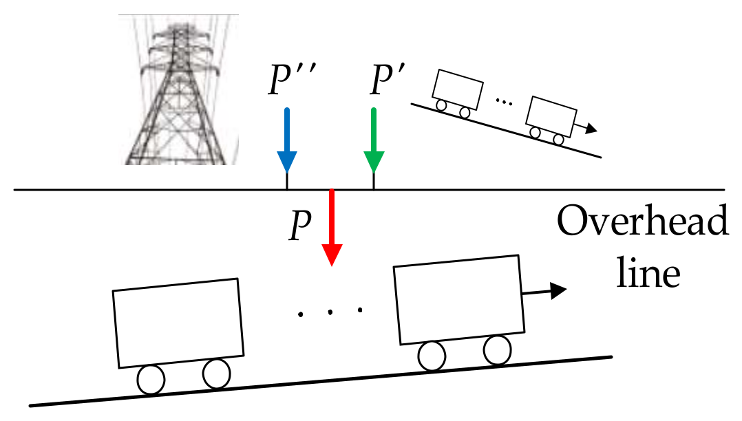
In Figure 5, it is obvious that:
- If P > P′, the consumed power P of the traction trains is partly provided by the grid (P″); the other part comes from the feedback power P′ of the trains running in the reverse direction within the same power supply interval.
- If P ≤ P′, the traction trains do not take power from the grid, and P is entirely provided by P″. If P < P′, the regenerative braking energy cannot be fully utilized.
Combining Figure 4 and Figure 5, whether the regenerative braking energy in a certain power supply interval can be fully utilized needs to be considered for the following:
- The overlapping time Δt of the two types of trains running.
- The total electrical power of all braking train feedback is compared to the total consumed power of all traction trains in Δt.
In this multi-train mode of operation, to establish the total energy consumption model of all trains in the power supply interval (sk, sk+1) for a certain time period, the length of the power supply interval should be considered first, because the complexity of the modeling is different based on the different numbers of trains in one interval.
All the following situations involve the discussion of train operation in the interval (sk, sk+1), assuming that ihjk < 0.
2.7.1. Model with Shorter Supply Intervals
When the length of the power supply section is less than the safe running distance of the train, no more than one train exists on the upper and lower rails in the same power supply section at any time. Consider the six types of possible operation of the train in the time period (ti,k, ti,k+1), as shown in Figure 6a–f. In the figure, the green line represents the running track of the upward train xi, and regenerative braking energy is generated. The red line represents the running track of the downward train yj, which consumes the electrical energy (as below).
In Figure 6a,f, there is no overlapping time between two trains, and the electrical energy fed back by xi will flow to the public grid and cannot be used by yj running in the opposite direction. In other cases, the overlapping time of two trains is
Combining Equations (2)–(5), the traction power consumption P′j,k and the regenerative braking power generationin Ti,j,k are approximately
We denote
Combining with Equations (1), (19), (20) and (22), when the length of the power supply section is less than the safe running distance of the train, the total energy consumption in (ti,k, ti+1,k) is
2.7.2. Model with Longer Supply Intervals
When the length of the power supply interval is greater than the safe running distance of the train, there may be a multitude of trains on the upward and downward tracks in the same power supply interval. The model in this case is relatively complicated. However, considering the influence of the weight, density, and speed of heavy-haul trains on the working voltage of the catenary, the length of the power supply interval generally does not exceed twice the safe running distance of the train. The following discussion is only for the case of a maximum of two trains running under the same power interval in (ti,k, ti+1,k).
The following four events are given according to the time of the incoming and outgoing power supply intervals (sk, sk+1) of the adjacent trains xi−1, xi, and xi+1:
- (1)
- Train xi arrived at sk, train xi−1 left the interval (left the sk+1);
- (2)
- Train xi arrived at sk, train xi−1 did not leave the interval (left the sk+1);
- (3)
- Train xi+1 arrived at sk, train xi did not leave the interval (left the sk+1); and
- (4)
- Train xi+1 arrived at sk, train xi left the interval (left the sk+1),
where (1) and (2) are reciprocal, and (3) and (4) are reciprocal.
Therefore, when t ∈ (ti,k, ti+1,k), there are four possible types of train operation, as summarized in Table 1.
Taking Case 1 as an example, there are 14 possible operations of the upward and downward trains, as shown in Figure 7a–n. The total energy consumption in (ti,k, ti+1,k) is analyzed by considering the energy consumption of the tractor in the up interval (sk+1, sk).
We denote
As shown in Figure 7a, only train xi produces regenerative braking energy and there is no reverse running train in (ti,k, ti+1,k). Therefore, the overlapping time of the upward and downward trains is 0 and the total energy consumption it the interval (sk+1, sk) in (ti,k, ti+1,k) is 0.
As shown in Figure 7b–e, only one train is running on the upward and downward tracks, respectively, in (ti,k, ti+1,k); this situation is analogous to the model in Section 2.7.1. Combining Equations (20)–(24), the total energy consumption of the interval (sk+1, sk) in (ti,k, ti+1,k) is
Figure 7f–n shows the case where two trains are running in the reverse direction during the time (ti,k, ti+1,k). Combining Equations (20) and (24), the total energy consumption of train yj and yj+1 of the interval (sk+1,sk) in (ti,k, ti+1,k) is
In the following analysis, considering the case where the feedback electrical energy of the train xi is used by yj and yj+1, the expression of the total energy consumption of the interval (sk+1, sk) in (ti,k, ti+1,k) is given by combining Equations (1), (20)–(22), (24) and (26).
We denote
- (1)
- Figure 7f,g shows trains yj and yj+1 running simultaneously in (ti,k, τj,k), and only train yj+1 consumes electricity in (τj,k, ). The total energy consumption in the interval (sk+1, sk) in (ti,k, ti+1,k) is
- (2)
- Figure 7h,i,l,m shows that only train yj consumes electricity in (, ), train yj and yj+1 simultaneously run in (, ), and only train yj+1 consumes electricity in (, ). Therefore, the total energy consumption in the interval (sk+1, sk) in (ti,k, ti+1,k) is
- (3)
- Figure 7j shows trains yj and yj+1 running simultaneously in (ti,k, ti+1,k); the total energy consumption in the interval (sk+1, sk) in (ti,k, ti+1,k) is
- (4)
- Figure 7k,n shows that only train yj consumes electricity in (, τj+1,k+1), and trains yj and yj+1 simultaneously run in (τj+1,k+1, ti+1,k). Therefore, the total energy consumption in the interval (sk+1, sk) in (ti,k, ti+1,k) is
Other cases can be analyzed analogously to Case 1, subject to length restrictions, which are not discussed in detail here.
3. Model Verification and Application
The accuracy of the models and the value of the engineering application were verified based on information consisting of the train marshalling, power supply interval, and the line profile provided by Shenshuo Railway, as well as measured velocity and position of the train. Combining Equations (9), (12), (14) and (17), the train energy consumption and regenerative braking energy were calculated and compared with the measured results, as shown in Figure 8. The measured data were obtained through the Shenshuo Railway Security Control Information System (hereafter referred to as the Information System). The system can remotely capture the train operating status information and real-time energy consumption, as recorded by vehicle measurement instruments.
The actual line longitudinal section (part) of Shenshuo Railway is shown in Figure 9, and the added ramp thousandth of some sections in Figure 9 are obtained by Equations (6), as shown in Table 2.
3.1. Energy Consumption and Regenerative Braking Energy Model Verification
According to the hold-out method, additional coefficients in some sections are calculated for two types of trains, as shown in Table 3.
After confirming the additional coefficient, consider the 18,538th train in the upward direction as an example to introduce the calculation method of train energy consumption and regenerative braking energy.
Basic data information:
- Train marshaling: Three HXD1 traction locomotives are followed by 108 C80 trucks.
- The load is 10,800 t and the total mass is 11,400 t.
(1) Xinchengchuan substation to Gushanchuan section post
The length of the interval is 14,535 m, the added ramp thousandth is –9.38, and η2,k is 0.45. The train average speed of 47.3 km/h is assigned to . The instantaneous speed of the train entering this interval is 46 km/h, and the instantaneous speed of departure is 44 km/h (the speed information is collected from the Information System, as below). Based on the above data and Equation (14), it is calculated that the electrical energy fed back by the train in this interval is 1706 kW·h. The Information System collects the feedback power of three traction trains in order of 584 kW·h, 587 kW·h, and 600 kW·h, for a total of 1771 kW·h, as shown in Table 4.
(2) Fugu substation to Gushanchuan section post
The length of the interval is 8509 m, the added ramp thousandth is 11.72, and η1,k is 0.92. The train average speed of 53.3 km/h is assigned to . The instantaneous speed of the train entering this interval is 64 km/h, and the instantaneous speed of departure is 61 km/h. Based on the above data and Equation (12), it is calculated that the active energy of the train in this interval is 1706 kW·h. The Information System collects the feedback power of three traction trains in order of 1235 kW·h, 1247 kW·h, and 926 kW·h, for a total of 3408 kW·h, as shown in Table 4.
At the same time, the above model was also used to calculate the energy consumption and regenerative braking energy of over 85% of Shenshuo Railway from 20 November to 5 December 2017; compared with the measured data of the Information System, the percentage error is generally less than 10%. Owing to limited space, Table 4, Table 5, Table 6 and Table 7 list only the verification results of 20 HXD1 AC trains and 12 SS4B DC trains. Among them, the “calculated value” is the energy consumption or regenerative braking energy calculated from the train data using Equations (9), (12), (14) and (17). The “actual value” is the active or feedback power recorded by the Information System. The “percent error” is used to describe the error between the calculated value and the actual value; active energy is positive, and the feedback power is negative. The upward direction is for the large heavy-haul trains, and the downward direction is for the large empty trains.
Owing to the unavoidable systematic errors such as the line data and locomotive running information involved in the model and the unpredictable accidental errors caused by the difference of weather and driver’s operating modes, the model has higher accuracy and good engineering.
3.2. Energy Analysis of a Single Power Supply Interval
From the analysis in Section 3.1, it can be seen that the accuracy of the train energy consumption and regenerative braking energy model has engineering application value. This section describes how to use the above model and the analysis of Section 2.7 to analyze the overall energy consumption of multiple trains operating in a single power supply interval, considering the available regenerative braking energy. Consider the following two intervals as examples.
(1) Xinchengchuan substation to Gushanchuan section post
Figure 10 shows the train operation diagram in this interval from 12:32:44 to 12:49:44 on 11 December 2017. Train xi and xi+1, 18256 and 18276, respectively, in the upward direction are both towed by the HXD1 locomotive. According to the data collected by the Information System, Δt1 = ti,k − ti+1,k-1 = 372 s and Δt2 = ti+1,k − ti,k = 648 s; and combining Equations (14) and (21), ≈ 6806 kW, = 703.3 kW·h, = 2011.1 kW·h, for a total of 2714.4 kW·h. During the time periods Δt1 and Δt2, the regenerative braking energy generated by the two trains was all sent back to the grid.
(2) Gushanchuan section post to Fugu substation
Figure 11 shows the train operation diagram in this interval from 12:48:27 to 13:03:19 on 11 December 2017. Train xi and xi+1 have the same information as Example (1). The downward train yj (18033) is towed by the SS4B DC locomotive. According to the collected data, Δt1 = ti+1,k − τj,k+1 = 77 s, Δt2 = ti,k+1 − ti+1,k = 306 s, and Δt3 = τj,k − ti,k+1 = 509 s; combining Equations (20) and (21), , , and
are obtained.
In Δt1, considering the regenerative braking energy generated by train xi was used by yj, using Equation (23) or Equation (25), the total energy consumption of the interval is W1 = 14.18 kW·h.
In Δt2, the regenerative braking energy generated by train xi and xi+1 was used by yj; because , all the traction power consumption of the yj traction was provided by xi and xi+1, and the total energy consumption of the interval is W2 = 0.
In Δt3, the regenerative braking energy generated by train xi+1 was used by yj; using Equation (23) or Equation (25), the total energy consumption of the interval is W3 = 103.92 kW·h.
To summarize, the total energy consumption of the intervals in Δt1, Δt2, and Δt3 is W = W1 + W2 + W3 = 118.10 kW·h.
Part of the regenerative braking energy generated by trains xi and xi+1 was used by train yj, and the other part was sent back to the grid in Δt2. By calculation, the regenerative braking energy that is not utilized throughout the entire process is W’ = 419.39 kW·h.
In addition, the total energy consumption of other intervals was also analyzed. Owing to space limitations, it is not elaborated here. From the analysis results, the existing train operation diagram has limited ability to utilize regenerative braking energy. Therefore, without affecting the transport capacity and safety, it is of great significance to study the total train energy consumption by adjusting the operation diagram.
4. Conclusions
From the above analysis, the following conclusions were obtained:
- A model of train energy consumption and regenerative braking energy is proposed based on the single-particle point dynamic model of a train and the theory of railway longitudinal section simplification. The model takes train attributes, line status, and running speed as variables, and the expression is simpler and more convenient than that of multi-particle models. Combined with the current train operation diagram and measured data of Shenshuo Railway, the model has been verified. The results show that the error of the model is generally below 10%. Owing to the complexity of the physical system on which the model relies, and that the influencing factors and error factors are numerous and cannot be completely eliminated, the model can be considered as having good engineering application value.
- Based on the energy consumption and regenerative braking energy model of a single train, the total energy consumption of multiple trains in a single power supply interval is analyzed considering the available regenerative braking energy.
- Subsequent studies may be based on the research results of this study to establish a forecast of the total energy consumption of all trains in the whole section, and to analyze the scheme of the train operation plan that can meet the lowest total energy consumption by adjusting the train operation diagram.
Acknowledgments
This work was supported by Shenhua Group Co., Ltd. science and technology innovation projects (No: CSIE16024877).
Author Contributions
Qiwei Lu and Bangbang He conceived and established model; Bangbang He calculated the relevant results; Qiwei Lu and Mingzhe Wu analyzed the data; Zhichun Zhang, Jiantao Luo, and Yankui Zhang contributed materials; and Bangbang He, Runkai He, and Kunyu Wang wrote the paper.
Conflicts of Interest
The authors declare no conflicts of interest.
References
- Ouyang, H. Study on Control Scheme of High-Power Four-Quadrant Converter. Ph.D. Thesis, Huazhong University of Science and Technology, Wuhan, China, 2012. [Google Scholar]
- Song, K.; Georgios, K.; Li, J.; Wu, M.; Vassilios, G.A. High performance control strategy for single-phase three-level neutral-point-clamped traction four-quadrant converters. IET Power Electron. 2017, 10, 884–893. [Google Scholar]
- Gazafrudi, S.; Langerudy, A.T.; Fuchs, E.; Al-Haddad, K. Power quality issues in railway electrification: A comprehensive perspective. IEEE Trans. Ind. Electron. 2015, 62, 3081–3090. [Google Scholar] [CrossRef]
- He, L.; Xiong, J.; Zhang, P.; Zhang, K. High-performance indirect current control scheme for railway traction four-quadrant converters. IEEE Trans. Ind. Electron. 2014, 61, 6645–6654. [Google Scholar] [CrossRef]
- Steimel, A. Electric railway traction in Europe. IEEE Ind. Appl. Mag. 1996, 2, 6–17. [Google Scholar] [CrossRef]
- Suzuki, T. DC power supply system with inverting substations for traction systems using regenerative brakes. IEE Proc. B Electr. Power Appl. 1982, 129, 18–26. [Google Scholar] [CrossRef]
- Popescu, M.; Bitoleanu, A.; Suru, V.; Preda, A. System for converting the DC traction substations into active substations. In Proceedings of the 9th International Symposium on Advanced Topics in Electrical Engineering (ATEE 2015), Bucharest, Romania, 7–9 May 2015. [Google Scholar]
- Henning, P.H.; Fuchs, H.D.; Le Roux, A.D.; Mouton, H.T. A 1.5-MW seven-cell series-stacked converter as an active power filter and regeneration converter for a DC traction substation. IEEE Trans. Power Electron. 2008, 23, 2230–2236. [Google Scholar] [CrossRef]
- Manno, M.D.; Varilone, P.; Verde, P.; Santis, M.D.; Perna, C.D.; Salemme, M. User friendly smart distributed measurement system for monitoring and assessing the electrical power quality. In Proceedings of the AEIT International Annual Conference (AEIT), Naples, Italy, 14–16 October 2015; pp. 1–5. [Google Scholar]
- Tang, L.; Wu, L. Research on the Integrated Braking Energy Recovery Strategy Based on Supercapacitor Energy Storage. In Proceedings of the International Conference on Smart Grid and Electrical Automation (ICSGEA), Changsha, China, 27–28 May 2017; pp. 175–178. [Google Scholar]
- Moghbeli, H.; Hajisadeghian, H.; Asadi, M. Design and Simulation of Hybrid Electrical Energy Storage (HEES) for Esfahan Urban Railway to Store Regenerative Braking Energy. In Proceedings of the 7th Power Electronics and Drive Systems Technologies Conference (PEDSTC), Tehran, Iran, 16–18 February 2016; pp. 93–98. [Google Scholar]
- Sengor, I.; Kilickiran, H.C.; Akdemir, H.; Kekezoglu, B.; Erdinc, O.; Catalao, J.P.S. Energy management of a smart railway station considering regenerative braking and stochastic behaviour of ESS and PV generation. IEEE Trans. Sustain. Energy 2017, 1–10. [Google Scholar] [CrossRef]
- Kang, X.; Sun, J.; Meng, W. Regulations on Railway Traction Calculation (TB/T1407-201X); National Railway Administration of China: Beijing, China, 2014.
- Xue, Y.; Ma, D.; Wang, L. Calculation Method of Energy Consumption in Train Traction. China Railw. Sci. 2007, 5, 84–86. [Google Scholar]
- Li, Z.; Wei, X.; Wang, H.; Li, J. Optimizing Power for Train Operation Based on ACO. In Proceedings of the 2015 International Conference on Electrical and Information Technologies for Rail Transportation (EITRT), Zhuzhou, China, 17–19 October 2015; pp. 453–462. [Google Scholar]
- Dong, H.R.; Gao, S.; Ning, B.; Li, L. Extended fuzzy logic controller for high speed train. Neural Comp. Appl. 2013, 22, 321–328. [Google Scholar] [CrossRef]
- Zhuan, X.; Xia, X. Speed regulation with measured output feedback in the control of heavy haul trains. Automatica 2008, 44, 242–247. [Google Scholar] [CrossRef]
- Zhu, X.; Xu, Z. Dynamic Simulation of urban rail transit train based on single-particle model. J. China Railw. Soc. 2011, 33, 14–19. [Google Scholar]
- Gao, Z.; Fang, J.; Zhang, Y.; Sun, D.; Jiang, L.; Yang, X. Control Research of Supercapcitor Energy Storage System for Urban Rail Transit Network. In Proceedings of the IEEE International Conference on Information Science and Technology(ICIST), Shenzhen, China, 26–28 April 2014; pp. 181–185. [Google Scholar]
- Saleh, M.; Dutta, O.; Esa, Y.; Mohamed, A. Quantitative analysis of regenerative energy in electric rail traction systems. IEEE Trans. Ind. Appl. 2017, 1–7. [Google Scholar] [CrossRef]
- Adinolfi, A.; Lamedica, R.; Modesto, C.; Prudenzi, A. Experimental assessment of energy saving due to trains regenerative braking in an electrified subway line. IEEE Trans. Power Deliv. 1998, 13, 1536–1542. [Google Scholar] [CrossRef]
- Capasso, A.; Lamedica, R.; Penna, C. Energy regeneration in transportation systems–methodologies for power–networks simulation. IFAC Proc. 1983, 16, 119–124. [Google Scholar] [CrossRef]
- Dominguez, M.; Fernandez-Cardador, A.; Cucala, A.P.; Pecharroman, R.R. Energy Savings in Metropolitan Railway Substations through Regenerative Energy Recovery and Optimal Design of ATO Speed Profiles. IEEE Trans. Autom. Sci. Eng. 2012, 9, 496–504. [Google Scholar] [CrossRef]
- Liu, W.; Li, Q.; Tang, B. Energy saving train control for urban railway train with multi-population genetic algorithm. In Proceedings of the IFITA ‘09. International Forum on Information Technology and Applications, Chengdu, China, 15–17 May 2009; pp. 58–63. [Google Scholar]
- Zhou, Z. Machine Learning; Tsinghua University Press: Beijing, China, 2016; pp. 24–29. [Google Scholar]
- Das Gupta, S.; Pavel, L.; Tobin, K.J. An optimization model to utilize regenerative braking energy in a railway network. In Proceedings of the American Control Conference (ACC), Chicago, IL, USA, 1–3 July 2015; pp. 5919–5924. [Google Scholar]
- Yang, X.; Ning, B.; Li, X.; Tang, T. A two-objective timetable optimization model in subway systems. IEEE Trans. Intell. Transp. Syst. 2014, 15, 1913–1921. [Google Scholar] [CrossRef]
- Liu, J.; Nan, Z. Research on Energy-Saving Operation strategy for multiple trains on the urban subway line. Energies 2017, 10, 2156. [Google Scholar] [CrossRef]
Figure 1.
Schematic diagram of running line.

Figure 2.
Train stress diagram, (a) the uphill traction; (b) the downhill braking.

Figure 3.
Flow of energy consumption and regenerative braking energy.
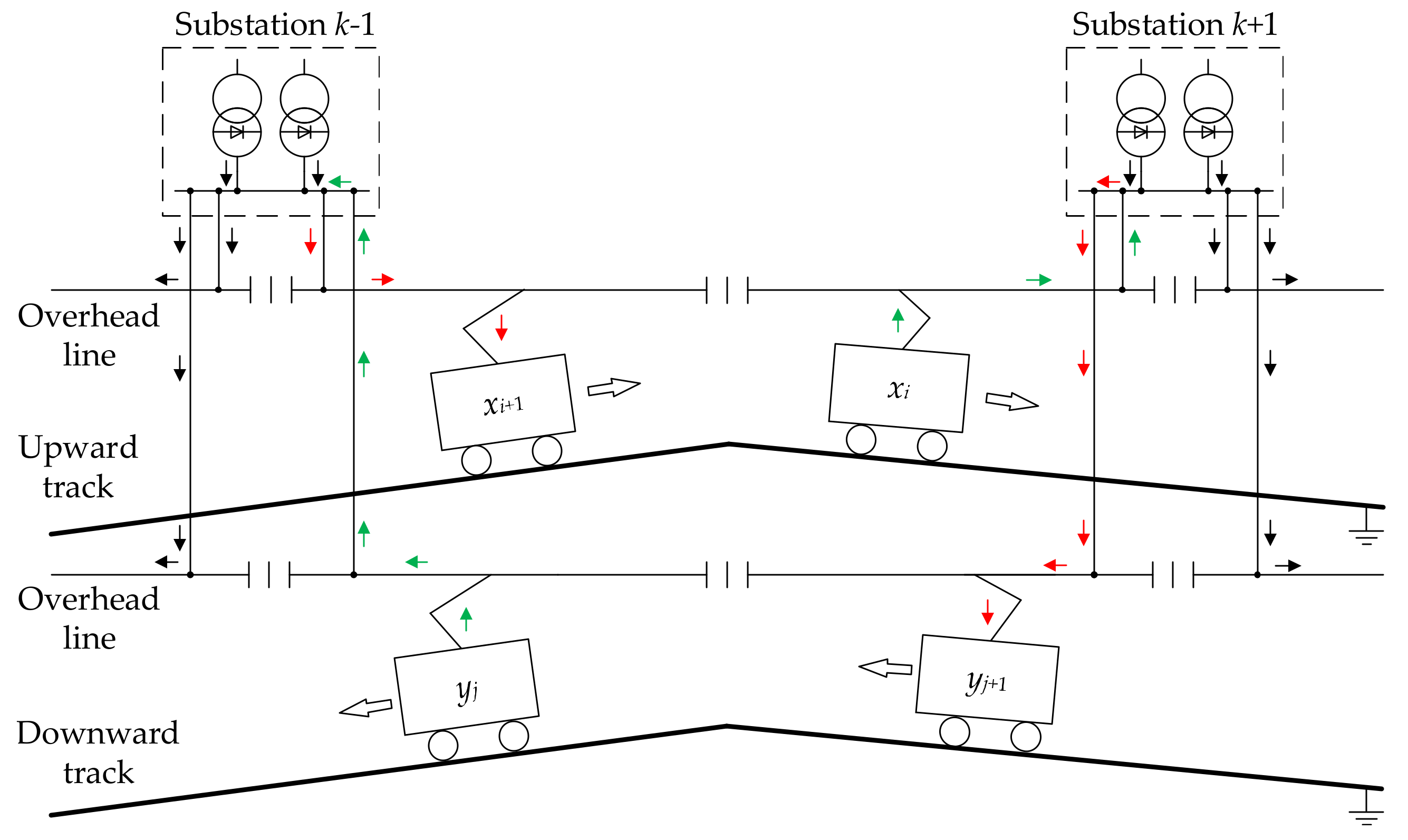
Figure 4.
Power–time distribution of train.

Figure 5.
Power source of traction trains in a certain power supply interval.

Figure 6.
The train diagram of xi and yj in (ti,k, ti,k+1).
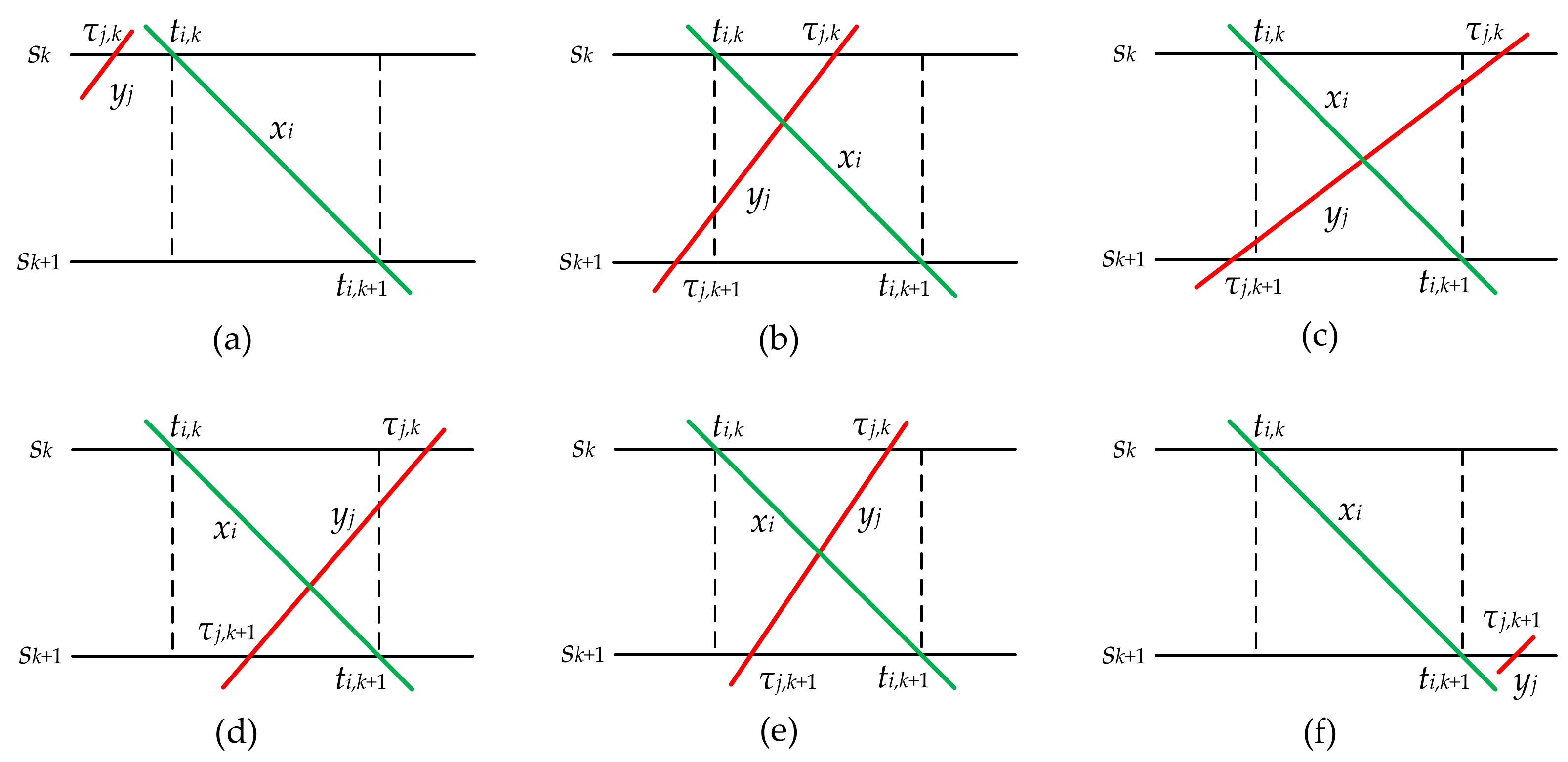
Figure 7.
The train diagram of train xi, xi+1, yj and yj+1 in (ti,k, ti,k+1).
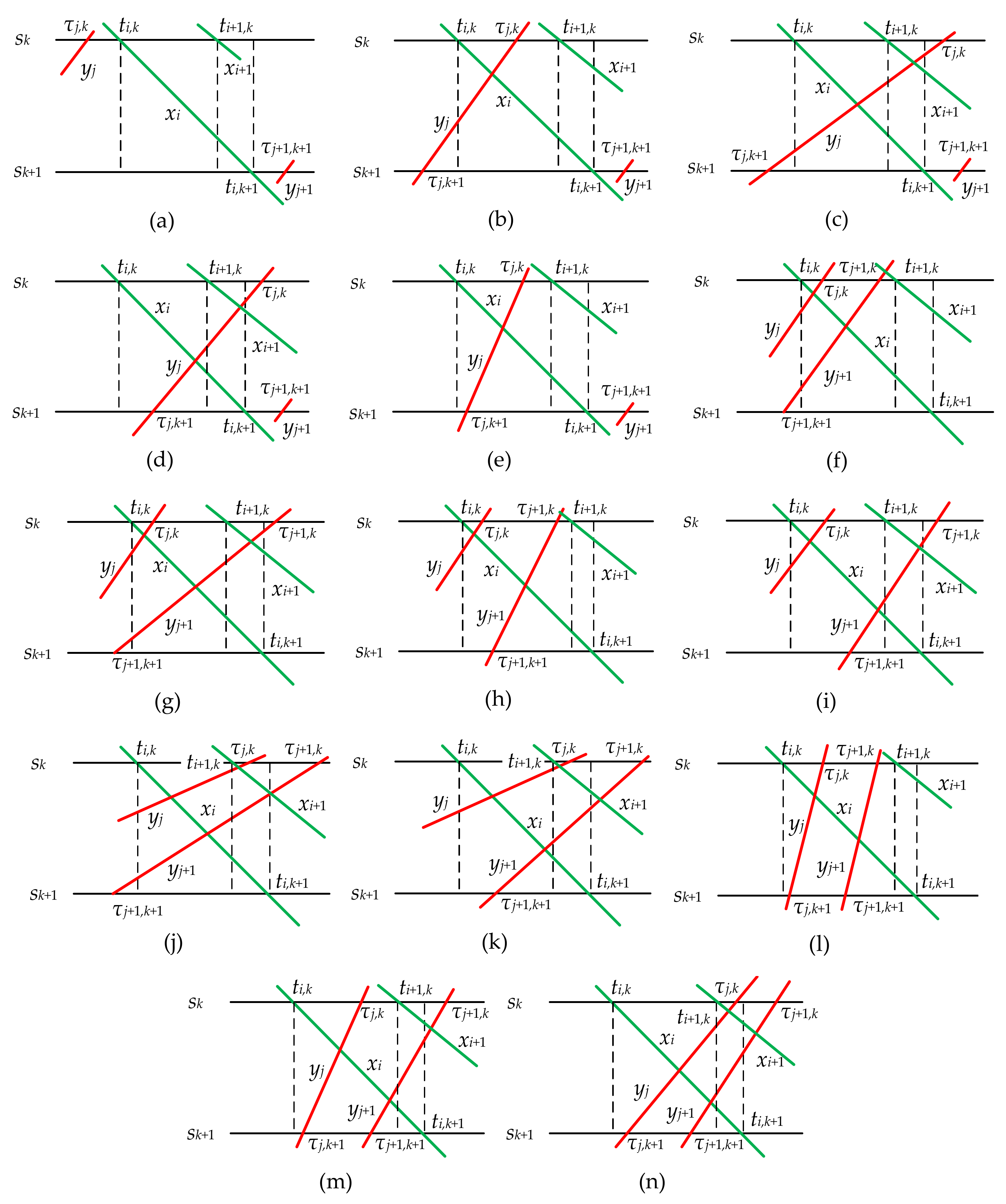
Figure 8.
The flowchart to calculate train energy consumption and regenerative braking.
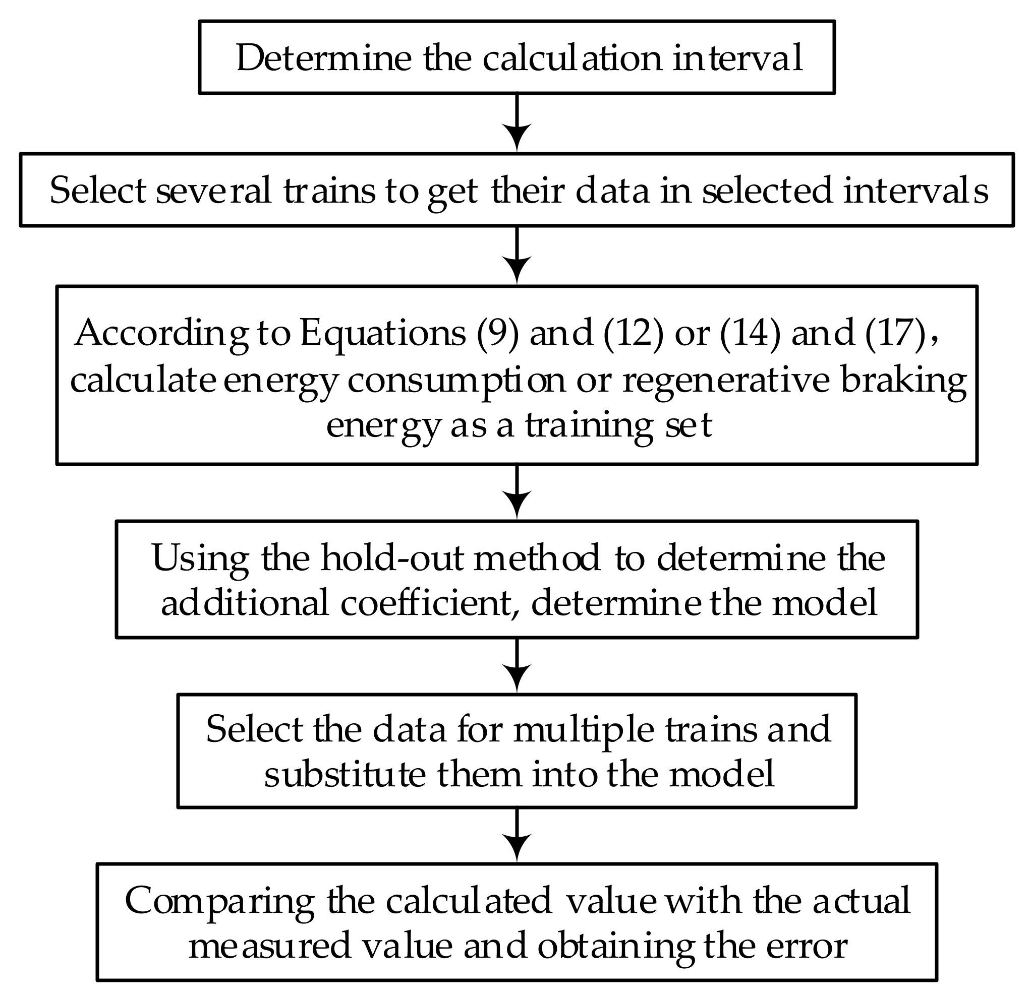
Figure 9.
Shenshuo Railway line longitudinal section (part).

Figure 10.
Section train operation diagram from 12:32:44 to 12:49:44.
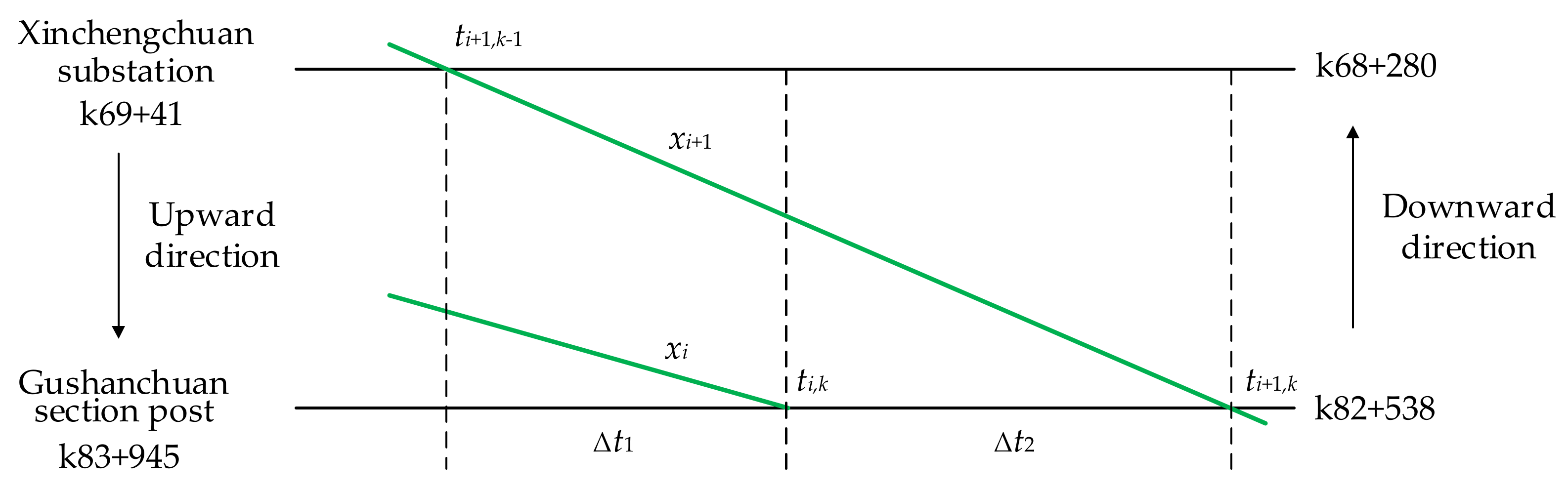
Figure 11.
Section train operation diagram from 12:48:27 to 13:03:19.


Table 1.
Four possible train operation situations.
| Situation | Event Relationship | Mathematical representation | Train Operation |
|---|---|---|---|
| 1 | (1) ∩ (3) | ti−1,k+1 ≤ ti,k and ti+1,k ≤ ti,k+1 | Only train xi runs in (ti,k, ti+1,k) |
| 2 | (1) ∩ (4) | ti−1,k+1 ≤ ti,k and ti+1,k ≥ ti,k+1 | Only train xi run in (ti,k, ti,k+1); no trains run in (ti,k+1, ti+1,k) |
| 3 | (2) ∩ (4) | ti−1,k+1 ≥ ti,k and ti+1,k ≤ ti,k+1 | The train xi−1 and xi run in (ti,k, ti−1,k+1); only train xi run in (ti−1,k+1, ti+1,k) |
| 4 | (2) ∩ (3) | ti−1,k+1 ≥ ti,k and ti+1,k ≥ ti,k+1 | The train xi−1 and xi run in (ti,k, ti−1,k+1); only train xi run in (ti−1,k+1, ti,k+1); no train run in (ti,k+1, ti+1,k) |
As it can accommodate up to two trains running in the running direction of the power supply interval, when train xi runs in the section, whether it runs with the former train xi−1 or the latter train xi+1 at the same time, it is described by the intersection of the two events.
Table 2.
Shenshuo Railway line information (part).
| Category | Power Supply Interval | Length (m) | The Added Ramp Thousandth (‰) |
|---|---|---|---|
| Up direction | Xinchengchuan substation to Gushanchuan section post | 14,535 | –9.38 |
| Gushanchuan section post to Fugu substation | 14,505 | –7.12 | |
| Baode section post to Qiaotou substation | 8059 | 11.72 | |
| Qiaotou substation to Wangjiazhai section post | 13,959 | 8.96 | |
| Wangjiazhai section post to Yinta substation | 12,269 | 6.87 | |
| Down direction | Yinta substation to Wangjiazhai section post | 12,800 | –6.59 |
| Wangjiazhai section post to Qiaotou substation | 14,880 | –8.13 | |
| Qiaotou substation to Baode section post | 8471 | –10.46 | |
| Fugu substation to Gushanchuan section post | 15,879 | 8.29 | |
| Gushanchuan section post to Xinchengchuan substation | 14,258 | 10.29 |
Table 3.
Additional coefficients in some sections.
| Train Type | Power Supply Interval | η1,k | η2,k |
|---|---|---|---|
| HXD1 | Xinchengchuan substation to Gushanchuan section post | 0.77 | 0.45 |
| Gushanchuan section post to Fugu substation | 0.76 | 0.53 | |
| Baode section post to Qiaotou substation | 0.92 | 0.79 | |
| Qiaotou substation to Wangjiazhai section post | 0.91 | 0.59 | |
| Wangjiazhai section post to Yinta substation | 0.89 | 0.52 | |
| SS4B | Yinta substation to Wangjiazhai section post | 0.80 | — |
| Wangjiazhai section post to Qiaotou substation | 0.78 | — | |
| Qiaotou substation to Baode section post | 0.92 | — | |
| Fugu substation to Gushanchuan section post | 0.93 | — | |
| Gushanchuan section post to Xinchengchuan substation | 0.91 | — |
Since the SS4B DC traction locomotive does not produce regenerative braking energy when going downhill, there is no corresponding additional coefficient η2,k.
Table 4.
Verification results of interval energy consumption and regenerative braking energy for upstream AC trains.
Table 4.
Verification results of interval energy consumption and regenerative braking energy for upstream AC trains.
| Train Number | Xinchengchuan Substation to Gushanchuan Section Post | Gushanchuan Section Post to Fugu Substation | Baode Section Post to Qiaotou Substation | Qiaotou Substation to Wangjiazhai Section post | Wangjiazhai Section Post to Yinta Substation | ||||||||||
|---|---|---|---|---|---|---|---|---|---|---|---|---|---|---|---|
| Calculated Value | Actual Value | Percent Error | Calculated Value | Actual Value | Percent Error | Calculated Value | Actual Value | Percent Error | Calculated Value | Actual Value | Percent Error | Calculated Value | Actual Value | Percent Error | |
| 18538 | −1706 | −1771 | 3.65% | −1420 | −1506 | 5.68% | 3612 | 3408 | 5.97% | 4460 | 4696 | 5.02% | 3705 | 3778 | 1.94% |
| 18126 | −1691 | −1525 | 10.87% | −1464 | −1346 | 8.75% | 3595 | 3734 | 3.73% | 4901 | 4826 | 1.56% | 3374 | 3507 | 3.80% |
| 18125 | −1692 | −1709 | 1.01% | −1446 | −1317 | 9.78% | 3681 | 3532 | 4.22% | 4476 | 4666 | 4.07% | 3701 | 3681 | 0.54% |
| 18268 | −1712 | −1718 | 0.33% | −1463 | −1619 | 9.61% | 3685 | 3568 | 3.27% | 4828 | 4661 | 3.59% | 3337 | 3469 | 3.79% |
| 18072 | −1712 | −1669 | 2.60% | −1408 | −1534 | 8.23% | 3664 | 3663 | 0.03% | 4821 | 4768 | 1.12% | 3355 | 3417 | 1.82% |
| 18106 | −1713 | −1622 | 5.62% | −1435 | −1455 | 1.35% | 3525 | 3534 | 0.26% | 4886 | 4886 | 0.01% | 3388 | 3346 | 1.27% |
| 18470 | −1791 | −1791 | 0.01% | −1387 | −1478 | 6.17% | 3504 | 3639 | 3.70% | 4611 | 4538 | 1.61% | 3605 | 3549 | 1.59% |
| 18070 | −1724 | −1832 | 5.90% | −1435 | −1432 | 0.18% | 3707 | 3662 | 1.24% | 4715 | 4840 | 2.58% | 3203 | 3349 | 4.36% |
| 18660 | −1730 | −1662 | 4.08% | −1403 | −1447 | 3.01% | 3611 | 3678 | 1.82% | 4786 | 4438 | 7.83% | 3492 | 3433 | 1.72% |
| 18436 | −1660 | −1625 | 2.16% | −1456 | −1501 | 2.97% | 3613 | 3800 | 4.92% | 4847 | 4636 | 4.55% | 3261 | 3111 | 4.82% |
The traction locomotive’s mass of each train is 600 t, and the total masses of truck and cargo is 10,800 t.
Table 5.
Verification results of interval energy consumption and regenerative braking energy for downstream AC trains.
Table 5.
Verification results of interval energy consumption and regenerative braking energy for downstream AC trains.
| Train Number | Yinta Substation to Wangjiazhai Section Post | Wangjiazhai Section Post to Qiaotou Substation | Qiaotou Substation to Baode Section Post | Fugu Substation to Gushanchuan Section Post | Gushanchuan Section Post to Xinchengchuan Substation | ||||||||||
|---|---|---|---|---|---|---|---|---|---|---|---|---|---|---|---|
| Calculated Value | Actual Value | Percent Error | Calculated Value | Actual Value | Percent Error | Calculated Value | Actual Value | Percent Error | Calculated Value | Actual Value | Percent Error | Calculated Value | Actual Value | Percent Error | |
| 18013 | −258 | −279 | 7.45% | −461 | −457 | 0.88% | −463 | −478 | 3.19% | 1450 | 1473 | 1.54% | 1538 | 1574 | 2.27% |
| 18001 | −252 | −244 | 3.43% | −442 | −410 | 7.85% | −450 | −458 | 1.77% | 1420 | 1457 | 2.52% | 1546 | 1456 | 6.18% |
| 18767 | −257 | −249 | 3.06% | −452 | −468 | 3.45% | −468 | −498 | 6.07% | 1483 | 1493 | 0.70% | 1521 | 1518 | 0.21% |
| 17051 | −315 | −312 | 0.97% | −549 | −575 | 4.50% | −552 | −587 | 5.99% | 1712 | 1589 | 7.73% | 1882 | 1834 | 2.60% |
| 16537 | −354 | −381 | 6.96% | −621 | −602 | 3.13% | −649 | −617 | 5.18% | 1980 | 1886 | 4.96% | 2050 | 1941 | 5.62% |
| 17043 | −318 | −352 | 9.76% | −578 | −633 | 8.61% | −508 | −529 | 4.05% | 1718 | 1739 | 1.19% | 1844 | 1757 | 4.92% |
| 16587 | −358 | −362 | 0.97% | −611 | −652 | 6.22% | −611 | −582 | 4.99% | 2028 | 1910 | 6.20% | 2099 | 1954 | 7.42% |
| 18031 | −266 | −261 | 1.96% | −463 | −491 | 5.71% | −465 | −433 | 7.38% | 1517 | 1673 | 9.31% | 1589 | 1731 | 8.21% |
| 18109 | −271 | −277 | 2.29% | −451 | −478 | 5.60% | −464 | −443 | 4.67% | 1454 | 1431 | 1.63% | 1571 | 1565 | 0.41% |
| 18241 | −262 | −253 | 3.59% | −465 | −472 | 1.54% | −484 | −498 | 2.84% | 1527 | 1645 | 7.20% | 1588 | 1654 | 3.99% |
The traction locomotive’s mass of each train is 600 t, and the total masses of truck and cargo are, respectively, 2160 t, 2040 t, 2160 t, 2668 t, 3036 t, 2622 t, 3036 t, 2160 t, 2120 t, and 2160 t.
Table 6.
Verification results of energy consumption of DC trains in the uphill section.
| Train Number | Baode Section Post to Qiaotou Substation | Qiaotou Substation to Wangjiazhai Section Post | Wangjiazhai Section Post to Yinta Substation | ||||||
|---|---|---|---|---|---|---|---|---|---|
| Calculated Value | Actual Value | Percent Error | Calculated Value | Actual Value | Percent Error | Calculated Value | Actual Value | Percent Error | |
| 18446 | 3699 | 3427 | 7.95% | 4852 | 4491 | 8.04% | 3361 | 3133 | 7.28% |
| 18534 | 3733 | 3841 | 2.80% | 4826 | 4444 | 8.60% | 3430 | 3255 | 5.37% |
| 18360 | 3693 | 3744 | 1.36% | 4418 | 4673 | 5.46% | 3334 | 3385 | 1.49% |
| 17012 | 3681 | 3827 | 3.81% | 4604 | 4862 | 5.32% | 3301 | 3477 | 5.07% |
| 18494 | 3799 | 4133 | 8.08% | 4571 | 4937 | 7.42% | 3433 | 3575 | 3.97% |
| 18006 | 3733 | 3517 | 6.13% | 4613 | 4793 | 3.75% | 3632 | 3952 | 8.10% |
The traction locomotive’s mass of each train is 736 t, and the total masses of truck and cargo are, respectively, 10,800 t, 10,800 t, 10,184 t, 10,416 t, 10,600 t, and 10,800 t.
Table 7.
Verification results of energy consumption of DC trains in the downhill section.
| Train Number | Fugu Substation to Gushanchuan Section Post | Gushanchuan Section Post to Xinchengchuan Substation | ||||
|---|---|---|---|---|---|---|
| Calculated Value | Actual Value | Percent Error | Calculated Value | Actual Value | Percent Error | |
| 18439 | 1562 | 1526 | 2.37% | 1647 | 1693 | 2.74% |
| 17139 | 1647 | 1623 | 1.50% | 1543 | 1573 | 1.93% |
| 18367 | 1552 | 1603 | 3.17% | 1611 | 1591 | 1.28% |
| 18101 | 1511 | 1510 | 0.04% | 1641 | 1553 | 5.67% |
| 18757 | 1631 | 1585 | 2.88% | 1588 | 1676 | 5.24% |
| 18753 | 1635 | 1650 | 0.93% | 1633 | 1686 | 3.14% |
The traction locomotive’s mass of each train is 736 t, and the total masses of truck and cargo are, respectively, 2160 t, 2160 t, 2160 t, 2080 t, 2160 t, and 2160 t.
© 2018 by the authors. Licensee MDPI, Basel, Switzerland. This article is an open access article distributed under the terms and conditions of the Creative Commons Attribution (CC BY) license (http://creativecommons.org/licenses/by/4.0/).
Share and Cite
MDPI and ACS Style
Lu, Q.; He, B.; Wu, M.; Zhang, Z.; Luo, J.; Zhang, Y.; He, R.; Wang, K. Establishment and Analysis of Energy Consumption Model of Heavy-Haul Train on Large Long Slope. Energies 2018, 11, 965. https://doi.org/10.3390/en11040965
AMA Style
Lu Q, He B, Wu M, Zhang Z, Luo J, Zhang Y, He R, Wang K. Establishment and Analysis of Energy Consumption Model of Heavy-Haul Train on Large Long Slope. Energies. 2018; 11(4):965. https://doi.org/10.3390/en11040965
Chicago/Turabian StyleLu, Qiwei, Bangbang He, Mingzhe Wu, Zhichun Zhang, Jiantao Luo, Yankui Zhang, Runkai He, and Kunyu Wang. 2018. "Establishment and Analysis of Energy Consumption Model of Heavy-Haul Train on Large Long Slope" Energies 11, no. 4: 965. https://doi.org/10.3390/en11040965
Note that from the first issue of 2016, this journal uses article numbers instead of page numbers. See further details here.