Article

A Biophysical Perspective of IPCC Integrated Energy Modelling

Australian-German College of Energy and Climate, The University of Melbourne, Melbourne 3010, Australia
Energies 2018, 11(4), 839; https://doi.org/10.3390/en11040839
Submission received: 5 February 2018 / Revised: 19 March 2018 / Accepted: 2 April 2018 / Published: 4 April 2018
(This article belongs to the Section A: Sustainable Energy)

Abstract

:
The following article conducts an analysis of the Intergovernmental Panel on Climate Change (IPCC) Fifth Assessment Report (AR5), specifically in relation to Integrated Assessment Models (IAMs). We focus on the key drivers of economic growth, how these are derived and whether IAMs properly reflect the underlying biophysical systems. Since baseline IAM scenarios project a three- to eight-fold increase in gross domestic product (GDP)-per-capita by 2100, but with consumption losses of only between 3–11%, strong mitigation seems compatible with economic growth. However, since long-term productivity and economic growth are uncertain, they are included as exogenous parameters in IAM scenarios. The biophysical economics perspective is that GDP and productivity growth are in fact emergent parameters from the economic-biophysical system. If future energy systems were to possess worse biophysical performance characteristics, we would expect lower productivity and economic growth, and therefore, the price of reaching emission targets may be significantly costlier than projected. Here, we show that IAMs insufficiently describe the energy-economy nexus and propose that those key parameters are integrated as feedbacks with the use of environmentally-extended input-output analysis (EEIOA). Further work is required to build a framework that can supplement and support IAM analysis to improve biophysical rigour.

1. Introduction

1.1. Scenario Modelling

Much of the Intergovernmental Panel on Climate Change (IPCC) Work Group 3 (Mitigation) reporting relies on prospective energy modelling based on Integrated Assessment Models (IAMs) [1]. Baseline scenarios assume a three- to eight-fold increase in gross domestic product (GDP)-per-capita by 2100 ([1], p. 426). GDP growth is composed of GDP per-capita and population growth and connected to emissions with the Kaya identity, which underlies the emissions scenario literature ([2], p. 105). The Kaya identity states that total CO 2 emissions are the product of population, GDP per-capita, energy intensity and carbon intensity, shown in Equation (1).
CO 2 Emissions = Population × GDP Population × Energy GDP × CO 2 Energy
Since strong mitigation scenarios result in global consumption (in this context, consumption refers to economic goods and services) losses in 2100 of only between 3–11% relative to the baseline ([1], p. 419), strong mitigation seems consistent with economic growth. In the IPCC Fifth Assessment Report (AR5), consumption losses are based on incremental costs relative to a baseline ([3], p. 1221) and do not take into account co-benefits or the adverse side-effects of mitigation actions ([4], p. 1292).
However, as Stern [5] notes, with assumed growth of over 1% over a century and with modest damages, the nature of compound growth ensures that ‘future generations are assumed to be much better off’. When the assumption of growth is relaxed, the cost of mitigation, as reflected in the social cost of carbon (SCC), can increase by orders of magnitude [6]. The challenges of the long time frames of interest in climate mitigation are reflected in the wide divergence in SCC estimates that result from different assumptions in parameters such as the discount rate and ‘pure rate of time preference’ (e.g., Smith [7], Pindyck [8]).
Since there are no economic-development scenarios available in the literature that extend to the long-term time horizons required for climate scenarios, GDP growth and total factor productivity are exogenous inputs. However, the biophysical economics (biophysical economics (BPE) is defined as ‘the study of the ways and means by which human societies procure and use energy and other biological and physical resources to produce, distribute, consume and exchange goods and services, while generating various types of waste and environmental impacts’ [9]. ‘Biophysical’ refers to the material world and can be contrasted with an anthropocentric perspective, of which mainstream economics is a subset ([10], p. 1)) perspective is that these are in fact emergent parameters from the economic-biophysical system.
Furthermore, the assumption that future energy systems will possess equivalent or superior biophysical and economic qualities is contested within the biophysical literature [11,12,13]. If future energy systems were to possess worse biophysical performance characteristics, productivity and economic growth may be overstated in the IAM literature, and therefore, the price of reaching emission targets may be significantly costlier than projected.
Section 1.2 defines and describes biophysical economics. Section 2 briefly describes integrated assessment models. Section 3 explores assumptions in the modelling, with an emphasis on a biophysical perspective. Section 4 identifies two approaches to connecting conventional economic approaches with a biophysical perspective. Section 4.1 introduces a preliminary framework for supporting and supplementing integrated models, and finally, Section 5 provides some overarching conclusions.

1.2. Biophysical Economics

Biophysical economics (BPE) is related to the field of industrial ecology, which uses the tools of life-cycle assessment (LCA) and environmentally-extended input-output analysis (EEIOA) to explore the full environmental assessment of the life cycle of products and services. The focus of BPE is the energy-environment-economic nexus.
Net energy analysis (NEA) refers to a class of methods that are physically based, which are used to determine the efficiency or productivity of energy supply technologies [14]. Results are presented in the form of energy return ratios (ERR), of which EROI is the most commonly used (see Equation (2)). EROI is a unitless ratio, defined as the ratio of the gross flow of energy E g over the lifetime of the project, and the sum of the energy for construction E c , operation E o p and decommissioning E d ([15] Equation (1)). The energy inputs include both the direct and indirect energy. Murphy et al. [16] state that ‘EROI is the ratio of how much energy is gained from an energy production process compared to how much of that energy (or its equivalent from some other source) is required to extract, grow, etc., a new unit of the energy in question’.
E R O I = E g E c + E o p + E d
The ratio provides an energetic valuation of the fuel, which may, or may not, correlate with the conventional economic valuation. An energetic valuation of fuels and electricity, based on EROI, conveys information on the potential benefit of using that energy source that may not be obvious from the price system alone.
There may be overlap between energetic and economic valuations, determined, in part, by the capital and energy intensity of the energy supply system [17]. For example, the cost of oil and gas production has been shown to be inversely related to EROI [18,19], but the market price is overlaid with cycles and subject to many factors [20]. On the other hand, the price of solar photovoltaics may be a poor proxy for its energetic evaluation [21]. Nuclear power is subject to economic, regulatory and social constraints (e.g., von Hippel et al. [22]), rather than underlying biophysical constraints, depending on factors such as reactor type, ore grade and enrichment method [23].
Ideally, EROI should provide a means to supplement conventional economic and environmental analysis and inform and shape energy transition analysis. However, a lack of methodological consistency has led to contestation of NEA’s relevance to the broader and IAM scenario literature [21].

2. Integrated Assessment Models

Stabilizing greenhouse gas emissions will require transformation of energy supply and energy end-use services ([1], p. 420). Net global CO 2 energy supply emissions must eventually be brought to, or below, zero. The main IPCC modelling tool for assessing transformation pathways are IAMs ([1], p. 420). IAMs employ a simplified and stylised approach to physical and social systems, but integrate energy, the carbon cycle and economic systems. They typically incorporate all of the major energy sources (i.e., coal, oil, gas, nuclear, renewables), but may constrain specific sources, such as nuclear, or coal with carbon capture.
A key use of IAMs has been to produce energy scenarios for representative concentration pathways (RCPs) as part of the IPCC climate mitigation process. AR5 defined seven CO2eq concentration categories (see Clarke et al. [1], Table 6.2) and selected four that corresponded with RCP pathways: RCP2.6, 4.5, 6.0 and 8.5. The RCP scenarios are considered to be plausible and illustrative, but do not have probabilities attached to them [24]. In AR5, the RCPs superseded the Special Report on Emission Scenarios (SRES) ‘storylines’. The storylines permit harmonisation across models, and are defined as the A1, A2, B1 and B2 scenario families ([2] Box SPM-1). GDP growth is one of several ‘driving forces’, with the A1 storyline adopting the highest economic growth, followed by B1, then A2 and B2. A total of 1184 scenarios was reviewed for AR5 [25], of which a quarter were baseline and three-quarters were mitigation scenarios ([26], p. 9).
Other economic explorations of mitigation measures include energy supply cost curves, marginal abatement cost (MAC) curves (e.g., McKinsey) and cost-benefit studies (e.g., Tol [27], Nordhaus and Boyer [28]). However, AR5 has adopted integrated modelling as the preferred approach due to its high structural detail ([29], p. 534).
Although modelling approaches and objectives differ, all models use economics as the basis for decision making by minimizing the aggregate economic costs of achieving mitigation outcomes ([1], p. 422; [30]). The BPE perspective is that an economic valuation of fuels and electricity may not convey complete information about the potential benefit, or costs, of that energy source. This study is not intended as a systematic review of the IAM scenario database, but a contribution to supplementing and supporting the economic valuation perspective of IAMs with a biophysical energetic valuation perspective.

3. Detailed Exploration of Assumptions

3.1. Total Factor Productivity and GDP Growth

In economic texts (e.g., (Mankiw [31], pp. 249–250), three sources of economic growth are identified: changes in the amount of capital, changes in the amount of labour and changes in total factor productivity (TFP). Since TFP is not directly observable, it is measured indirectly as a residual, or as the growth that remains after accounting for changes in capital and labour.
The concept of TFP can be traced to Robert Solow’s discovery that output rose faster than capital and labour inputs in U.S. time-series data for the period 1909–1949. He appended A t , calling it ‘technical change’, to describe what appeared to be a shift in the production function (see Equation (3)). He explained that the term was meant in the broadest sense, including ‘slowdowns, speed-ups, improvements in the education of the labour force’ and ‘other things’ [32]. It was only later that it was to become a stylized fact that ‘technical change’ (Solow later noted that ‘technical change’ was simply ‘a measure of our ignorance’, which has since been variously termed ‘Solow’s residual’ [33], ‘manna from heaven’ [34], the ‘dark matter of growth’ [35] and most commonly ‘total factor productivity’ in mainstream economics texts [31]) was the primary contribution to national economic growth. In contemporary use, the expression describes a broad range of factors, including technology, education and the role of institutions. The importance of A t is that productivity is the main driver of per-capita growth and a rise in the standard of living [36].
Y t = A t L α K 1 α
where Y, L and K are output, labour and capital. respectively, and α is labour’s factor share.
Beginning with Romer [37], many variants of ‘endogenous growth theory’ were developed that sought to explain and disaggregate A t . Endogenous theory holds that the primary drivers of ‘technological progress’ are human capital, innovation and knowledge, and therefore investment in education, research and development and knowledge production contribute spillovers and positive externalities. The essential feature of endogenous growth theory is the primacy of knowledge capital. For example, Buonanno et al. [38] (Equation (1)) augment the Solow equation with knowledge capital (see Equation (4)).
Y t = A t K R β L α K 1 α
where K R is knowledge capital and β is output elasticity of knowledge capital.
Although there are many approaches for accounting for endogenous technological change [39], nearly all energy-economic models take productivity growth as exogenous and assume average global TFP growth of ∼2–3% per year ([40], Section 3.1). Since there are no economic development scenarios available in the literature that extend to the long-term time horizons required for climate scenarios, GDP growth and total factor productivity are exogenous in the IAM literature. In AR5, all models assume increasing per capita income ([1], p. 426). Income growth is modelled as an exogenous improvement based on productivity growth during the Twentieth Century. The average baseline per-capita growth rate for OECD countries is mostly clustered between 1.2 and 2.0%, while for non-OECD, 3–4% ([1], Figure 6.2). On average, baseline scenarios assume a three- to eight-fold increase in global GDP-per-capita by 2100 ([1], Figure 6.1b). However, recent data on per-capita growth show a marked decline for wealthier nations ([41], Figure 2.6), with attention turning to what has been termed ‘secular stagnation’ and falling productivity growth (e.g., [42,43,44]).
‘Technical change’ also contributes to improved energy efficiency and therefore a decline in energy intensity, discussed in Section 3.2; and a reduction in the cost of energy supply technologies [40,45]. In the IAM literature, ‘endogenous technological change’ is sometimes applied to energy supply, resource availability and end-use technologies through the use of learning curves. Examples include MESSAGE-MACRO [46] and DEN21+ [47]. In modelling, induced technological change tends to reduce the costs of environmental policy and accelerates the learning rates of low-emission energy supply technologies [48].
Whereas neoclassical economics adopts capital and labour as the primary factors of production, with ‘technical change’ or ‘knowledge capital’ driving TFP growth, BPE also adopts energy as a primary factor (e.g., Ayres [49], pp. 385–389). Energy-matter is the principle factor that cannot be physically produced from within the economic system. With respect to energy, civilisation is like any other physical process; that is, as an open, non-equilibrium thermodynamic system that sustains itself with the use and dissipation of energy [50]. The simplest energy-augmented production function, given as indexed parameters, from Lindenberger and Kümmel [51] is given as:
Y = y 0 K α L β E 1 α β
where Y, y 0 , L, K and E are output, output at time zero, labour, capital and energy, respectively, and α and β are capital and labour’s factor share, respectively.
Whereas neoclassical economics assumes that there is, in principle, no limit to the substitution of energy, the BPE perspective is that there is a lower bound to substitution. Kumhof and Muir [52] term this lower bound the ‘entropy boundary’, alluding to the second law of thermodynamics. Kümmel et al. [53], Kümmel [54], Giraud and Kahraman [55], Keen and Ayres [56] and Ayres and Warr [33] have modelled variations on the neoclassical Cobb–Douglas aggregate production function and found that the inclusion of energy accounts for around half to two-thirds of the observed economic growth that is usually attributed to TFP. This implies that the output elasticity, with respect to energy, is much greater than its factor share.
IAMs generally include energy as a factor of production, but implicitly set the output elasticity as equal to the factor share, which is typically less than 10% in the developed economies (e.g., Edenhofer et al. [45], Equation (1)). If the BPE hypothesis is correct, it would require that the A t term (Scientific equations usually include dimensions for dimensional analysis. However, economic modelling of production functions of this type usually apply dimensionless indexes. Barnett [57] argued that the use of dimensions may be either meaningless or economically unreasonable. In this case, the A t term is dimensionless.) be endogenous and a key feedback loop in IAMs.

3.2. Declining Energy Intensity

A declining energy intensity permits higher economic growth for a given greenhouse gas (GHG) emission budget. The historical trend is towards declining energy intensity since GDP growth is generally greater than energy use growth. The reduction in energy intensity for AR5 baseline scenarios is ∼61–80% up to 2100 ([1], Figure 6.17), equating to an averaged ∼−1.0–−1.8%/year. However, the historical change in global energy intensity over the period 1970–2010 averaged −0.8%/year ([1], Figure 6.1c). EIA [58] shows a return to trend decline since a plateau around 2010 (Different primary energy conventions across energy reporting agencies [59] and differences in GDP measurement result in differences in reported changes in energy intensity. For example, EIA [58] shows greater decline than Clarke et al. [1]. EIA [60] (Table J3) adopt $PPP, while Clarke et al. [1] (Figure 6.1) adopt market exchange rates. This study relied on Clarke et al. [1] to ensure like-for-like comparisons.).
IAMs are, on average, modelling a baseline reduction in energy intensity of 25–125% greater than the average for the period 1970–2010 [13,61]. Some of the bottom-up optimisation models cited in the AR5 project even greater decoupling: Teske [62] assume −3.4%/year and Jacobson and Delucchi [63] assume −3.6%/year. Clarke et al. [1] (Figure 6.2) shows 11 OECD baseline projected projections for 2010–2050 at higher than ∼−2.0%/year and 11 non-OECD at higher than ∼−3.0%/year. The 530–580-ppm and 430–480-ppm CO 2 -eq scenarios project an additional reduction over the baseline of ∼18–45% for the period up to 2100.
In a review of the AR5 430-530 ppm scenarios, the additional annual investment for efficiency far exceeded the additional investment in energy supply ([3], Figure 16.3). However, models do not endogenize the increased embodied energy of the technical efficiency measures of vehicles, buildings and energy-consuming equipment. IAMs account for costs in the construction stage, but are implicitly assuming that the energy intensity of manufacturing, construction and energy consuming equipment is the economy-wide average. Since service sectors are both less energy intensive and comprise a significant share of developed economies, the economy-wide intensity is typically less than for manufacturing and construction (e.g., Hertwich and Peters [64]). In some cases, the improved efficiency during the use stage (The ‘use stage’ is one of several stages in life-cycle assessment. Other stages include raw material extraction, processing, manufacturing or production, use and maintenance and end-of-life [65]) is significantly offset by the additional embodied energy during the production stage. Examples include electric vehicles [66] and housing that conforms to the Passive House Standard [67]. Since energy efficiency protocols almost universally apply only to energy used during the use stage, the problem can arise of ‘overshooting’ the optimal lifetime efficiency.
Projections of energy intensity are partly based on historical energy efficiency improvements. However, it can be difficult to model the human behavioural and income effects resulting from Jevon’s paradox [68]. The direct rebound effect posits that efficiency lowers the cost of an energy service, leading to increased use of that service, termed the income effect [69]. However, the indirect, economy-wide and transformational effects are significant and pervasive in producer economies such as China [70]. On the one hand, the technical efficiency gains of delivering end-use energy services are very large [71], but translating technical gains into sustained reductions has proven allusive absent sustained rises in energy prices [72]. AR5 identified the efficiency rebound effect in Bruckner et al. [29] (Section 7.12.1), Kolstad et al. [73] (Section 3.9.5) and Blanco et al. [74] (Section 5.6.2); however, the adoption of exogenous energy intensity as part of the scenario ‘storylines’ essentially invalidates any macro integration of rebound.

3.3. Life-Cycle Assessment Methodologies

The IPCC Special Report ‘Renewable Energy Sources and Climate Change Mitigation’ contained a chapter [75] on sustainable development, which included a broad discussion of life-cycle analysis (LCA) and net-energy. The report identified the limitations of attributional, process-based life cycle assessments (LCAs) ([75], p. 730) and the need to identify uncertainties, but nonetheless, used an attributional approach to present the main results. Since non-fossil technologies are generally more capital intensive, the importance of indirect energy, and therefore a comprehensive LCA, will likely increase in the future [76].
The two main issues are, firstly, process-based analysis results in a truncated boundary and therefore understates the indirect embodied energy [77]. In LCAs, there is is no requirement to ensure that an analysis meets a prescribed level of ‘completeness’. ISO [78] (Section 6.4.5) and ISO [79] (Section 5.2.3) require that stages, unit processes or inputs are followed until they ‘lack significance’ within the given scope. This can be problematic when LCAs are applied to energy transition exercises since a high level of ‘completeness’ is often assumed by modellers applying LCA data [21]. Environmentally-extended input-output analysis (EEIOA) connects energy flows to monetary flows using national input-output (I/O) tables and ensures systematic completeness. However, the assumption of heterogeneity introduces aggregation error. The respective benefits of process and I/O analysis can be combined with hybrid-LCA [65].
Secondly, an attributional approach considers the embodied energy of the technology in question, but does not consider the broader impacts that might result from the decision to adopt or install a specific technology ([75], p. 730). In contrast, a consequential approach considers the broader impacts. However, it can be methodologically difficult to evaluate consequential changes to energy systems with LCA approaches (e.g., Jones et al. [80]). Consequential analyses are generally more comprehensive, but also carry greater uncertainty and the risk of double counting due to overlap between studies. The paucity of energy technology consequential studies reflects this, and Sathaye et al. [75] (p. 730) note that the limited number of studies precludes the incorporation of consequential analysis into IAMs. Other factors that limit the use of LCAs in integrated modelling include substantial variability in published LCA results and differences in the LCA technique ([75], p. 730). Some IAMs adopt a simplified approach to consequential changes related to variable renewable energy. For example, WITCH and MESSAGE adopt flexibility and capacity constraints that weight the dispatchability of different generator types [81].
The LCA literature emphasises the use of standard guidelines and the primacy of datasets based on ‘complete and verifiable documentation’ [82]. The limitation of standard guidelines is that studies are then restricted to answering the research questions to which that methodology is suited. In the context of electricity system transitions, considerations relating to the engineering-systems perspective of electricity supply are generally treated as lying outside the domain of conventional life-cycle research.
In the case of solar photovoltaics for instance, the choice of goal definition, methodology and boundaries can alter the EROI by an order of magnitude [21]. Since the LCA literature has tended to converge towards a standard suite of guidelines, study results emphasise differences between studies, rather than a high level of completeness. The use of attributional, process-based LCAs may be unsuited to the task of assessing large-scale energy transitions, unless they are combined with some form of consequential approach.

3.4. Steel and Cement

IAMs mostly ignore material cycles and recycling [83], although some material flows are considered. In the AR5 literature, life-cycle analysis is identified (e.g., Sathaye et al. [75], p. 730) but is not broadly adopted in IAMs. Similarly, material scarcity associated with low-emission energy sources is identified ([29], p. 549), but not explicitly modelled in IAMs.
Some IAMs include material flows that have a significant emissions footprint, such as steel and cement; these comprise 28% and 27% of direct industrial CO 2 emissions, respectively ([84], Figure 2.22). However, no IAMs fully integrate material flows into the physical system [83]. For example, IMAGE is one of the most comprehensive models for the steel cycle and its emissions, but steel demand is modelled as a function of per-capita GDP ([85], Figure 1). A more detailed approach would have been to link steel production to the main steel consuming sub-sectors: buildings and transportation ([83] p. 17).
Furthermore, the embodied material and energy of energy supply technologies are not modelled. Fossil fuel-derived electricity is significantly more lifecycle greenhouse intensive than renewable sources due to direct combustion ([29], Figure 7.6); [86]. On the other hand, renewable and nuclear electricity possess a higher embodied material and energy content [86,87]. Wind, ocean and CSP require more steel and cement than fossil fuel plants, per unit of electricity generated ([29], p. 549).

3.5. Biofuels

AR5 devoted a chapter to bioenergy ([88], Chapter 11), which covered life-cycle emissions of biofuels. The life-cycle emissions are a proxy for embodied energy, but land use changes significantly increase life-cycle emissions relative to embodied energy ([88], Figure 11.24). Most of the biofuel-related LCA literature applies carbon accounting rather than energy accounting, but arrives at similar conclusions to Hall et al. [89]; for example, DeCicco et al. [90] found that U.S. corn biofuel only offsets CO 2 emissions by around a third of that required to achieve carbon neutrality. Much of the studied bioenergy is marginal from a net-energy perspective ([91], Figure 2), ([92], Figure 8), but some production systems (e.g., Brazilian ethanol) may be favourable in some contexts [93].
Virtually all bottom-up energy scenario models that include biofuels adopt gross energy flows (e.g., Elliston et al. [94]). In IAMs, projected costs are modelled, but implicitly assume that the energy intensity of energy supply technologies is commensurate with incumbent sources. Where the EROI of a biofuel production system is significantly less than conventional fuels, the net-energy may be much less than assumed, thereby overstating the extent of fuel substitution.
The use of biomass energy with carbon dioxide capture and storage (BECCS), will reduce the EROI further since CCS is estimated to consume 25–35% of gross output ([95], p. 338). In a review of IAMs, Bruckner et al. [29] (p. 559) found that a carbon price of USD 100 per tonne CO2eq would be sufficient to drive large-scale deployment of BECCS. Yet, from a biophysical perspective, energy sources with an EROI in the range of 0.8–3:1 cannot support an advanced society [12], irrespective of carbon price. AR5 identifies several limiting factors for BECCS, including land availability, a sustainable supply of biomass and storage capacity ([1], p. 485), but does not identify EROI or net-energy as a constraint.

3.6. EROI Constraints

The theoretical global potential of RE sources is substantially higher than global energy demand ([96], p. 10). Studies have typically focused on economic costs, land availability and kinetic or radiative energy constraints. However, AR5 identified the issue of whether some of the ‘bottom up’ estimates are consistent with real physical limits ([29], pp. 525–526).
One of those additional constraints is EROI. When EROI constraints are applied, the practical limits can reduce by an order of magnitude. For example, estimates of global wind power potential generally report that wind power could conceivably supply a large proportion of global energy supply [97,98]. Lu et al.’s (2009) estimate of 840 EJ annual global wind power potential, with a 20% capacity factor constraint, exceeds the 400–800 EJ global final energy use of baseline scenarios for 2050 from Clarke et al. [1] (Figure 6.18). For a reference, global wind power generation in 2016 equalled 3.5 EJ [99]. Conversely, models that also include an EROI constraint generally report an estimate that is an order of magnitude lower (e.g., [100,101]). Dupont et al. [101] calculated a global wind power potential of 709, 536, 322 and 99 EJ/year, with an EROI constraint of 5, 8, 10 and 12, respectively, although Kubiszewski et al.’s (2010) [102] meta-analysis showed an average EROI of 20–25:1. Similarly, in an assessment of solar photovoltaics, wind power and storage, Palmer [103] found that there is marked diminishing return to EROI at higher grid penetration.

3.7. Fossil Fuel Resource Availability

IAMs adopt differing resource availability estimates based on SRES storylines ([2], pp. 207–211). Since there is large uncertainty in resources, a range of values reflecting so-called ‘optimistic versus pessimistic’ forecasts is considered ([2], p. 134; [104], p. 435). Although baseline scenarios cover a broad range of annual GHG emissions, Edenhofer et al. [26] (Figure SPM.4) shows the median baseline lying roughly midway between RCP6.0 and RCP8.5, with the upper range of baseline scenarios extending up to and beyond RCP8.5. The surplus availability of fossil fuels through the Twenty-First Century, including unconventional resources, is reflected in the SRES, which stated ‘It is evident that, in the absence of climate policies, none of the SRES scenarios depicts a premature end to the fossil-fuel age.’ ([2], p. 208). Similarly, in the EMF27 inter-model comparison, McCollum et al. [105] concluded that fossil fuel resource constraints are unlikely to limit GHG emissions this century. The ‘resource optimist’ approach is also reflected in the Global Energy Assessment (GEA) [104], which is often used as a basis for IPCC estimates (e.g., Bruckner et al. [29], Table 7.2).
Estimates of fossil fuel availability have been drawn from several sources, including Rogner [106], which proposed the theory of learning-by-extracting (LBE). The LBE theory was based on the observation that historically, the reserves-to-production (R-P) ratio of coal, oil and gas has been dynamic. A static concept of present technology and cost will not properly reflect the replenishment of reserves by resources: the availability of economically-available reserves at any time relies on the dynamic interplay between geological assurance, technological possibilities and economic feasibility ([74], p. 379).
The basis for the bias towards the upper end of RCPs reflects an assumption of a so-called ‘return to coal’ [107], which has by far the largest resource base ([104], Table 7.1). Historically, the R-P of coal has been expressed in hundreds of years, but more recent reviews suggest a resource-constrained supply peak in the first half of this century (e.g., Mohr et al. [108], Rutledge [109]). The high-coal conclusion can be traced back to scenario modelling through the 1970s, which assumed coal-to-liquids as a backstop liquid energy supply [107]. Other ‘resource pessimists’ argue that there is greater uncertainty and significantly lower economically-recoverable resources than often assumed in IAM scenarios [108,109,110,111,112,113].
The BPE perspective is less about resource availability per se, but about the increasing work to locate, upgrade and refine lower-quality and difficult to access resources [10]. Difficult to access, or lower quality resources, lower the EROI and lead to a higher energy expenditure cost share. This would result in lower productivity and economic growth than assumed in high-resource availability scenarios.

4. Discussion and Recommendations

Pauliuk et al. [83] proposed several strategies to increase the robustness of IAM scenarios, based on an industrial ecology (IE) perspective. These included: higher levels of detail regarding material stocks, flows and physical linkages; the explicit physical description of products, processes, transport and infrastructure; improving the link between fixed capital and material stocks; vintage tracking; and the development of a ‘standard model’ of society’s biophysical basis.
Although not related to the IAM literature, Daly et al. [76] adopted an environmentally-extended multi-region input-output (EE-MRIO) model, combined with an energy system optimisation model (ESOM) to estimate the indirect CO 2 emissions of current and future energy technologies for the U.K.
The broad aim of both of those approaches was to better connect the conventional economic approaches with a biophysical perspective. The approach of this study more closely relates to the modelling approach of Daly et al., except that the metric of interest is ‘energy industry own use’ (EIOU), with a focus on how this relates to economic growth.

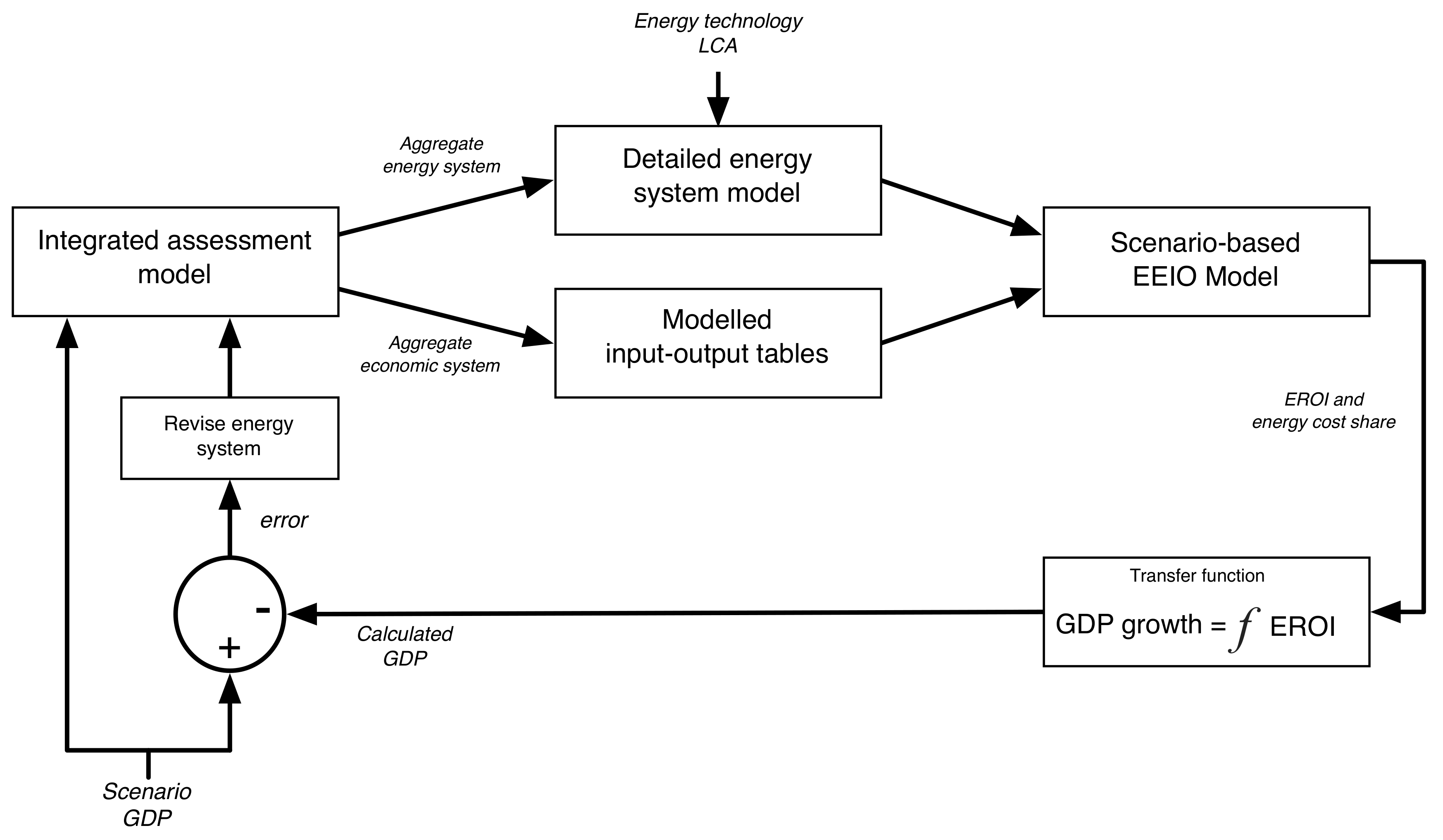
4.1. A Proposed Net-Energy Feedback Model

Net-energy analysis requires estimation of both the direct and indirect energy of energy supply to derive a systematically-complete EIOU for the EROI denominator (see Equation (2)). Where the EROI is sufficiently high (>~20:1) or it is assumed that future energy systems will possess an EROI at least as high as incumbent energy systems, a net-energy approach may not contribute additional information to that already available in IAMs.
A provisional national estimate for EIOU can be derived from the IEA energy balance statistics. The IEA documentation states that ‘Energy industry own use contains the primary and secondary energy consumed by transformation industries for heating, pumping, traction, and lighting purposes, (including) for example, own use of energy in coal mines, own consumption in power plants and energy used for oil and gas extraction.’ Some studies have used the EIOU to calculate EROI at a national level (e.g., Brand-Correa et al. [114], King et al. [115]), but the IEA metric only partly reflects the boundaries usually adopted for the EROI denominator [116]. In 2015, the IEA reported EIOU as 8.9% of total final global consumption ([117], p. 47).
A systematically-complete method of deriving EIOU is environmentally-extended input-output analysis (EEIOA). One technique is to combine the national monetary use-table with the national energy account [116]. EEOIA permits disaggregation of primary fuels from EIOU fuels and final demand and identification of indirect energy pathways. The main weakness of EEIOA is homogeneity, or the assumption that each sector of the economy produces a single, homogeneous good or service. Depending on the dependence of imported fuels and electricity supply capital equipment, a multi-regional model may be necessary.
For scenario analysis based on an IAM, it is necessary to convert the IAM aggregate energy and economic system into a detailed energy model and input-output table. From this, an updated EEIOA is evaluated to calculate a system-EROI (see Figure 1).
From Section 3.1, a significant fraction of total factor productivity growth can be attributed to energy. The proposed model requires a transfer function that links EROI (and energy expenditures’ share of GDP) to growth in GDP. The transfer function is underpinned by Bashmakov’s [118] ‘Three Laws of Energy Transitions’, which was the observation that the energy cost to income ratio tends to converge towards a stable long-term ratio. When the energy costs to GDP ratio is below a given threshold, which Bashmakov defines as less than 11% in OECD countries, energy exhibits a moderate price elasticity. However, when the threshold is exceeded, price reactions to small changes in demand are much higher, and economic growth is hampered. Similarly, Fizaine and Court [119] found that the energy cost share in the United States must be less than 11% for the national economy to exhibit a positive economic growth rate. Fizaine and Court [119] explicitly linked the energy cost share to EROI. Whereas neoclassical economics makes the a priori assumption that output elasticities will mirror cost shares in the economy [120], the BPE perspective is that the output elasticity of energy is much larger than the factor share, and for labour, much smaller [33,121].
A further way to model the transfer function is to adopt an aggregate production function approach. In the macroeconomic module of IAMs, output is determined by an aggregate production function, typically of a Cobb–Douglas, or constant elasticity of substitution (CES) form. For example, MACRO’s production function is a nested CES, comprising capital, labour force, electricity demand and non-electric energy demand ([122], Equation (2)).
However, the IAM choice of production function does not resolve the ‘factor share’ problem. The asymmetry of energy’s output elasticity with respect to factor share is consistent with Bashmakov’s asymmetry of economic growth with respect to energy expenditure cost share. In a recent contribution to addressing the problem, Keen and Ayres [56] developed an energy-augmented production function, including a proof that production (output) and distribution (cost shares) are no longer congruent, arguing that ‘something other than marginal products’ must determine the distribution of income.
Referring to Figure 1, finally, the ‘calculated GDP’ that has been determined by the transfer function is compared with the ‘scenario GDP’, giving an error term, which is used as a basis to revise the energy system. We envisage an iterative process of testing IAMs and revising the energy system accordingly.

4.2. Future Work

The proposed feedback model as depicted here is intended as a preliminary conceptual model. The model as described is technically demanding. IAMs operate at a regional level, but EEIOA is usually modelled at a national level. Multi-regional input output models, such as the Australian Industrial Ecology Virtual Laboratory (IELab) [123], facilitate regional energy-economic modelling and would provide a basis for EEIOA. The transfer function as described requires further work to demonstrate the linkages between energy supply and the economy.

5. Conclusions

Analysis of the costs and benefits of climate mitigation involve extrapolation into the future. However, the long time horizons of interest extend well beyond the range of standard economic-development scenarios. In order to guide policy makers, ‘transformation pathways’ are derived from integrated Assessment Models (IAMs). These models represent interactions between human and natural systems, including energy, agriculture, the carbon cycle and economic systems.
IAMs adopt simplified, stylised and numerical approaches to complex systems. Since the future evolution of demography, socio-economic development and technology are highly uncertain, scenarios have been developed that describe plausible alternative pathways for the key socio-economic drivers of greenhouse gas (GHG) emissions. The drivers can be described by the Kaya identity. The Kaya identity includes population, per-capita income, energy intensity of the economy and carbon intensity of energy. Since the identity is multiplicative, the component growth rates are additive. Therefore, growth of per-capita income is compatible with a decline of GHG emissions, provided energy and carbon intensity decline sufficiently rapidly.
A hypothesis of biophysical economics (BPE) is that per-capita income growth is in fact an emergent parameter from the biophysical-economic system. Rather than being independent variables, the Kaya parameters are interlinked in complex ways. If future energy systems were to possess worse biophysical performance characteristics, we would expect lower productivity and economic growth, and therefore, the price of reaching emission targets may be significantly costlier than projected. With the long time horizons of IAMs, the nature of compound growth means that relatively small differences in economic growth result in a significant divergence in outcomes.
We propose that per-capita income growth is included as a feedback loop in IAMs. One approach would be to use environmentally-extended input-output analysis (EEIOA) to link the biophysical properties of the modelled energy system with projected economic growth. The EEIOA would be based on a detailed energy system model that is constructed from the aggregate model described by the IAM. A transfer function would link the calculated energy cost share, derived from the EEIOA model, to economic growth. Depending on the difference between the exogenous and calculated GDP, the IAM energy system would be revised. The proposed feedback model is intended as a preliminary conceptual model. Further work is required to build a framework that can supplement and support IAM analysis.

Acknowledgments

Thanks to the three anonymous reviewers who have added much to the quality of this article through their insightful comments. Thanks to Igor Bashmakov and the other anonymous reviewers for comments on an earlier version of the draft and to Josh Floyd for discussions and feedback. Thanks also to my supervisors Robert Crawford and Roger Dargaville.

Conflicts of Interest

The author declares no conflict of interest.

Abbreviations

The following abbreviations are used in this manuscript:
AR5IPCC Fifth Assessment Report
CO 2 eqCarbon dioxide equivalent
CSPConcentrated solar thermal power
DNE21+Dynamic New Earth 21 model
EEIOAEnvironmentally-extended input-output analysis
EIOUEnergy industry own use
EMF27Stanford Energy Modeling Forum Study 27
EROIEnergy return on investment
EVElectric vehicle
GEAGlobal Energy Assessment
GDPGross domestic product
IAMIntegrated Assessment Model
IEIndustrial Ecology
IEAInternational Energy Agency
IMAGEIntegrated Model to Assess the Global Environment
IPCCIntergovernmental Panel on Climate Change
ISOInternational Organization for Standardization
LCALife-cycle assessment or analysis
MACROIIASA macroeconomic model
MESSAGEModel for energy supply strategy alternatives and their general environmental impact
MESSAGE-MACROLinked energy supply model (MESSAGE) and macroeconomic model (MACRO)
OECDOrganisation for Economic Co-operation and Development
OPECOrganization of the Petroleum Exporting Countries
POLESProspective outlook on long-term energy systems
RCPRepresentative Concentration Pathways
RERenewable energy
SRESSpecial Report on Emissions Scenarios
WEOIEA World Energy Outlook
WITCHWorld induced technical change hybrid

References

  1. Clarke, L.; Jiang, K.; Akimoto, K.; Babiker, M.; Blanford, G.; Fisher-Vanden, K.; Hourcade, J.; Krey, V.; Kriegler, E.; Loschel, A.; et al. Assessing Transformation Pathways. In Climate Change 2014: Mitigation of Climate Change. Contribution of Working Group III to the Fifth Assessment Report of the Intergovernmental Panel on Climate Change; Cambridge University Press: New York, NY, USA, 2014. [Google Scholar]
  2. Nakicenovic, N.; Alcamo, J.; Davis, G.; De Vries, B.; Fenhann, J.; Gaffin, S.; Gregory, K.; Griibler, A.; Jung, T.Y.; Kram, T. Special Report on Emissions Scenarios; Intergovernmental Panel on Climate Change: Geneva, Switzerland, 2000.
  3. Gupta, S.; Harnisch, J.; Barua, D.C.; Chingambo, L.; Frankel, P.; Jorge, R.; Vázquez, G.; Gomez Echeverri, L.; Haites, E.; Huang, Y. Cross-cutting investment and finance issues. In Climate Change 2014: Mitigation of Climate Change. Contribution of Working Group III to the Fifth Assessment Report of the Intergovernmental Panel on Climate Change; Cambridge University Press: New York, NY, USA, 2014. [Google Scholar]
  4. Krey, V.; Masera, O. Annex II: Metrics and Methodology. In Climate Change 2014: Mitigation of Climate Change. Contribution of Working Group III to the Fifth Assessment Report of the Intergovernmental Panel on Climate Change; Cambridge University Press: New York, NY, USA, 2013. [Google Scholar]
  5. Stern, N. The structure of economic modeling of the potential impacts of climate change: Grafting gross underestimation of risk onto already narrow science models. J. Econ. Lit. 2013, 51, 838–859. [Google Scholar] [CrossRef]
  6. Moyer, E.J.; Woolley, M.D.; Matteson, N.J.; Glotter, M.J.; Weisbach, D.A. Climate impacts on economic growth as drivers of uncertainty in the social cost of carbon. J. Legal Stud. 2014, 43, 401–425. [Google Scholar] [CrossRef]
  7. Smith, K. Discounting, Risk and Uncertainty in Economic Appraisals of Climate Change Policy: Comparing Nordhaus, Garnaut and Stern. Available online: http://www.garnautreview.org.au/update-2011/commissioned-work/smith-discounting-risk-uncertainty-comparing-nordhaus-garnaut-stern.pdf (accessed on 20 June 2017).
  8. Pindyck, R.S. The use and misuse of models for climate policy. Rev. Environ. Econ. Policy 2017, 11, 100–114. [Google Scholar] [CrossRef]
  9. Chevallerau, F.X. What Is Biophysical Economics? Available online: https://biophyseco.org (accessed on 20 November 2017).
  10. Hall, C.A.; Klitgaard, K.A. Energy and the Wealth of Nations: Understanding the Biophysical Economy; Springer Science & Business Media: New York, NY, USA, 2011. [Google Scholar]
  11. Hall, C.A. Energy Return on Investment: A Unifying Principle for Biology, Economics, and Sustainability; Springer: Berlin, Germany, 2016. [Google Scholar]
  12. Lambert, J.G.; Hall, C.A.; Balogh, S.; Gupta, A.; Arnold, M. Energy, EROI and quality of life. Energy Policy 2014, 64, 153–167. [Google Scholar] [CrossRef]
  13. King, C.W. Comparing world economic and net energy metrics, Part 3: Macroeconomic Historical and Future Perspectives. Energies 2015, 8, 12997–13020. [Google Scholar] [CrossRef]
  14. Brandt, A.R.; Dale, M. A general mathematical framework for calculating systems-scale efficiency of energy extraction and conversion: Energy return on investment (EROI) and other energy return ratios. Energies 2011, 4, 1211–1245. [Google Scholar] [CrossRef]
  15. Murphy, D.J.; Hall, C.A. Energy return on investment, peak oil, and the end of economic growth. Ann. N. Y. Acad. Sci. 2011, 1219, 52–72. [Google Scholar] [CrossRef] [PubMed]
  16. Murphy, D.J.; Hall, C.A.; Dale, M.; Cleveland, C. Order from chaos: A preliminary protocol for determining the EROI of fuels. Sustainability 2011, 3, 1888–1907. [Google Scholar] [CrossRef]
  17. King, C.W.; Maxwell, J.P.; Donovan, A. Comparing World Economic and Net Energy Metrics, Part 1: Single Technology and Commodity Perspective. Energies 2015, 8, 12949–12974. [Google Scholar] [CrossRef]
  18. King, C.W.; Hall, C.A. Relating financial and energy return on investment. Sustainability 2011, 3, 1810–1832. [Google Scholar] [CrossRef]
  19. Heun, M.K.; de Wit, M. Energy return on (energy) invested (EROI), oil prices, and energy transitions. Energy Policy 2012, 40, 147–158. [Google Scholar] [CrossRef]
  20. Jacks, D.S. From Boom to Bust: A Typology of Real Commodity Prices in the Long Run; Working Paper No. 18874; The National Bureau of Economic Research (NBER): Cambridge, MA, USA, 2013. [Google Scholar]
  21. Palmer, G.; Floyd, J. An Exploration of Divergence in EPBT and EROI for Solar Photovoltaics. BioPhys. Econ. Resour. Qual. 2017, 2, 15. [Google Scholar] [CrossRef]
  22. Von Hippel, F.; Bunn, M.; Diakov, A.; Ding, M.; Goldston, R.; Katsuta, T.; Ramana, M.; Suzuki, T.; Yu, S. Nuclear Energy. In Global Energy Assessment; Cambridge University Press: New York, NY, USA, 2012. [Google Scholar]
  23. Warner, E.S.; Heath, G.A. Life cycle greenhouse gas emissions of nuclear electricity generation. J. Ind. Ecol. 2012, 16, S73–S92. [Google Scholar] [CrossRef]
  24. Stocker, T.; Qin, D.; Plattner, G.K.; Alexander, L.; Allen, S.; Bindoff, N.; Bréon, F.M.; Church, J.; Cubasch, U.; Emori, S. Technical summary. In Climate Change 2013: The Physical Science Basis. Contribution of Working Group I to the Fifth Assessment Report of the Intergovernmental Panel on Climate Change; Cambridge University Press: New York, NY, USA, 2013. [Google Scholar]
  25. International Institute for Applied Systems Analysis (IIASA). AR5 Scenario Database; IIASA: Laxenburg, Austria, 2014. [Google Scholar]
  26. Edenhofer, O.; Pichs-Madruga, R.; Sokona, Y.; Farahani, E. Summary for Policymakers. In Climate Change 2014: Mitigation of Climate Change. Contribution of Working Group III to the Fifth Assessment Report of the Intergovernmental Panel on Climate Change; Cambridge University Press: New York, NY, USA, 2014. [Google Scholar]
  27. Tol, R.S. On the optimal control of carbon dioxide emissions: An application of FUND. Environ. Model. Assess. 1997, 2, 151–163. [Google Scholar] [CrossRef]
  28. Nordhaus, W.D.; Boyer, J. Warming the World: Economic Models of Global Warming; MIT Press: Cambridge, MA, USA, 2000. [Google Scholar]
  29. Bruckner, T.; Bashmakov, I.; Mulugetta, Y.; Chum, H.; De la Vega Navarro, A.; Edmonds, J.; Faaij, A.; Fungtammasan, B.; Garg, A.; Hertwich, E. Energy systems. In Climate Change 2014: Mitigation of Climate Change. Contribution of Working Group III to the Fifth Assessment Report of the Intergovernmental Panel on Climate Change; Cambridge University Press: New York, NY, USA, 2014. [Google Scholar]
  30. Iyer, G.; Hultman, N.; Eom, J.; McJeon, H.; Patel, P.; Clarke, L. Diffusion of low-carbon technologies and the feasibility of long-term climate targets. Technol. Forecast. Soc. Chang. 2015, 90, 103–118. [Google Scholar] [CrossRef]
  31. Mankiw, N.G. Macroeconomics; Worth Publishers: New York, NY, USA, 2009. [Google Scholar]
  32. Solow, R.M. Technical change and the aggregate production function. Rev. Econ. Stat. 1957, 39, 312–320. [Google Scholar] [CrossRef]
  33. Ayres, R.U.; Warr, B. The Economic Growth Engine: How Energy and Work Drive Material Prosperity; Edward Elgar Publishing Limited: Cheltenham, UK, 2010. [Google Scholar]
  34. Humphrey, T.M. Algebraic production functions and their uses before Cobb-Douglas. FRB Richmond Econ. Q. 1997, 83, 51–83. [Google Scholar]
  35. Grubb, M. Planetary Economics: Energy, Climate Change and the Three Domains of Sustainable Development; Routledge: London, UK, 2014. [Google Scholar]
  36. Krugman, P.R. The Age of Diminished Expectations: US Economic Policy in the 1990s; MIT Press: Cambridge, MA, USA, 1997. [Google Scholar]
  37. Romer, P. Endogenous Technological Change; University of Chicago: Chicago, IL, USA, 1990. [Google Scholar]
  38. Buonanno, P.; Carraro, C.; Galeotti, M. Endogenous induced technical change and the costs of Kyoto. Resour. Energy Econ. 2003, 25, 11–34. [Google Scholar] [CrossRef]
  39. Gillingham, K.; Newell, R.G.; Pizer, W.A. Modeling endogenous technological change for climate policy analysis. Energy Econ. 2008, 30, 2734–2753. [Google Scholar] [CrossRef]
  40. Azar, C.; Dowlatabadi, H. A review of technical change in assessment of climate policy. Annu. Rev. Energy Environ. 1999, 24, 513–544. [Google Scholar] [CrossRef]
  41. Organization for Economic Cooperation and Development (OECD). OECD Compendium of Productivity Indicators 2017; Report; OECD: Paris, France, 2017. [Google Scholar]
  42. Gordon, R.J. The Rise and Fall of American Growth: The US Standard of Living Since the Civil War; Princeton University Press: Princeton, NJ, USA, 2016. [Google Scholar]
  43. Cowen, T. The Great Stagnation: How America Ate All the Low-Hanging Fruit of Modern History, Got Sick, and Will (Eventually) Feel Better: A Penguin eSpecial from Dutton; Penguin: New York, NY, USA, 2011. [Google Scholar]
  44. Summers, L.H. US economic prospects: Secular stagnation, hysteresis, and the zero lower bound. Bus. Econ. 2014, 49, 65–73. [Google Scholar] [CrossRef]
  45. Edenhofer, O.; Lessmann, K.; Bauer, N. Mitigation strategies and costs of climate protection: The effects of ETC in the hybrid model MIND. Energy J. 2006, 27, 207–222. [Google Scholar] [CrossRef]
  46. Rao, S.; Keppo, I.; Riahi, K. Importance of technological change and spillovers in long-term climate policy. Energy J. 2006, 27, 123–139. [Google Scholar]
  47. Sano, F.; Akimoto, K.; Homma, T.; Tomoda, T. Analysis of Technological Portfolios for CO2 Stabilizations and Effects of Technological Changes. Energy J. 2006, 27, 141–161. [Google Scholar] [CrossRef]
  48. Löschel, A. Technological change in economic models of environmental policy: A survey. Ecol. Econ. 2002, 43, 105–126. [Google Scholar] [CrossRef]
  49. Ayres, R. Energy, Complexity and Wealth Maximization; Springer: Berlin, Germany, 2016. [Google Scholar]
  50. Garrett, T.J. Long-run evolution of the global economy: 1. Physical basis. Earth’s Future 2014, 2, 127–151. [Google Scholar] [CrossRef]
  51. Lindenberger, D.; Kümmel, R. Energy and the state of nations. Energy 2011, 36, 6010–6018. [Google Scholar] [CrossRef]
  52. Kumhof, M.; Muir, D. Oil and the world economy: Some possible futures. Philos. Trans. R. Soc. Lond. A Math. Phys. Eng. Sci. 2014, 372. [Google Scholar] [CrossRef]
  53. Kümmel, R.; Lindenberger, D.; Weiser, F. The economic power of energy and the need to integrate it with energy policy. Energy Policy 2015, 86, 833–843. [Google Scholar] [CrossRef]
  54. Kümmel, R. Why energy’s economic weight is much larger than its cost share. Environ. Innov. Soc. Transit. 2013, 9, 33–37. [Google Scholar] [CrossRef]
  55. Giraud, G.; Kahraman, Z. How Dependent Is Growth from Primary Energy? The Dependency Ratio of Energy in 33 Countries (1970–2011); Documents de Travail du Centre d’Economie de la Sorbonne; Maison des Sciences Économiques: Paris, France, 2014. [Google Scholar]
  56. Keen, S.; Ayres, R. A Note on the Role of Energy in Production. Ecol. Econ. 2017. submitted. [Google Scholar]
  57. Barnett, W. Dimensions and economics: some problems. Q. J. Aust. Econ. 2004, 7, 95–104. [Google Scholar] [CrossRef]
  58. US Energy Information Adminstration (EIA). Global Energy Intensity Continues to Decline; EIA: Washington, DC, USA, 2016.
  59. Lightfoot, H.D. Understand the three different scales for measuring primary energy and avoid errors. Energy 2007, 32, 1478–1483. [Google Scholar] [CrossRef]
  60. US Energy Information Adminstration (EIA). International Energy Outlook; Report; US Energy Information Adminstration: Washington, DC, USA, 2016.
  61. Loftus, P.J.; Cohen, A.M.; Long, J.; Jenkins, J.D. A critical review of global decarbonization scenarios: What do they tell us about feasibility? Wiley Interdiscip. Rev. Clim. Chang. 2015, 6, 93–112. [Google Scholar] [CrossRef]
  62. Teske, S. Energy [R]evolution: A Sustainable World Energy Outlook, 3rd ed.; Greenpeace International, European Renewable Energy Council: Amsterdam, The Netherlands; Brussels, Belgium, 2010. [Google Scholar]
  63. Jacobson, M.Z.; Delucchi, M.A. Providing all global energy with wind, water, and solar power, Part I: Technologies, energy resources, quantities and areas of infrastructure, and materials. Energy Policy 2011, 39, 1154–1169. [Google Scholar] [CrossRef]
  64. Hertwich, E.G.; Peters, G.P. Carbon footprint of nations: A global, trade-linked analysis. Environ. Sci. Technol. 2009, 43, 6414–6420. [Google Scholar] [CrossRef] [PubMed]
  65. Crawford, R. Life Cycle Assessment in the Built Environment; Spon Press: Oxfordshire, UK, 2011. [Google Scholar]
  66. Hawkins, T.R.; Singh, B.; Majeau-Bettez, G.; Strømman, A.H. Comparative environmental life cycle assessment of conventional and electric vehicles. J. Ind. Ecol. 2013, 17, 53–64. [Google Scholar] [CrossRef]
  67. Crawford, R.; Stephan, A. The Significance of Embodied Energy in Certified Passive Houses. World Acad. Sci. Eng. Technol. 2013, 78, 589–595. [Google Scholar]
  68. Alcott, B. Jevons’ paradox. Ecol. Econ. 2005, 54, 9–21. [Google Scholar] [CrossRef]
  69. Greening, L.A.; Greene, D.L.; Difiglio, C. Energy efficiency and consumption—The rebound effect—A survey. Energy Policy 2000, 28, 389–401. [Google Scholar] [CrossRef]
  70. Brockway, P.E.; Saunders, H.; Heun, M.K.; Foxon, T.J.; Steinberger, J.K.; Barrett, J.R.; Sorrell, S. Energy rebound as a potential threat to a low-carbon future: Findings from a new exergy-based national-level rebound approach. Energies 2017, 10, 51. [Google Scholar] [CrossRef]
  71. Cullen, J.M.; Allwood, J.M. The efficient use of energy: Tracing the global flow of energy from fuel to service. Energy Policy 2010, 38, 75–81. [Google Scholar] [CrossRef]
  72. Sorrell, S. Reducing energy demand: A review of issues, challenges and approaches. Renew. Sustain. Energy Rev. 2015, 47, 74–82. [Google Scholar] [CrossRef]
  73. Kolstad, C.; Urama, K.; Broome, J.; Bruvoll, A.; Olvera, M.; Fullerton, D.; Gollier, C.; Hanemann, W.; Hassan, R.; Jotzo, F.; et al. Social, Economic, and Ethical Concepts and Methods. In Climate Change 2014: Mitigation of Climate Change. Contribution of Working Group III to the Fifth Assessment Report of the Intergovernmental Panel on Climate Change; Cambridge University Press: New York, NY, USA, 2014. [Google Scholar]
  74. Blanco, G.; Gerlagh, R.; Suh, S.; Barrett, J.; de Coninck, H.; Morejon, C.; Mathur, R.; Nakicenovic, N.; Ahenkorah, A.; Pan, J.; et al. Drivers, Trends and Mitigation. In Climate Change 2014: Mitigation of Climate Change. Contribution of Working Group III to the Fifth Assessment Report of the Intergovernmental Panel on Climate Change; Cambridge University Press: New York, NY, USA, 2014. [Google Scholar]
  75. Sathaye, J.; Lucon, O.; Rahman, A.; Christensen, J.; Denton, F.; Fujino, J.; Heath, G.; Mirza, M.; Rudnick, H.; Schlaepfer, A. Renewable eNergy in the Context of Sustainable Development; Intergovernmental Panel on Climate Change (IPCC): Geneva, Switzerland, 2012.
  76. Daly, H.E.; Scott, K.; Strachan, N.; Barrett, J. Indirect CO2 emission implications of energy system pathways: Linking IO and TIMES models for the UK. Environm. Sci. Technol. 2015, 49, 10701–10709. [Google Scholar] [CrossRef] [PubMed]
  77. Lenzen, M. Errors in conventional and Input Output based Life Cycle inventories. J. Ind. Ecol. 2000, 4, 127–148. [Google Scholar] [CrossRef]
  78. ISO. ISO 14041—Environmental Management—Life Cycle Assessment—Goal and Scope Definition and Inventory Analysis; Report; International Organization for Standardization: Geneva, Switzerland, 1998. [Google Scholar]
  79. ISO. ISO 14040—Environmental Management—Life Cycle Assessment—Principles and Framework; Report; International Organization for Standardization: Geneva, Switzerland, 2006. [Google Scholar]
  80. Jones, C.; Gilbert, P.; Raugei, M.; Mander, S.; Leccisi, E. An approach to prospective consequential life cycle assessment and net energy analysis of distributed electricity generation. Energy Policy 2016, 100, 350–358. [Google Scholar] [CrossRef]
  81. Sullivan, P.; Krey, V.; Riahi, K. Impacts of considering electric sector variability and reliability in the MESSAGE model. Energy Strategy Rev. 2013, 1, 157–163. [Google Scholar] [CrossRef]
  82. Sonnemann, G.; Vigon, B.; Rack, M.; Valdivia, S. Global guidance principles for life cycle assessment databases: Development of training material and other implementation activities on the publication. Int. J. Life Cycle Assess. 2013, 18, 1169–1172. [Google Scholar] [CrossRef]
  83. Pauliuk, S.; Arvesen, A.; Stadler, K.; Hertwich, E.G. Industrial ecology in integrated assessment models. Nat. Clim. Chang. 2017, 7, 13–20. [Google Scholar] [CrossRef]
  84. IEA. Energy Technology Perspectives; Report; International Energy Agency: Paris, France, 2017.
  85. Van Ruijven, B.J.; Van Vuuren, D.P.; Boskaljon, W.; Neelis, M.L.; Saygin, D.; Patel, M.K. Long-term model-based projections of energy use and CO2 emissions from the global steel and cement industries. Resour. Conserv. Recycl. 2016, 112, 15–36. [Google Scholar] [CrossRef]
  86. Hertwich, E.G.; Gibon, T.; Bouman, E.A.; Arvesen, A.; Suh, S.; Heath, G.A.; Bergesen, J.D.; Ramirez, A.; Vega, M.I.; Shi, L. Integrated life-cycle assessment of electricity-supply scenarios confirms global environmental benefit of low-carbon technologies. Proc. Natl. Acad. Sci. USA 2015, 112, 6277–6282. [Google Scholar] [CrossRef] [PubMed]
  87. Hall, C.A.; Lambert, J.G.; Balogh, S.B. EROI of different fuels and the implications for society. Energy Policy 2014, 64, 141–152. [Google Scholar] [CrossRef]
  88. Smith, P.; Bustamante, M.; Ahammad, H.; Clark, H.; Dong, H.; Elsiddig, E.; Haberl, H.; Harper, R.; House, J.; Jafari, M.; et al. Agriculture, forestry and other land use (AFOLU). In Climate Change 2014: Mitigation of Climate Change. Contribution of Working Group III to the Fifth Assessment Report of the Intergovernmental Panel on Climate Change; Cambridge University Press: New York, NY, USA, 2014. [Google Scholar]
  89. Hall, C.A.; Dale, B.E.; Pimentel, D. Seeking to understand the reasons for different energy return on investment (EROI) estimates for biofuels. Sustainability 2011, 3, 2413–2432. [Google Scholar] [CrossRef]
  90. DeCicco, J.M.; Liu, D.Y.; Heo, J.; Krishnan, R.; Kurthen, A.; Wang, L. Carbon balance effects of US biofuel production and use. Clim. Chang. 2016, 138, 667–680. [Google Scholar] [CrossRef]
  91. Ketzer, F.; Skarka, J.; Rösch, C. Critical Review of Microalgae LCA Studies for Bioenergy Production. BioEnergy Res. 2017, 11, 95–105. [Google Scholar] [CrossRef]
  92. Carneiro, M.L.N.; Pradelle, F.; Braga, S.L.; Gomes, M.S.P.; Martins, A.R.F.; Turkovics, F.; Pradelle, R.N. Potential of biofuels from algae: Comparison with fossil fuels, ethanol and biodiesel in Europe and Brazil through life cycle assessment (LCA). Renew. Sustain. Energy Rev. 2017, 73, 632–653. [Google Scholar] [CrossRef]
  93. Agostinho, F.; Ortega, E. Energetic-environmental assessment of a scenario for Brazilian cellulosic ethanol. J. Clean. Prod. 2013, 47, 474–489. [Google Scholar] [CrossRef]
  94. Elliston, B.; Diesendorf, M.; MacGill, I. Simulations of scenarios with 100 percent renewable electricity in the Australian National Electricity Market. Energy Policy 2012, 45, 606–613. [Google Scholar] [CrossRef]
  95. ASEA Brown Boveri (ABB). Power Generation—Energy Efficient Design of Auxiliary Systems in Fossil-Fuel Power Plants; Report; ABB: Zurich, Switzerland, 2009. [Google Scholar]
  96. Edenhofer, O.; Pichs-Madruga, R.; Sokona, Y.; Seyboth, K.; Matschoss, P.; Kadner, S.; Zwickel, T.; Eickemeier, P.; Hansen, G.; Schlömer, S.; et al. Summary for Policymakers. In IPCC Special Report on Renewable Energy Sources and Climate Change Mitigation; Cambridge University Press: New York, NY, USA, 2011. [Google Scholar]
  97. Lu, X.; McElroy, M.B.; Kiviluoma, J. Global potential for wind-generated electricity. Proc. Natl. Acad. Sci. USA 2009, 106, 10933–10938. [Google Scholar] [CrossRef] [PubMed] [Green Version]
  98. Miller, L.M.; Brunsell, N.A.; Mechem, D.B.; Gans, F.; Monaghan, A.J.; Vautard, R.; Keith, D.W.; Kleidon, A. Two methods for estimating limits to large-scale wind power generation. Proc. Natl. Acad. Sci. USA 2015, 112, 11169–11174. [Google Scholar] [CrossRef] [PubMed]
  99. BP. Statistical Review of World Energy 2017; Report; BP: London, UK, 2017. [Google Scholar]
  100. Moriarty, P.; Honnery, D. Can renewable energy power the future? Energy Policy 2016, 93, 3–7. [Google Scholar] [CrossRef]
  101. Dupont, E.; Koppelaar, R.; Jeanmart, H. Global available wind energy with physical and energy return on investment constraints. Appl. Energy 2017, 209, 322–338. [Google Scholar] [CrossRef]
  102. Kubiszewski, I.; Cleveland, C.J.; Endres, P.K. Meta-analysis of net energy return for wind power systems. Renew. Energy 2010, 35, 218–225. [Google Scholar] [CrossRef]
  103. Palmer, G. A Framework for Incorporating EROI into Electrical Storage. BioPhys. Econ. Resour. Qual. 2017, 2. [Google Scholar] [CrossRef]
  104. Rogner, H.H.; Aguilera, R.F.; Bertani, R.; Bhattacharya, S.C.; Dusseault, M.B.; Gagnon, L.; Haberl, H.; Hoogwijk, M.; Johnson, A.; Rogner, M.L.; et al. Energy Resources and Potentials. In Global Energy Assessment—Toward a Sustainable Future; Cambridge University Press: Cambridge, UK; New York, NY, USA, 2012. [Google Scholar]
  105. McCollum, D.; Bauer, N.; Calvin, K.; Kitous, A.; Riahi, K. Fossil resource and energy security dynamics in conventional and carbon-constrained worlds. Clim. Chang. 2014, 123, 413–426. [Google Scholar] [CrossRef]
  106. Rogner, H.H. An assessment of world hydrocarbon resources. Annu. Rev. Energy Environ. 1997, 22, 217–262. [Google Scholar] [CrossRef]
  107. Ritchie, J.; Dowlatabadi, H. Why do climate change scenarios return to coal? Energy 2017, 140, 1276–1291. [Google Scholar] [CrossRef]
  108. Mohr, S.; Wang, J.; Ellem, G.; Ward, J.; Giurco, D. Projection of world fossil fuels by country. Fuel 2015, 141, 120–135. [Google Scholar] [CrossRef]
  109. Rutledge, D. Estimating long-term world coal production with logit and probit transforms. Int. J. Coal Geol. 2011, 85, 23–33. [Google Scholar] [CrossRef]
  110. Capellán-Pérez, I.N.; Arto, I.N.; Polanco-Martínez, J.M.; González-Eguino, M.; Neumann, M.B. Likelihood of climate change pathways under uncertainty on fossil fuel resource availability. Energy Environ. Sci. 2016, 9, 2482–2496. [Google Scholar] [CrossRef]
  111. Mohr, S.H.; Evans, G.M. Forecasting coal production until 2100. Fuel 2009, 88, 2059–2067. [Google Scholar] [CrossRef]
  112. Murray, J.W. Limitations of Oil Production to the IPCC Scenarios: The New Realities of US and Global Oil Production. BioPhys. Econ. Resour. Qual. 2016, 1, 13. [Google Scholar] [CrossRef]
  113. Turner, G.M. A comparison of the Limits to Growth with 30 years of reality. Glob. Environ. Chang. 2008, 18, 397–411. [Google Scholar] [CrossRef]
  114. Brand-Correa, L.; Brockway, P.; Carter, C.; Foxon, T.; Owen, A.; Taylor, P. Developing an Input-Output based method to estimate a national-level EROI (energy return on investment). Energies 2017, 10, 534. [Google Scholar] [CrossRef]
  115. King, C.W.; Maxwell, J.P.; Donovan, A. Comparing World Economic and Net Energy Metrics, Part 2: Total Economy Expenditure Perspective. Energies 2015, 8, 12975–12996. [Google Scholar] [CrossRef]
  116. Palmer, G. An input-output based net-energy assessment of an electricity supply industry. Energy 2017, 141, 1504–1516. [Google Scholar] [CrossRef]
  117. IEA. Key World Energy Statistics—2017; Report; International Energy Agency: Paris, France, 2017.
  118. Bashmakov, I. Three laws of energy transitions. Energy Policy 2007, 35, 3583–3594. [Google Scholar] [CrossRef]
  119. Fizaine, F.; Court, V. Energy expenditure, economic growth, and the minimum EROI of society. Energy Policy 2016, 95, 172–186. [Google Scholar] [CrossRef]
  120. Heun, M.K.; Santos, J.; Brockway, P.E.; Pruim, R.; Domingos, T.; Sakai, M. From theory to econometrics to energy policy: Cautionary tales for policymaking using aggregate production functions. Energies 2017, 10, 203. [Google Scholar] [CrossRef]
  121. Kümmel, R.; Ayres, R.U.; Lindenberger, D. Thermodynamic laws, economic methods and the productive power of energy. J. Non-Equilib. Thermodyn. 2010, 35, 145–179. [Google Scholar] [CrossRef] [Green Version]
  122. Messner, S.; Schrattenholzer, L. MESSAGE–MACRO: Linking an energy supply model with a macroeconomic module and solving it iteratively. Energy 2000, 25, 267–282. [Google Scholar] [CrossRef]
  123. Lenzen, M.; Geschke, A.; Wiedmann, T.; Lane, J.; Anderson, N.; Baynes, T.; Boland, J.; Daniels, P.; Dey, C.; Fry, J. Compiling and using input–output frameworks through collabourative virtual labouratories. Sci. Total Environ. 2014, 485, 241–251. [Google Scholar] [CrossRef] [PubMed]
Figure 1. Proposed biophysical economic feedback model.
Energies 11 00839 g001

