A Network Flow Model for Price-Responsive Control of Deferrable Load Profiles

1
Energy Department, Vlaamse Instelling voor Technologisch Onderzoek (VITO), Boeretang 200, B-2400 Mol, Belgium
2
Energy Department, EnergyVille, Thor Park, Poort Genk 8130, 3600 Genk, Belgium
*
Author to whom correspondence should be addressed.
Energies 2018, 11(3), 613; https://doi.org/10.3390/en11030613
Submission received: 21 December 2017
/
Revised: 2 March 2018
/
Accepted: 6 March 2018
/
Published: 9 March 2018
(This article belongs to the Special Issue Methods and Concepts for Designing and Validating Smart Grid Systems)
Abstract
:This paper describes a minimum cost network flow model for the aggregated control of deferrable load profiles. The load aggregator responds to indicative energy price information and uses this model to formulate and submit a flexibility bid to a high-resolution real-time balancing market, as proposed by the SmartNet project. This bid represents the possibility of the cluster of deferrable loads to deviate from the scheduled consumption, in case the bid is accepted. When formulating this bid, the model is able to take into account the discretized power profiles of the individual loads. The solution of this type of aggregation problems is necessary for the participation of small loads in demand response programs, but scalability can be an issue. The minimum cost network flow problem belongs to a restricted class of discrete optimization problems for which efficient and scalable algorithms exist. Thanks to its scalability, this technique can be useful in the control of a large number of smart appliances in future real-time balancing markets. The technique is efficient enough to be employed by an aggregation module with limited computational resources. Alternatively, when indicative price information is not made available by the system operator, the technique can be combined with an external forecast in order to minimize possible imbalance costs.
1. Introduction
Stimulated by financial and regulatory incentives in an effort to reduce carbon emissions, some countries have experienced rapid growth in renewable energy sources such as wind and solar, which are clean, but intermittent. In order to balance the supply and demand of electrical energy, the power grid relies largely on dispatchable generation provided by conventional hydro- or carbon-based technologies. This balance must be kept at all times.
In the initial stages of the energy transition, not much needed to change, since the larger part of the energy mix still consisted of dispatchable generators. This becomes more difficult in a scenario with a very high penetration of intermittent renewable sources. One possible solution is to provide more flexible and controllable consumption in order to compensate for the loss of controllability on the generation side, in what is called demand response (DR) [1,2]. For the purpose of balancing the power grid, a reduction in power consumption is equivalent to an increase in generation. Conversely, an increase in power consumption is equivalent to a decrease in generation. Demand response can be offered in many forms and traded bilaterally or offered to the best buyer in organized energy markets [3].
More efficient energy markets play an important role in this energy transition. Usually, energy is traded separately for each hourly time slot. The higher volatility arising from short-term uncertainties associated with renewable energy sources increases the importance of energy trading being conducted at smaller time slots and closer to delivery, approximating a continuously-traded real-time market (RTM). Without solving the intrinsic volatility problem, these more refined markets at least do not ignore the intra-hour variations in energy prices, exposing all participants to a price that is as close as it is technically possible to an ideal real-time price. In an ideal scenario, the matching between elastic supply and elastic demand of energy would be achieved at every time slot, and this would mitigate price shocks, with dispatchable generators and flexible consumption adjusting to the fluctuations of renewables, following a price indication that is continuously updated.
Unfortunately, flexible demand participation is not yet the current situation in energy markets, as the large majority of consumers are exposed to a fixed price energy contract, which does not reflect the immediate price signals. Many consumers also lack the smart metering capabilities that would enable them to engage in more dynamic energy contracts with their suppliers. There is a need to improve wholesale energy markets so that more energy retailers and their customers can respond to price signals.
In the meantime, flexibility aggregators arose as a new market player that has more freedom to engage in customized agreements with suitable flexibility providers. The aggregator core business is to manage a flexibility pool large enough and controllable enough to participate in existing balancing reserve programs with the system operators. Alternatively, the aggregator can decide to sell its flexibility to balancing responsible parties (BRPs) under bilateral agreements. There are many possible mechanisms for an aggregator to market its flexibility, but there are also technical problems resulting from the uncoordinated activation of flexibility by different actors. An integrated market framework operating close to real-time could serve as a common platform for all these different actors, which could transact flexibility in a transparent manner and on an equal level.
In the context of the the SmartNet project, such a market is proposed [4] and employed in order to simulate the procurement of flexibility from transmission system operators (TSOs) and distribution system operators (DSOs). Different coordination schemes were proposed, described in detail in the SmartNet deliverable D1.3 [5]. Different aggregator techniques were implemented in the project [6], usually associated with a specific device technology, such as battery storage or combined heat and power (CHPs) units. These aggregation models build on the physical characteristics of a specific device or their aggregated characteristics.
The alternative approach is not to delimit a particular device technology, but to define an abstract model used to represent a number of different devices. In this paper, we focus on a model that represents loads with a fixed power profile, which are non-interruptible, but deferrable. The only way to obtain flexibility from these devices is to defer their activation to a different time.
This model can be useful for incorporating wet appliances as flexible loads controlled by an aggregator. Wet appliances consist of domestic appliances such as washing machines, dishwashers and tumble driers. The power profiles can reflect the dynamics of the device, requesting more or less power at different stages of operation, for instance during the spinning cycle of a washing machine.
Similar concepts are described in the literature with the name of shiftable loads, or deferrable loads with deadlines [7]. However, these models allow a device to reallocate energy consumption between different time slots, provided that the total energy required to complete an associated task is attained before a deadline. Some models also incorporate ramping constraints, charging rates or other device-specific constraints.
In the definition of deferrable load profile adopted in this paper, on the other hand, it is not possible to modify the energy consumption profile of a single device following its activation, which is completely determined by its fixed power profile.
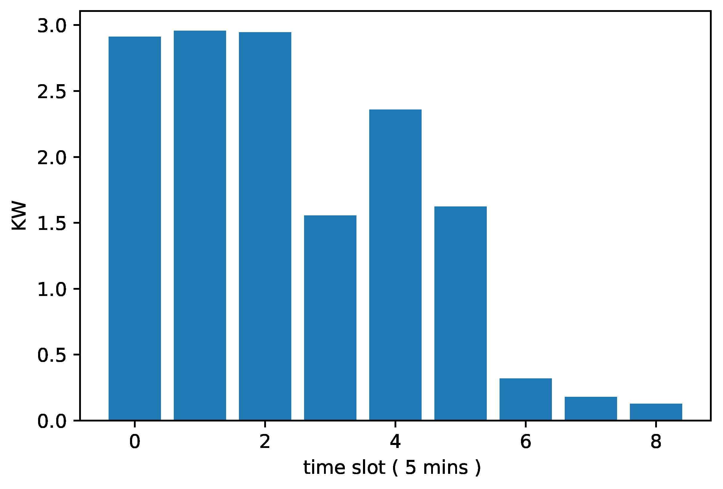
The use of a discrete power profile is motivated by the fine-grained resolution of the SmartNet RTM and the increasing availability of disaggregated home appliance data [8]. We see in Figure 1 a representative power profile for a tumble-dryer. Wet appliances can provide flexibility [9], and the cost is low, provided that the delay in finishing their tasks is tolerable for the users.
In order to handle effectively a large number of loads with similar characteristics, the proposed method groups them by load profile and time of activation and places them in a waiting buffer. This buffer is filled up or emptied according to the objectives of the aggregator and respecting a maximum time delay tolerance. In analogy with a storage device, the aggregator produces flexibility by ‘charging’ or ‘discharging’ a buffer of deferrable loads. Different from energy storage, the decision to charge or discharge the waiting buffer will affect the energy consumption not only in the immediate time slot, but also in subsequent time slots, since each activated load will follow its fixed power profile until its termination.
From a market point of view, large storage capacity would allow energy to be treated as a more persistent commodity. The cumulative effect of aggregators and storage owners buying and storing inexpensive energy in order to be sold at a profit at a more expensive time slot would eventually reduce price swings. This would be beneficial to the stability of the power grid, especially in a scenario with a high penetration of renewable generation. A cluster of shiftable loads is capable of behaving in a similar fashion, while avoiding investment in storage technologies.
In order to keep maximum delays tolerable for the users, the model proposed in this paper will enforce deadlines in each shiftable load. The aggregator will cycle loads in the buffer in order to always have enough stored loads, while preventing loads already waiting in the buffer from exceeding their maximum delay tolerance. At every market iteration, the aggregator will formulate a scheduling plan for the expected incoming loads and the loads already in the buffer. It will be shown that this combinatorial problem is a network flow model that can be solved very efficiently. This is a very useful property, given the large number of participating loads necessary in order to produce flexibility in a volume high enough to participate in energy markets.
Paper Organization
The rest of the paper is organized as follows. In Section 2, we will establish a simplified market design that will be assumed by the load control technique. The imbalance settlement conditions on this simplified market will be reviewed. The deferrable load model used to produce flexibility will be described in more detail. Next, the buffer model used by the aggregator to manage a cluster of deferrable load profiles will be described, with the inputs assumed by the aggregator. Finally, some properties of the network flow model will be reviewed in order to give performance indications of the proposed method.
In Section 3, we will illustrate the buffer model employed by the aggregator using indicative price data from an existing real-time balancing market.
We conclude in Section 4, indicating some future lines of investigation.
2. Proposed Framework
2.1. Assumed Market Design
Electrical energy is traded in successive markets well in advance of physical delivery. Starting from long-term bilateral contracts between energy suppliers and retailers, there is a sequence of time-scales in which energy is traded. This complex structure of cascading markets is important to provide continuous adjustments and updates between the involved market participants, especially in a scenario with a high penetration of renewables.
One of the most important energy markets is the day-ahead market (DAM), which takes place one day before delivery and trades energy for a particular country or region at every given hour slot in the next day. The most prevalent time resolution for the DAM in Europe is 1 h, but in some countries, it is possible to trade energy in the DAM in blocks of 30 min, followed by other more granular trading opportunities in continuous intra-day markets (CIM). These two markets are still evolving, and they are the target of many harmonization initiatives, both EU and industry driven.
As we get closer to real-time, grid congestion might cause a price discrepancy between different nodes of the transmission network. In some regions of the U.S., Canada and in Australia, the market operator offers a last trading possibility in a faster nodal real-time balancing market, featuring a rolling window with 5-min dispatch intervals [10]. These markets are more complicated, but also reflect more accurately the true price of energy at a given node of the network.
Without going into the details of energy markets (see more in [11]), we now present a simplified market design similar to what is proposed in SmartNet. This design strikes a balance between existing mechanisms, adopted for day-ahead energy procurement and imbalance settlement, and the proposed SmartNet RTM [4]. Market design decisions are important since they affect the bidding strategy used by the aggregator.
We assume that our aggregator is a demand response provider that offers flexibility from the activation of aggregated loads. There are different arrangements currently in place for demand-side participation in the energy markets. A review of existing DR programs can be found in [12]. The approach adopted in SmartNet is consistent with [13], which recommends that the best mechanism to put DR into the market is by offering it in real-time markets, on the same level with generation resources, respecting the symmetric treatment between supply and demand.
We assume that the aggregator is responsible for managing a nomination position with the system operator, which means that he/she is associated with a balancing responsible party (BRP), a legal entity expected to submit updated energy nominations and be penalized or compensated later for the discrepancies between reported nominations and the realized consumption. We assume that the aggregator has acquired energy in previous markets, which is in line with the forecast consumption of his/her fixed load consumers and his/her flexible consumers. The demand of the fixed load component can be modeled using conventional load forecasting techniques and will not be considered in this paper. We will only consider consumption forecast of the cluster of shiftable profiles, which is assumed to be controllable.
In any case, close to real time, there will be a mismatch between the total energy consumption and the nominated amounts in each time slot, which represents the amount of energy the aggregator is entitled to consume. Close to real time, we assume that the aggregator is provided with new price information from the system operator, and it will have the opportunity to modify its nomination in a sequence of iterations of a fast real-time market (RTM).
Prices and nominations are managed independently for each time slot. We assume the RTM has a rolling time-window, and at frequent intervals, it offers the possibility to update nominations; as a result of each market clearing, it obtains new prices. We assume that the final price for each time slot will be assumed as the final imbalance price, and it will be used to penalize or compensate the aggregator ex post for any deviations between its final nomination and the final consumption. This final price, however, is only known precisely after the corresponding time slot elapses. The RTM mechanism gives only an indication of it.
In Figure 2, we see a diagram illustrating the successive bidding process. Each row indicates a different iteration of the RTM. The first square indicates the time in which the RTM is running. Each RTM iteration only allows trading to be conducted for the time slots indicated by the lighter squares, which define the current trading window. The current bid is formulated only for the current trading window. At every new market clearing, if the bid is accepted, the nominations of those particular slots are updated.
In the figure, we indicate prices for one particular time slot. Notice that the energy price in the slot gets updated by the iterations of the RTM represented by the first and second rows. In the third row, the RTM last price is assumed to be final, and it is not possible to trade that particular slot anymore. The final imbalance price will be defined ex post.
For simplicity, we ignore time resolution differences, and we assume that previous nominations from the DAM, nomination updates from the RTM iterations and the final imbalance calculations are all provided in the same resolution. Previous nominations from the DAM will be corrected in the RTM iterations.
We assume the aggregator is a price-taker, unable to influence prices. This assumption must be carefully considered in case this market represents a smaller size of market restricted to a particular node of the transmission grid.
We assume that at each market clearing the system operator shares indicative price information, and this can be used as a look-ahead mechanism by the participants. However, when bidding, the participant is always uncertain of the actual clearing prices. When submitting a bid, the participant must assign a price to it. In the case of a bid requesting to buy (sell) energy, the bid will be accepted only if the clearing price of the current iteration is above (below) the clearing price. This process repeats in every market iteration.
In existing RTMs, the market clearing proceeds independently for each time slot. If the aggregator is interested in bidding for a range of slots, there is a risk that some slots get accepted, and some of them do not. To avoid this situation, in the proposed SmartNet market, it is possible to update the nominations in blocks, in what is known as a block bid. In existing markets, block bids are used in the DAM, but not in RTM, given the higher complexity of the market clearing procedure.
We assume that the market clearing uses a “pay-as-clear” mechanism, remunerating all accepted bids according to the same prices. This mechanism provides an incentive for the aggregators to submit their true costs in their bids and simplifies the bid formation process.
For instance, if in Figure 2, in the first iteration of the market, the aggregator bids to buy energy for Slot 7 with a price of 40.0, the bid will be accepted, and the aggregator will pay 32.1, given that this is the clearing price. The new clearing prices are not known at the beginning of that market iteration. If it attempted to buy energy for the same slot in the next price iteration, the aggregator would have paid 34.3. If the bid price were 33, the bid would be accepted if placed in the first market iteration, but it would be rejected if it were placed only in the second market iteration, since clearing prices increased a bit and are now above the bid price.
In another departure from existing RTMs, the gate closure on the SmartNet RTM is sufficiently close to the operation. This allows the aggregator to submit bids requesting nomination changes only a couple of time steps before execution.
2.2. Conditions on Imbalance Settlement
After the last market clearing, indicated in the second row of Figure 2, there can be further adjustments that will include the costs of conventional reserves, depending on the actual net consumption and generation of all participants. This is indicated for one particular time slot in the fourth row of Figure 2. This will be only known ex post and will form the imbalance prices. Any deviations on the part of the aggregator in relation to its last reported nomination, either voluntary or involuntary, will be settled at these prices. The aggregator will get paid for any excess nomination not consumed and will be requested to pay for any energy used in excess of its nomination for a particular slot.
This opens the possibility that the aggregator decides to mobilize its demand response resources in order to collect payments or minimize any charges on him/her in the imbalance settlement, using the imbalance mechanism as a ‘spot market’, even after the last gate closure. This possibility implies that when formulating its bids, the aggregator must take into account the opportunity costs or profits that would result if this flexibility were carried to imbalance.
We will assume that these opportunity costs are used to form the bid price. However, these potential gains expected in the imbalance markets must be properly discounted, since the high price volatility and the lack of information about the final state of the system can expose the participant to losses. We assume that this is an incentive for the aggregator to bid in the RTM and update its nomination, in case the bid is accepted, as opposed to maintaining a deliberate imbalance in relation to a previous nomination.
There are some similarities between the SmartNet proposed RTM and real-time balancing markets currently in operation in the U.S. and other countries. Each one of these existing markets, however, has its own design choices and limitations.
Ercot is the ISO responsible for managing most of Texas, and it allows load participation in its real-time security-constrained economic dispatch (SCED) market. Ercot publishes indicative price information for the SCED, which we will use in the next sections to illustrate the proposed technique used by the aggregator on the control of deferrable load profiles.
2.3. Deferrable Load Profile Representation
There are different definitions of responsive loads in the literature. As described briefly in Section 1, we adopted a more restricted definition of load flexibility where the load profiles are fixed, the loads are non-interruptible and only the choice of the time of activation of the device can provide flexibility. In [14], this kind of flexible load is defined as a shiftable profile. In [15], this shiftable load model is classified as non-interruptible and deferrable. Most studies do not consider the shape of these flexible loads, either considering the load profile as any profile that delivers a certain amount of energy before a deadline or as a constant power profile. The choice of a model with a discrete power profile representation suits the resolution of the RTM implemented in SmartNet, which is assumed to use 5-min time slots.
The strategy employed by the aggregator to manage a cluster of loads expected to arrive at different times of the day is to build a buffer of loads, and this buffer is “charged” or “discharged” in order to reduce or increase the power demand for one or more time slots. At the beginning of the bid construction, we assume the buffer has some loads present on it, in order to have some discharge power. Opposite the battery system, the discharge of this buffer will increase the energy consumption. The process is complicated by the inter-temporal power profile of the device.
Other works, such as [15], employ shiftable loads in the context of a residential consumer reacting to real-time energy prices. The small scale of the planning problem allows each deferrable device to be modeled individually, for every possible starting position. The difference in this work is that the aggregator possibly controls hundreds of similar devices arriving at the same time slot and is still able to solve a combinatorial problem efficiently by using the network model described in in Section 2.5. This model will cluster together devices that arrive in each time slot and will provide an optimal load activation schedule in relation to the latest price information.
As happens in general for shiftable loads, the flexibility possible with this kind of device is not easily translated to the interfaces offered by current market design. The value of a task spanning several time steps is associated with the completion of the task, and not its individual energy consumption slots. Current market design usually requires that the participants submit independent price/quantity pairs for each slot.
Shiftable profiles, as well as other sources of flexibility exhibit strong inter-temporal constraints that cannot be easily represented by independent price and quantity pairs. In order to solve this, the proposed SmartNet RTM supports a number of complex bids [4], which we will adopt instead of dealing with the stochastic problems usually employed in optimal bidding [7,16,17].
In this paper, we will focus on a block bid, a bid in which nomination updates at different time slots are submitted together in the same bid, and accepted or rejected in block by the market operator. We will assume the bid is discrete and non-curtailable, that is it cannot be accepted in a fraction. Current market design usually requires bids to be curtailable, being partially accepted within an informed range. We also assume that the price of this update can be established for the whole block, a condition that is similar to minimum income constraints employed in some DAMs. The market clearing procedure is free to accept or reject the whole block. This bid is, however, quite restrictive, and it adds more complexity to the market clearing algorithms utilized by the market operator.
2.4. Initial Setup of Deferrable Load Profiles
The initial setup is as follows. The aggregator starts planning for the current trade window taking into account loads that arrived in a previous iteration of the RTM, but remained inactive. These units were directed to a buffer, to a slot corresponding to their remaining allowed delay, and will now be scheduled to a compatible time slot. The aggregator also estimates the number of deferrable loads that will be joining in the current trade window. These loads, likewise, will be rescheduled to a compatible time slot or carried to the next iteration. Loads can be activated as soon as they join the system, up to a maximum delay .
The current trade window is assumed to have length . For simplicity, we assume that . We assume in this paper homogeneous loads with a fixed load profile , with for . We use to represent the length of the power profile, and we assume that .
We will assume that at the start of a new iteration of the RTM, the buffer has enough loads in order to allow a flexibility bid to be formulated in both directions. An empty buffer, for instance, would only allow downward flexibility to be offered in the first time slots. A half-full buffer would allow both directions to be offered.
Our initial data are summarized in Table 1. For simplicity, the index ranges are relative to the time step in which the market is running.
The most important input is represented by , which should contain the indicative prices from a previous real-time market iteration. We assume that this price information extends beyond the end of the current window in order to estimate costs from imbalances carried beyond the currently traded time window. For instance, loads starting in the last time slot at will extend a power profile of size outside of the currently traded time window.
We assume that the planning is deterministic and that contains the expected number of loads to join in every time slot. In reality, the number of loads joining the system will be random, and this will cause an imbalance position, which can be mitigated by the use of the cluster flexibility. For simplicity, we will not deal with this important aspect in this paper.
The buffer slots keep track of the number of loads that arrived before the current trading window and are waiting to be activated. Deferred loads in the buffer are sorted according to arrival time, with the index s indicating the remaining delay tolerated by loads in that buffer slot. All loads in , for instance, must be immediately activated, since they have already waited the maximum allowed delay, .
The nomination at the beginning of the current bidding comes from the energy bought in the DAM. This nomination vector gets modified by successive iterations of the RTM, as established in Section 2.1.
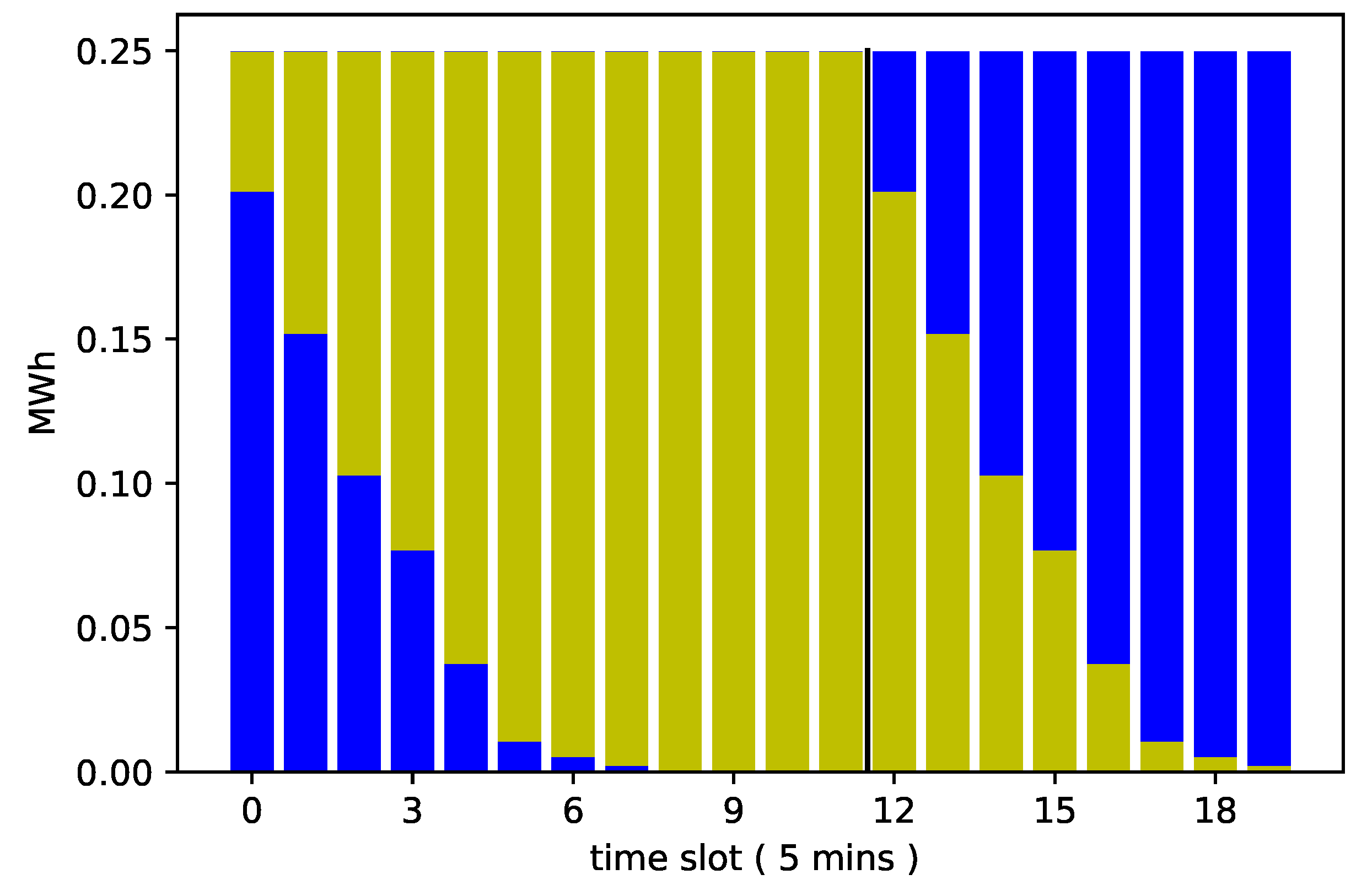
Most of the energy nomination reserved for the day is already committed to loads activated before the current market iteration. In Table 2 a distinction is made between the total nomination and the controllable nomination, still available to be changed. In Figure 3, the controllable nomination is indicated by the lighter bars, represented by . The figure illustrates a market iteration at Time Step 222. The trading window is indicated by the black vertical lines. Past the trading window, there is still controllable nomination corresponding to consumption that can still change depending on the scheduling performed in the current market iteration. Finally, we have a section of the nomination vector indicated by darker bars that represents the consumption of loads expected to arrive only after the end of the trading window.
The buffer starts the current market iteration with a certain distribution of units in different slots. In Table 3, we define variables to model the flow of scheduled loads between the initial state of the buffer and the planned schedule. This model is going to be used in the bid formulation to modify . The variables define how the units waiting in the buffer or expected to arrive in the current time window will be distributed between possible times of activation. In the next section, we will show that this formulation is a type of network flow problem.
In a network problem formulation, we have arcs that connect compatible nodes. In the definition of , it is only necessary to consider the case with . Loads from the buffer slot , for instance, must be activated immediately, while loads from the buffer slot can be scheduled to .
In the definition of , loads expected at time slot u can only be rescheduled at a future time slot that does not exceed the maximum delay .
Finally, as explained for , part of the loads arriving at slots u will be able to replenish a buffer slot corresponding to the remaining delay that the load can tolerate. Loads arriving in slot u can be directed to the buffer slot .
It is convenient to define auxiliary expressions for the final buffer state and the number of loads scheduled to start at a given time slot t. It is also useful to define an expression for the energy flexibility in relation to all possible load rescheduling. These are defined in Table 4.
2.5. Flow-Based Formulation for the Flexibility
With the variables defined in the previous section, we proceed to define a flow-based model, which will allow us to modulate the flexibility profile according to the indicative price signal.
To avoid the complexity of working with indices, we define and indicating compatible arcs by the pairs and , respectively.
The edge set represents the connections between compatible buffer indices s and the time slots t in which they can be scheduled to activate. The edge set plays the same role for incoming loads that are being rescheduled to a future time step in the current time window. We can link the auxiliary expressions with the main variables through the following expressions:
In (3), for each final buffer slot s, there is a unique arrival time responsible for the loads that contribute to it. Unscheduled loads will replenish the buffer and recover the system for a next market iteration.
The loads activated at t, represented in (4), come from two sources. They are either coming from the buffer or from loads arriving in the current window, and in both cases, they are constrained by the tuple sets and .
In (5), we define our most important auxiliary expression, characterizing the energy flexibility in terms of the main variables. The number N represents the number of time slots in one hour, necessary to make the conversion from the power profiles to an energy consumption profile.
In order to simplify the summation, we assume that is extended with zeros. We see that the power profile of a cluster of similar devices is the convolution of the power profile of one device with the activation schedule represented by .
The expression for will be expanded as a linear cost in the objective function of the bid construction problem that follows. The objective function will have a fixed component and terms that depend only on the main variables and .
In (6) and (7), we require that the loads in the waiting buffer and the loads expected to arrive are spread into arcs that lead to compatible time slots.
The term in (7) can be seen as a remainder. Incoming loads not scheduled to be activated in some compatible time slot will replenish the final state buffer, as already indicated in (3).
In (8), we restrict the search of flexibility profiles within those reschedules that put the final buffer in the same condition as the starting buffer. These cyclic boundary conditions will prevent the bidding process from exploiting the buffer in order to maximize the value of the current bid, while compromising its availability in future market iterations.
Notice that in the objective function, some of the imbalance is expected in time slots beyond the end of the current time window. These extra costs (or profits) represented by will not be included in the current bid, but will be carried as a future loss (or future gains) by the aggregator. The other part, represented by , can be seen as opportunity costs arising from the provision of flexibility and will be used to form the cost of the bid. By doing so, the aggregator is proposing to update the nomination vector in that range, provided that the payment is larger than what it expects to obtain in imbalance settlement.
2.6. Network Flow Properties
The problem is uncapacitated, that is there are no constraints on the amount of “flow” through the arcs, apart from requiring that the flow is positive, with . In (10), is positive at source nodes and negative at sink nodes. The “sources” in our formulation represent available loads expected in the current window or drawn from the buffer. The flow represents the rerouting of these units, and the “sinks” represent the desired final buffer added with one artificial sink.
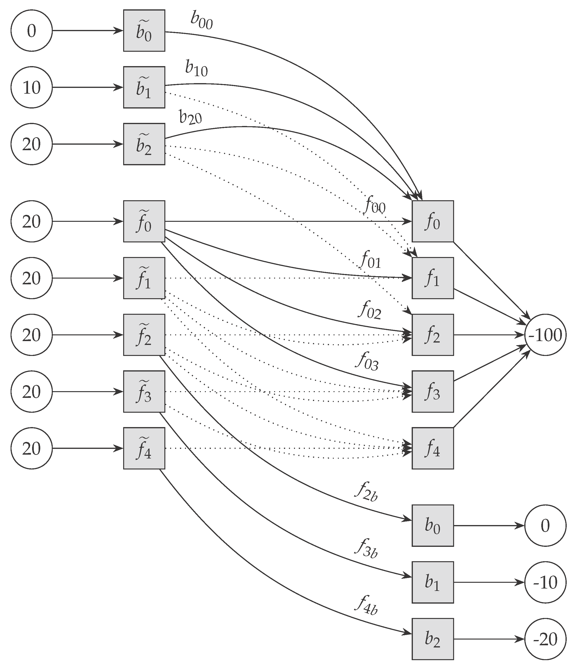
In Figure 4, we display the corresponding network for the bid planning problem described in Section 2.5 for a small example where and .
The sources and sinks are represented by circles, and intermediary nodes are represented with square nodes and maintain zero balance. The costs on the arcs can be obtained from the expansion of in terms of , , . No costs are associated with arcs connecting the square nodes and the circular ones.
Assuming that the problem described is feasible, the integrality theorem on network flows, summarized in Proposition 5.6 in [18], states that since values on sources and sinks are integers, so we will have a primal integer solution for this problem even without imposing integrality constraints explicitly, as in Equations (9) or (11).
This means that although our problem was originally formulated as an integer problem, because of its characteristics, it can be solved directly on its relaxed version, with continuous variables, using any available linear programming solver, or even a specialized network solver. In other words, there is no error introduced by solving the relaxed problem.
In complexity terms, linear programming can be solved in polynomial time, while general integer programming is NP-complete. Network flow algorithms sit in the intersection of these two classes of problems [19].
Mixed integer programming (MIP) solvers generally start by solving the relaxation of the problem, using linear programming, and then proceed to branching and other techniques to solve the problem under integrality constraints. Since as a network flow, we obtain integral solutions automatically, the MIP solver will solve the problem in its relaxed form, avoiding branching entirely.
Even if an MIP solver is used, the problem will be recognized as LP. This gives a good guarantee that the problem will scale well in relation to the number of devices and profiles. On a more practical note, this also gives the option to replace the MIP solver with a more available LP solver.
State-of-the-art MIP solvers are proprietary and expensive software components and because of their computational requirements and high licensing costs may also not be suitable to be deployed in all applications, for instance in embedded systems.
3. Example of the Application of the Proposed Framework
In this section, we use price data from an existing real-time market to illustrate the framework described in the previous section. As described in Section 2.1, the system operator clears the market at periodic intervals. This refreshes an indicative price curve that is used by the aggregator in order to formulate a new flexibility bid. This comes from a new schedule of the cluster of shiftable profiles, found using the network flow method described in Section 2.5. The aggregator will maximize the value of its flexibility by transferring energy consumption from expensive slots to less expensive slots, while respecting the constraints of the model.
There will be a price evolution, and at each new market clearing, the aggregator reformulates a new bid, taking into account any previously accepted bids, as well as the new price information.
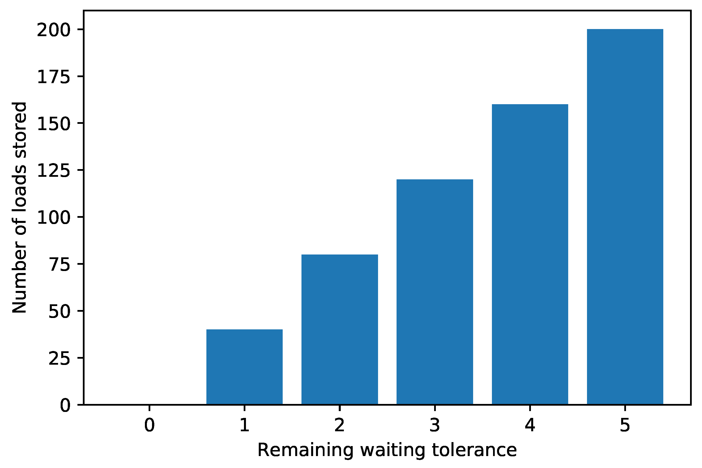
In this example, we assume as the length of the cleared time window and as the maximum allowed delay. We assume that 200 devices arrive at each time slot, all with the same power profile as displayed in Figure 1. The total expected nomination available to be traded is indicated by the lighter bars in Figure 5. This power consumption is limited to load activation decisions that are currently taking place. The darker bars represent consumption corresponding to load activations that already happened or that are beyond the currently traded window. In Figure 6, we show the initial state of the buffer, with the number of waiting units, sorted by the remaining waiting tolerance and the number of time steps they are still allowed to wait before being activated. For instance, Figure 6 indicates that there are 200 loads that are allowed to wait a further five time steps before being activated.
We use indicative price data from Ercot to demonstrate the construction of the flexibility profile, later converted to a block bid. The data are relative to the South Hub, and it was logged on 17 October 2017. In Figure 7, we show indicative price curves collected after sequential market iterations at 18:30, 18:45, 19:00 and 19:15. Each clearing provides prices for each of the 5-min slots, one hour ahead of the collection time. In the absence of price information for the subsequent steps, we assume a simple constant extrapolation. This may be necessary in order to estimate the costs of the imbalances past the current range.
As time evolves, a new market iteration will produce new prices. The new market iteration includes the bid of this aggregator and other bids, representing different aggregators, as well as conventional balancing resources. Price information of future slots is revised up or down, depending on the clearing results. This will also keep extending the range of available data.
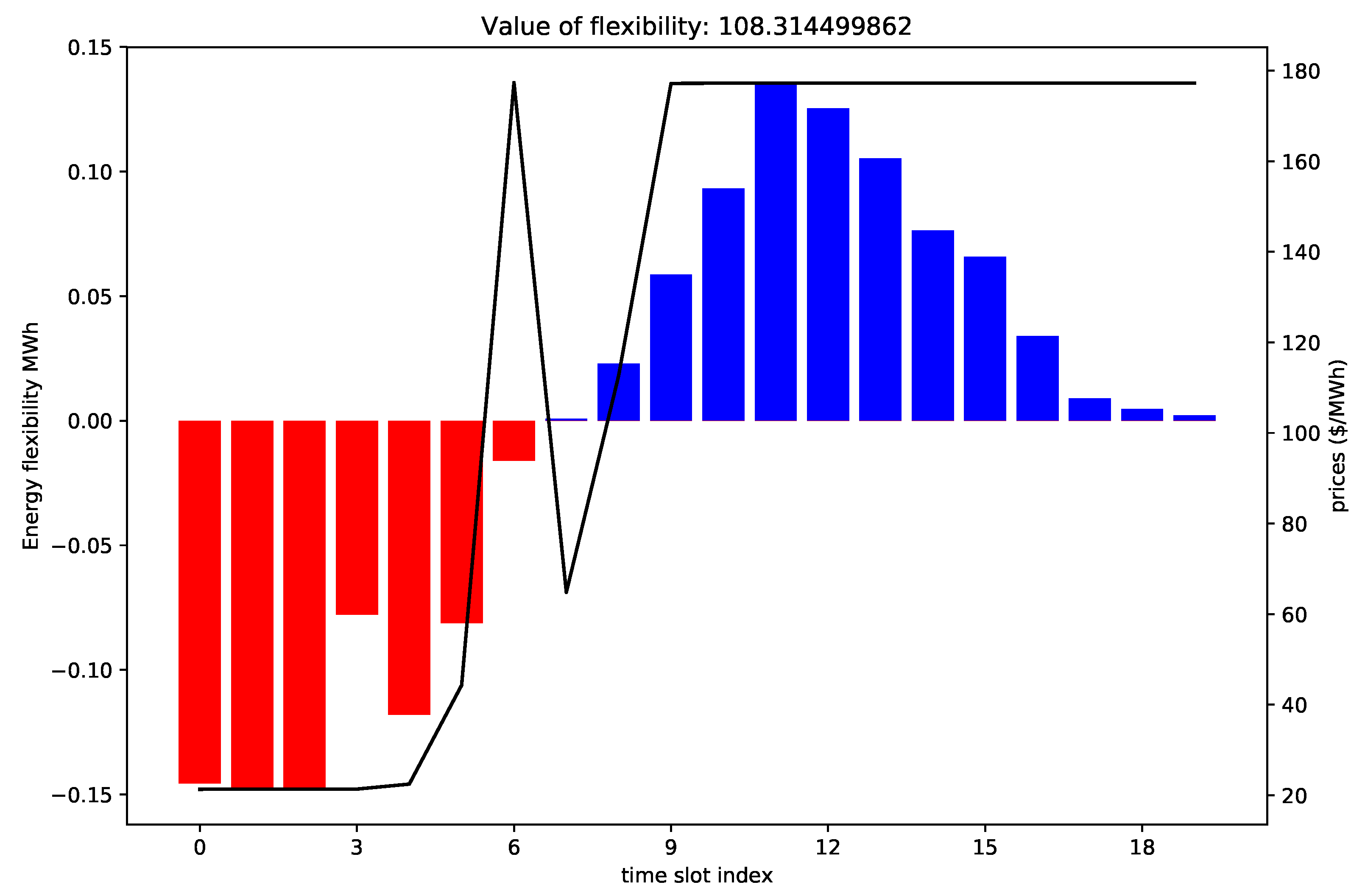
The aggregation will produce one flexibility bid at each iteration, and the price volatility is expected to be managed by successive corrections. The data from 18:30, exhibited in Figure 7, indicate that the system operator was expecting a price spike to happen at 19:00 and then again at 19:15. Based on this first information, the aggregator formulates a load activation schedule that shifts consumption away from the most expensive slots.The flexibility profile is represented in Figure 8. Indices are relative, with the first price peak corresponding to Slot 6.
The sign convention follows the logic that positive flexibility represents more generation. In the case of demand response, this is equivalent to less consumption, indicated in Figure 8 by the blue bars at the end. Negative flexibility corresponds to less generation, which in the case of demand response corresponds to more consumption.
Figure 8 shows that the aggregator uses the price information from 18:30 to propose an increase in immediate energy consumption, before the price spike arrives. In the final slots in blue, the aggregator is proposing a reduction in energy consumption. Energy consumption was anticipated for the first slots.
Similar to Figure 4, from the solution of the problem in (6)–(9), we obtain the corresponding network flow variables that give the aggregator the number of units to reschedule from each time slot to other compatible time slots.
The selected Ercot data in Figure 7 display a period where price volatility is particularly high. The price peak predicted at 19:00 was actually mitigated. At 18:45, the system operator revealed a new price curve, which shows a price of 40 /MWh. The final price information collected after the market iteration at 19:00 is even lower.
If this flexibility profile were to be carried as imbalance by the aggregator instead of offered in the RTM, the aggregator would be exposed to the price volatility of the final imbalance prices, and its managed imbalance position could quickly turn into losses. By offering this profile in the RTM instead, the aggregator will have the opportunity to collect a payment, in case the bid is accepted. In this case, its nominations will be updated, and no imbalance will be due if it follows this new baseline strictly.
There is one limitation, however. Since the traded window is limited to one hour, part of the flexibility will not be included in the current iteration of the market.
Since this flexibility would potentially present potential gains (or losses) to the aggregator in the imbalance settlement, the aggregator can use this value as a reference when forming its own bid price. The value must be discounted, and the discounting factor should be suitably modified to reflect the uncertainty of this outcome.
The flexibility profile is ideally submitted as a block bid and with a single price associated with it. If prices in the current market iteration provide advantageous for the system operator to accept this bid, the aggregator will receive a value at least as high as requested, following the pay-as-clear mechanism.
In that case, the aggregator will update its nominations with the system operator. If the aggregator further departs from the updated nominations, it will be penalized according to the final imbalance prices, but taking into account this new updated nominations. If, on the other hand, the bid is not accepted, the aggregator imbalances will still be calculated in relation to the previous nominations.
In the next market iterations, the aggregator is free to form new flexibility offers, to risk accumulating a favorable imbalance position or to reschedule his/her loads in order to reduce his/her own residual imbalance position, if any.
4. Conclusions
The work developed in this paper demonstrates a simple network flow model that can be used to control a cluster of deferrable load profiles in relation to an indicative price signal. The indicative price curve induces periods of lower consumption when indicative prices are higher or vice versa.
We assumed a market design that allows for frequent market clearing that keeps the participants in a close loop with the system operator. This is one possible future market design simulated in SmartNet.
The aggregator uses the network flow model to form a block bid. If the bid is accepted, the aggregator receives a payment and reschedules its load activations in order to follow a new updated nomination. The energy consumption profile will change according to prices indicated by the RTM.
This bid takes into account the discrete power profiles of each individual load and their interruptibility. The network flow model also prevents loads from waiting longer than a maximum time delay.
If the bid is rejected, the aggregator uses the indicated price curve as indication of the imbalance prices and reschedules its loads in order to maintain a favorable imbalance position.
Existing real-time balancing markets are much simpler and asymmetric than the market proposed in SmartNet. The computational burden and the operational constraints of the system operator require that bids are submitted ahead of the current time window being traded, from 45 min to more than one hour. On the other hand, every 5 min, a different quantity is cleared and expected from the aggregators, which need to react in real-time. Complex bids are not available, and usually, there are no block bids and other more computationally-expensive bids. This requires the aggregator to submit a dispatchable bid, signaling to the market its range of capabilities. The construction of a more dispatchable bid requires a different set of techniques than the model exposed here.
Acknowledgments
This research was conducted by Vito-EnergyVille for the SmartNet project. The SmartNet project was funded by the European Union’s Horizon 2020 research and innovation program under Grant Agreement No. 691405. This paper reflects only the author’s view, and the Innovation and Networks Executive Agency (INEA) is not responsible for any use that may be made of the information it contains.
Author Contributions
J.C. developed the network flow model and wrote the paper. In the course of the project associated with this paper, the model received contributions from F.S. and C.H. The implementation was done in Pyomo/Cplex by J.C. with contributions from C.H.
Conflicts of Interest
The authors declare no conflict of interest.
References
- Eurelectric. Designing Fair and Equitable Market Rules for Demand Response Aggregation; Eurelectric: Brussels, Belgium, 2015; pp. 1–24. [Google Scholar]
- Albadi, M.H.; El-Saadany, E.F. Demand response in electricity markets: An overview. In Proceedings of the 2007 IEEE Power Engineering Society General Meeting, PES, Tampa, FL, USA, 24–28 June 2007; pp. 1–5. [Google Scholar]
- ERCOT. Load Participation in the ERCOT Nodal Market; ERCOT: Austin, TX, USA, 2015. [Google Scholar]
- Ashouri, A.; Sels, P.; Leclercq, G.; Devolder, O.; Geth, F.; D’hulst, R. SmartNet—Network and Market Models: Preliminary Report (D2.4). 2017. Available online: http://smartnet-project.eu/wp-content/uploads/2016/03/D2.4_Preliminary.pdf (accessed on 21 December 2017).
- Gerard, H.; Energyville, V.; Rivero, E.; Energyville, V.; Six, D.; Energyville, V. Basic Schemes for TSO-DSO Coordination and Ancillary Services Provision. 2017. Available online: http://smartnet-project.eu/wpcontent/uploads/2016/12/D1.3_20161202_V1.0.pdf (accessed on 21 December 2017).
- Dzamarija, M.; Plecas, M.; Jimeno, J.; Marthinsen, H.; Camargo, J.; Sánchez, D.; Spiessens, F.; Leclercq, G.; Vardanyan, Y.; Morch, A.; et al. SmartNet—Smart TSO-DSO Interaction Schemes, Market Architectures and ICT Solutions for the Integration of Ancillary Services from Demand Side Management and Distributed Generation Aggregation Models: Preliminary Report, 2017. Available online: http://smartnet-project.eu/wp-content/uploads/2017/06/D2.3_20170616_V1.0.pdf (accessed on 21 December 2017).
- Mohsenian-Rad, H. Optimal demand bidding for time-shiftable loads. IEEE Trans. Power Syst. 2015, 30, 939–951. [Google Scholar] [CrossRef]
- Pipattanasomporn, M.; Kuzlu, M.; Rahman, S.; Teklu, Y. Load profiles of selected major household appliances and their demand response opportunities. IEEE Trans. Smart Grid 2014, 5, 742–750. [Google Scholar] [CrossRef]
- Cardinaels, W.; Borremans, I. Demand Responde for Families—LINEAR Final Report; EnergyVille: Genk, Belgium, 2014. [Google Scholar]
- Vlachos, A.G.; Biskas, P.N. Demand Response in a Real-Time Balancing Market Clearing with Pay-As-Bid Pricing. IEEE Trans. Smart Grid 2013, 4, 1966–1975. [Google Scholar] [CrossRef]
- Kirschen, D.S.; Strbac, G. Fundamentals of Power System Economics; John Wiley & Sons: Chichester, UK, 2004. [Google Scholar]
- Faria, P.; Vale, Z. Demand response in electrical energy supply: An optimal real time pricing approach. Energy 2011, 36, 5374–5384. [Google Scholar] [CrossRef]
- Bushnell, J.; Hobbs, B.F.; Wolak, F.A. When it comes to Demand Response, is FERC its Own Worst Enemy? Electr. J. 2009, 22, 9–18. [Google Scholar]
- Ottesen, S.O.; Tomasgard, A. A stochastic model for scheduling energy flexibility in buildings. Energy 2015, 88, 364–376. [Google Scholar] [CrossRef]
- Chen, Z.; Wu, L.; Fu, Y. Real-time price-based demand response management for residential appliances via stochastic optimization and robust optimization. IEEE Trans. Smart Grid 2012, 3, 1822–1831. [Google Scholar] [CrossRef]
- Conejo, A.J.; Nogales, F.J.; Arroyo, J.M. Price-taker bidding strategy under price uncertainty. IEEE Trans. Power Syst. 2002, 17, 1081–1088. [Google Scholar] [CrossRef]
- Kohansal, M.; Mohsenian-Rad, H. Price-maker economic bidding in two-settlement pool-based markets: The case of time-shiftable loads. IEEE Trans. Power Syst. 2016, 31, 695–705. [Google Scholar] [CrossRef]
- Bertsekas, D. Network Optimization: Continuous and Discrete Models; Athena Scientific: Belmont, MA, USA, 1998. [Google Scholar]
- Papadimitriou, C.H.; Steiglitz, K. Combinatorial Optimization: Algorithms and Complexity; Prentice Hall: Englewood Cliffs, NJ, USA, 1982. [Google Scholar]
Figure 1.
GE-WSM2420D3WW power profile.

Figure 2.
The rolling window mechanism.
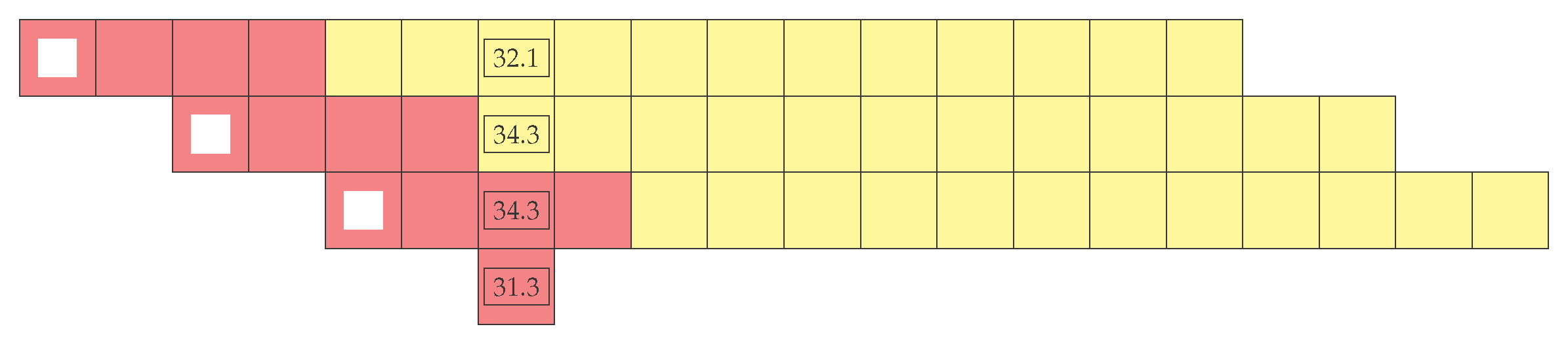
Figure 3.
Controllable and non-controllable nomination.
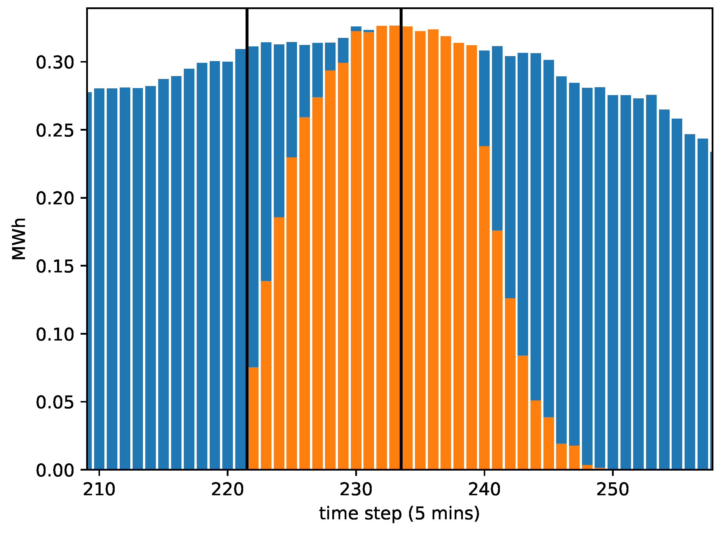
Figure 4.
Network flow model for the flexibility bid.

Figure 5.
Controllable and non-controllable nomination.

Figure 6.
Initial buffer state.

Figure 7.
Ercot indicative prices at the South Hub.
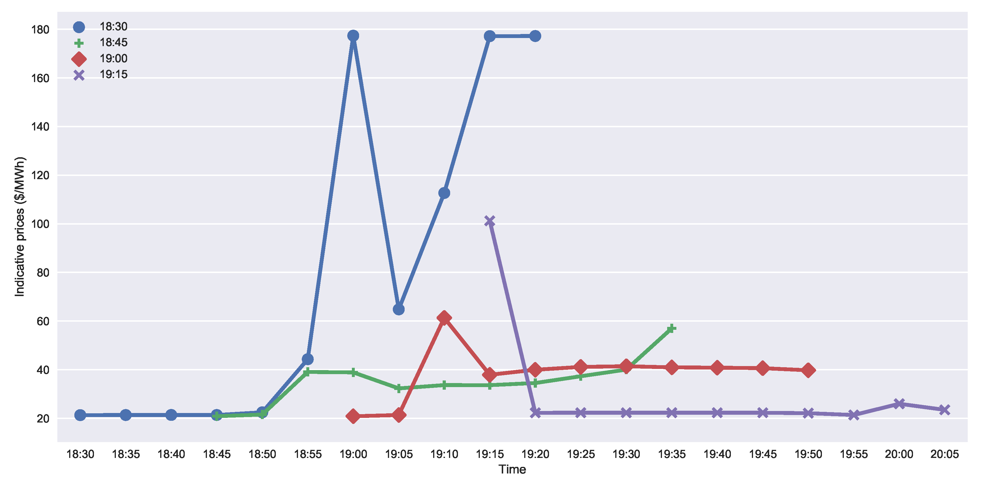
Figure 8.
Imbalances allowed beyond the current time window.

Table 1.
Initial data.
| Input Data | Description |
|---|---|
| Price information | |
| Number of loads expected to join | |
| Number of loads in buffer slot |
Table 2.
Initial nomination data.
| Input Data | Description |
|---|---|
| Total nomination with | |
| Controllable nomination |
Table 3.
Main variables.
| Variables | Description |
|---|---|
| Number of loads in the buffer slot s scheduled to be activated in time slot t, , | |
| Number of loads expected in time slot u rescheduled to a time slot t, with , | |
| Number of loads expected in the time slot u that will be used to replenish the buffer, with |
Table 4.
Auxiliary expressions.
| Auxiliaries | Description |
|---|---|
| Number of loads assigned to final buffer slot s with | |
| Auxiliary variable containing the number of loads activated in slot t of the rolling window, with | |
| Energy consumption flexibility at each time slot t, with |
© 2018 by the authors. Licensee MDPI, Basel, Switzerland. This article is an open access article distributed under the terms and conditions of the Creative Commons Attribution (CC BY) license (http://creativecommons.org/licenses/by/4.0/).
Share and Cite
MDPI and ACS Style
Camargo, J.; Spiessens, F.; Hermans, C. A Network Flow Model for Price-Responsive Control of Deferrable Load Profiles. Energies 2018, 11, 613. https://doi.org/10.3390/en11030613
AMA Style
Camargo J, Spiessens F, Hermans C. A Network Flow Model for Price-Responsive Control of Deferrable Load Profiles. Energies. 2018; 11(3):613. https://doi.org/10.3390/en11030613
Chicago/Turabian StyleCamargo, Juliano, Fred Spiessens, and Chris Hermans. 2018. "A Network Flow Model for Price-Responsive Control of Deferrable Load Profiles" Energies 11, no. 3: 613. https://doi.org/10.3390/en11030613
Note that from the first issue of 2016, this journal uses article numbers instead of page numbers. See further details here.