Automatic Identification of Fractures Using a Density-Based Clustering Algorithm with Time-Spatial Constraints


1
Key Laboratory of Shale Gas and Geoengineering, Institute of Geology and Geophysics, Chinese Academy of Sciences, Beijing 100029, China
2
Institutions of Earth Science, Chinese Academy of Sciences, Beijing 100029, China
3
University of Chinese Academy of Sciences, Beijing 100049, China
*
Author to whom correspondence should be addressed.
Energies 2018, 11(3), 563; https://doi.org/10.3390/en11030563
Submission received: 23 January 2018
/
Revised: 26 February 2018
/
Accepted: 1 March 2018
/
Published: 6 March 2018
(This article belongs to the Special Issue Unconventional Natural Gas (UNG) Recoveries 2018)
Abstract
:In shale gas hydraulic fracture monitoring or rock acoustic emission experiments, fracture plane identification is always a complex task. Conventional approaches typically use the source locating results derived from the micro-seismic event and then interpret the fracture plane using manual qualitative analysis. Large errors typically occur due to manual operations. On the other hand, the density-based clustering algorithm with spatial constraints is widely used in geographic information science, biological cells science and astronomy. It is an automated algorithm and can achieve good classification results. In this paper, we introduced the above-mentioned clustering algorithm with spatial constraints to fracture identification applications. Moreover, because micro-seismic events are 4D in nature, every micro-seismic event has both time and space information. Hence, we improve the conventional clustering algorithm by incorporating a time constraint. We test the proposed method using rock acoustic emissions data and compare our fracture identification results with CT scan images; the comparison clearly shows the effectiveness of the proposed method.
1. Introduction
Shale gas occurs in organic-rich matter in mud shale and in the interlayers through adsorption or in a free state. Shale gas is the main form of unconventional natural gas, specifically methane and is a clean and effective energy resource [1]. Large shale gas resource prospects are globally distributed and account for approximately 50% of global unconventional gas resources [2]. Because the shale gas reservoir has low porosity and low permeability physical property characteristics, only very few shale gas wells with significant natural fracture development can be put directly into production. Most shale gas wells need hydraulic fracturing to achieve the desired production. The construction personnel can effectively evaluate the fracturing result using fracture monitoring technology. Through fracture monitoring: (a) We can better understand fracture construction, determine an approximate size of the crack and determine whether a new crack has been created during fracturing. (b) We can better understand the production results after hydraulic fracturing, determine whether a crack intersects the production layer and analyze whether the cracks and natural fractures intersect. (c) We can adopt fracture optimization and production economic evaluation to optimize fracturing design with an increase in the construction scale. Therefore, an accurate fracture monitoring method is an effective tool for understanding the fracturing conditions for a shale gas well.
At present, many scholars have done much work in crack identification. Through the geological method, logging method, seismic method, borehole method and mechanical interference stress test, the cracks can be identified efficiently [3]. At present, the most mature development is using logging data to identify and evaluate cracks. Because of its effectiveness, this method has been widely used in oil and gas exploration [4]. However, the method based on logging data is still pretty limited. Because the coverage area of the well is limited, it is impossible to obtain complete fracture development situation in the entire work area through limited well data [5]. With the rapid development of microseismic monitoring technology in recent years, large-scale and high-density microseismic monitoring has become the standard configuration for the hydraulic fracturing. If we can directly extract the underground crack information using the microseismic signal. It can not only save the cost of development but also be able to have a comprehensive understanding of the fracture development situation.
Micro-seismic monitoring technology enables monitoring of the fracturing process through observation and analysis of the micro-seismic event in the fracturing process. Its theory is based on acoustic emission and seismology. For vibration localization, constructors distribute multiple detectors in the monitoring area and collect seismic data in real-time due to rock burst. These monitoring results are important to establish the development plan of unconventional oil and gas reservoirs, improve the effects of mining and evaluate the fracturing effect.
Conventional micro-seismic monitoring typically focuses on extracting the suppressed crack fracture zone [6]. It is not much research to directly extract the fractures information using microseismic data. In this paper, the space-time density clustering analysis algorithm is introduced to further analyze and research the fracture zone produced in the hydro-fracturing process. By introducing density-based clustering analysis in combination with the micro-seismic effective events attributes, the hydraulic fracture zone can be divided into various small cracks. Then, the crack distribution and development information can be extracted from these fine-grained cracks. Therefore, it can provide the basis for reservoir construction and significantly resolve the actual problem.
This paper consists of four sections: the introduction, description of the spatial attribute constraints theory based on three-dimensional automatic fracture plane identification, acoustic emissions experiment results for real-time data and the conclusions.
2. Theory
The theory for automatic identification of the fracture plane for micro-seismic event source location data is described here. Our algorithm primarily has a two-step procedure. First, we obtain the micro-seismic event data corresponding to a single fracture surface. We use the clustering method based on the space-time attribute constraint data to determine these data. Then, the least square fitting method is used to identify the fracture planes. In the theory section, we first briefly introduce the more intuitive density-based clustering algorithm, DBSCAN, which uses the three-dimensional space attribute. Then, through introducing the time latitude, the algorithm will be expanded from three dimensions to four dimensions. We will expatiate the density-based space-time attribute clustering algorithm, ST-DBSCAN (Spatial–temporal density-based spatial clustering of applications with noise), which is the core algorithm for our fracture plane identification method.
2.1. Density-Based Clustering Algorithm with Spatial Constraints: DBSCAN
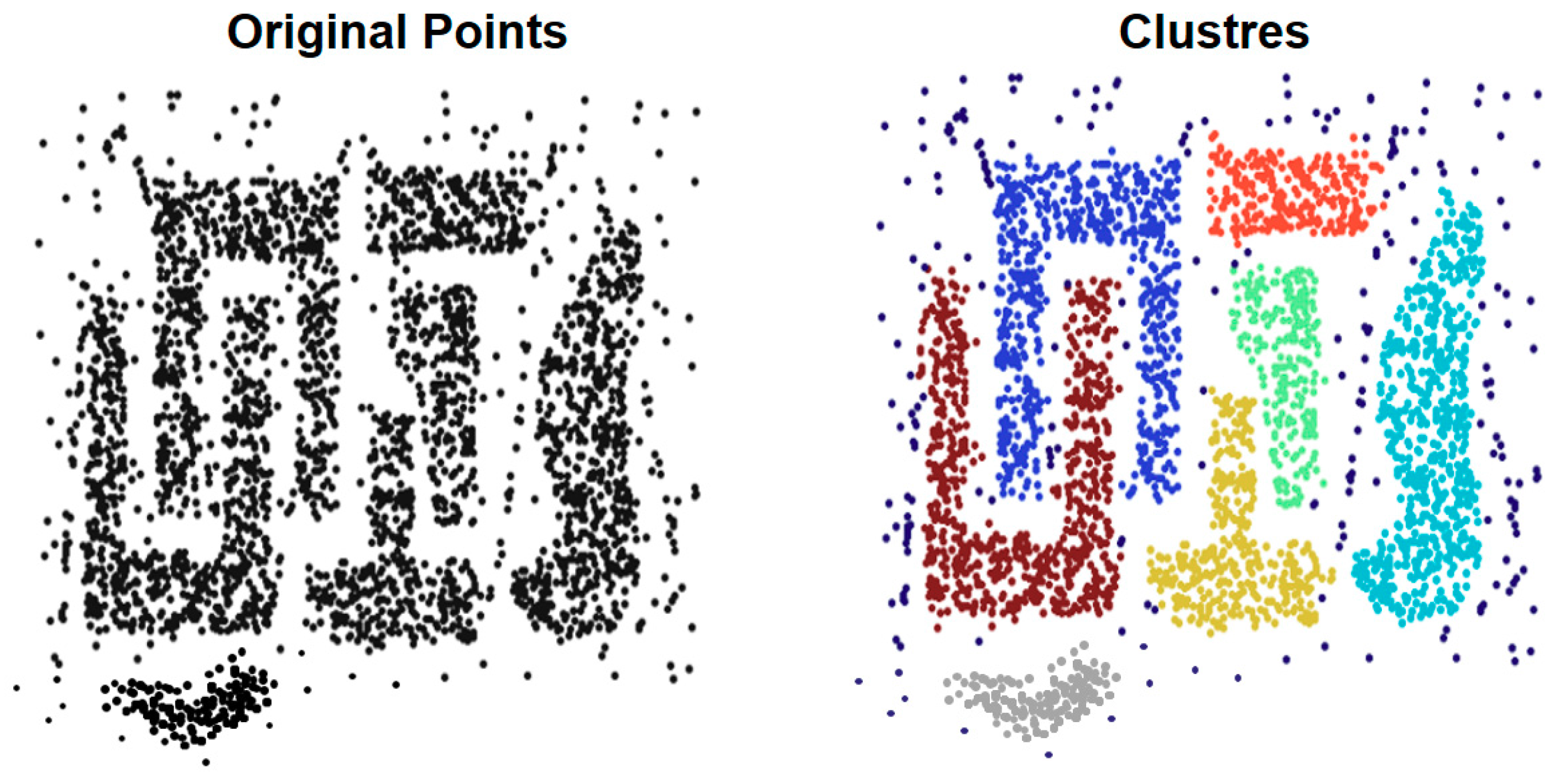
DBSCAN (Density-based spatial clustering of applications with noise) was developed based on the density concept [7]. Twenty years after the introduction, the algorithm has become quite popular due to its simple concept and the relative ease of implementation. An important advantage of the algorithm is the ability to handle clusters of different shapes and sizes and noisy data, as shown in Figure 1. The DBSCAN algorithm can identify clusters in large spatial data sets by analyzing the local density of database elements using only one input parameter. Furthermore, the user receives a suggestion on which parameter value would be suitable. Therefore, minimal knowledge of the domain is required. The DBSCAN can also determine which information should be classified as noise or outliers.
The key concept of DBSCAN algorithm will be elaborated in Figure 2 and it is defined as following:
Definition 1.
Eps neighborhood: For the given data set D, , we call the neighborhood which uses object p as the center, Eps as the radius as the Eps neighborhood of the object p.
Definition 2.
Density threshold Minpts: For the given data set D, , the density threshold which make the object p as the core object is called as density threshold Minpts.
Definition 3.
Core object: For the given data set D, , and are in the Eps neighborhood of the object p. If the n is bigger than the density threshold Minpts, that means the number of object in the Eps neighborhood of object p is bigger than density threshold Minpts, then the object p is the core object.
Definition 4.
Directly density-reachable: For the given data set D, , q is in the Eps neighborhood of the object p and object p is the core object. Then we called q is directly density-reachable from object p.
Definition 5.
Density-reachable: For the given data set D, , . For the object , if is directly density-reachable from object about Eps and Minpts. Then we called the object q is density-reachable from object p about Eps and Minpts.
Definition 6.
Density-connected: For the given data set D, . If , object p and q are density-reachable from object o about Eps and Minpts. Then object p and q are density-connected about Eps and Minpts.
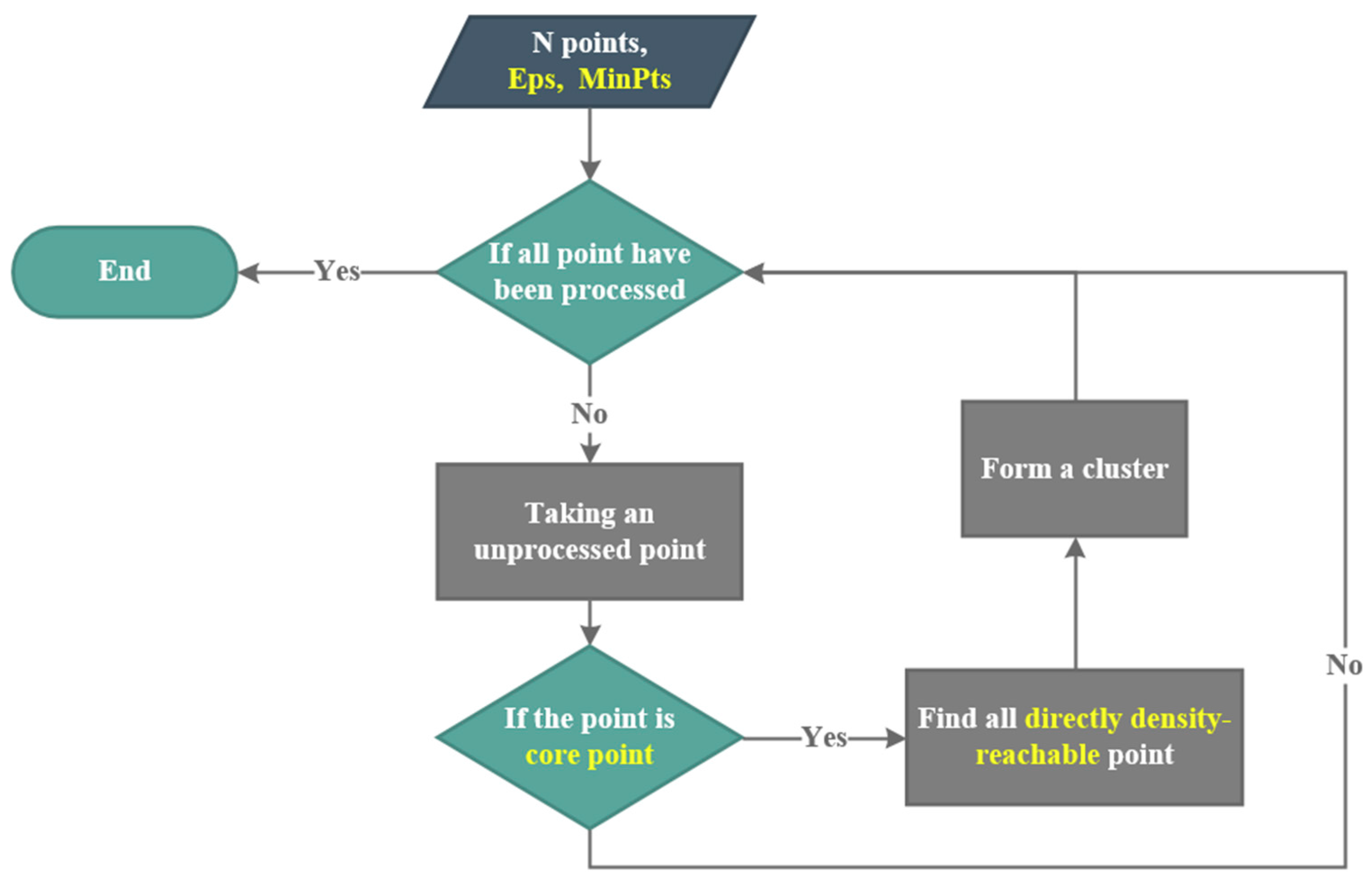
Assume that the input parameter is the Eps and Minpts, DBSCAN algorithm is described below:
- Inputting the data set and choosing an arbitrary data point x. Checking the Eps neighborhood of the data point x.
- If the point x is the core object and has not been divided by a certain class, then finding all density-reachable object from data point x. Finally, we can get a neighborhood include point x.
- If the point x is not the core object, then taking the point as the noise.
- Turn to the first step, repeating the algorithm until all the point in the data set has been handled.
2.2. Density-Based 4D Clustering Algorithm: ST-DBSCAN
Spatial-temporal density-based clustering is the extension of the spatial density clustering method, which uses density as the measurement of similarity between the objects and takes the spatial-temporal cluster as a series of high-density connectivity regions segmented by low-density area (noise). Reference [9] proposes the ST-DBSCAN, on the basis of the DBSCAN [10] algorithm, which accounts for the time dimension. Reference [11] presents an analogous spatial-temporal clustering algorithm. However, unlike the ST-DBSCAN, their method can utilize the non-spatial attribution similarity. The main extension of the ST-DBSCAN algorithm is using the spatial-temporal neighboring areas method, which is similar to the space-time scan statistics method [12], to estimate the spatiotemporal entity density. Figure 5 illustrates the concept of the spatial-temporal neighboring area. The spatial-temporal neighboring area of the spatio-temporal entity is defined as a cylinder which has a radius of R and a height of . The density of is the entity number in the cylinder spatial-temporal neighboring area. Other definitions of the ST-DBSCAN are the same as the DBSCAN algorithm, such as the concept of directly density-reachable, density-reachable and density-connected [10]. The basic workflow of the ST-DBSCAN is the same as the DBSCAN algorithm seen in Figure 4. Due to utilizing the time dimension, the ST-DBSCAN algorithm requires three parameters: space radius R, time window and density threshold MinPts. First, two parameters are used to determine the spatial-temporal neighboring area. The ST-DBSCAN algorithm inherits the fine properties of the DBSCAN algorithm, such as the adaptation to arbitrarily shaped spatial-temporal clusters, non-data distribution presupposition and noise resistant ability. The series of fine properties is the reason for choosing the ST-DBSCAN algorithm to perform the spatial-temporal clustering. Moreover, [9,11] gives the empirical parameters determination method for the three ST-DBSCAN parameters. It includes: sorting the k-nearest neighbor graph method to determine the spatial radius R and time window , taking the as MinPts where the N is the spatial-temporal entity number.
2.3. Automatic Fracture Plane Identification Implementation
Once accurate clustering results are determined, we will perform the single fracture plane fitting. Based on the hypothesis of the same crack belonging to the same class, we can obtain an accurate single fracture plane. This methodology is summarized below:
- (1)
- Obtain high signal-to-noise ratio seismic data
- (2)
- Obtain high precision micro earthquake location results
- (3)
- Obtain the classification results using the clustering analysis algorithm we have proposed.
- (4)
- Use the least squares fitting method to obtain an accurate single fracture plane.
Above, we achieve the automatic fracture surface recognition method theory. We proposed this method based entirely on space-time data dependencies, without human intervention and with the characteristics of noise suppression.
3. Acoustic Emission Verified Experiment
After we proposed our automatic fracture plane recognition algorithm, a verified experiment was needed to test the effectiveness of our method. For hydraulic fracturing construction, both the generation of micro-seismic events and fracture plane recognition lack the ability to obtain underground crushing information. Therefore, we select the rock physical dimension as a testing tool. Through the rock physics experiment, we can use CT (Computed Tomography) scan results of the sample to compare with the fracture plane recognition results. Accordingly, if the CT scan results are similar to the algorithm analysis results, the effectiveness of our fracture plane recognition algorithm can be verified.
The rock samples of this experiment are the Lower Silurian Longmaxi Shale in the Sichuan Basin. The Sichuan Basin is a Mesozoic-Cenozoic basin with complex tectonics. The Triassic formation composed of marine deposits is an important potential resource and reservoir. Shale is an important part of hydrocarbon source rocks in the Sichuan Basin with the high gas generating ability and large distribution area. It is the primary contributor of natural gas resources in the Sichuan Basin. Figure 6 shows one of the cores (100 mm × 200 mm) drilled from an outcrop at Jiaoshiba, Chongqing City. Figure 7 is the original rock core CT scan image. Through the CT scan, we observe that the rock core has a primary fracture development along the bedding plane of the axial center location, seen in Figure 7. Using the characteristics of the primary fracture development as the main purpose of the experiment, we take the original cracks as the fluid injection channel to simulate the fluid injection process using horizontal well fracturing in the field exploration of the hydraulic fracturing process. To monitor the acoustic emission signals generated by water fracturing, we lay 20 piezoelectric sensors (pzt) on the surface of the core. The specimen was sealed by silicone coat to isolate the test sample from the confining oil. The core preparation process is shown in Figure 8.
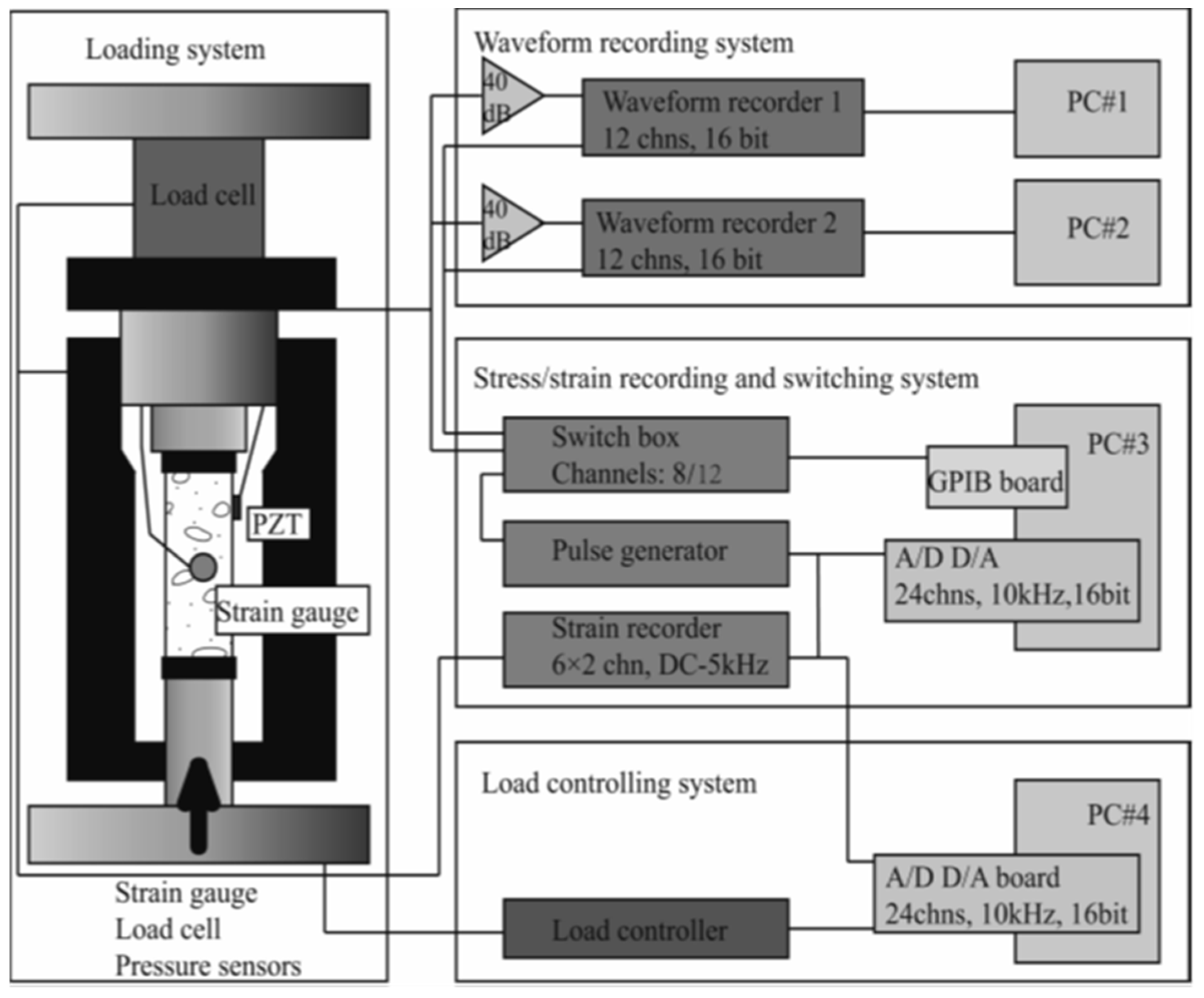
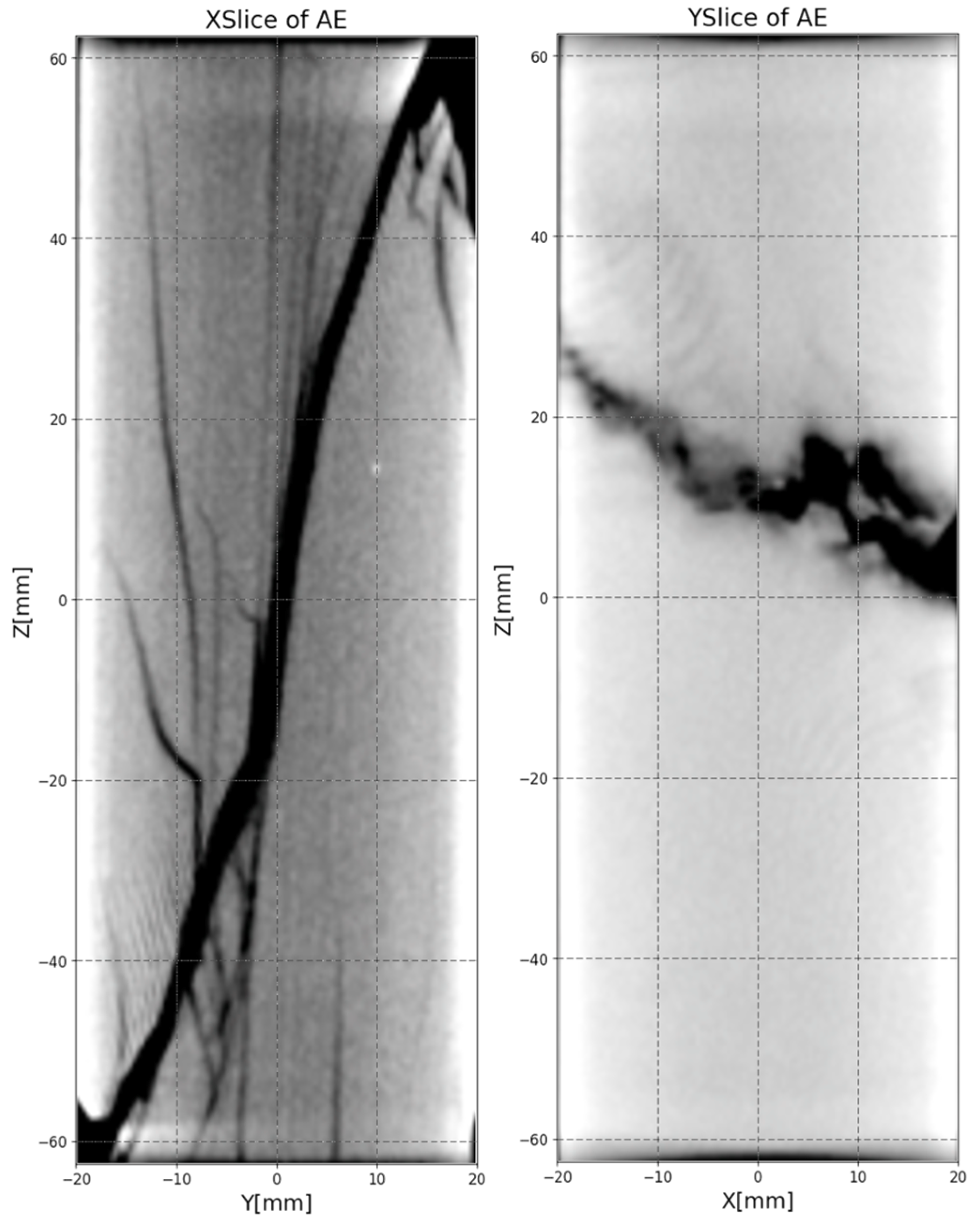
This experiment is performed on a triaxial compression apparatus and a multi-channel acoustic emission waveform acquisition system at the Japan Industrial Technology Research Institute, as seen in Figure 9. The system primarily includes a loading system, the acoustic emission counts and waveform acquisition system and a stress and strain monitoring system composed of three parts. The loading system includes axial compression loading and confining pressure loading. The pressure vessel is placed in the uniaxial compression experiment of 2000 tons. Confining oil is pumped through the pipeline to exert confining pressure on the rock pressure vessel. The acoustic emission waveform acquisition system is composed of the amplifier and two sets of 12-channel full waveform high-speed analog-to-digital conversion cards. The received probe signal passes to the acoustic emission waveform acquisition card after the 40 dB amplifier. The dead time of the acquisition card is less than 200 μs. Therefore, we can record the full waveform data of almost all detected acoustic signal emission events to evaluate the rock damage process in detail. Experiments after the failure events analyze samples using X-ray CT scanning and the internal analysis of the rock fracture surface shape from the CT scan is shown in Figure 10.
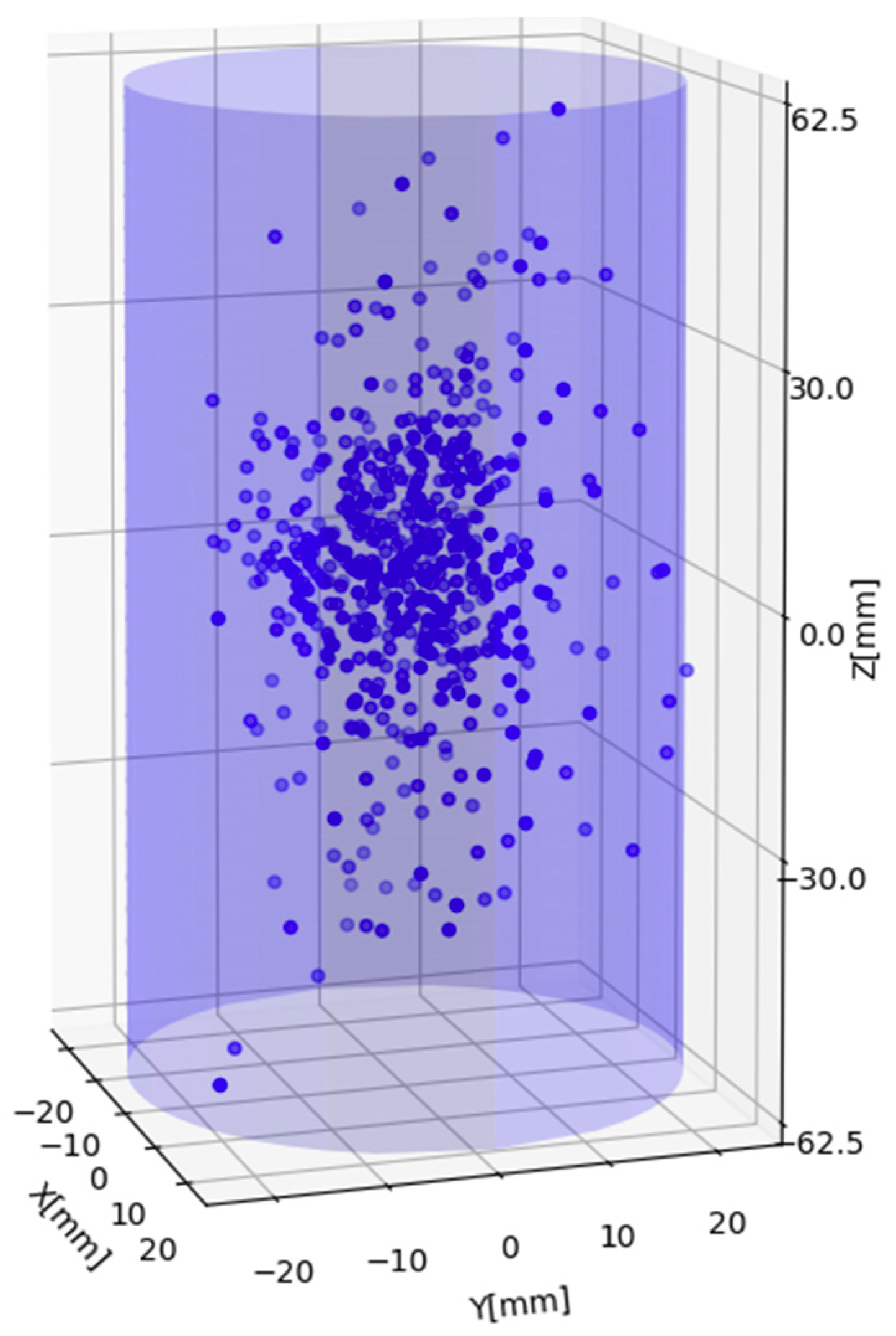
After the experiment, we perform an X-ray CT scan of broken rock samples to analyze the internal fracture surface morphology of the rock. After the scanning analysis, we use the 20-channel full waveform acoustic emission data of the pzt sensor installed on the core to obtain the acoustic emission events positioning results, as shown in Figure 11.
Once we obtain the precise positioning of micro-seismic events and rock fracturing fault CT scans results, we can start the validation of our automatic fault plane recognition algorithm.
4. Parameter Detection and Sensitivity Analysis
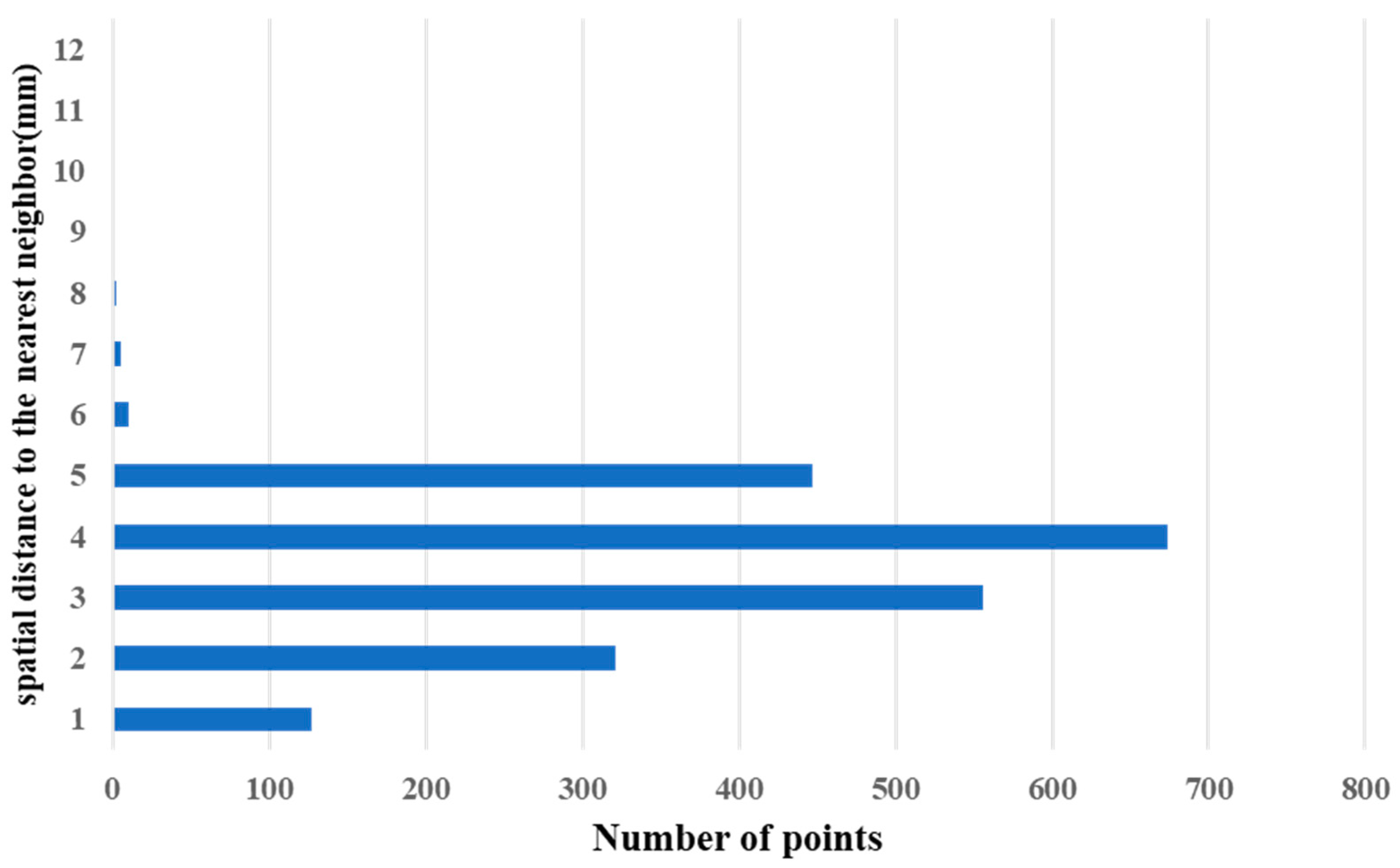
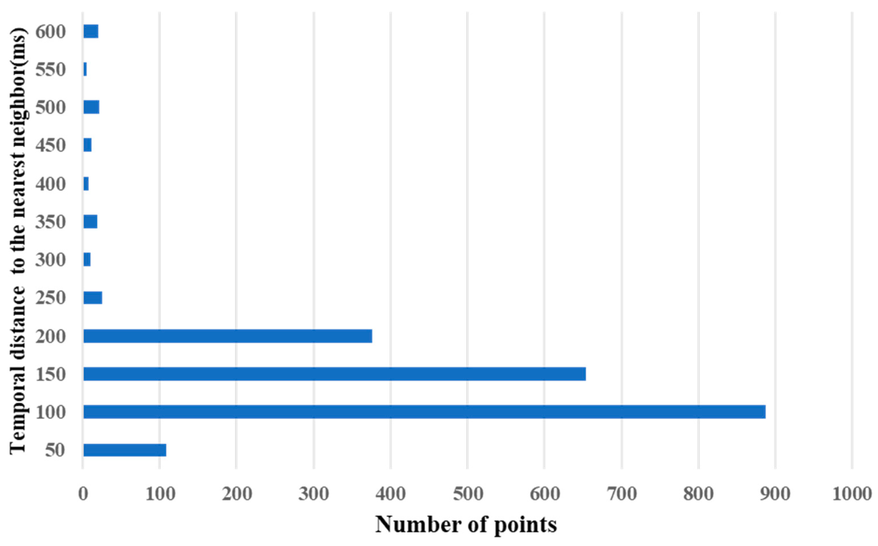
The algorithm of space-time clustering that we used requires three parameters: two Eps parameters, which specify how close the points should be to each other to be considered a part of a cluster in the time and space dimensions and one MinPts parameter, which specifies how many neighbors a point should have to be included into a cluster. Reference [5] provides the empirical parameter determination method for the three ST-DBSCAN parameters. The method includes: sorting the k-nearest neighbor graph method to determine the spatial radius R and the time window, taking the ln(N) as MinPts where N is the spatial-temporal entity number. Because we have 2143 validity events, the MinPts is equal to 7. For the two Eps parameters, we need to calculate the time and space distance from each point to its nearest neighbor within the same partition and find the mutations in the histogram value. This distance will not be accurate for a small fraction of points. However, this inaccuracy does not significantly affect the overall distribution of the distances. The result for estimating the two Eps parameters is shown in Figure 12 and Figure 13. It indicates that the vast majority of points lie within five units from their nearest neighbor in the space dimension and four units in the time dimension. Therefore 5 mm and 200 ms may be reasonable estimates for the space epsilon parameter and time epsilon parameter.
The ST-DBSCAN algorithm is dependent on parameter selection. Different parameters values will result in different results. Therefore, the results of fracture plane identification may depend on these parameters. Although we have adopted the most widely used empirical formula for parameters calculation, these formulas also have the data dependency and applicability issues. Accordingly, we introduced the parameters sensitivity analysis to evaluate the impacts of varying ST-DBSCAN parameters on fracture plane identification issues. In the sensitivity analysis section, we will follow the method proposed by [11] and conduct a limited scope sensitivity analysis using a series of parameter values for the ST-DBSCAN algorithm.
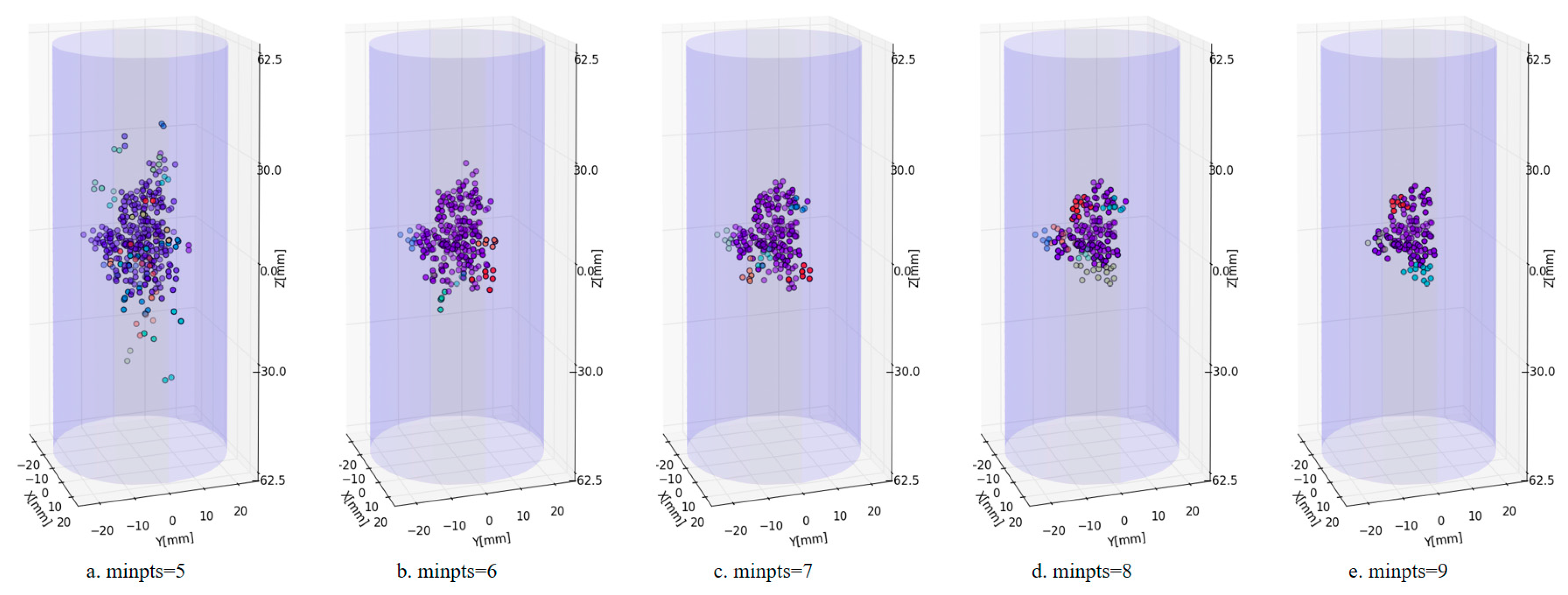
To evaluate the influence of different MinPts values, we set the fixed Eps (Eps_t, Eps_s) by the given empirical formula. The MinPts was altered from 5 to 9. According to the different MinPts values, we draw the calculated clusters results as shown in Figure 14. We can find that a low MinPts means it will build more clusters from noise, so do not choose it too small. At the same time, we find that when the value of MinPts is increasing, the algorithm ignored many small classes and fewer classes are preserved. For the fracture plane identification problem, we know the prior information that there must be the main crack and there must have amount of small crack. Therefore, we require ensuring the selection of MinPts does not produce too many clusters and does not make too centralized clustering results. By comparison the different MinPts selection results, we can find that the MinPts selected by the empirical formula satisfies the parameter selection criteria. The Minpts obtained through the empirical formula is suitable for our fracture plane identification problem.
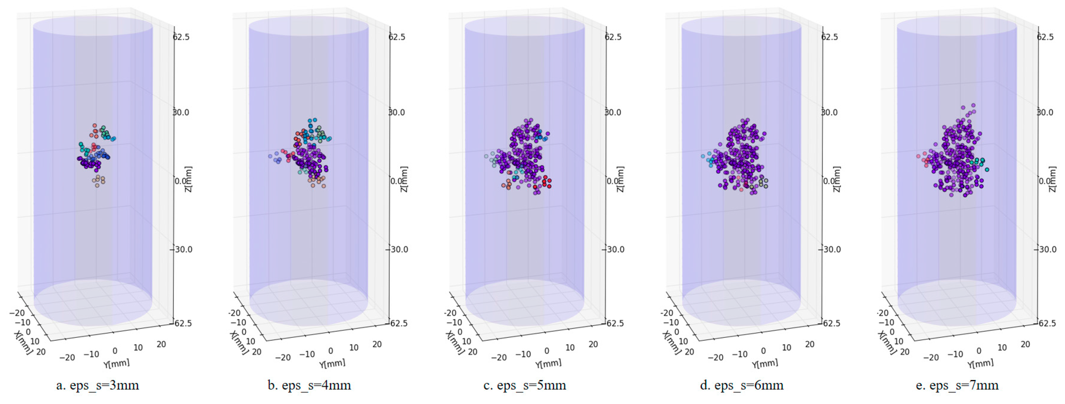
For the two Eps (Eps_s, Eps_t), we adopted the same analysis method as above and fixed other parameters to analyze the influence of different Eps (Eps_s, Eps_t) on the clustering results. For the Eps_s parameter, we set the fixed Eps_t, Minpts by the given empirical formula. The Eps_s was altered from 3 mm to 7 mm. According to the different Eps_s values, we draw the calculated clusters results as shown in Figure 15. For the Eps_t parameter, we set the fixed Eps_s, Minpts by the given empirical formula. The Eps_t was altered from 50 ms to 250 ms. According to the different Eps_t values, we draw the calculated clusters results as shown in Figure 16. By comparison the different Eps (Eps_s, Eps_t) parameters selection results, we can find that the Eps selected by the empirical formula satisfies the parameter selection criteria. The Eps obtained through the empirical formula is suitable for our fracture plane identification problem.
5. Results
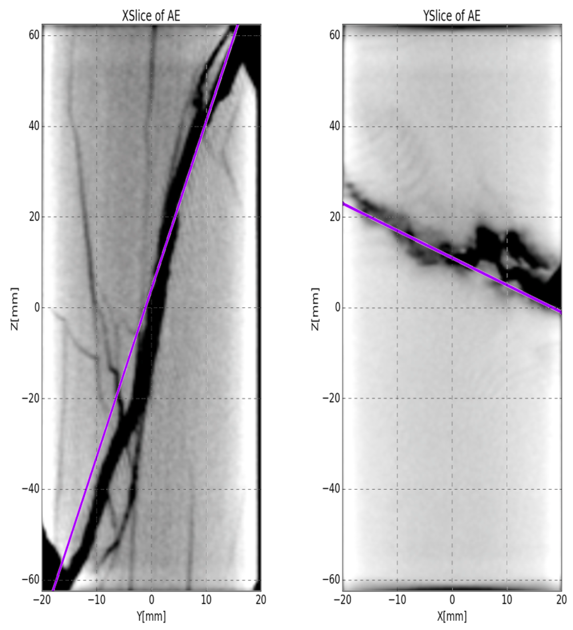
Based on the choice of algorithm parameters during the acoustic emission data clustering analysis, the result is shown in Figure 17. Through the clustering analysis, six classes and the primary and secondary cracks were identified and the noise points were largely removed. We extract the primary information shown in Figure 18a and use these points for surface fitting to obtain the primary fracture plane recognition results, shown in Figure 18b. The fracture plane fitting result shown in Figure 18b is obtained using the least squares regression method. In addition, the results are compared to the actual fractured rock sample. Through sifting sort, we choose the fracture surface which intersects the outer surface of the rock sample. Drawing the outer surface intersection line, the results are shown in Figure 18b. After determining the intersection information shown in Figure 18b, it is compared to the actual sample. To achieve more intuitive results, the CT scan and the plane fitting results are overlapped for a comparison display.
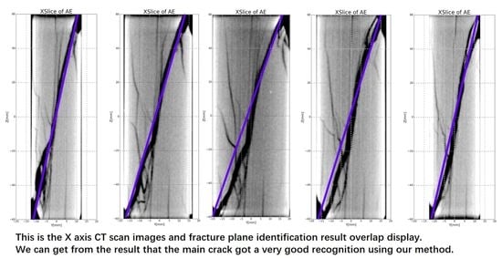
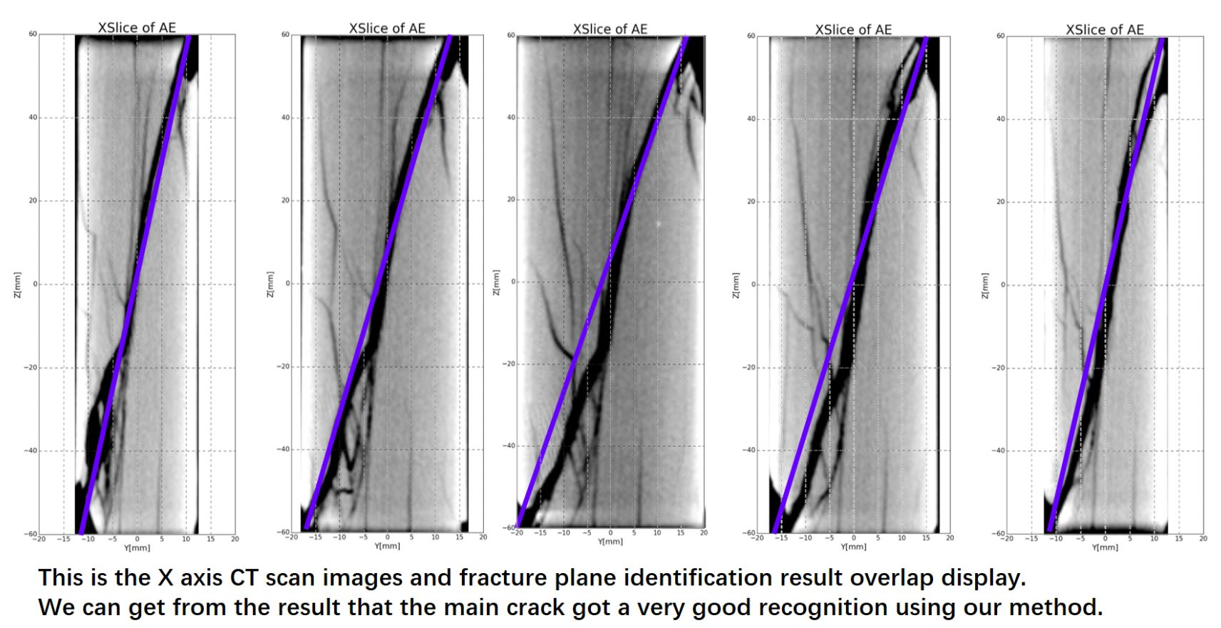
Figure 19 reflect the rupture intersection line between our algorithm results and the actual rock sample. Through the comparison of Figure 19, the main fracture information is significantly reduced and the broken side seam also has an acceptable correspondence. These results further illustrate the feasibility of our algorithm.
6. Discussion and Conclusions
We proposed a dynamic fracture plane identification algorithm for micro-seismic data. The primary advantage of the proposed workflow is the utilization of temporal and spatial attribute constraints, which make it an automated method. In addition, it has anti-noise properties, which are beneficial for the micro-seismic environment. Through the example of a rock acoustic emission experiment, we validate this method. The primary fracture in the rock can be identified automatically and the result is acceptable. The overall crack fracture trend of the rock core will be determined using the proposed algorithm. Although our method is verified by the experimental data of rock physics, there are still many limitations to our approach. First, our method is dependent on the selection of core parameters. Whether the parameters of different lithology rocks can be selected by the same empirical formula. This issue still needs further discussion. Meanwhile, our method has quite good identification result for the apparent main fracture. However, the current algorithm cannot get a credible result for the small and secondary fractures due to the limited acoustic emission data. The follow-up research needs to mine the geophysical properties of the acoustic emission data, such as the seismic moment tensor and the earthquake magnitude. Adding these attributes to the clustering algorithm will make the small and secondary fracture plane identification result more accurate and reliable.
In conclusion, rock physics experimental results show the effectiveness and robustness of our algorithm. Moreover, future research should incorporate focal mechanism attribute information into this method. All fractures in the same failure plane acoustic emission events are presumed to have the same focal mechanism properties. Determining the combination of the space-time attributes and prior knowledge of the fracturing mechanism will enable this method to explore more information extraction from the acoustic emission data.
Acknowledgments
The research was supported by the National Program on Key Basic Research Project of China (973 Program) for Young Scholars (Grant No. 2015CB258500) and funded by the National Science Foundation of China, Grant No. 41390455.
Author Contributions
Each author has contributed to the present paper. Yibo Wang conceived the idea and directed the experiments; Qingfeng Xue analyzed the data and wrote the paper; Xu Chang directed the experiments; Hongyu Zhai performed the experiments.
References
- Thornton, M.; Eisner, L. Uncertainty in Surface Microseismic Monitoring. In Proceedings of the SEG San Antonio 2011 Annual Meeting, San Antonio, TX, USA, 18–23 September 2011; pp. 1524–1528. [Google Scholar]
- Busetti, S.; Jiao, W.; Reches, Z. Geomechanics of hydrolic fracturing microseismicity: Part 1. Shear, hybrid, and tensile events. Am. Assoc. Pet. Geol. Bull. 2014, 98, 2439–2457. [Google Scholar] [CrossRef]
- Wenlong, D.; Changchun, X.; Kai, J.; Chao, L.; Weite, Z.; Liming, W. The research progress of shale fractures. Adv. Earth Sci. 2011, 2, 3. [Google Scholar]
- Yu, Z.; Lai, F.; Xu, L.; Liu, L.; Yu, T.; Chen, J.; Zhu, Y. Study on fracture identification of shale reservoir based on electrical imaging logging. In IOP Conference Series: Earth and Environmental Science; IOP Publishing: Bristol, UK, 2017; Volume 64, p. 12041. [Google Scholar]
- King, G.E. Thirty years of gas shale fracturing: What have we learned? In SPE Annual Technical Conference and Exhibition; Society of Petroleum Engineers: Richardson, TX, USA, 2010. [Google Scholar]
- Eshiet, K.I.; Sheng, Y.; Ye, J. Microscopic modelling of the hydraulic fracturing process. Environ. Earth Sci. 2013, 68, 1169–1186. [Google Scholar] [CrossRef]
- Fayyad, U.; Piatetsky-Shapiro, G.; Smyth, P. From data mining to knowledge discovery in databases. AI Mag. 1996, 17, 37. [Google Scholar] [CrossRef]
- Alhanjouri, M.A.; Ahmed, R.D. New density-based clustering technique: GMDBSCAN-UR. Int. J. Adv. Res. Comput. Sci. 2012, 3, 1–9. [Google Scholar]
- Wang, M.; Wang, A.; Li, A. Mining spatial-temporal clusters from geo-databases. In Advanced Data Mining and Applications; Springer: New York, NY, USA, 2006; pp. 263–270. [Google Scholar]
- Ester, M.; Kriegel, H.-P.; Sander, J.; Xu, X. A density-based algorithm for discovering clusters in large spatial databases with noise. In Proceedings of the Second International Conference on Knowledge Discovery and Data Mining, Portland, OR, USA, 2–4 August, 1996. [Google Scholar]
- Birant, D.; Kut, A. ST-DBSCAN: An algorithm for clustering spatial–temporal data. Data Knowl. Eng. 2007, 60, 208–221. [Google Scholar] [CrossRef]
- Tango, T. Space-Time Scan Statistics. In Statistical Methods for Disease Clustering; Springer: New York, NY, USA, 2010; pp. 211–233. [Google Scholar]
- Li, X.Y.; Lei, X.L.; Li, Q.; Cui, Y.X. Characteristics of acoustic emission during deformation and failure of typical reservoir rocks under triaxial compression: An example of Sinian dolomite and shale in the Sichuan Basin. Chin. J. Geophys. Chin. Ed. 2015, 58, 982–992. [Google Scholar]
Figure 1.
This figure (modified from [8]) shows the functionality of DBSCAN algorithm, after applying DBSCAN, the noises can be excluded and the points can be classified to clusters.
Figure 1.
This figure (modified from [8]) shows the functionality of DBSCAN algorithm, after applying DBSCAN, the noises can be excluded and the points can be classified to clusters.

Figure 2.
Key definitions used in DBSCAN approach. (a) Shows a cluster of points. The red point in (b) is a core object. The green point in (c) is a border point. In (d) all red points are density-reachable objects.
Figure 2.
Key definitions used in DBSCAN approach. (a) Shows a cluster of points. The red point in (b) is a core object. The green point in (c) is a border point. In (d) all red points are density-reachable objects.
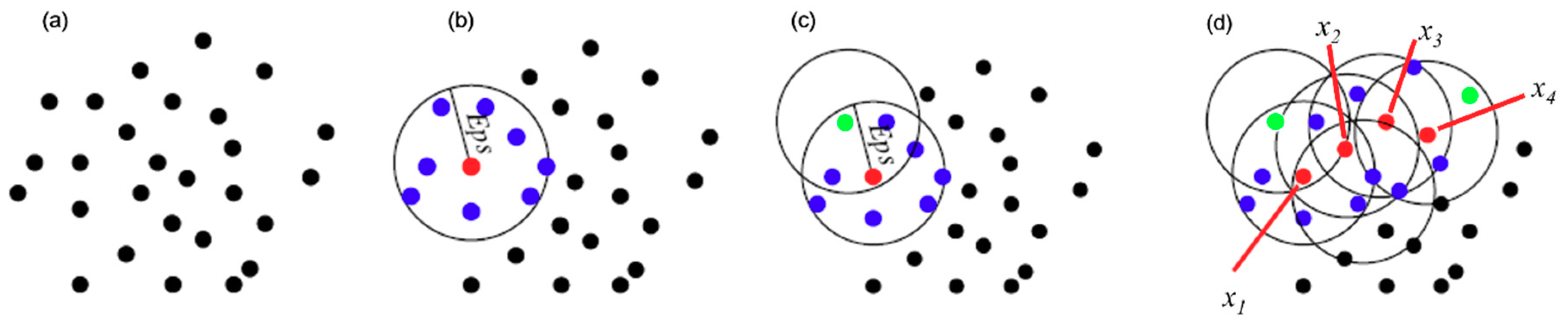
Figure 3.
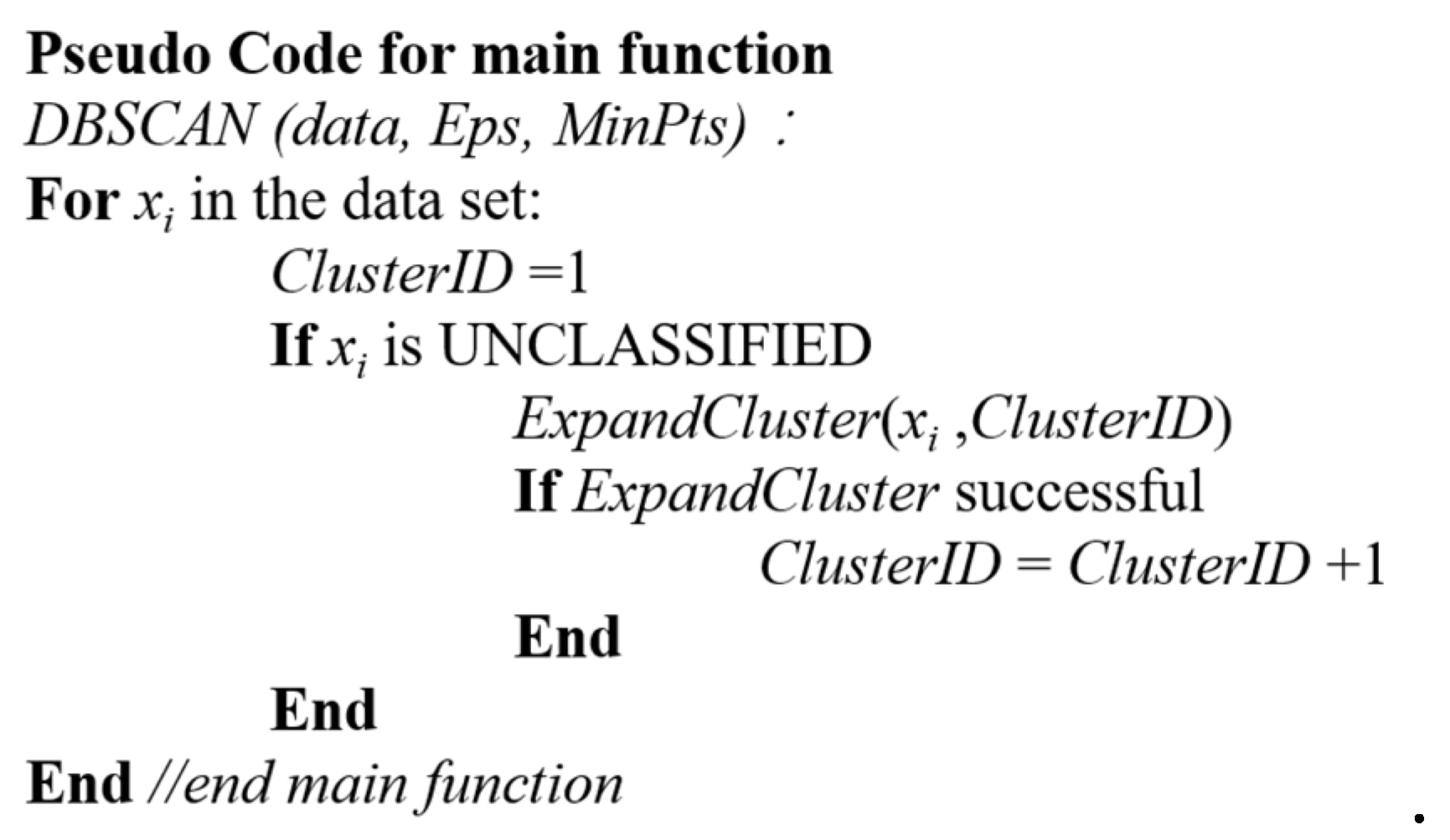
The pseudocode for the main function of the DBSCAN algorithm.

Figure 4.
The detailed algorithm processing workflow for the density based clustering algorithms.

Figure 5.
The spatial temporal neighboring region schematic diagram, after introducing time property. The space-time neighboring region in this figure means two-dimensional of space and one dimensional of time. The definition of the blue and red dots follows Figure 2.
Figure 5.
The spatial temporal neighboring region schematic diagram, after introducing time property. The space-time neighboring region in this figure means two-dimensional of space and one dimensional of time. The definition of the blue and red dots follows Figure 2.
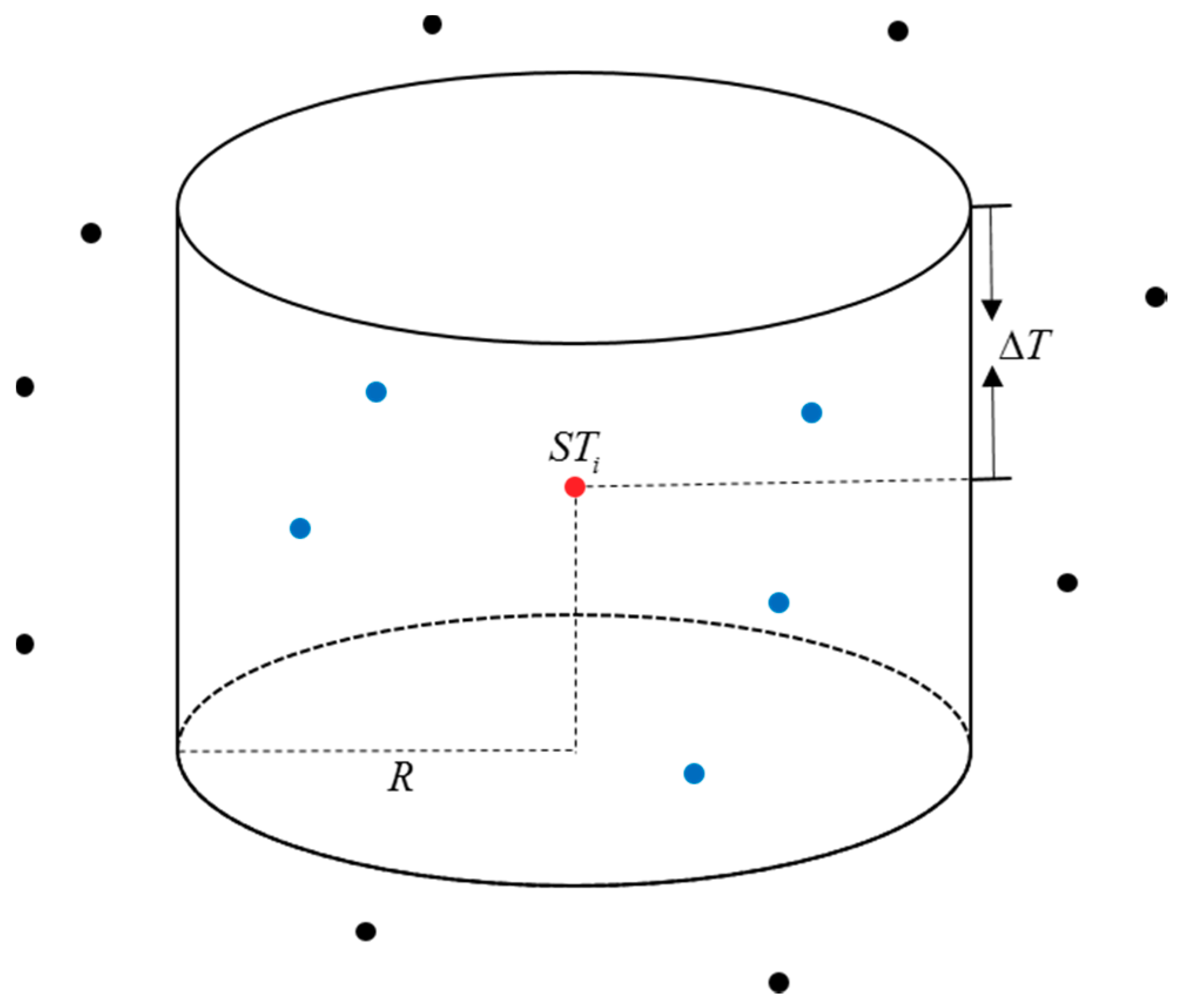
Figure 6.
Shale core from Jiaoshiba, Chongqing City.
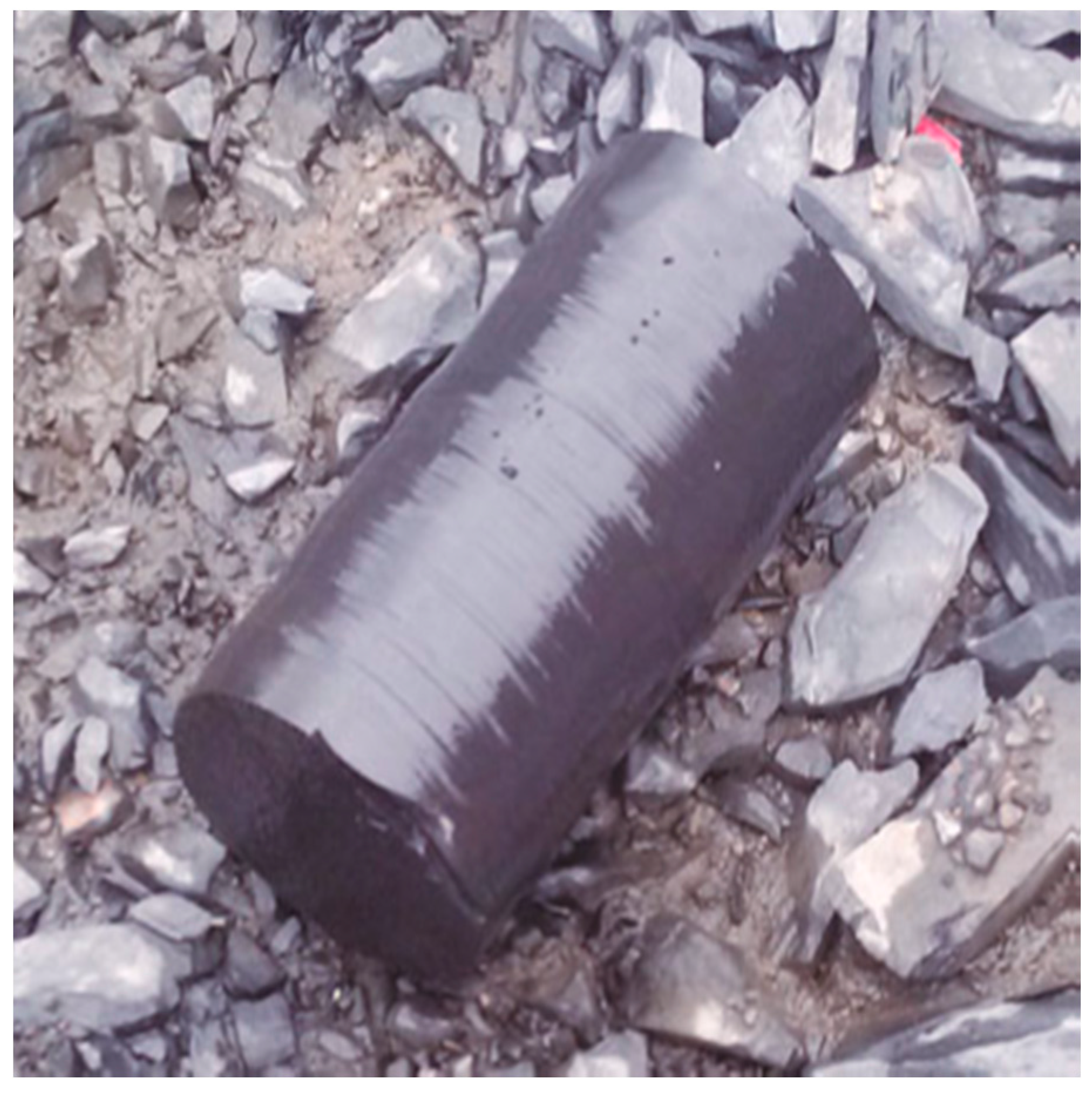
Figure 7.
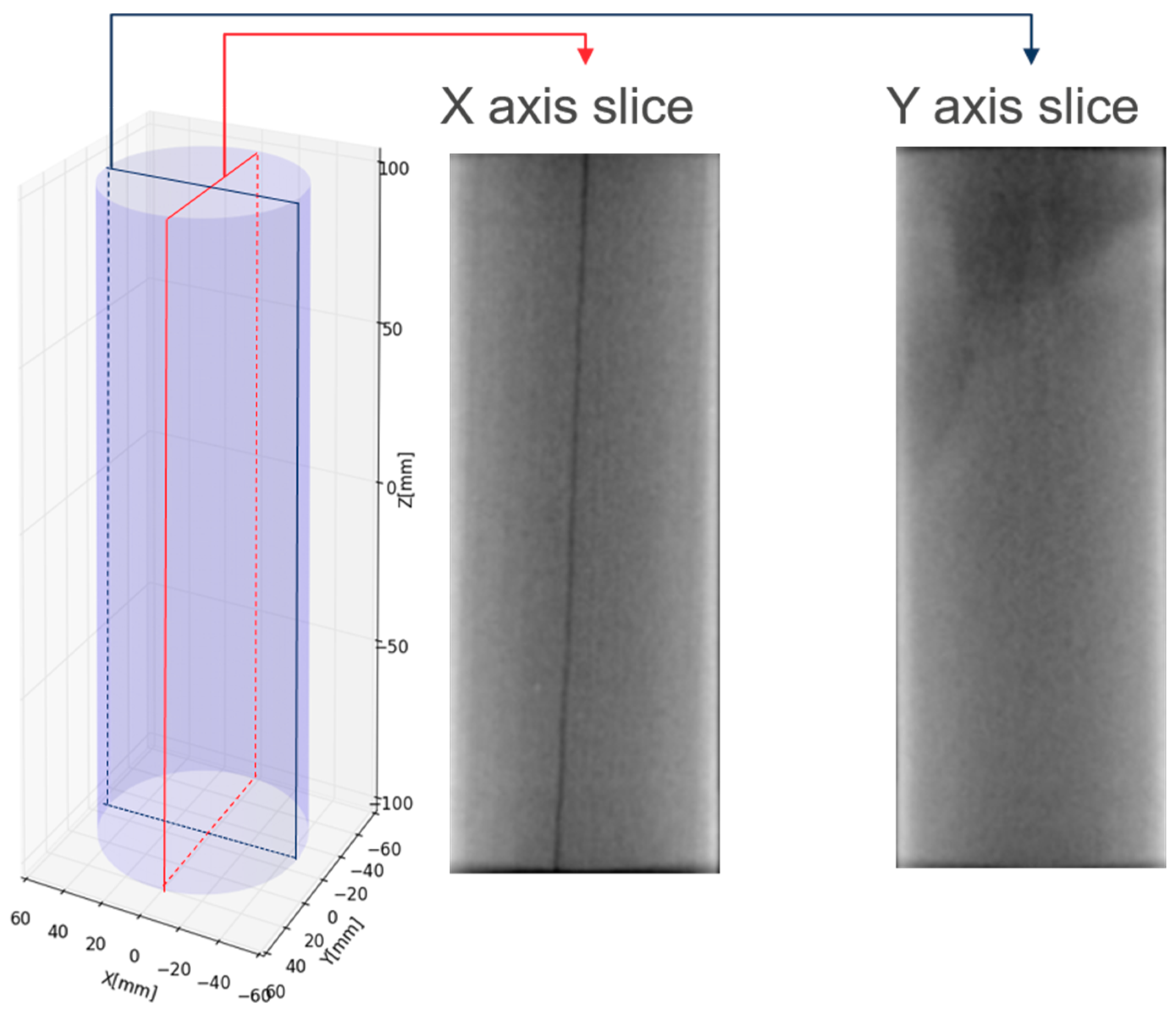
The original rock central position axial core CT scan images.

Figure 8.
The core preparation process. Figure (a) is the original experimental core, (b) is the core after the installation of PZT sensor, strain gauge and (c) is encapsulated core with adhesive.
Figure 8.
The core preparation process. Figure (a) is the original experimental core, (b) is the core after the installation of PZT sensor, strain gauge and (c) is encapsulated core with adhesive.
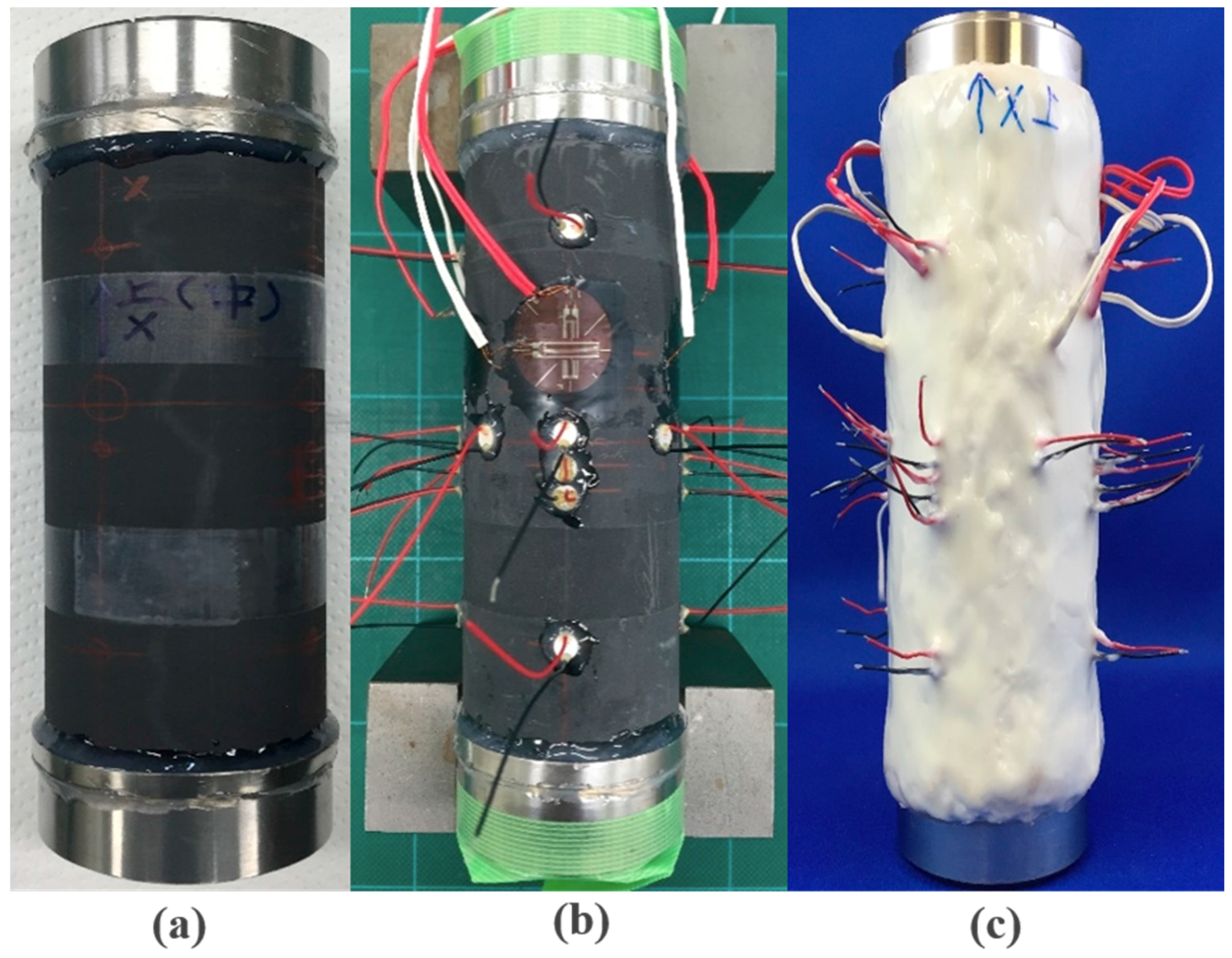
Figure 9.
The schematic diagram of the hydraulic fracturing experiment system [13].
Figure 9.
The schematic diagram of the hydraulic fracturing experiment system [13].

Figure 10.
The axle CT scan images in the X and Y direction after hydraulic fracturing.

Figure 11.
Acoustic emission events positioning results.

Figure 12.
Histogram for estimating spatial Eps parameter.

Figure 13.
Histogram for estimating temporal Eps parameter.

Figure 14.
Calculated clusters using different MinPts values and fixed Eps_s (5 mm), Eps_t (200 ms).
Figure 14.
Calculated clusters using different MinPts values and fixed Eps_s (5 mm), Eps_t (200 ms).

Figure 15.
Calculated clusters using different Eps_s values and fixed Eps_t (200 ms), MinPts (7).

Figure 16.
Calculated clusters using different Eps_t values and fixed Eps_s (5 mm), MinPts (7).
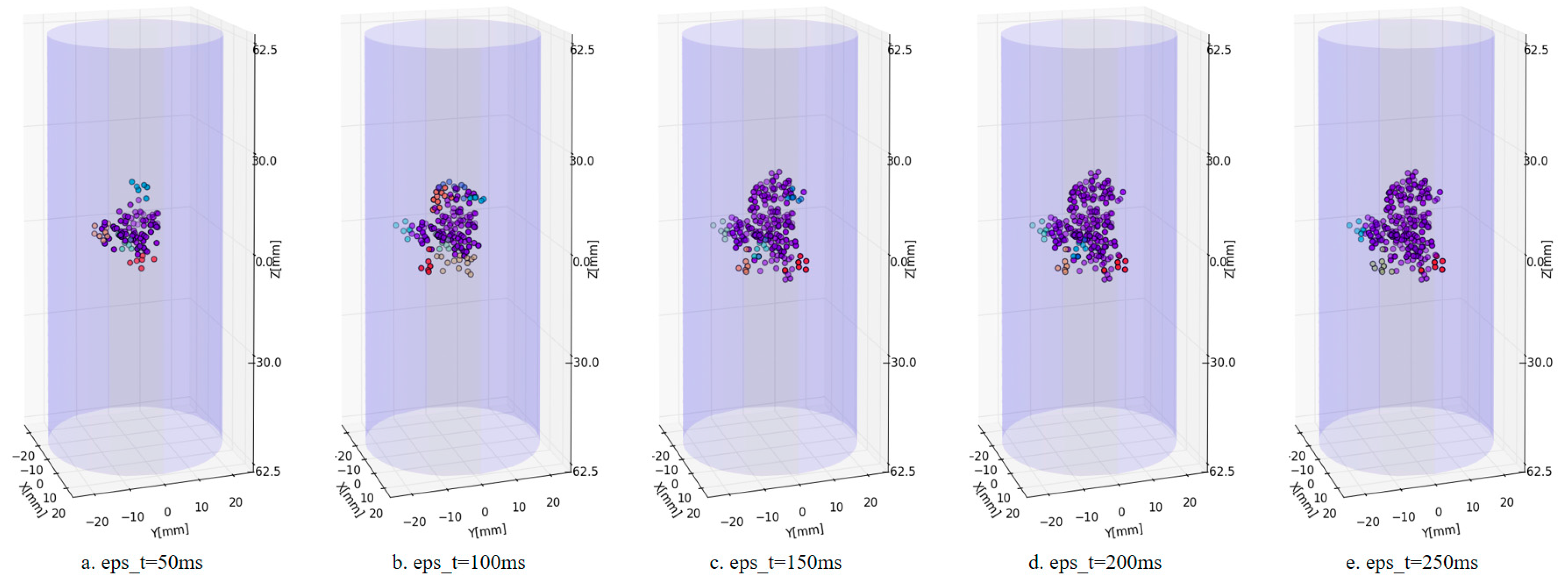
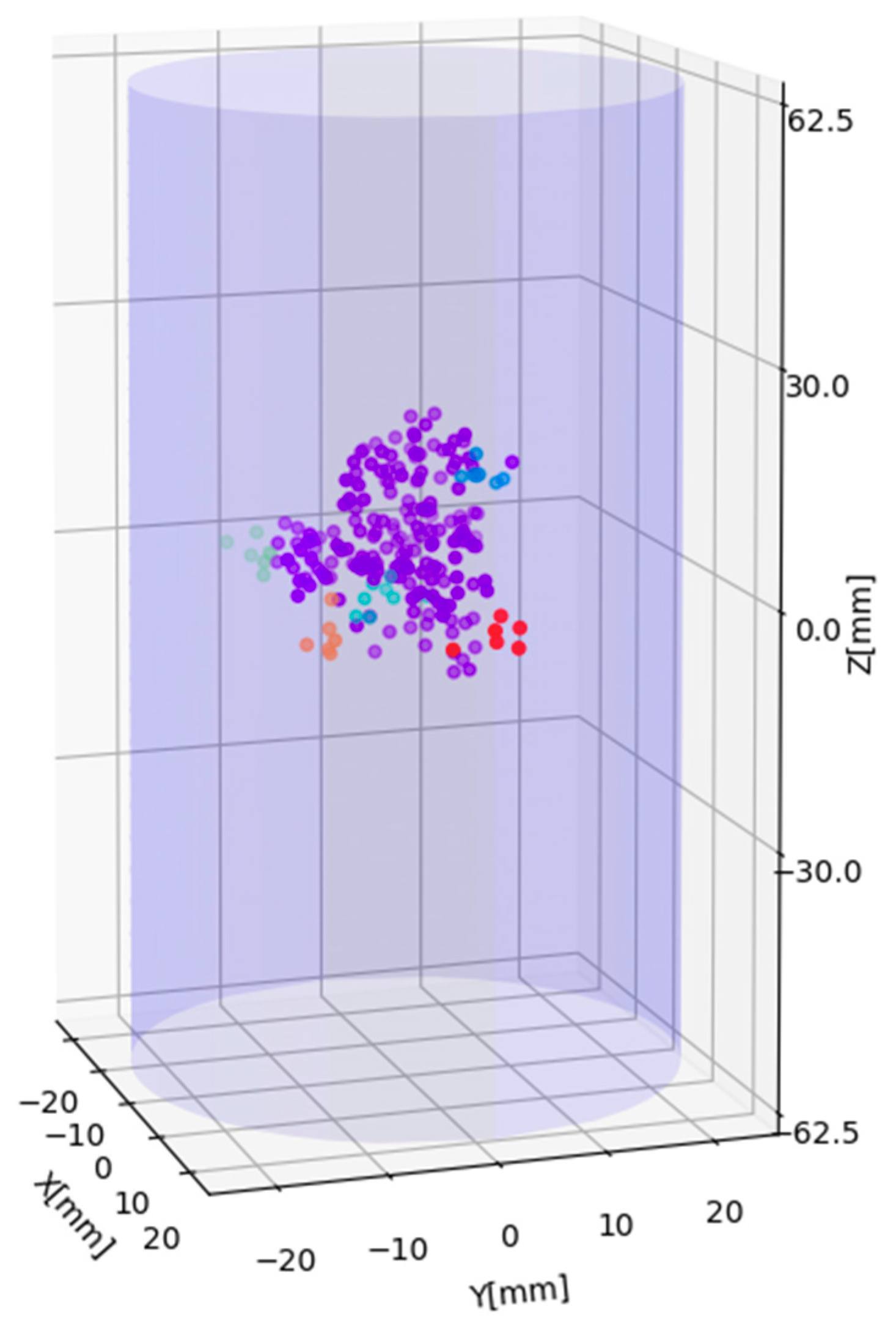
Figure 17.
ST-DBSCAN space-time clustering results of the acoustic emission events positioning results.
Figure 17.
ST-DBSCAN space-time clustering results of the acoustic emission events positioning results.

Figure 18.
This figure is about the main cluster. The extracted main cluster is shown in figure (a) and figure (b) is the main fracture plane recognition result.
Figure 18.
This figure is about the main cluster. The extracted main cluster is shown in figure (a) and figure (b) is the main fracture plane recognition result.
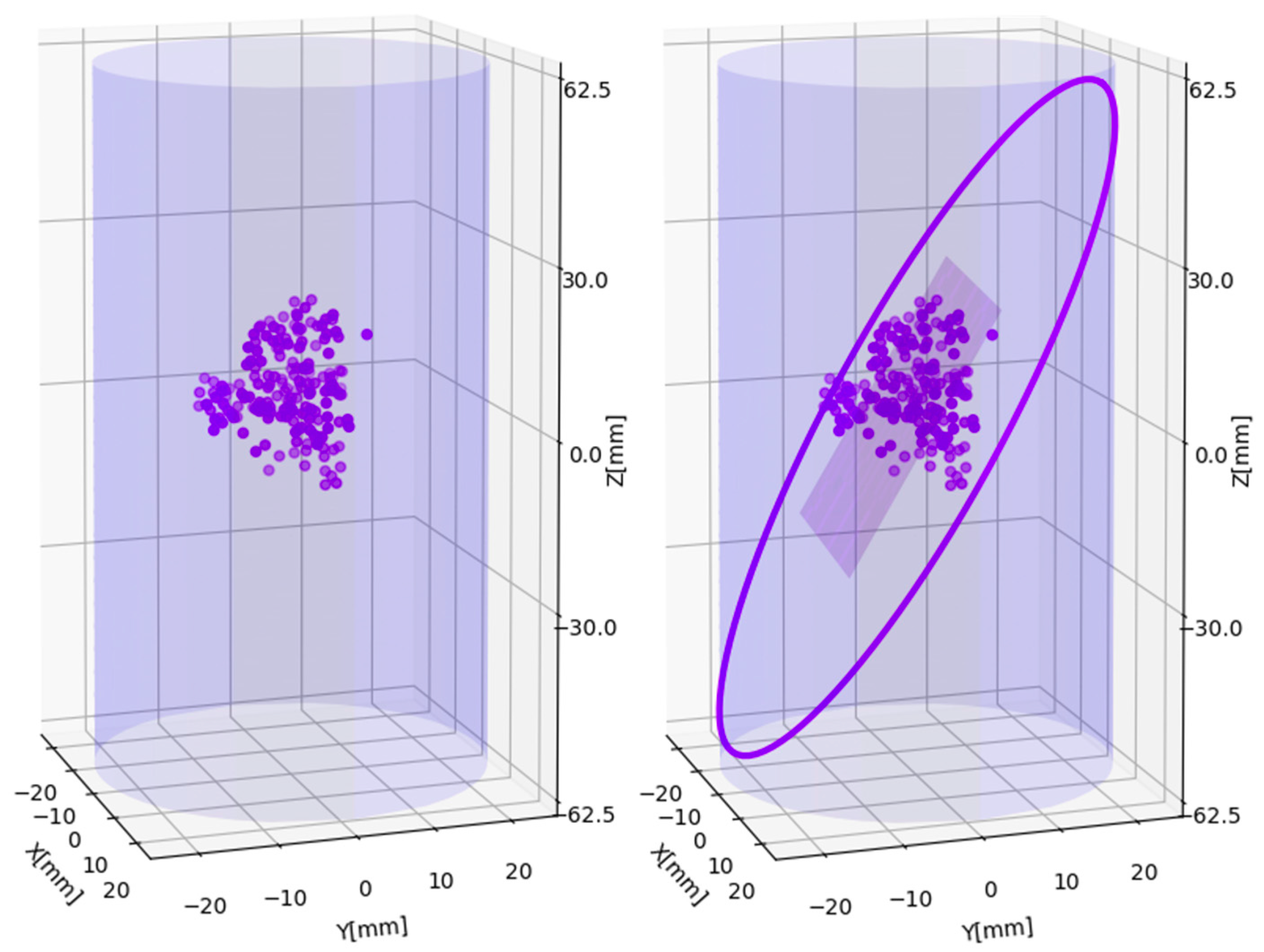
Figure 19.
This figure is the X and Y axis CT scan images and fracture plane identification result overlap display.
Figure 19.
This figure is the X and Y axis CT scan images and fracture plane identification result overlap display.
© 2018 by the authors. Licensee MDPI, Basel, Switzerland. This article is an open access article distributed under the terms and conditions of the Creative Commons Attribution (CC BY) license (http://creativecommons.org/licenses/by/4.0/).
Share and Cite
MDPI and ACS Style
Xue, Q.; Wang, Y.; Zhai, H.; Chang, X. Automatic Identification of Fractures Using a Density-Based Clustering Algorithm with Time-Spatial Constraints. Energies 2018, 11, 563. https://doi.org/10.3390/en11030563
AMA Style
Xue Q, Wang Y, Zhai H, Chang X. Automatic Identification of Fractures Using a Density-Based Clustering Algorithm with Time-Spatial Constraints. Energies. 2018; 11(3):563. https://doi.org/10.3390/en11030563
Chicago/Turabian StyleXue, Qingfeng, Yibo Wang, Hongyu Zhai, and Xu Chang. 2018. "Automatic Identification of Fractures Using a Density-Based Clustering Algorithm with Time-Spatial Constraints" Energies 11, no. 3: 563. https://doi.org/10.3390/en11030563
Note that from the first issue of 2016, this journal uses article numbers instead of page numbers. See further details here.