Air Release and Cavitation Modeling with a Lumped Parameter Approach Based on the Rayleigh–Plesset Equation: The Case of an External Gear Pump


1
Department of Mechanical and Nuclear Engineering, Pennsylvania State University, University Park, PA 16802, USA
2
Department of Mechanical Engineering, Purdue University, West Lafayette, IN 47907, USA
*
Author to whom correspondence should be addressed.
Energies 2018, 11(12), 3472; https://doi.org/10.3390/en11123472
Submission received: 2 November 2018
/
Revised: 4 December 2018
/
Accepted: 5 December 2018
/
Published: 12 December 2018
(This article belongs to the Special Issue Energy Efficiency and Controllability of Fluid Power Systems 2018)
Abstract
:In this paper, a novel approach for the simulation of cavitation and aeration in hydraulic systems using the lumped parameter method is presented. The presented approach called the Hybrid Rayleigh–Plesset Equation model is derived from the Rayleigh–Plesset Equation representative of bubble dynamics and overcomes several shortcomings present in existing lumped parameter based cavitation modeling approaches. Models based on static approximations do not consider the non-equilibrium effects of phase change on the system and incorrectly predict the system dynamics. On the other hand, the existing dynamic cavitation modeling strategies account for the non-equilibrium effects of phase change but express the evolution of phases through approximations of the Rayleigh–Plesset Equation (such as exclusion of nonlinear interactions in bubble dynamics), which often lead to physically unrealistic time-scales of bubble growth or dissolution. This paper presents a dynamic model for cavitation which is capable of predicting cavitation in hydraulic systems while preserving the nonlinear dynamics arising from the Rayleigh–Plesset Equation. The derived model determines the evolution of phases in terms of physically realizable parameters such as the bubble radius and the nuclei density, which can be estimated or determined experimentally. The paper demonstrates the effectiveness of the derived modeling approach with the help of numerical simulations of an External Gear Machine. Results from the simulations employing the proposed model are compared with an existing dynamic cavitation modeling approach and validated with experimental results over a range of dynamic parameters.
1. Introduction
Cavitation and aeration commonly occur in the operation of many fluid power systems, in particular in hydraulic components that are subjected to pressures below saturation pressure. It is well known that bubbles generated due to cavitation as well as aeration have detrimental effects in fluid power systems. They are undesirable not only due to the mechanical damage and noise resulting from the implosion of bubbles but also because they negatively affect the volumetric ability of positive displacement machines. Such undesirable effects of cavitation and aeration on the performance of hydraulic system necessitates their modeling in the prediction of operation of fluid power systems.
In the modeling of fluid power systems, several approaches have been introduced to account for cavitation and aeration in fluids. Some of the early modeling approaches were developed for Computational Fluid Dynamics (CFD) simulation of flows, such as those by Merkle et al. [1], Zwart et al. [2], Schnerr and Sauer [3] among others. A detailed analysis of cavitation in fluid flow was done by Dabiri et al. [4,5,6] using direct CFD simulations. Merkle et al. [1] and Zwart et al. [2] developed models for sheet cavitation based on arbitrarily chosen velocity and time scales, whereas the model by Schnerr and Sauer [3] used approximations of the Rayleigh–Plesset Equation representative of bubble dynamics. Similar approaches involving approximations of the Rayleigh–Plesset equation were adopted by Singhal et al. [7] in their full cavitation model. Some of the cavitation modeling approaches for systems modeled using a lumped parameter approach were introduced by Casoli et al. [8], Imagine SA [9] and, Gholizadeh et al. [10] among others. The main drawback of these approaches termed static cavitation models is that they lack description of the instantaneous variation in phases with time. The static models assume that the phases in the fluid are always under equilibrium. A major shortcoming of this assumption is that the bubbles produced due to cavitation and aeration can exist only when pressure inside the fluid is below saturation pressure. As a result, the effects of cavitation in high pressure regions of the flow are not adequately captured by such modeling strategies. The discrepancies between experiments and static model prediction in cavitating fluid power systems spurred the development of dynamic cavitation models in the past. Motivated by the Full Cavitation Model introduced by Singhal et al. [7] and Zhou et al. [11,12] developed a dynamic cavitation model that accounted for the instantaneous variation in both gas and vapor phases. The model was further extended to include compressibility effects in hydraulic connections and a more accurate form of the transport equation by Shah et al. [13] and implemented in the simulation of a gerotor unit. In the simulations performed by Zhou et al. [11] as well as Shah et al. [13], the dynamic cavitation model predicts cavitation based on empirically defined relaxation parameters that specify the time scales of the phase change process. In Shah et al. [13], the choice of relaxation parameters was dictated by iterative optimization of simulation results for a reference operating condition; however, the chosen parameters lack a clear physical interpretation and their choice remains arbitrary for a general case. Moreover, specific choices of the relaxation parameters may lead to correct time scales in a given set of operating conditions; however, they may deviate from the physical time scales in other operating conditions. This may occur due to the inherent nonlinearities in the system which were neglected in the original formulation of the cavitation model by Zhou et al. [11]. The lack of description of dynamic cavitation modeling approaches in terms of physically realizable parameters motivates the formulation of a cavitation model that is capable of predicting accurately the timescales of evolution of gas and vapor components. This paper presents the Hybrid Rayleigh–Plesset Equation Model, a novel cavitation model capable of predicting the dynamics accurately in terms of physically realizable parameters. The model is formulated and derived in the manuscript organized as follows: Section 2 describes the well known general lumped parameter model formulation for modeling fluid power systems. This is followed by Section 3 which describes the overall cavitation and aeration modeling approach built into the lumped parameter formulation. This is followed by the description of closure model and the Hybrid Rayleigh–Plesset Equation is introduced in Section 4. Implementation details, simulation and validation of the proposed model are described in Section 5, Section 6 and Section 7. Concluding remarks are presented in Section 8.
2. Lumped Parameter Approach for Modeling Fluid Power Systems
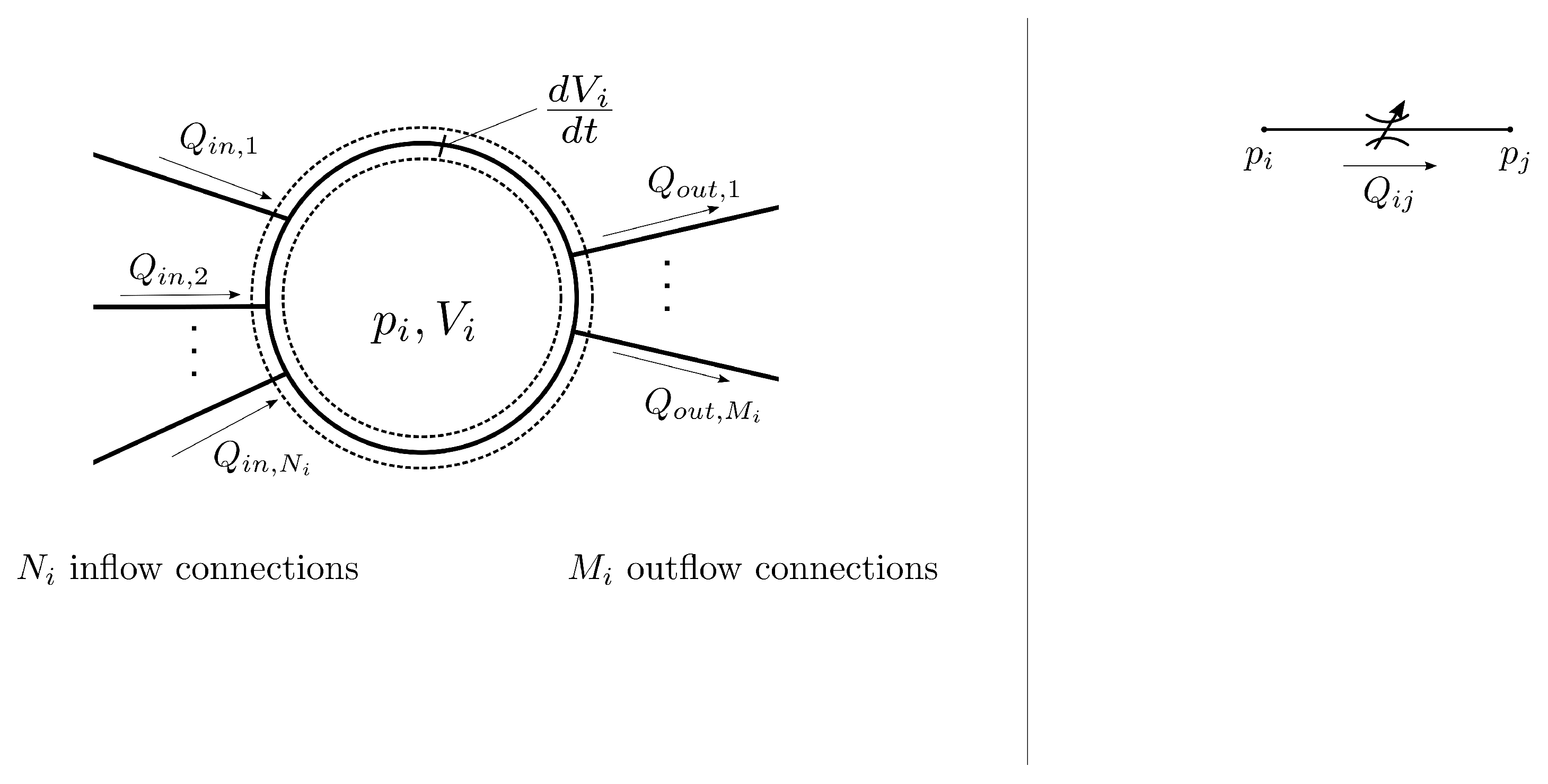
The lumped parameter approach for modeling hydraulic systems is based on the control volume theory, wherein the physical quantities inside each control volume are assumed to be uniform. The entire hydraulic system comprised of the unit is represented in terms of a network of control volumes connected to each other through orifice connections. In each control volume, the pressure is determined using the pressure built up equation [14] which expresses the rate of change of pressure inside a control volume in terms of the flow through connections to the control volume (CV), the volume of the CV, and the bulk modulus of the fluid. The pressure built up equation is given by Equation (1). Figure 1 summarizes the governing equations used in the conventional lumped parameter approach.
In Figure 1, the index i is used to refer to the ith CV in the modeled hydraulic system. In general, the volume of the CV could be varying with time and the contribution from variation in volume is included through the term in Equation (1). The CVs that make up the hydraulic system are connected through hydraulic connections modeled as orifices using the turbulent orifice equation Equation (2) . In practice, the orifice equation (Equation (2)) is an adequate approximation for turbulent flow through hydraulic connections [15,16].
In Equation (2) , represents the volumetric flow rate directed from the ith CV to the jth CV, and are respectively the pressures inside the adjacent CVs i and j, while the area A is the geometrical area connecting the CVs. By convention, sgn denotes the signum function. For dynamic systems such as External Gear Machines (EGMs), both pressures and areas constantly vary with time as described in detail in Section 5. The orifice coefficient is used to include the effect of vena contracta, velocity of approach factor and frictional losses. Dependence on Reynolds number is also incorporated as described in Blackburn et al. [15] and McCloy et al. [17], to extend the use of the orifice Equation (Equation (2)) to the case of transitional or laminar flow. In past work by Shah et al. [13], the conventional orifice equation was modified to account for the compressibility effects through the orifice and is described in detail in Section 3.2.
In situations where the flow is in the laminar regime such as that in flows through gaps moving with respect to each other, a laminar flow approximation obtained from the combination of Couette flow and Poiseuille flow components is used. Such an approximation can be represented in the form of Equation (3). In Equation (3), the flow rate through the gap between CV-1 and CV-2 with pressures and respectively is represented as a superposition of Couette and Poiseuille flow approximations. The equation is applicable for a general gap with h as the gap height, L the gap length, the gap width and v being the relative velocity of a gap wall with respect to a stationary gap wall in observer frame.
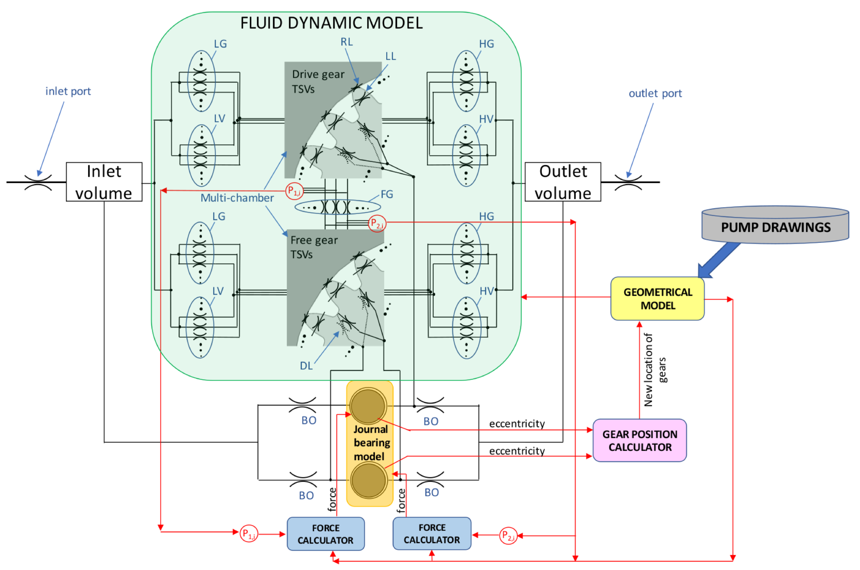
The pressure built up Equation (1), together with the orifice equation and the laminar flow approximations represent a closed system of Ordinary differential equations which can be solved numerically using the External Gear pump simulation tool HYGESim developed by the authors’ team [18]. The overall structure of the HYGESim tool used to solve the system is described in Figure 2. The simulation tool is comprised of a geometric model which reads the geometrical features of the unit through the 3D drawings and computes variation of the various geometric parameters such as the cross-sectional areas of the orifices, the instantaneous volumes of the individual CVs among other parameters. The values of the geometric features computed by the Geometric model are then used by the Fluid Dynamic model to compute the instantaneous flows and pressure inside the system using Equations (1)–(3). The Fluid Dynamic model also computes the instantaneous position of the gears and the effect of the gear position on the flows and interacts with the lateral gap flow solver to determine the gap heights. In this way, the simulation tool can be used to predict the instantaneous dynamical quantities in the system. For additional details regarding the model structure, the reader is referred to Refs. [18,19,20,21,22]. As the major focus of the work is in the development of the cavitation modeling approach, only the Fluid Dynamic model is detailed in the sections that follow.
Further details on the lumped parameter modeling approach for fluid power systems can be found in Refs. [18,19,23]. These past works by the authors’ team have validated the modeling approach with experiments. Dynamic lumped parameter cavitation modeling techniques developed in the past are described in Refs. [11,12,13,24]. The reader can refer to the past works for additional details regarding the modeling approach. This paper follows a similar strategy as that described in [13], but replaces the constitutive equations used to express the rate of growth of phases with physically realizable constitutive relations. Therefore, throughout this manuscript, the main focus will be on the derivation and validation of the appropriate constitutive relations describing the dynamics of bubbles.
3. Cavitation Modeling Approach
A general description of the cavitation modeling approach applicable to dynamic lumped parameter based cavitation models is presented in this section. First a general modeling of fluid properties based on the homogeneous mixture approximation is presented in Section 3.1. Section 3.2 describes how the modeled fluid properties can be incorporated in a lumped parameter approach framework. The resulting equations has production/consumption terms that need to be modeled. A brief description of the approach for estimating these terms for cavitation and aeration is presented in Section 3.3.
3.1. Homogeneous Mixture Modeling of Fluid Properties
As with the cavitation modeling approaches developed in the past works of the author’s team [12,13], the Hybrid Rayleigh–Plesset Equation cavitation modeling approach developed in this paper is desired to be able to account for the effects of compressibility of the fluid inside CVs and through hydraulic connections. Before the proposed model is presented in Section 3.3, the basic cavitation model formulation common to all dynamic lumped parameter cavitation modeling approaches is presented. Proceeding in a manner similar to the previous approaches [12,13], the cavitating fluid is assumed to be modeled as a homogeneous multi-component fluid with the hydraulic oil, gas and vapor components. As a result, all the fluid properties of the mixture can be described in terms of the individual fluid properties and the void fractions of components defined in Equation (4):
where the index i is used to denote either of the three components—oil, gas and vapor present in the mixture. The index j is used to represent the Control Volume in which the void fraction is evaluated. is the Volume of the ith component in the jth CV. The sum of all components within each CV adds up to the total volume of the CV and therefore the void fraction is constrained by Equation (5).
For convenience, the index j is dropped out from the notation hereafter and the fluid properties described refer to those in any arbitrary control volume j. Alternatively, it is convenient to express certain fluid properties in terms of the mass fraction defined in Equation (6):
In Equation (6), represents the mass of the ith component and m the total mass of the fluid. The mass fractions of all components can be defined given the void fractions and vice versa. Therefore, both quantities are used interchangeably in the analysis that follows. With the help of the homogeneous fluid approximation, the density, viscosity and the bulk modulus of the mixture can be expressed in terms of the void fractions of the individual components respectively using Equations (7)–(9). Note that all the fluid properties are considered as a function of pressure only. In general, they would depend on the temperature of the fluid, however, in this study, the system under consideration is maintained approximately at a constant temperature and therefore any variations in fluid properties resulting from a change in temperature are negligible:
In Equation (9), the gaseous components are modeled to undergo polytropic process with polytropic exponent , and consequently the gaseous components bulk moduli are specified using Equation (10). It can be noted from Equation (9) that the presence of a small amount of gas phase components can cause a sharp decline in the overall bulk modulus of the system and therefore the presence of cavitation or aeration bubbles can significantly alter the dynamics of the hydraulic system being modeled:
3.2. Dynamics of Homogeneous Mixtures in Control Volumes
In the presence of the gas phase components, the compressibility of the mixture is lower than the compressibility of the oil. For consistency, such changes in compressibility need to be accounted for in the governing equations Equations (1) and (2) for the lumped parameter approach described in Section 2. Inclusion of the compressibility effects in the pressure built up equation (Equation (1)) is relatively straightforward and can be achieved using the effective bulk modulus of the fluid Equation (9) as the bulk modulus in Equation (1), whereas compressibility effects in flow through connections can be embedded in the Energy equation to arrive at the compressible orifice equation [24]. It is convenient to express the flow through the orifice in terms of the mass fractions using Equation (11) [24].
As before, i and j represent indices corresponding to the ith and the jth CVs, respectively, A is the area of the cross section normal to the flow direction, and the bulk modulus of the liquid phase at a reference pressure . The terms and represent the vapor and gas mass fraction in the mixture evaluated at the chamber upstream of the flow direction. The additional term W comprises of the boundary work done on or by the gas phase components in compression or expansion expressed by Equation (12). A detailed explanation of how this term is derived is given in Appendix A The effects of viscous dissipation are assumed to be factored in the coefficient of discharge :
The analysis presented thus far expresses the dynamical quantities such as the pressure in a CV and flow rate across connections in terms of specified fluid properties of individual components and the gas and vapor mass fractions. The gas and vapor mass fractions themselves vary continuously with time, pressure and flow through the system. Therefore, to close the system of equations, expressions relating the mass fractions with the dynamical quantities need to be derived considering the transport of phases across the components, which can be described using a transport equation [13] using Equation (13):
wherein and for the kth chamber are given by:
The last term on the right side of Equation (13) represents the rate of change of the gas or vapor mass fractions due to phase change. This term, referred to as the source term, requires additional modeling and must reflect the dynamics that occur during phase change processes resulting in the generation or destruction of phase mass fractions. Modeling approaches for this term are addressed in the following section.
3.3. Closure Relations for Cavitation and Aeration
In order to establish a closure to the system of equations, the source term in Equation (13) needs to be specified. The specification of the source term depends in general on the thermodynamic processes that occur during phase change. For solving the dynamics of a lumped parameter system such as the EGM case, the thermodynamic processes that occur during phase change and the change in corresponding physical quantities cannot be assessed at each instant of time. Therefore, the source term requires additional modeling.
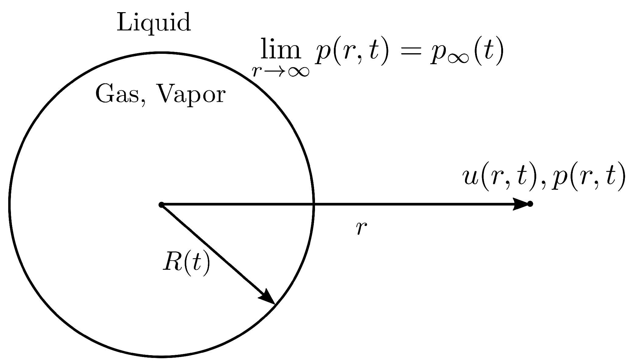
It is desired that with the modeled source term come equations representative of the underlying physics of phase change and bubble dynamics. The well known Rayleigh–Plesset equation [25,26] can be used to describe the dynamical evolution of a spherical bubble placed in infinite fluid medium [27,28]. For a bubble schematic shown in Figure 3 with pressure away from the interface and inside the bubble assumed uniform, the Rayleigh–Plesset (RP) equation reads as:
In Equation (16), represents the coefficient of surface tension between the liquid and gas/vapor components and denotes the kinematic viscosity of the liquid component. The first two terms on the left-hand side of the equation are due to the unsteady evolution (acceleration) and advective transport. On the right-hand side, the first term is representative of the forces exerted due to the pressure difference in the fluid, the second term is representative of the viscous forces at the bubble interface while the last term indicates the forces due to surface tension.
Previous cavitation modeling efforts have used the RP equation [7,12,13] to develop suitable models for the source term. The RP equation in itself is a nonlinear equation for which explicit analytical solutions cannot be obtained. Therefore, approximations are made to derive a model for the source term from the RP equation. The approximations used in Refs. [7,12,13] referred to as the asymptotic limit approximation, neglect the viscous dissipation, the surface tension and the acceleration terms and conveniently express the instantaneous evolution of the radius of the bubble in terms of the pressure term in the RHS of Equation (16) as given in Equation (17). Although the final form of the modeled term is different in different modeling strategies, Equation (17) is the basis of all the dynamic cavitation models derived in Refs. [7,11,12,13,22]:
The asymptotic limit approximation lacks the nonlinear contributions of the unsteady evolution term and it will be shown later that it may result in inaccurate prediction of the time-scales of bubble growth or dissolution under certain conditions. As a result, these dynamic cavitation models are not physically realizable. The proposed modeling approach is aimed at overcoming this drawback by retaining the nonlinear contributions in the RP equation.
In addition to the RP equation, the Henry’s law is used to determine the pressure due to gas content inside the bubble. According to the Henry’s law, the partial pressure of the gas in the bubble which is in equilibrium with a saturated concentration of the gas is given by:
In Equation (18), H stands for the Henry’s constant which is the constant of proportionality in Equation (18). Analogous to the expression for the growth of vapor mass fraction at pressures below the vapor saturation pressure, expressions consistent with equilibrium mass fraction in Henry’s law could be obtained and solved in combination with the RP equation to model the source terms for both gas and vapor components.
4. Hybrid Rayleigh–Plesset Equation (RPE) Model
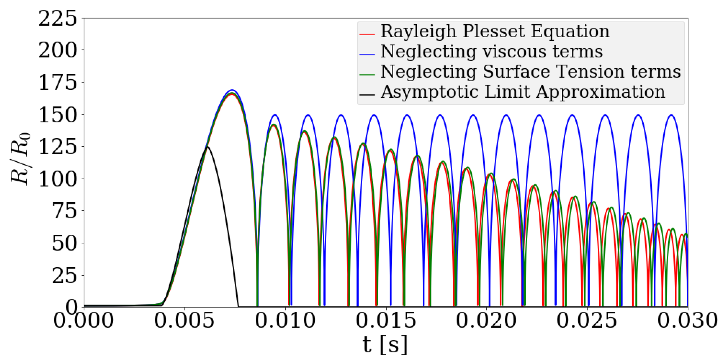
As described in the previous section, the existing dynamic models with asymptotic limit approximation leads to unrealistic prediction of the timescales of bubble growth or dissolution. Now, the contribution of different terms in the RP equation in predicting the time scales of bubble growth are illustrated. Starting with a bubble of radius , the pressure away from the bubble is forced in a manner shown in Figure 4. As the pressure far away from the bubble is reduced below saturation pressure, the bubble tends to grow and collapses on recovery of the pressure. This can be realized as a situation typical of a cavitating nucleus which grows upon experiencing pressures lower than saturation pressure and implodes as the pressure increases beyond saturation pressure. Due to inertial effects, the bubble is expected to undergo series of collapse and rebound cycles before it ceases to exist. The RP equation can be solved numerically to obtain the evolution of the bubble radius and these trends in bubble growth and collapse can be verified from the solution shown in Figure 5. The time scale of the bubble can be determined from the time required by the bubble to approach its initial size in the fluid. Also shown in Figure 5 are the solutions to the RP equation, neglecting separately the contribution from the viscous term, surface tension term and the asymptotic limit approximation as in Equation (17). It can be observed from Figure 5 that neglecting the viscous term in Equation (16) causes the bubble growth-rebound cycle to go on indefinitely, implying that the viscous terms have a significant contribution in the determination of the timescales of the growth-rebound cycles. On neglecting the surface tension terms, one can observe from Figure 5 that the surface tension does not play a crucial role in determining the time scales of bubble growth or dissolution. If both the surface tension and viscous dissipation terms are neglected and the unsteady evolution term is neglected, the asymptotic limit approximation is obtained. From Figure 5, it can be observed that the asymptotic limit approximation grossly under-predicts the timescales of bubble growth and collapse, which necessitates the formulation of a model capable of predicting the bubble evolution and the source term accurately. This section details the proposed approach to model the evolution of bubble growth.
4.1. Basic Model
In order to describe the proposed model, certain simplifying approximations need to be introduced first. In the proposed approach, the homogeneous mixture is considered to comprise a homogeneous bubble distribution with a specified bubble number density N assumed uniform in a CV. With this assumption, the rate of change of the void fraction of vapor and gas components can be expressed in terms of the rate of volumetric expansion of the bubbles as:
Equation (19) shows that the model can evaluate the evolution of the void fraction of the gas or vapor components once the evolution of bubble radius is known. The source term for the transport equation in Equation (13) can be modeled given the relationship between the void fraction and the mass fraction in Equation (6). Therefore, the problem of specifying the source term is now reduced to determining the radius of bubbles confined for their corresponding CVs. The proposed approach devises a numerically efficient procedure of determining the radius of the bubbles for their respective CVs and is elucidated in the sections that follow.
4.2. Averaged Rayleigh–Plesset Equation
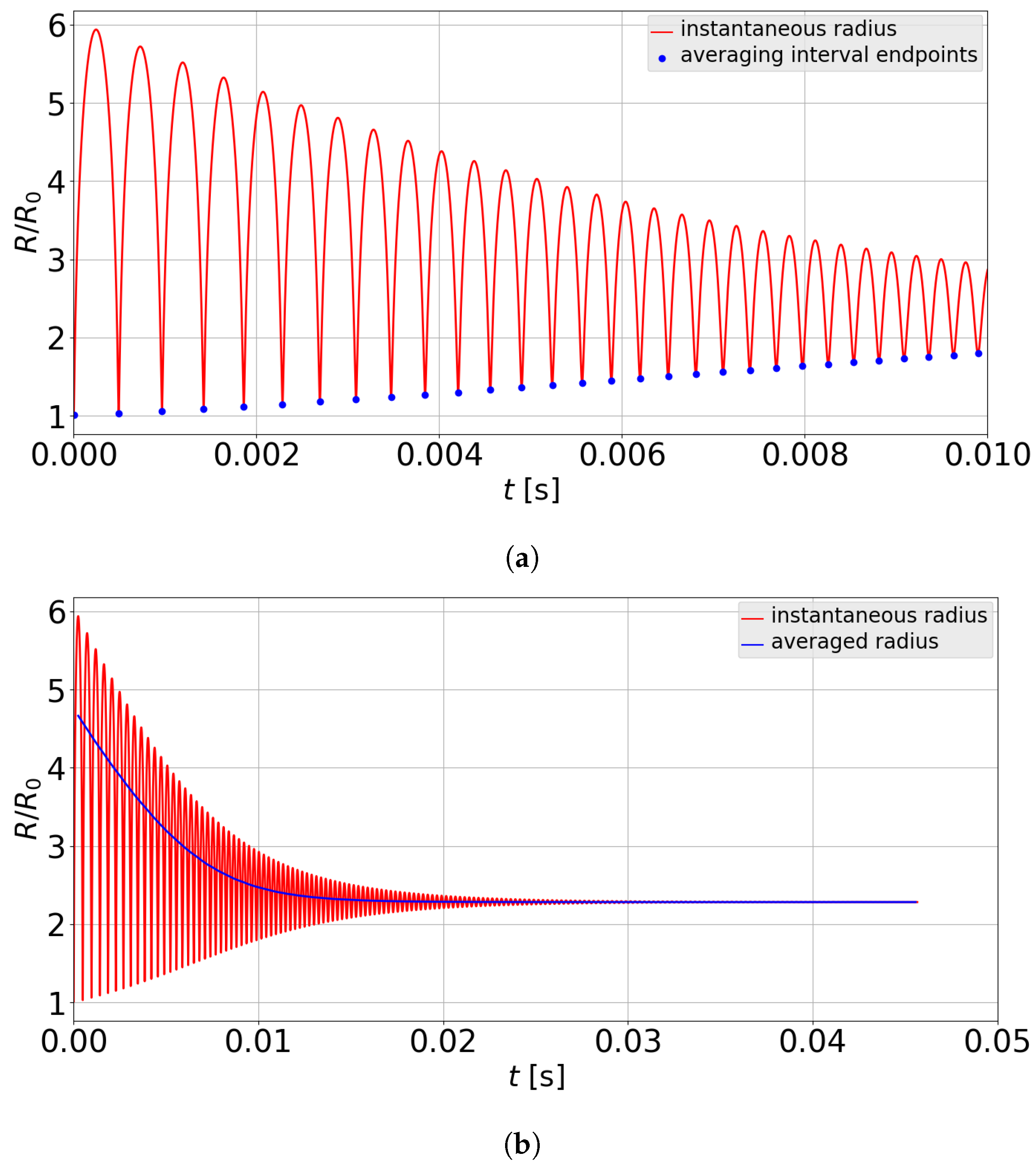
The proposed model for the source term couples the RP equation with the other governing equations (pressure built-up equation, compressible orifice equation, transport equation) in the determination of the dynamics of the hydraulic system under study. RPE equation (Equation (16)) is known to exhibit stiff behavior owing to the nonlinear acceleration term making it difficult to obtain converged numerical solutions to the problem. The coupling of the RP equation with the other equations further aggravates the convergence of numerical solution. For a complex hydraulic system consisting of multiple CVs and hydraulic connections such as an EGM, a converged numerical solution may not be obtainable in reasonable computational time. Furthermore, the instantaneous radius of the bubble in a growth-collapse process as shown in Figure 5 is not crucial to the prediction of the overall trends of dynamical quantities of the hydraulic system such as the pressure in a CV or the flow rates across hydraulic connections. It must be emphasized here that, although the instantaneous radius is not imperative to the prediction of dynamical features of the system, a measure of the timescales of the bubble growth or dissolution process is necessary for an accurate prediction of the system dynamics. Therefore, the proposed modeling approach attempts to solve the averaged Rayleigh–Plesset Equation. The solution to the RP equation is averaged to obtain the overall trends in the void fraction as well as the damping time of the bubble growth-rebound cycles. Figure 6 presents a comparison between the averaged and instantaneous solution to the RP equation. The averaging interval chosen in this case is shown by the solid marker points in Figure 6a. For the averaged solution to be consistent with the underlying dynamics, it is desired that this averaging interval be small enough to predict overall trends. For the case of a bubble set in growth rebound cycles during cavitation, the averaging interval defined by consecutive rebound time instants was determined to be sufficient to capture relevant dynamics. The proposed approach is aimed at predicting the solution to the RP equation in the averaged sense and subsequently determine the source term.
4.3. Energy Equation for the Bubble Placed in an Infinite Fluid Medium
From the analysis presented thus far, it is clear that a closure cannot be established directly from the momentum equation (RP equation) alone. It is instructive to study the energy equation for a bubble placed in infinite fluid medium. The analysis of the energy equation reveals that the nonlinearity in the momentum equation is embedded in the behavior of the evolution of the kinetic energy of the fluid surrounding the bubble. The energy equation for a single bubble placed in an infinite fluid medium can be expressed in terms of the kinetic energy k of the fluid as:
It is useful to identify the contributions from different terms in the energy equation to facilitate model reduction. In Equation (20), the first term on the Left Hand Side (LHS) denotes the unsteady evolution of the kinetic energy. The unsteady evolution term in Energy equation combines both the nonlinear terms in the momentum equation and is linear in the Energy equation. The linearity of the unsteady term in the Energy equation therefore makes it easier to model the nonlinear contributions from the momentum equation. This justifies the use of an additional Energy equation to arrive at the model. The second term on the LHS denotes the transport of the kinetic energy into or out of the domain. The first term on the Right Hand Side (RHS) represents the boundary work done by the gas inside the bubble and the work done by the normal stresses at the domain boundary. Depending on the sign of and the pressure difference , this term could be either positive or negative. The second term on the RHS of Equation (20) denotes the viscous dissipation of Energy. Consistent with the second law of thermodynamics, this term always remains negative due to the appearance of . The last term on the RHS denotes the contribution from the surface tension forces. This term can be positive or negative depending on whether the interface area is increasing or decreasing. It is important to emphasize that the contributions of Energy from the pressure and surface tension forces are recovered as the system is brought back to its initial state, however, that due to viscous dissipation is lost into heat and cannot be recovered spontaneously. During the bubble collapse and rebound process, the energy due to expansion work and the surface energy will vary cyclically and cause the kinetic energy to fluctuate making it difficult to model. This difficulty can be circumvented if the total energy is modeled instead. The total energy is defined as:
Here, T denotes the transported kinetic energy and G denotes the contributions of energy from the pressure and surface tension forces. By integrating the volumetric dissipation rate around the bubble, an expression for the viscous dissipation rate can be obtained in terms of the kinetic energy as:
The energy equation can be rewritten using the definition of the total energy and the dissipation rate as:
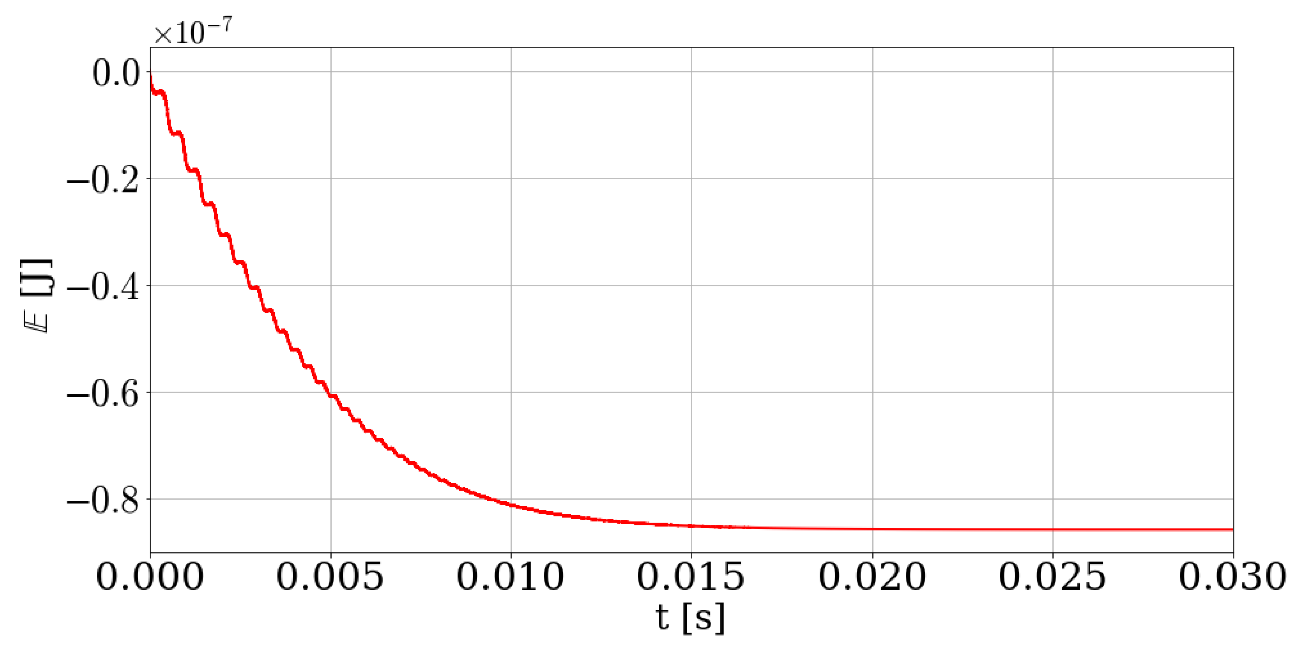
Due to the appearance of the non-negative viscous dissipation term in Equation (23), the total energy is expected to decrease monotonically from its initial value until it reaches a constant value. This is demonstrated with an example shown in Figure 7. In this example, the bubble is forced into expansion by introducing a step change in pressure far away from the bubble interface given by:
4.4. Dimensional Analysis of the RP Equation
The RP equation is non-dimensionalized to understand the relationship governing the energy dissipation rate with the input parameters. The idea is to solve the RP equation with a step change in pressure input for different values of input parameters— and express a relationship of the dissipation rate and energy. Three repeating (independent) parameters are required corresponding to the dimensions of Mass, Length and Time to fully specify the non-dimensional relationship. In what follows, the steady state energy , density and the steady state radius are chosen as the independent parameters, as they are uniquely defined for a given initial state. With this choice, the dependence of the total energy could be expressed as:
where f is a function expressing the non-dimensional relationship.
Using the Buckingham theorem, the following non-dimensional groups are identified:
The non-dimensional group are used to understand the effect of initial radius of the bubble, variation in the prescribed step pressure function, and the surface tension effects. The dimensionless viscosity represents the effect of the fluid viscosity. The parameters and are the dependent parameters that need to be expressed in terms of the aforementioned groups. The non-dimensionalized time can be formed in a similar manner using the independent parameters and as:
The steady state radius of the bubble can be determined implicitly for the step pressure input, by substituting in the RP equation. This leads to:
where is the initial pressure of the gas component inside the bubble. For a bubble initially at equilibrium, is related as . With this relationship, Equation (33) can be rewritten in terms of the group after multiplying both sides by as:
Equation (34) specifies a relationship between the non-dimensional groups , and . Therefore, one of the groups is not independent and can be eliminated. Without loss of generality, the group is chosen to be eliminated from the analysis, leaving behind three independent groups— and . The reduced relationship between to be explored groups can thus be written as:
Alternatively, the time dependence of energy can be removed knowing that the rate of change of energy depends on the dissipation rate (Equation (23)) and the dimensionless dissipation rate can be expressed as:
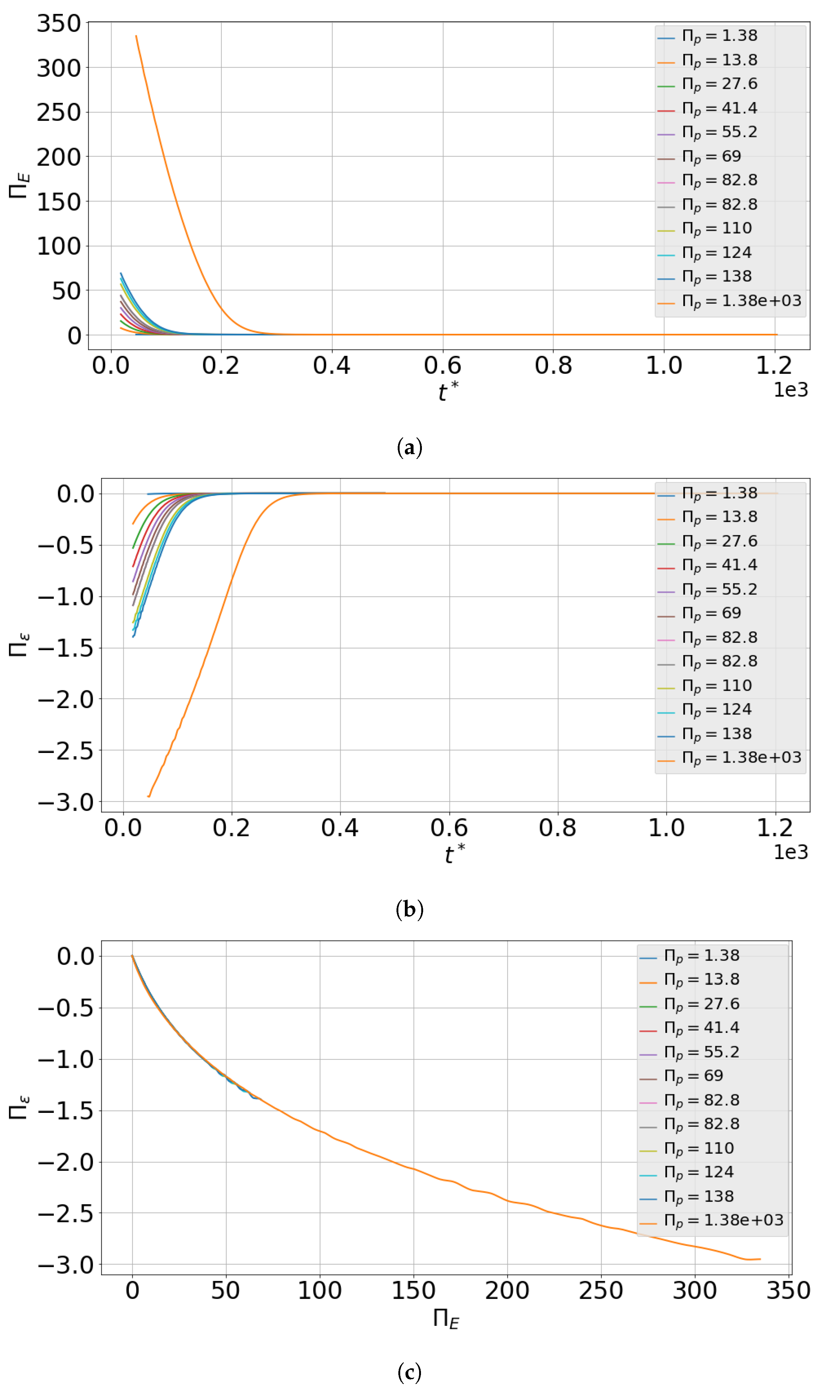
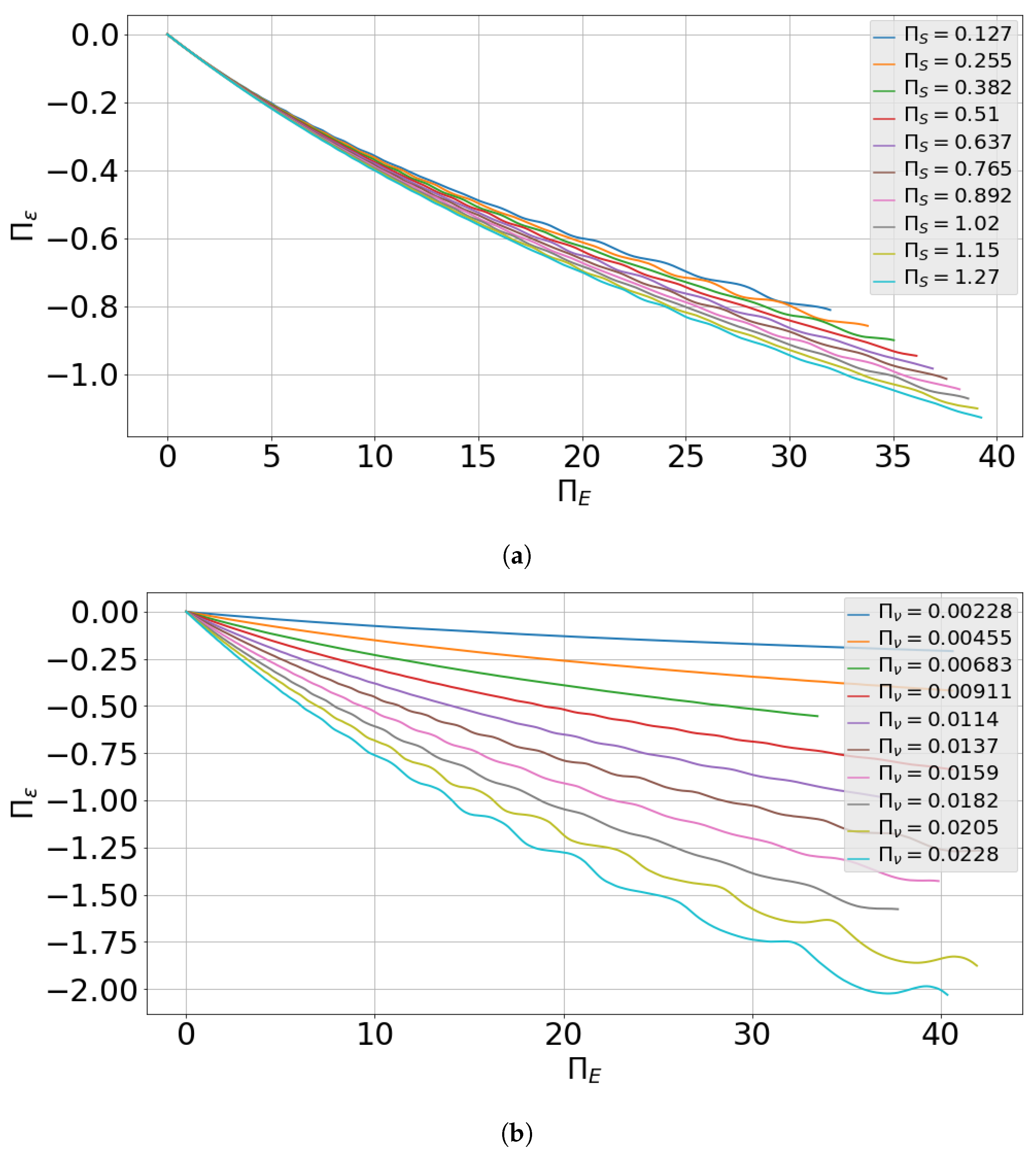
Now, the non-dimensional relationship between the dimensionless dissipation rate and dimensionless energy for varying values of is explored. To that end, simulations were performed by varying groups independently. A baseline case with , and is constructed considering a bubble with an arbitrary initial radius of 1 mm initially placed in hydraulic fluid at a temperature of 50 °C and absolute pressure of 1 bar. The magnitudes of the groups are varied so as to observe the dimensionless relationship for the range of possible variations in physical quantities in the operation of a typical EGM. Figure 8 shows the variation of the dimensionless energy and dimensionless dissipation rate with dimensionless time as well as with each other. It can be observed from Figure 8a,b that the dimensionless energy as well as the dissipation rate reach steady state at different dimensionless times for different values of . However, when they are viewed together on a single plot as in Figure 8c, the variation between and appears to be independent of the value of . Thus, the dimensionless relationship between the dissipation rate and the Energy can be further reduced with the only independent parameters being and . Likewise, simulations performed with different values of and respectively indicate weak dependence on (Figure 9a) and strong dependence on (Figure 9b). A power law relationship is observed to describe well the trends between and . Therefore, the reduced relationship between dimensionless dissipation rate and dimensionless energy can be cast into the following form:
Here, a is a function of the dimensionless viscosity . It was discovered that this function varies linearly with and is 0 for making it consistent with the solution to the original RP equation.
Thus, the final relationship between and may be expressed as:
with the constants , and determined numerically so as to minimize the overall error between the original solution and the modeled equation.
In an analogous manner, the relationship between the dimensionless volume and dimensionless energy can be determined. For brevity, only the final relationship is presented without going into the details of dimensional analysis for dimensionless volume. The following form of the Volume equation is identified to predict the solution accurately:
In Equation (39), a is a cubic polynomial in given by: and . The mimimum error across all cases was determined to be about . The proposed model is now complete with the addition of the non-dimensional relationship for the volume of the bubble. At any given instant of time, if the energy of the system is known, the averaged dissipation rate can be computed and the energy for the next time instant can be determined in an averaged sense using Equation (23). Thus, the energy can be determined at all instants in time. With Equation (39), the radius of the bubble also can be determined and hence the void fraction and the source term can be computed, thus completing the set of governing equations.
To summarize, the full set of equations solved in the cavitation model within each CV and the hydraulic connections across them can be summarized as follows:
In Equation (40), the last two equations governing the evolution of the dimensionless quantities replace the evolution equation of the bubble radius and the kinetic energy when the system becomes stiff.
4.5. Validation Tests and the Hybrid Modeling Approach
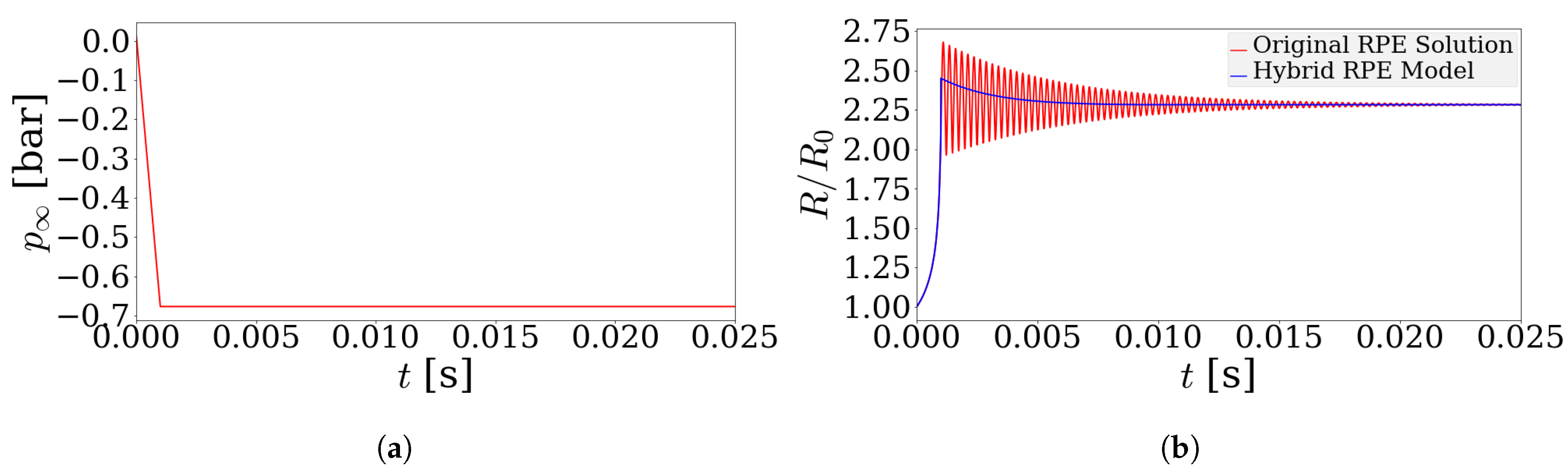
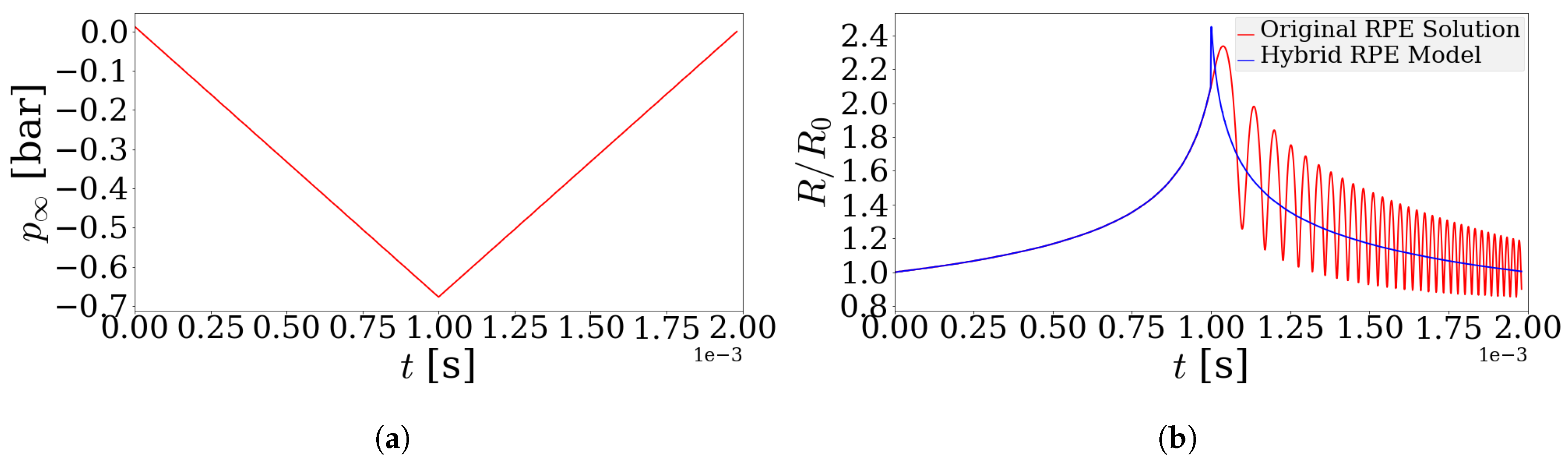
The proposed approach has been developed for a step pressure change away from the bubble interface, however, it is desired that the model work for all possible pressure variations that occur in a generic hydraulic system. A hybrid model is proposed, wherein the original RP equation is solved in the intervals of time where the system behavior is not stiff and the power law approximation is used in the regions where the system behavior is stiff and exhibits strong gradients such as in the growth and collapse cycles experienced by the bubble during cavitation or aeration. The hybrid model overcomes these difficulties and models the solution accurately such as in the case with linear variation in pressure as shown in Figure 10. The hybrid model solves the original RP equation between and the during which the pressure declines linearly. During this phase, the system does not exhibit stiff behavior and the original RP Equation is solved numerically. As soon as the pressure reaches the saturation pressure at , the bubble is set into series of growth and rebound cycles and the system becomes numerically stiff to solve. During this time, the solver switches over to the power-law approximation developed in the preceding section. As can be seen in Figure 10b, the power law approximation agrees with the solution to the RP equation in the averaged sense and predicts the time scale of bubble growth and the steady state radius quite accurately. The hybrid approach has been validated for several different pressure variations forced upon the bubble, and for brevity, only one example validating the hybrid model is illustrated in Figure 11. The Hybrid RPE model matches the solution to the RP equation and is computationally inexpensive to solve as the stiff regions of the RP equation are replaced by explicit power-law approximations to the RP equation. This model can be easily implemented in a lumped parameter model to incorporate and solve for cavitation as well as aeration for a complex hydraulic system. The following section details the implementation of the proposed hybrid modeling approach.
5. Implementation of the Proposed Model in HYGESim Tool
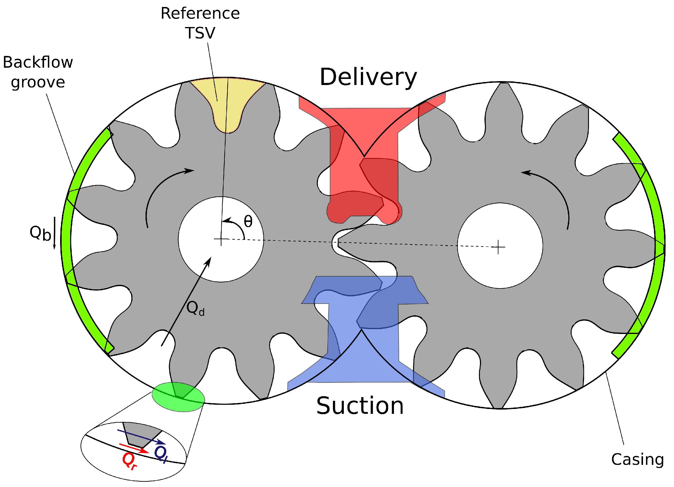
In modeling EGM using the lumped parameter approach, the fluid domain between the gears and the casing is divided into partitions equal to the sum of teeth on the drive and driven gears. Each of these partitions (TSV) is considered as a separate CV connected with other CVs using suitable hydraulic connections. To represent the inlet and outlet environments, additional stationary CVs are defined and are connected to the TSVs through the suction and delivery ports. A simplified representation of an EGM unit is shown in Figure 12. Shown in the figure are the different TSVs, of which the reference TSV is highlighted. Several different connections across the TSVs represent the leakages that occur through radial and lateral gaps and connections across the backflow groove highlighted in green in Figure 12 are considered. In addition, drain leakages and flow through grooves are also modeled. Additional details on the leakage connections can be found in [18].
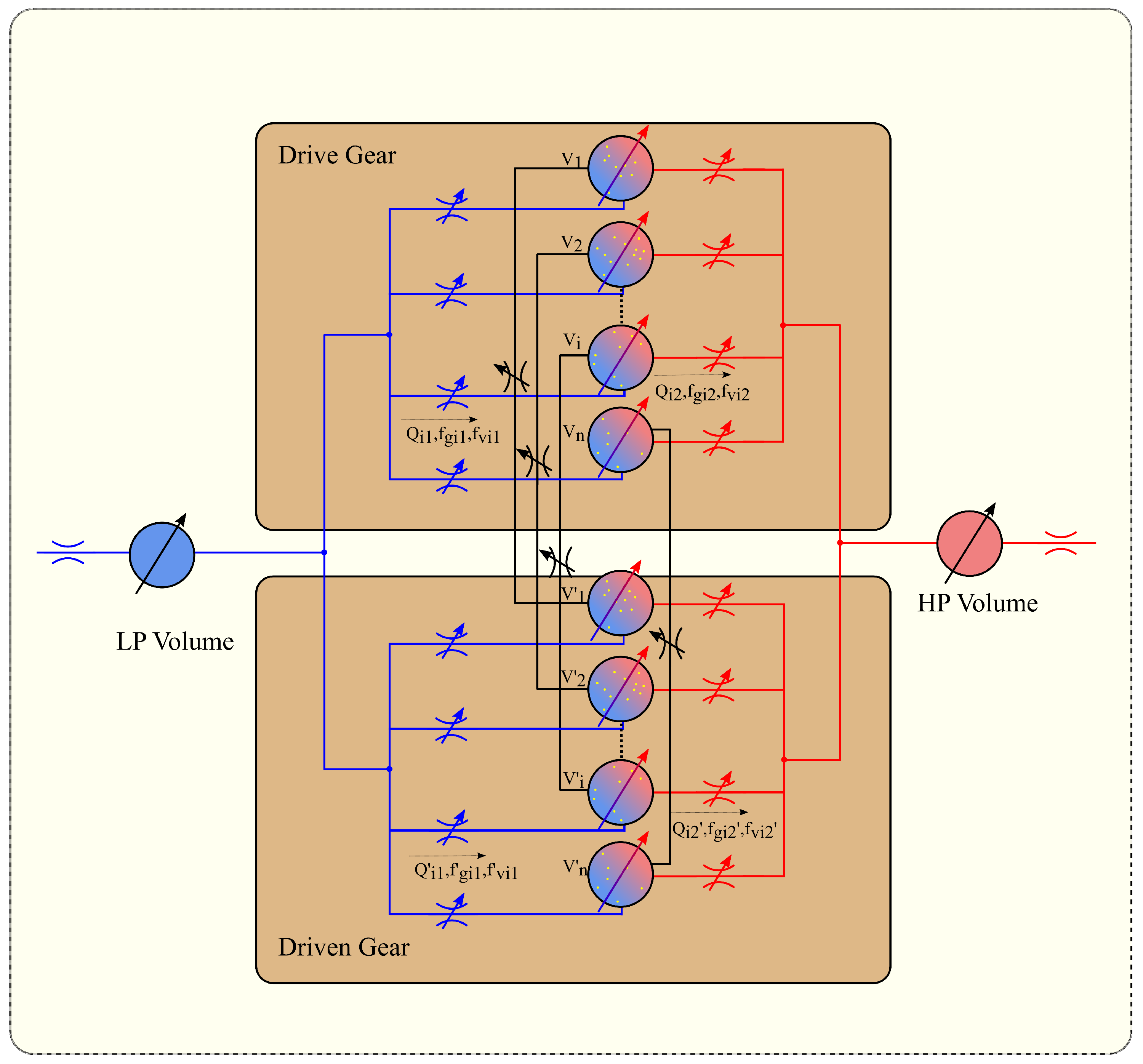
A representation of the EGM model in terms of different CVs and hydraulic connections is shown in Figure 13. The entire system is represented in the form of a network of CVs and hydraulic connections. Each of these CV has in general a volume that varies with the rotation of gears. The opening through the different connections are computed by the geometry model from the Computer Aided Design (CAD) data.
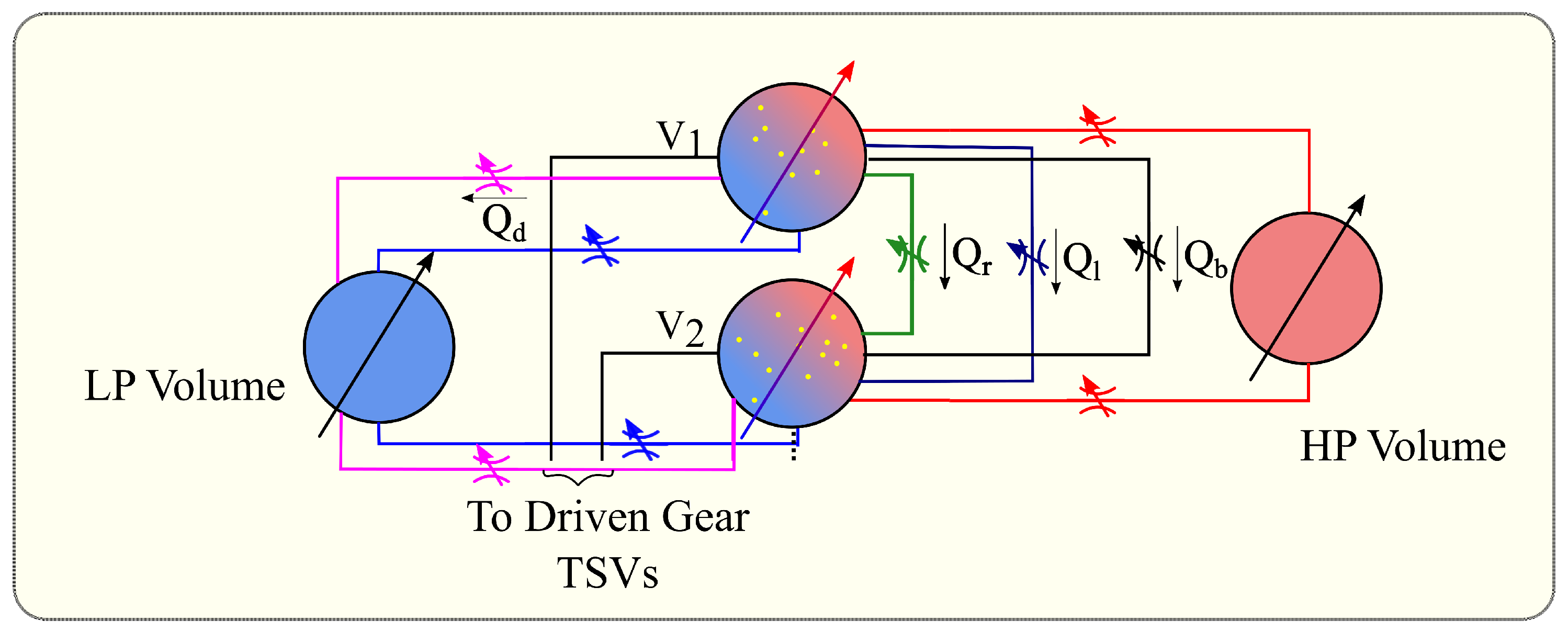
The entire unit can be assumed to be made up of CVs with representing the Volume of the ith TSV in the drive gear and that of the driven gear. Each TSV is connected to CVs at suction and delivery side (denoted respectively by Low Pressure (LP) volume and High Pressure (HP) volume in Figure 13 by orifices with variable opening). For illustration, the leakages across adjoining TSVs, drain and the flow through the backflow groove are not shown in this figure, but instead shown magnified in Figure 14. It shows the radial leakage connections (), the lateral leakages (), drain leakages () and the backflow groove connection () between TSVs 1 and 2. Although shown only for TSVs 1 and 2 in Figure 14, these connections are modeled for all the TSVs corresponding to the drive and the driven gear CVs. For illustration, all the connections described here are shown as variable orifices in Figure 13 and Figure 14; however, not all connections are modeled as orifices. The leakage connections , and are modeled using the laminar flow approximations determined by Equation (3) with the corresponding gap height and wall velocity. Some of the characteristic specifications of the unit are listed in Table 1.
All the HYGESim modules shown in Figure 2 are implemented in C++ and in particular the Fluid dynamic model is implemented as a system of Ordinary Differential Equations (ODE) solved by the LSODA solver [29]. The LSODA solver solves for the system of ODE which can be represented as:
All simulations performed in this study were converged within a maximum residual error of 0.01% in the LSODA solver.
6. Experimental Setup
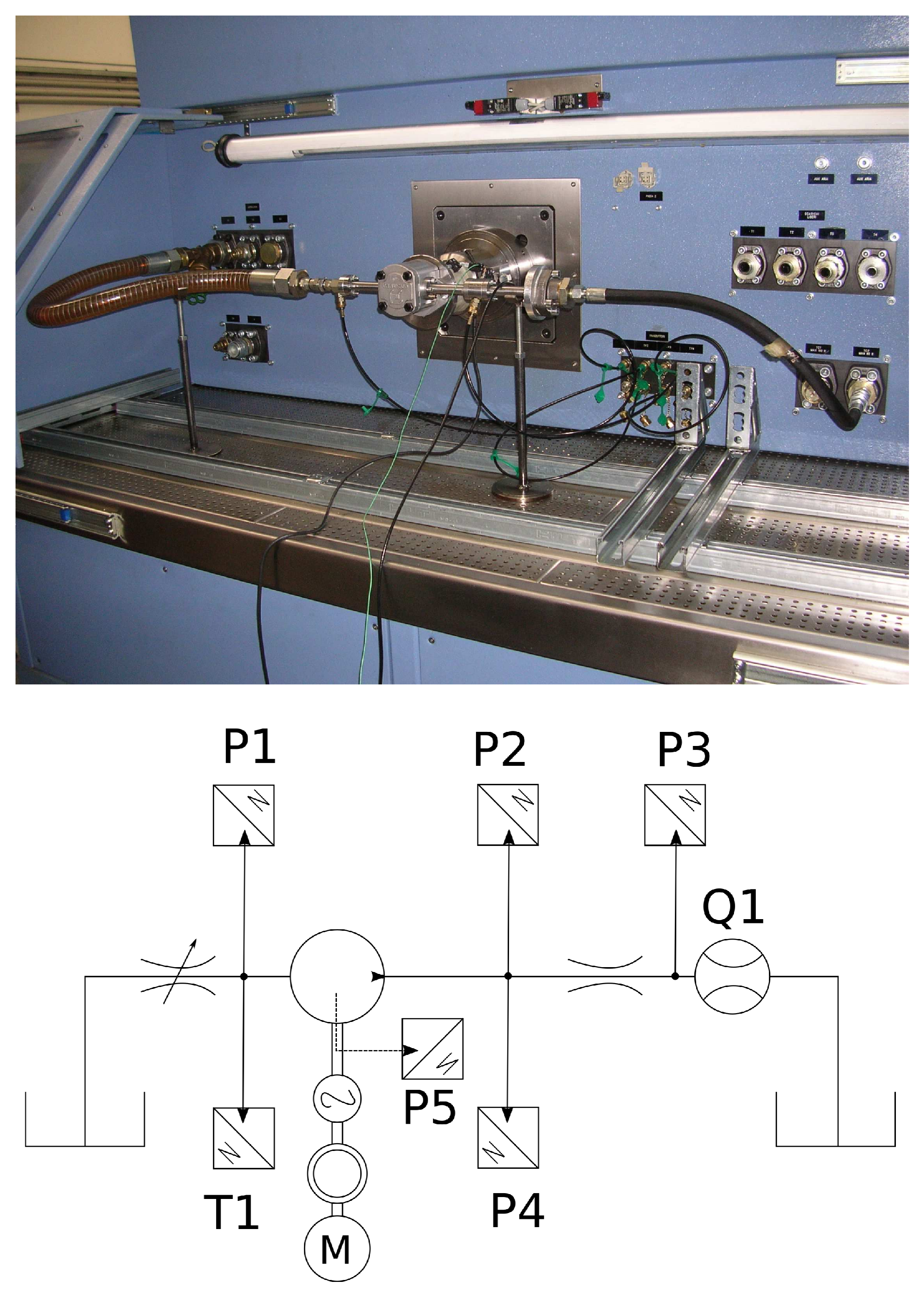
The experimental setup used for validation of the proposed model is the same setup described in previous works [12,13] for model calibration. For completeness, a short description of the set up is described herein. An experiment was performed at the Fluid Power Laboratory of the University of Parma, Italy to measure the flow parameters of the reference commercial EGM. A variable orifice was used as a load for the pump and adjusted to achieve the desired delivery pressure. At the inlet, a variable orifice was used to constrict flow and induce cavitation at the inlet. The experimental setup and its ISO schematic are shown in Figure 15, respectively. A variable frequency drive connected to an electric motor is used to measure and specify the desired shaft speed. For the measurement of the instantaneous pressure inside the TSVs, a piezoresistive micro-transducer with a receptive head diameter was drilled inside the root surface of the drive gear. Additional details on the sensor placement are reported in Refs. [12,30,31]. Instantaneous pressure at the inlet and the outlet of the pump was measured with the help of pressure sensors P1–P4 as shown in the schematic of Figure 15. The flow meter Q1 was used to measure the averaged flow rate at the delivery side. Additional details pertaining to the sensor accuracy are listed in Table 2.
Several experimental tests were performed to observe the cavitation characteristics of the unit. The operating fluid used was hydraulic oil VG46. During the tests, the temperature of the oil was maintained at about 50 °C. The unit was tested at different operating speeds and delivery pressures.
7. Simulation Results and Validation
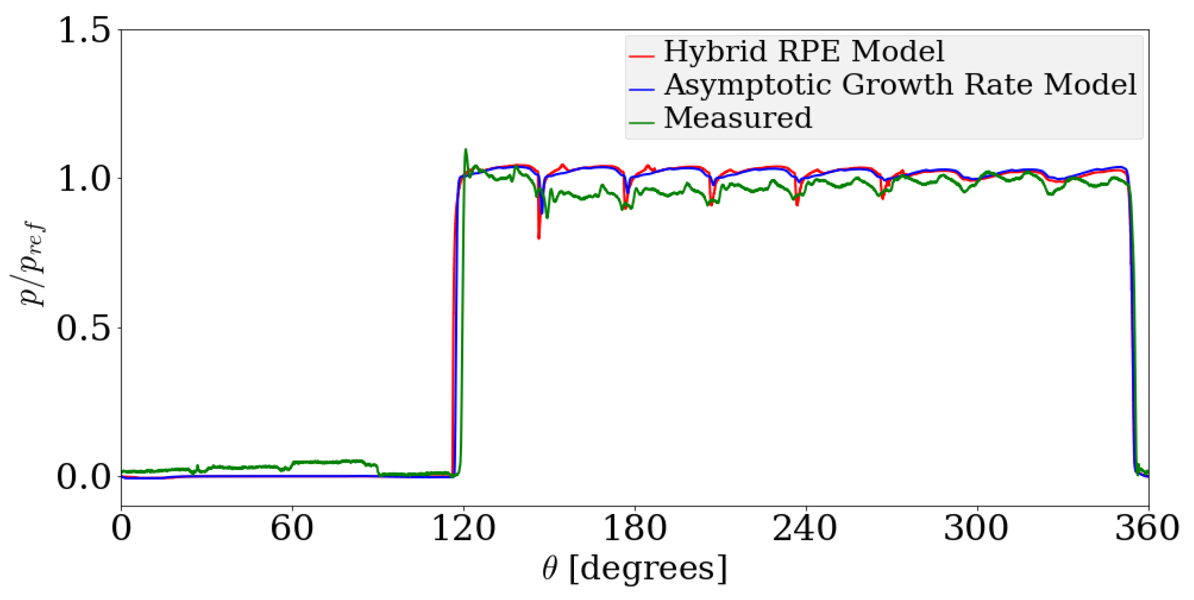
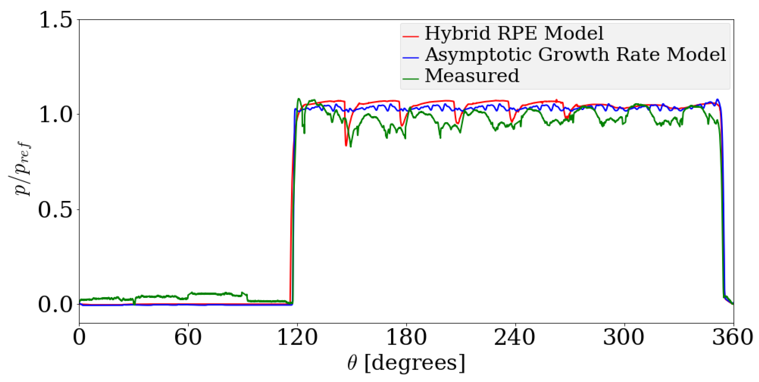
Simulations were carried out to validate the proposed Hybrid RPE modeling approach with experimental data for the reference case unit. While the void fraction of gas and vapor components can be analyzed using Equation (19), the focus in this study is to estimate the performance of the unit and therefore only the pressure and flow rate variables are studied. More specifically, here the overall flow rate through the unit and the pressure inside a reference TSV and delivery port are analyzed. The Hybrid RPE approach requires specification of the initial radius of the bubbles in the chamber, the bubble number density and the threshold dissipation rate to determine the solution at any given instant. For this particular case, the parameters were chosen heuristically to be m, bubbles/m and J/s per bubble. In addition, comparisons are made with the existing dynamic cavitation modeling approach introduced in ref. [13]. For the purpose of discussion, this model is here referred to as the Asymptotic Growth Rate model as it uses the asymptotic bubble growth rate limit in the formulation of constitutive equations. The relaxation parameters required by the Asymptotic Growth Rate model were chosen to be , , and and a saturated air content of 8% by volume. This choice of parameters was obtained using an iterative optimization procedure so as to minimize the RMS error between the simulated and experimentally observed pressure profile. Comparisons were also made with the static model of AMESim (Version 14, Siemens Munich, Germany) and the results were found to consistently produce a larger error compared with the dynamic cavitation models. Such observations are well known and have also been reported previously with other units in Refs. [12,13,24]. Therefore, only the results from dynamic models are discussed in the remainder of this section. Simulations carried out using the dynamic models show good agreement with the experimental results for all operating conditions. For illustration, comparisons for three reference cases are shown among other cases to include the operating conditions ranging from mild to extreme cavitating conditions. Figure 16, Figure 17 and Figure 18 show a comparison between the two dynamic cavitation models—the Hybrid RPE model and the Asymptotic Growth Rate model for the operating speeds of 1000 rpm, 1500 rpm and 2000 rpm. The simulated mean flow rate through the unit are tabulated in Table 3 in terms of the reference flow rate chosen to be the experimentally measured flow rate for their respective operating speeds.
Before analyzing the performance of the proposed cavitation, it is important to observe the general trends in measured quantities in the unit under cavitation conditions. Figure 16, Figure 17 and Figure 18 show the pressure inside a reference TSV plotted against the angular position of the TSV measured from the reference position shown in Figure 12. For comparison, the pressure is non-dimensionalized by a reference pressure held constant during the simulation. One can observe that there are eight large-scale variations in the high pressure regions of the instantaneous pressure profile. The number of high-pressure ripples is related to the number of TSVs in which the fluid pressure is high at any given instant of time. There are in total 12 teeth in the unit (see for example the schematic from Figure 12); however, the eight large-scale ripples are characterized by the number of TSVs between the start of the backflow groove highlighted in green in Figure 12 and the delivery side as the TSV goes from suction to delivery side. The backflow groove establishes a connection between the TSVs where the fluid is not pressurized to the TSVs where the fluid is at a higher pressure enabling pressurization of the fluid at an earlier angular rotation. In this case, there are eight teeth between the low pressure end of the backflow groove and the delivery side resulting in eight large-scale pressure ripples.
As the pressurization of the TSV begins, the pressure inside a TSV spikes initially at about 120° from the reference and plummets significantly after it has rotated by about 24°. This decline in pressure is observed cyclically with each progressive decline being lesser than the preceding one. This trend becomes stronger as the operating speed and the extent of cavitation increases. This suggests that the observed trend is due to cavitation in the unit. As the pressure inside the TSV drops below the saturation pressure (assumed to be bar and bar gauge pressure), the gas and vapor mass fractions tend to increase gradually and persist even as the pressure inside the TSV increases beyond the saturation pressure. The reference TSV experiences a low pressure between 0°–12° of rotation, where the gas and the vapor void fraction increase and, as the TSV reaches the regions of high pressure, the condensation or dissolution process has not completed. The presence of gas or vapor components during the pressurization phase causes a drastic decline in the stiffness of the system and consequently the pressure inside the TSV plummets as the TSV loses flow through gaps and the backflow groove. This trend decreases as the gas and vapor mass fractions decrease in subsequent cycles.
For the case of 1000 rpm operating speed shown in Figure 16, mild cavitation is observed as the pressure at the inlet is just below the gas saturation pressure assumed to be bar gauge pressure. The initial decline in pressure in Figure 16 is overpredicted by the Hybrid RPE model, whereas the Asymptotic Growth Rate model predicts a lower decline in pressure. Following the initial decline in pressure, the Hybrid RPE model predicts the pressure more accurately compared with the Asymptotic growth rate model in the subsequent cycles.
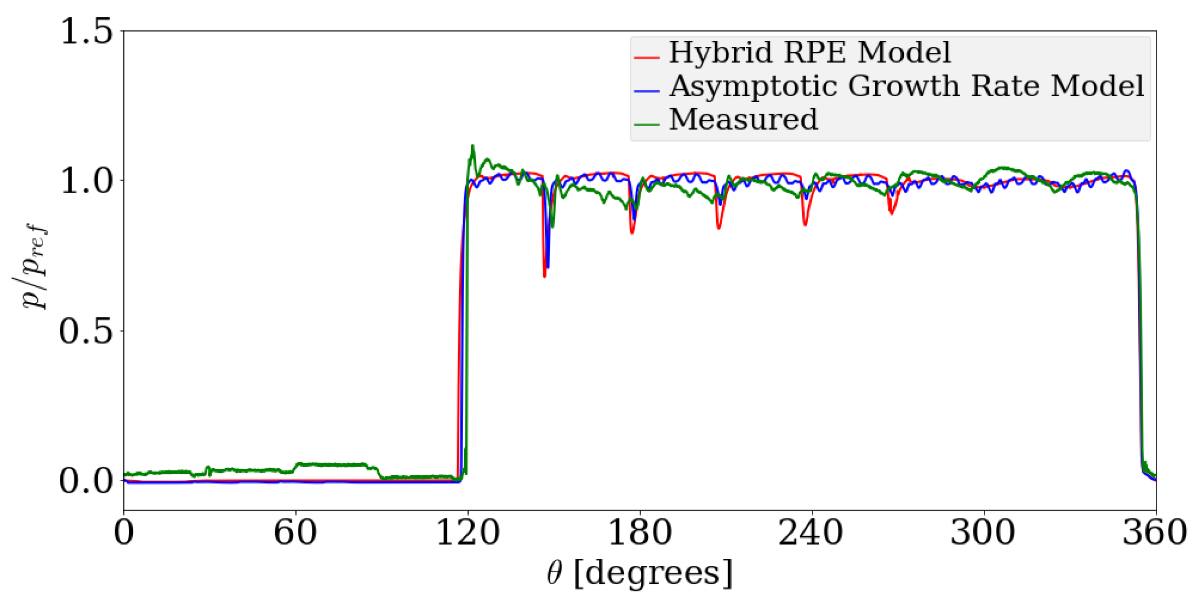
Moderate to extreme cavitation occurs for the case with an operating speed of 1500 rpm. The pressure at the inlet is significantly lower than the saturation pressure of the gas component. For this case, the pressure profiles may be seen to follow the experimental trends quite accurately. The same is observed for the pressure profiles obtained at the delivery side shown in Figure 19, Figure 20 and Figure 21. The case with operating speed of 2000 rpm also corresponds to extreme cavitation. In this case, the Hybrid RPE model predicts a more accurate TSV pressure profile compared with the Asymptotic Growth Rate model. The flow rate profile predicted by the Hybrid RPE model has high fluctuations compared with the Asymptotic Growth Rate model. This arises on account of the large fluctuations in the void fraction of the bubble observed in the Hybrid RPE approach. Overall, both of the dynamic models perform well in the prediction of the measurable quantities. As the model is based upon a lumped parameter approach, a sensitivity analysis with respect to the number of Control Volumes used is not needed and is reflected with the agreement between aforementioned simulation results and experiments as well as those in Refs. [12,18].
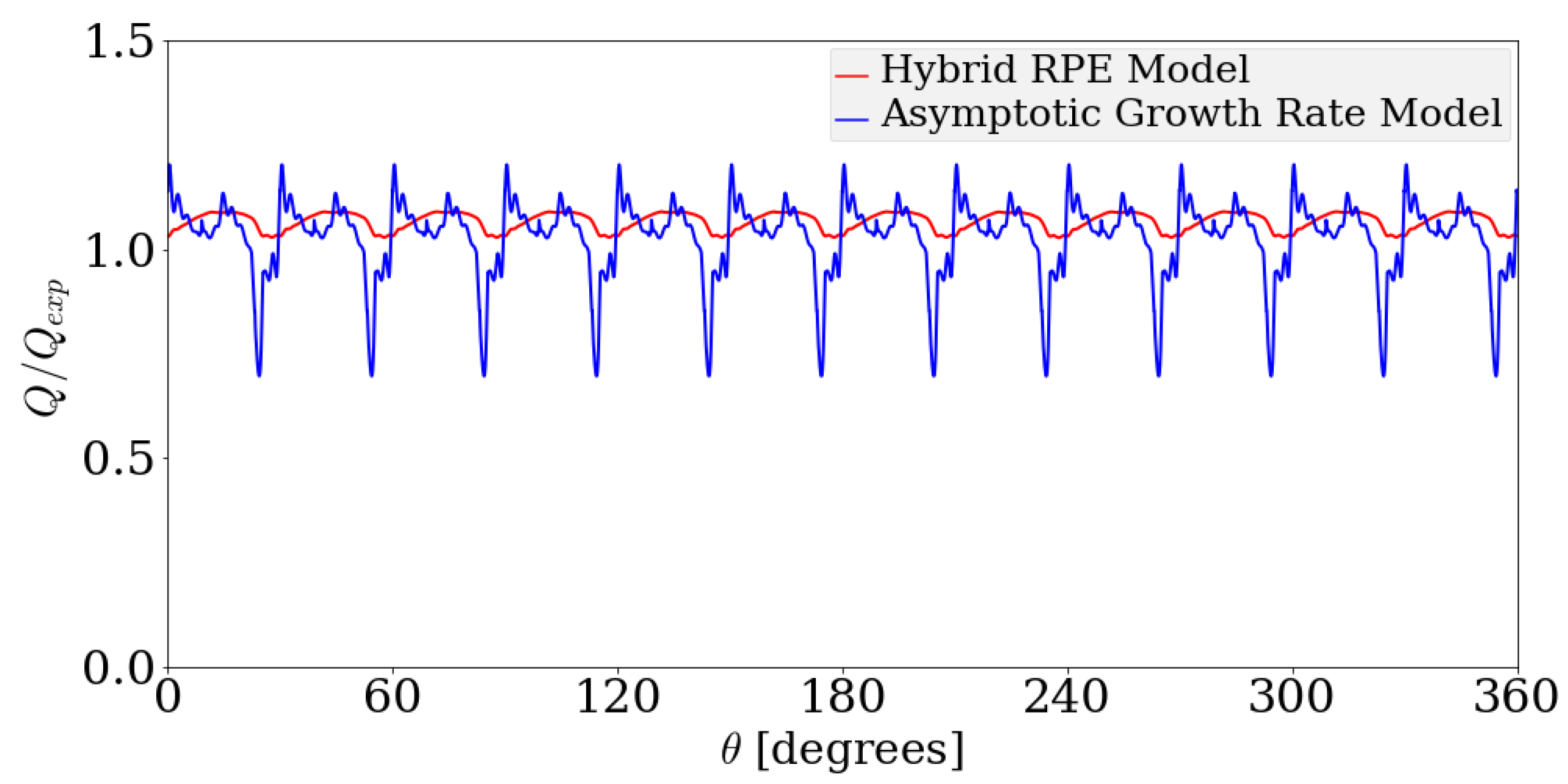
For each of the three cases shown before, the flow rates are computed and is shown in Figure 22. Strong variations appear in the flow rate simulated using the Asymptotic Growth Rate model, however, that modeled using the Hybrid RPE model appear consistent. In terms of the mean value of the flow rate, the Hybrid RPE model predicts the flow rate accurately.
8. Conclusions
The Hybrid Rayleigh–Plesset Equation model, a novel dynamic cavitation modeling approach, has been presented in this paper. The Hybrid RPE model is a high fidelity physically realizable model based on the implicit relationship between the radius of the bubble and the Energy of the system. The model solves the physics based RP equation to determine the timescales of bubble growth, condensation or dissolution and predicts the void fraction distribution accurately in a generic hydraulic system. The model introduces power law relationship to solve the RP equation in stiff regimes and has been demonstrated to predict the solution to the RP equation accurately. Furthermore, the model was implemented and applied to observe the dynamics of an External Gear Machine. The results predicted by the model were compared with the existing Asymptotic Growth Rate dynamic model and both the dynamic models are observed to reflect the experimental measurements accurately. The Hybrid RPE model overcomes the limitation of existing dynamic model with regard to the specification of empirically determined relaxation parameters and introduces dependence on the physically realizable parameters such as nuclei density and size in the hydraulic fluids. Thus, the Hybrid RPE model simulates the dynamics of a hydraulic system with a reduced set of physically realizable parameters. The predicting capabilities of this dynamic model would enable designs of External Gear Machines for optimized performance under cavitating conditions in future. In terms of model development, future work includes extension of the model to account for inhomogeneous nuclei distribution wherein bubbles of different radii are considered and bubble number density are considered within each CV and further validation of the modeled dynamics.
Author Contributions
Y.G.S., A.V. and S.D. conceived the modeling approach and designed numerical experiments and validated them at the Maha Fluid Power Research Center. All authors were involved in the analysis of data and the preparation of the manuscript.
Funding
This research received no external funding.
Acknowledgments
The authors would like to express their gratitude to Siemens (Munich, Germany) for the use of simulation software AMESim.
Conflicts of Interest
The authors declare no conflict of interest.
Nomenclature
| A | Cross sectional area of the orifice in a plane normal to the flow direction |
| a | Coefficient in power law relationship between dimensionless parameters |
| b | Exponent in power law relationship between dimensionless parameters |
| Width of a lateral gap | |
| Orifice coefficient | |
| c | Speed of sound |
| Saturated concentration of the incondensable gases | |
| E | Bulk modulus of a phase/mixture |
| Bulk modulus of the oil at a pressure | |
| Steady state energy of a fluid bubble system | |
| Total energy of a fluid bubble system | |
| f | Mass fraction of a phase |
| G | Contributions of energy from pressure and surface tension forces |
| H | Henry’s constant |
| h | Height of a lateral gap |
| k | Kinetic energy of the fluid |
| Gas release relaxation parameter | |
| Gas dissolution relaxation parameter | |
| Vapor evaporation relaxation parameter | |
| Vapor condensation relaxation parameter | |
| L | Length of a lateral gap |
| Number of outflow connections in ith chamber | |
| m | Mass of a phase/mixture |
| Number of inflow connections in ith chamber | |
| N | Bubble number density |
| p | Pressure in a control volume |
| Saturation pressure of the vapor component | |
| Saturation pressure of air | |
| Initial pressure | |
| Final pressure | |
| Pressure away from bubble interface | |
| Partial pressure of the gas in equilibrium | |
| Q | Volumetric flow rate through an orifice |
| Flow through the backflow groove | |
| Drain leakages | |
| Lateral leakages | |
| Radial leakages | |
| R | Bubble radius |
| t | Time |
| Dimensionless time | |
| T | Kinetic energy transported by the fluid |
| v | Flow velocity |
| V | Volume of a chamber/control volume |
| W | Work done per unit flow of mass |
Subscripts
| B | Bubble |
| g | Non condensable gas component |
| v | vapor phase |
| l | liquid phase |
| Summation indices | |
| inlet/inflow | |
| outlet/outflow | |
| Steady state |
Greek Symbols
| Void fraction | |
| Viscous dissipation rate | |
| Polytropic gas constant | |
| Dynamic viscosity | |
| Kinematic viscosity | |
| Density | |
| Coefficient of surface tension | |
| Angular position |
Abbreviations
| HYGESim | Hydraulic Gear Simulator |
| LHS | Left Hand Side |
| RHS | Right Hand Side |
| EGM | External Gear Machine |
| CV | Control Volume |
| TSV | Tooth Space Volume |
| RPE | Rayleigh–Plesset Equation |
| RP | Rayleigh–Plesset |
| RMS | Root Mean Squared |
| CFD | Computational Fluid Dynamics |
Appendix A. Derivation of the Compressible Orifice Equation
The compressible orifice equation Equation (11) can be derived beginning from the generalized formulation of the orifice equation obtained from the compressible form of the Bernoulli equation as:
In order to determine the flow rate in Equation (A1), the integral needs to be evaluated. The density of the homogeneous mixture can be expressed in terms of the mass fractions of individual components using Equations (6) and (8) as:
The integral can thus be written as:
Note that the integral is the boundary work done in compression or expansion of the fluid. As the gas and vapor components undergo polytropic processes, the density can be expressed for the gaseous phase as:
where are polytropic constants. On substituting the equation governing density, the following expression is obtained:
This term describes the work done in the compression and the expansion of the gas phase components in the fluid. For the liquid phase, the work term is evaluated using the definition of the bulk modulus:
With an exponential dependence of the bulk modulus on the pressure, the work term for the liquid phase () is evaluated as:
The compressible form of the orifice equation is finally obtained when the work terms are substituted:
References and Note
- Merkle, C.; Feng, J.; Buelow, P. Computational modeling of the dynamics of sheet cavitation. In Proceedings of the 3rd International Symposium on Cavitation, Grenoble, France, 7–10 April 1998; Volume 2, pp. 47–54. [Google Scholar]
- Zwart, P.; Gerber, A.; Belamri, T. A two-phase flow model for predicting cavitation dynamics. In Proceedings of the Fifth International Conference on Multiphase Flow, Yokohama, Japan, 30 May–4 June 2004; Volume 152. [Google Scholar]
- Schnerr, G.; Sauer, J. Physical and numerical modeling of unsteady cavitation dynamics. In Proceedings of the Fourth International Conference on Multiphase Flow, New Orleans, LA, USA, 27 May–1 June 2001; Volume 1. [Google Scholar]
- Dabiri, S.; Sirignano, W.; Joseph, D. A numerical study on the effects of cavitation on orifice flow. Phys. Fluids 2010, 22, 042102. [Google Scholar] [CrossRef]
- Dabiri, S.; Sirignano, W.; Joseph, D. Cavitation in an orifice flow. Phys. Fluids 2007, 19, 072112. [Google Scholar] [CrossRef] [Green Version]
- Dabiri, S.; Sirignano, W.; Joseph, D. Interaction between a cavitation bubble and shear flow. J. Fluid Mech. 2010, 651, 93–116. [Google Scholar] [CrossRef]
- Singhal, A.; Athavale, M.; Li, H.; Jiang, Y. Mathematical basis and validation of the full cavitation model. J. Fluids Eng. 2002, 124, 617–624. [Google Scholar] [CrossRef]
- Casoli, P.; Vacca, A.; Franzoni, G.; Berta, G. Modelling of fluid properties in hydraulic positive displacement machines. Simul. Model. Pract. Theory 2006, 14, 1059–1072. [Google Scholar] [CrossRef]
- SA Imagine HYD Advanced Fluid Properties, Technical bulletin 117. Technical report, 2016.
- Gholizadeh, H.; Burton, R.; Schoenau, G. Fluid bulk modulus: Comparison of low pressure models. Int. J. Fluid Power 2012, 13, 7–16. [Google Scholar] [CrossRef]
- Zhou, J.; Vacca, A.; Manhartsgruber, B. A novel approach for the prediction of dynamic features of air release and absorption in hydraulic oils. J. Fluids Eng. 2013, 135, 091305. [Google Scholar] [CrossRef]
- Zhou, J.; Vacca, A.; Casoli, P. A novel approach for predicting the operation of external gear pumps under cavitating conditions. J. Fluids Eng. 2014, 45, 35–49. [Google Scholar] [CrossRef]
- Shah, Y.G.; Vacca, A.; Dabiri, S.; Frosina, E. A fast lumped parameter approach for the prediction of both aeration and cavitation in Gerotor pumps. Meccanica 2018, 53, 175–191. [Google Scholar] [CrossRef]
- Manring, N. Hydraulic Control Systems; Wiley: Hoboken, NJ, USA, 2005. [Google Scholar]
- Blackburn, J. Fluid Power Control; Massachusetts Institute of Technology, The MIT Press: Cambridge, MA, USA, 1969. [Google Scholar]
- Merritt, H.E. Hydraulic Control Systems; John Wiley & Sons: Hoboken, NJ, USA, 1967. [Google Scholar]
- McCloy, D.; Martin, H. Control of Fluid Power: Analysis and Design; Chichester, Sussex, England, Ellis Horwood, Ltd.; Halsted Press: New York, NY, USA, 1980; 505p. [Google Scholar]
- Vacca, A.; Guidetti, M. Modelling and experimental validation of external spur gear machines for fluid power applications. J. Fluids Eng. 2011, 19, 2007–2031. [Google Scholar] [CrossRef]
- Vacca, A.; Dhar, S.; Opperwall, T. A coupled lumped parameter and CFD approach for modeling external gear machines. In Proceedings of the SICFP2011—The Twelfth Scandinavian International Conference on Fluid Power, Tampere, Finland, 18–20 May 2011; pp. 18–20. [Google Scholar]
- Dhar, S.; Vacca, A. A novel CFD–Axial motion coupled model for the axial balance of lateral bushings in external gear machines. Simul. Model. Pract. Theory 2012, 26, 60–76. [Google Scholar] [CrossRef]
- Dhar, S.; Vacca, A. A fluid structure interaction—EHD model of the lubricating gaps in external gear machines: Formulation and validation. Tribol. Int. 2013, 62, 78–90. [Google Scholar] [CrossRef]
- Rituraj, F.; Vacca, A. External gear pumps operating with non-Newtonian fluids: Modelling and experimental validation. Mech. Syst. Signal Process. 2018, 106, 284–302. [Google Scholar] [CrossRef]
- Vacca, A.; Franzoni, G.; Casoli, P. On the analysis of experimental data for external gear machines and their comparison with simulation results. In Proceedings of the ASME 2007 International Mechanical Engineering Congress and Exposition, Washington, CD, USA, 11–15 November 2007; American Society of Mechanical Engineers: New York, NY, USA; pp. 45–53. [Google Scholar]
- Shah, Y.G. Modeling and Simulation of Cavitation in Hydraulic Systems. Master’s Thesis, Purdue University, West Lafayette, IN, USA, 2017. [Google Scholar]
- Rayleigh, L. VIII. On the pressure developed in a liquid during the collapse of a spherical cavity. Philos. Mag. 1917, 34, 94–98. [Google Scholar] [CrossRef] [Green Version]
- Plesset, M. The dynamics of cavitation bubbles. J. Appl. Mech. 1949, 16, 277–282. [Google Scholar] [CrossRef]
- Brennen, C. Cavitation and Bubble Dynamics; Cambridge University Press: Cambridge, UK, 2013. [Google Scholar]
- Brennen, C. Hydrodynamics of Pumps; Cambridge University Press: Cambridge, UK, 2011. [Google Scholar]
- LSODA: ODEPACK Solver. Available online: http://people.sc.fsu.edu/ jburkardt/f77src/odepack/odepack.html (accessed on 1 June 2017).
- Vacca, A.; Casoli, P.; Greco, M. Experimental analysis of flow through external spur gear pumps. In Proceedings of the Seventh International Conference on Fluid Power Transmission and Control, Hangzhou, China, 7–10 April 2009. [Google Scholar]
- Greco, M.; Casoli, P.; Vacca, A. Experimental measurement and numerical simulation of ’inner-teeth space pressure’ in external gear pumps. In Proceedings of the 6th FPNI-PhD Symposium, West Lafayette, IN, USA, 15–19 June 2010. [Google Scholar]
Figure 1.
Schematic representation of the governing equations in the conventional lumped parameter approach: Pressure built up equation and the Orifice equations.
Figure 1.
Schematic representation of the governing equations in the conventional lumped parameter approach: Pressure built up equation and the Orifice equations.

Figure 2.
Structure of the simulation tool HYGESim [22].
Figure 2.
Structure of the simulation tool HYGESim [22].

Figure 3.
Schematic of a spherical bubble in an infinite fluid medium.

Figure 4.
Pressure variation (gage pressure) forced at a distance from a spherical bubble.

Figure 5.
Variation of the non-dimensionalized radius of a spherical bubble with initial radius m with parameters: m/s, kg/m, bar gage pressure, kg/s and m/s, subjected to forced pressure variation shown in Figure 4.
Figure 5.
Variation of the non-dimensionalized radius of a spherical bubble with initial radius m with parameters: m/s, kg/m, bar gage pressure, kg/s and m/s, subjected to forced pressure variation shown in Figure 4.

Figure 6.
Instantaneous and averaged radius of the bubble for a sudden pressure drop from initial pressure of 0 bar gage pressure to a final pressure of −0.7 bar gage pressure far away from the bubble interface with the parameters: m/s, kg/m, bar gage pressure, kg/s and m/s—(a) endpoints of the averaging interval (marked by solid points); (b) comparison between instantaneous and averaged radius.

Figure 7.
Variation of the Total Energy with time for a reference step pressure (Equation (24)) specified by and gage pressure with the same fluid properties as that chosen for the case shown in Figure 5.

Figure 8.
Variation of non-dimensional energy and energy dissipation rate for different values of while keeping constant: (a) variation of with non-dimensionalized time ; (b) variation of with non-dimensionalized time and (c) variation of with .
Figure 8.
Variation of non-dimensional energy and energy dissipation rate for different values of while keeping constant: (a) variation of with non-dimensionalized time ; (b) variation of with non-dimensionalized time and (c) variation of with .

Figure 9.
Variation of non-dimensional energy dissipation rate with dimensionless energy for (a) different values of while keeping constant and (b) different values of while keeping constant.
Figure 9.
Variation of non-dimensional energy dissipation rate with dimensionless energy for (a) different values of while keeping constant and (b) different values of while keeping constant.

Figure 10.
Comparison between the numerically computed solution to the Rayleigh–Plesset Equation and solution obtained using the proposed model with instantaneous non-dimensionalization parameters in (b), based on a forced linear pressure variation at a distance from the bubble interface shown in (a).

Figure 11.
Comparison between the numerically computed solution to the Rayleigh–Plesset Equation and solution obtained using the proposed model with instantaneous non-dimensionalization parameters in (b), based on a forced linear pressure variation at a distance from the bubble interface shown in (a).

Figure 12.
Simplified representation of the commercial EGM unit. The flow through the backflow groove, radial and lateral gaps are denoted, respectively, by .
Figure 12.
Simplified representation of the commercial EGM unit. The flow through the backflow groove, radial and lateral gaps are denoted, respectively, by .

Figure 13.
Simplified representation of an External Gear Machine along with the CVs and orifice connections.
Figure 13.
Simplified representation of an External Gear Machine along with the CVs and orifice connections.

Figure 14.
Scaled view of two of the TSVs corresponding to the drive gear in Figure 13 showing the radial leakage connections (), lateral leakage connection (), backflow groove connection () and drain leakage connection ().
Figure 14.
Scaled view of two of the TSVs corresponding to the drive gear in Figure 13 showing the radial leakage connections (), lateral leakage connection (), backflow groove connection () and drain leakage connection ().

Figure 15.
Experimental setup and its ISO schematic.

Figure 16.
Comparison between instantaneous TSV pressure profiles for the Asymptotic Growth Rate model, Hybrid Rayleigh–Plesset solution approach with experimental data for 1000 rpm speed and suction pressure of bar gauge pressure.
Figure 16.
Comparison between instantaneous TSV pressure profiles for the Asymptotic Growth Rate model, Hybrid Rayleigh–Plesset solution approach with experimental data for 1000 rpm speed and suction pressure of bar gauge pressure.

Figure 17.
Comparison between instantaneous TSV pressure profiles for the Asymptotic Growth Rate model, Hybrid Rayleigh–Plesset solution approach with experimental data for 1500 rpm speed and suction pressure of bar gauge pressure.
Figure 17.
Comparison between instantaneous TSV pressure profiles for the Asymptotic Growth Rate model, Hybrid Rayleigh–Plesset solution approach with experimental data for 1500 rpm speed and suction pressure of bar gauge pressure.

Figure 18.
Comparison between instantaneous TSV pressure profiles for the Asymptotic Growth Rate model, Hybrid Rayleigh–Plesset solution approach with experimental data for 2000 rpm speed and suction pressure of bar gauge pressure.
Figure 18.
Comparison between instantaneous TSV pressure profiles for the Asymptotic Growth Rate model, Hybrid Rayleigh–Plesset solution approach with experimental data for 2000 rpm speed and suction pressure of bar gauge pressure.

Figure 19.
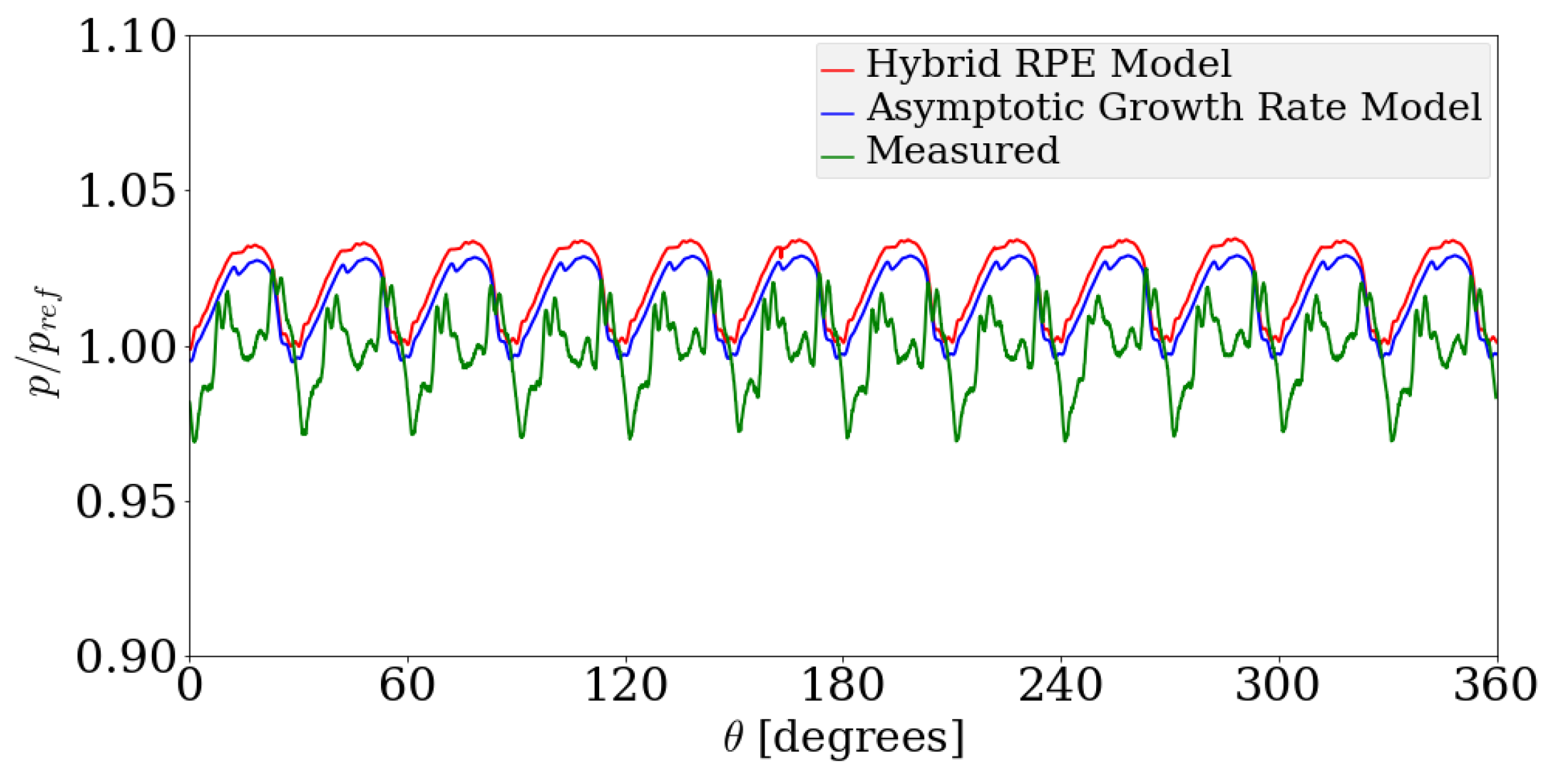
Comparison between delivery pressure ripple for the Asymptotic Growth Rate model, the Hybrid Rayleigh–Plesset Solution approach with experimental data, for an operating speed of 1000 rpm and a suction pressure of −0.06 bar gauge pressure. The modeled pressure fluctuations are within +3.5% and −0.2% while the measured data is within +2.5% and −3.1% of the reference value.
Figure 19.
Comparison between delivery pressure ripple for the Asymptotic Growth Rate model, the Hybrid Rayleigh–Plesset Solution approach with experimental data, for an operating speed of 1000 rpm and a suction pressure of −0.06 bar gauge pressure. The modeled pressure fluctuations are within +3.5% and −0.2% while the measured data is within +2.5% and −3.1% of the reference value.

Figure 20.
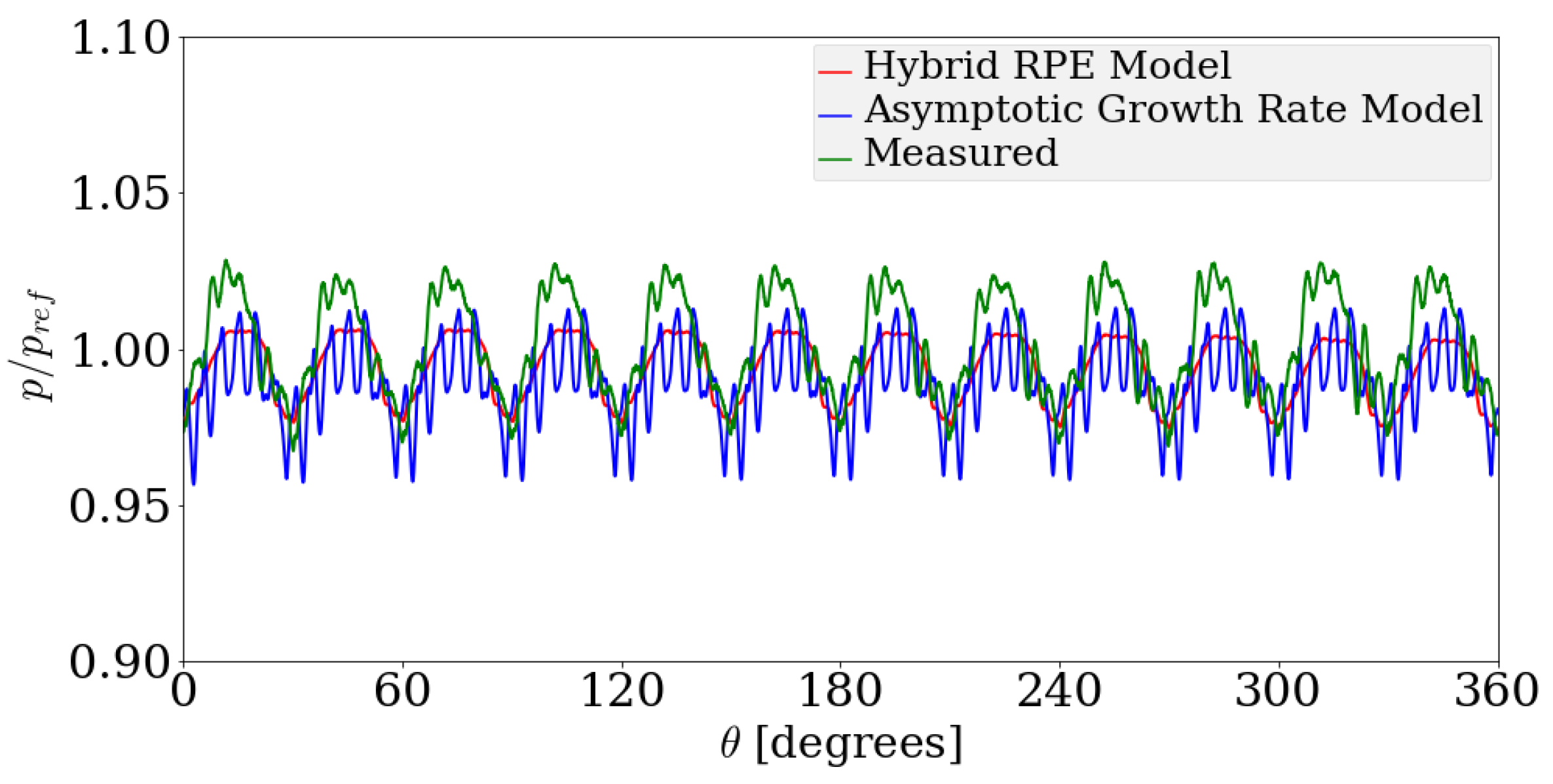
Comparison between delivery pressure ripple for the Asymptotic Growth Rate model, the Hybrid Rayleigh–Plesset Solution approach with experimental data, for an operating speed of 1500 rpm and a suction pressure of bar gauge pressure. The modeled pressure fluctuations are within +0.6% and −2.7% while the measured data is within +2.8% and −3.2% of the reference value.
Figure 20.
Comparison between delivery pressure ripple for the Asymptotic Growth Rate model, the Hybrid Rayleigh–Plesset Solution approach with experimental data, for an operating speed of 1500 rpm and a suction pressure of bar gauge pressure. The modeled pressure fluctuations are within +0.6% and −2.7% while the measured data is within +2.8% and −3.2% of the reference value.

Figure 21.
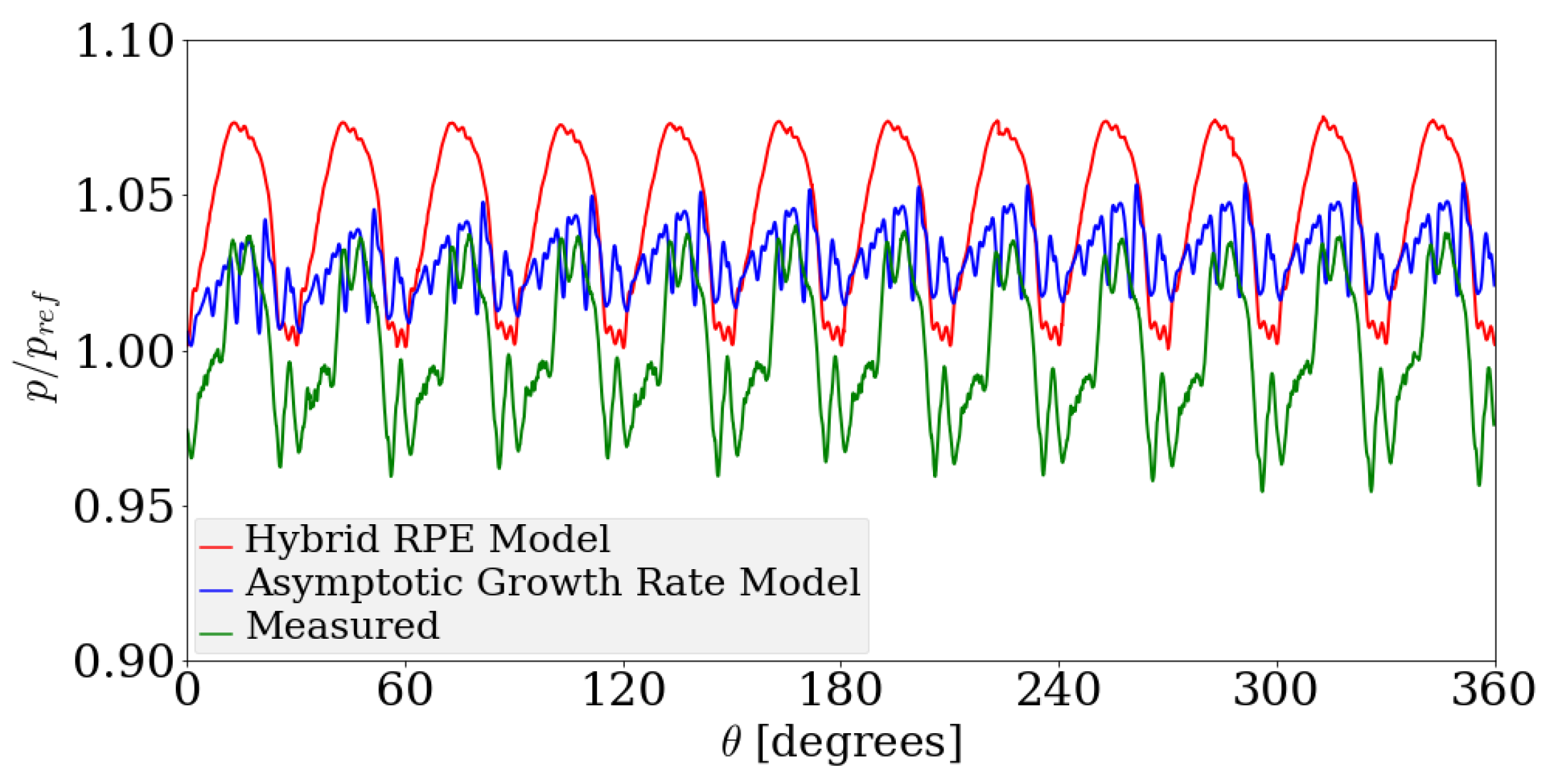
Comparison between delivery pressure ripple for the Asymptotic Growth Rate model, the Hybrid Rayleigh–Plesset Solution approach with experimental data, for an operating speed of 2000 rpm and a suction pressure of bar gauge pressure. The modeled pressure fluctuations are within +7.5% and −0.0% while the measured data is within +4.0% and −4.5% of the reference value.
Figure 21.
Comparison between delivery pressure ripple for the Asymptotic Growth Rate model, the Hybrid Rayleigh–Plesset Solution approach with experimental data, for an operating speed of 2000 rpm and a suction pressure of bar gauge pressure. The modeled pressure fluctuations are within +7.5% and −0.0% while the measured data is within +4.0% and −4.5% of the reference value.

Figure 22.
Comparison between delivery flow rates for the Asymptotic Growth Rate model and the Hybrid Rayleigh–Plesset Solution approach, for an operating speed of 1000 rpm.
Figure 22.
Comparison between delivery flow rates for the Asymptotic Growth Rate model and the Hybrid Rayleigh–Plesset Solution approach, for an operating speed of 1000 rpm.


Table 1.
Main specifications for the EGM unit.
| Feature | Description |
|---|---|
| Number of teeth | 12 |
| Displacement | 11.2 cc |
| Hydraulic oil | ISO VG 46 mineral oil |
| Suction pressure | <2 bar |
| Maximum pressure | 250 bar |
| Operating pressure | 500–2500 rpm |
Table 2.
Description of the sensors used in the experiment [12].
Table 2.
Description of the sensors used in the experiment [12].
| Sensor | Type | Manufacturer | Range | Accuracy (% F.S.) |
|---|---|---|---|---|
| T1 | Resistive | TERSID® (Milan, Italy) | (−50 °C, 200 °C) | 1.00% |
| P1, P3 | Strain gauge | WIKA® (Bavaria, Germany) | 0–40 bar | 0.25% |
| P2 | Strain gauge | WIKA® (Bavaria, Germany) | 0–400 bar | 0.25% |
| P4 | Piezoelectric | KISTLER® (Winterthur, Switzerland) | 0–1000 bar | 0.8% |
| (quartz, 140 kHz) | ||||
| P5 | Piezoresistive | ENTRAN® (Ludwigshafen, Germany) | 0–350 bar | 0.5% |
| (450 kHz) | ||||
| Q1 | Flow meter | VSE® (Neuenrade Germany) VS1 | 0.05–80 L/min | 0.3% measured value |
Table 3.
Mean flow rate comparison between the Hybrid Rayleigh–Plesset equation model and the Asymptotic Growth Rate model.
Table 3.
Mean flow rate comparison between the Hybrid Rayleigh–Plesset equation model and the Asymptotic Growth Rate model.
| Operating | Suction | Delivery | Hybrid RPE Model | Asymptotic Growth Rate |
|---|---|---|---|---|
| Speed (rpm) | Pressure (bar) | Pressure (bar) () | Flow Rate | Model Flow Rate () |
| 1000 | −0.06 | 100 | 1.06 | 1.03 |
| 1500 | −0.64 | 100 | 1.02 | 0.93 |
| 2000 | −0.72 | 150 | 1.0 | 1.0 |
© 2018 by the authors. Licensee MDPI, Basel, Switzerland. This article is an open access article distributed under the terms and conditions of the Creative Commons Attribution (CC BY) license (http://creativecommons.org/licenses/by/4.0/).
Share and Cite
MDPI and ACS Style
Shah, Y.G.; Vacca, A.; Dabiri, S. Air Release and Cavitation Modeling with a Lumped Parameter Approach Based on the Rayleigh–Plesset Equation: The Case of an External Gear Pump. Energies 2018, 11, 3472. https://doi.org/10.3390/en11123472
AMA Style
Shah YG, Vacca A, Dabiri S. Air Release and Cavitation Modeling with a Lumped Parameter Approach Based on the Rayleigh–Plesset Equation: The Case of an External Gear Pump. Energies. 2018; 11(12):3472. https://doi.org/10.3390/en11123472
Chicago/Turabian StyleShah, Yash Girish, Andrea Vacca, and Sadegh Dabiri. 2018. "Air Release and Cavitation Modeling with a Lumped Parameter Approach Based on the Rayleigh–Plesset Equation: The Case of an External Gear Pump" Energies 11, no. 12: 3472. https://doi.org/10.3390/en11123472
Note that from the first issue of 2016, this journal uses article numbers instead of page numbers. See further details here.