Comparison of Power Hardware-in-the-Loop Approaches for the Testing of Smart Grid Controls

Abstract

The fundamental changes in the energy sector, due to the rise of renewable energy resources and the possibilities of the digitalisation process, result in the demand for new methodologies for testing Smart Grid concepts and control strategies. Using the Power Hardware-in-the-Loop (PHIL) methodology is one of the key elements for such evaluations. PHIL and other in-the-loop concepts cannot be considered as plug’n’play and, for a wider adoption, the obstacles have to be reduced. This paper presents the comparison of two different setups for the evaluation of components and systems focused on undisturbed operational conditions. The first setup is a conventional PHIL setup and the second is a simplified setup based on a quasi-dynamic PHIL (QDPHIL) approach which involves fast and continuously steady state load flow calculations. A case study which analyses a simple superimposed voltage control algorithm gives an example for the actual usage of the quasi-dynamic setup. Furthermore, this article also provides a comparison and discussion of the achieved results with the two setups and it concludes with an outlook about further research.

1. Introduction

The energy system has become a fundamental pillar of our society and has to be changed dramatically. The Three Ds—Decarbonisation, Decentralisation and Digitalisation—headline the major requirements of Western society these days [1]. The ongoing process of climate change speeds up under ominous conditions. New research results of the Intergovernmental Panel on Climate Change strengthen assumptions of the negative effects on human society [2,3].These effects were provoked by the humanity itself by emitting carbon dioxide in large amounts from burning fossil resources (i.e., oil, gas, and coal). On 4 November 2016 in Paris, the world community committed to an agreement that will be keeping global temperature well below two degrees Celsius above pre-industrial level [4]. To achieve this goal, the entirety of human society will have to change their energy supply infrastructure to a renewable energy-based system.

The transition towards renewable energy and decentralised power supply leads to several challenges for the electrical grid operation, particularly on the distribution level [5,6]. Handling the large number of different characteristics of a fluctuating renewable generation and orchestrating the flexibility of decentralised loads and generation units in context of the distribution grids are complex challenges. To avoid potential problems in the distribution grid, such as voltage violations and line or power transformer overloading, Distribution System Operators (DSO) need to undertake smart operation and planning strategies, based on Information and Communication Technology (ICT) [7].

Examples and background to these ideas are given in [8,9,10,11] which supposedly will result in more resilient infrastructure [12,13] and are the context of various research projects [14,15,16,17]. This resulting change from capital expenditure- to operational expenditure-dominated grid operation should supposedly result in lower overall costs. This was also suggested by ref [18].

Digitalisation in a decentralised energy grid produces many data. This is what a complex ICT system is supposed to take care of. Taking into account that the energy grid is a sensitive system with massive consequences for society in case of a collapse, the ICT has to be tested in a save environment of a laboratory before deployment into the real world. Different test approaches have to be evaluated for specific use cases and boundaries [19]. The “Three Ds” will headline not only the major requirements for the transformation of the energy system, but also the motivation to develop the approach of this paper. To summarise, the question where the answers were sought for was: How can one test and validate systems which are performing a smart grid control strategy?

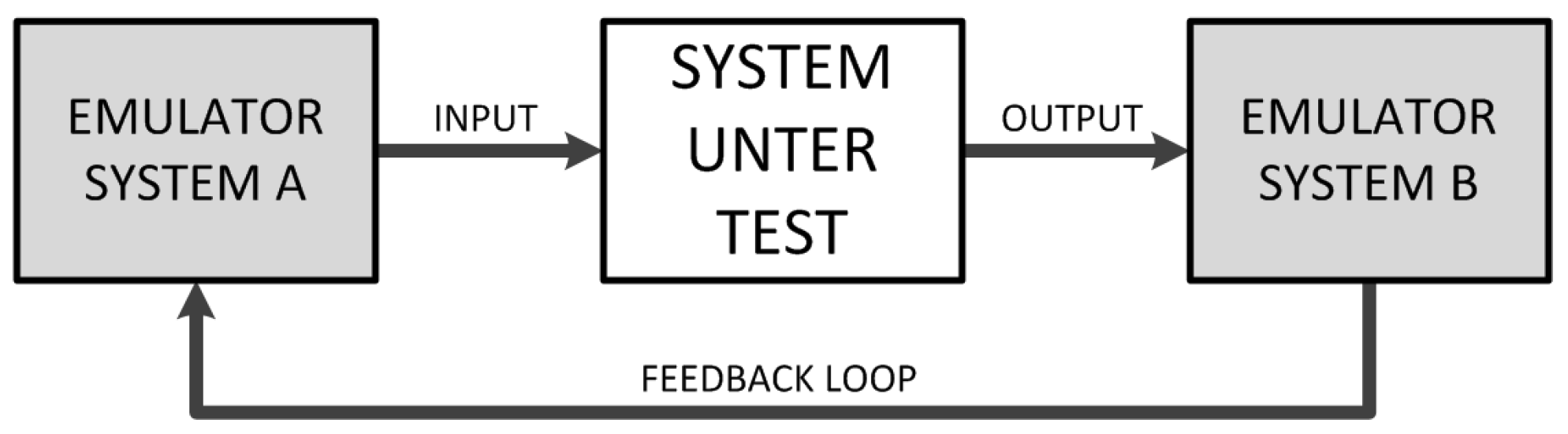
For the laboratory testing, one seeks for an environment with a variety of parameters to control. Such a setup can be described with the term of real-time Hardware-in-the-Loop (HIL) concepts [20,21,22]. The basic idea behind it is to place a system in an environment in which all inputs and outputs can be controlled. In general terms, this means that a test candidate (system, component or algorithm) is placed in an environment, where the adjacent systems are simulated, and the behaviour at the points of interface is emulated. Figure 1 depicts this approach in a generic way. Based on the reaction of the System-under-Test (SUT), the simulated environment adopts accordingly.

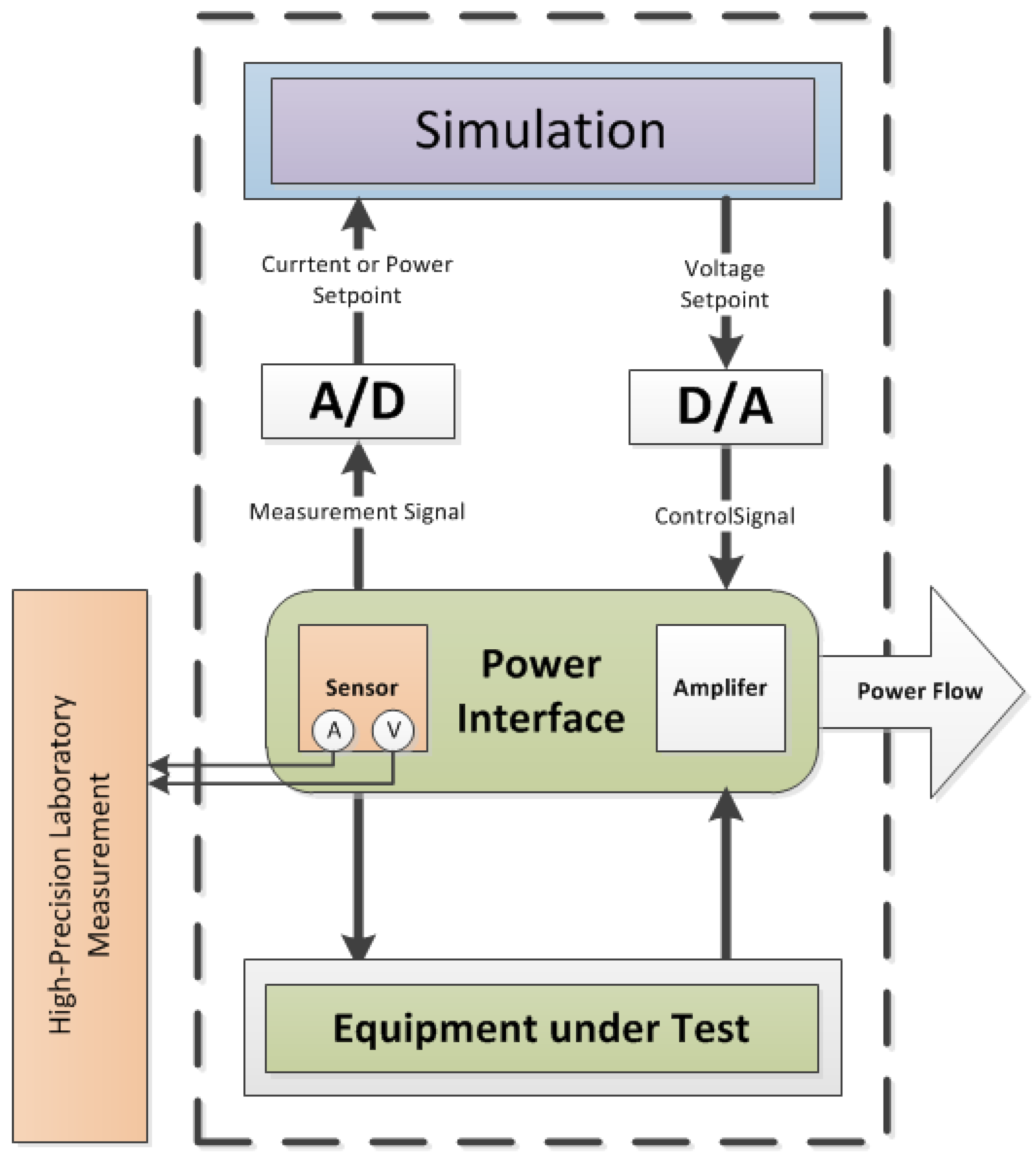
For the testing of power system components, an additional interface is necessary, i.e. the Power Interface (PI), as it can provide voltages (or currents) in the typical range of a power hardware device. Linear amplifier, switched-mode amplifier and coupled motor-generator assemblies are typically used [23,24]. In this article, two representatives from the switched-mode and linear amplifier category are utilised for the experiments. Beside the physical properties of the PI, the used Interface Algorithms (IA) are relevant for the success, as these algorithms deal with the occurring stability problems. This is discussed in detail in [25,26,27]. Combined with the issues regarding the stability of a PHIL experiment, as discussed in [26,27], such an experiment cannot be considered as plug’n’play. A simplification to enable a boarder range of research institutes to carry out PHIL experiments is the transition from PHIL to Quasi-Dynamic PHIL (QDPHIL). The main idea is to increase the time step which will enable the possibility to use steady state load flow simulation tools for the process. The typical temporal resolution of a PHIL experiment is in the range of 10–100 $\mathsf{\mu }$s [24], where, as with the implemented QDPHIL setup, a time step below one second is intended and realised. Through this simplification, the accuracy is supposedly reduced and the system setup needs to be analysed and the functionality validated.

This analysis is the scope of this paper. Details on the actual PHIL and QDPHIL setup used in this paper are given in Section 3. The transition from real-time calculation to steady state is discussed in more detail in Section 3.4. The QDPHIL concept will presumably enable the testing of superimposed control regimes as well as local control regimes such as a energy management systems. On the other hand, examples for topics which are in the scope examined with PHIL but not with QDPHIL experiments are given in [28,29,30]. All of the referenced experiments involve operation states which can be summarised as “disturbed operation”, whereas QDPHIL focuses on undisturbed operation. A detailed definition of requirements for the QDPHIL setup is given in Section 3.1. In [31], QDPHIL and quasi-static PHIL are mentioned as topics of current investigation.

The remaining part of this contribution is organised according to the following schema: In Section 2, a more detailed introduction to PHIL setups and smart grid testing in general is given. This includes the discussion of multi-domain Smart Grid testing and the application of the HIL concept to other domains such as ICT. The used PHIL and QDPHIL setups are introduced in Section 3. Section 4 describes the chosen validation methodology for comparing them. Section 5 presents the results of the carried out experiments and Section 6 describes the application of the proposed test methodology at the example of a case study. The results of the comparison are discussed in Section 7. Finally, this article is concluded by Section 8 with an outlook for further steps. The results of this paper are based on the work of the “Smart beats Copper” project within the ERIGrid Trans-national Access funding framework [32].

2. Overview of Validation Approaches of Smart Grid Systems

2.1. Testing Methodologies and Concepts in General

Testing such a complex system as described in the Introduction is often a challenging and complex task as it spans a diverse field of areas of investigation. These areas range from a single component test up to the test of a complete system [19]. As a second variation, the domain of test can vary as well and range from small scale systems in the premise of the costumer to medium or to large scale power plants. They can be communication tests, function testing for complex systems, or long-term stability evaluation. To structure these aspects, one can refer to the Smart Grid Architecture Model (SGAM) [33], which is structured in its layers (i.e., component, communication, data model, function and business), its domains (generation, transmission, distribution, DER (Distributed Energy Resources) and costumer premise) and its zones (i.e., process, field, station, operation, enterprise and market). For each layer, a variety of examinations can be undertaken. Therefore, the object under investigation can range from components to complex systems.

For a complex system, such as smart grids, a multiple stage approach is advisable. These stages can be generalised in the following five categories which consecutively build upon each step. These processes are based on the suggestions in [19,34]:

• Simulation-based Test: Small-scale to large-scale tests of concepts in a simulated environment during an early phase of the development.
• Controller Target Test: Small-scale test with the control functions implemented on the actual target.
• Laboratory Test: Small-scale test with a limited number of components in a controlled environment. Complexity reaches from basic component tests up to complex system tests.
• Pilot Test: Small-scale test with a limited amount of components in an uncontrolled environment to evaluate the difficulty of a real-world application. Typically, up to medium complexity functions are tested.
• Field Test: Medium-scale test with a few hundred up to a few thousand components in a real environment for preparing a large scale implementation of the tested system.

2.2. Introduction to PHIL

A typical PHIL setup consists of three main parts, that are depicted in Figure 2 and described hereafter: the SUT, the PI and the Simulation Module [20,21,22,25,26]:

• System-under-Test (may also be referred to as Hardware-under-Test (HUT), Device-under-Test (DUT) or Equipment-under-Test (EUT)): In the domain of smart grids, it is typically some kind of generation or consumption unit whose properties or functions are the subject of the examination. Around this element the PHIL systems are set up.
• Power Interface: Provides the ability to set the operating points for the real electrical system (e.g., voltage). There are basically three main types of PI: linear power amplifier, switched-mode power amplifier and generator based PI [23,24]. The dependent parameters need to be measured and are fed back as analogue signals or digital values into the simulation process. Furthermore, a system setup can be distinguished by the set output variable of the PI, which can be either voltage or current [23]. The feedback of the measured values forms a closed-loop to synchronise the HIL simulations and SIL simulations, whereas in open-loop tests a feedback of the measurements is not part of the system setups.
• Simulation Module: The simulation system—usually a Digital Real-Time Simulator (DRTS)—receives the measured values and calculates new set points, which are sent to the power interface as analogue signals or digital values based on the type of the power interface. The simulation tools are distinguished by their calculation method. Typical methods are transient calculation, phasor calculation or steady state calculation. Besides the different methodologies of the simulation, the used IA is of particular importance. An overview of the different concepts and corresponding algorithms is given in [23,26,27].

Details on the possibilities for the calculation methodologies are given in

Table 1. Comparison of different methods for the calculation of energy transfer and control processes.

Name	Description	References
Transient Calculation	Besides the fundamental frequency, all transient components of the input signals are used for the calculation of the voltage signals. This is also considered as electromagnetic transient (EMT) simulation.	([35], Ch. 13) [36,37]
Phasor Calculation Fundamental Frequency	In contrast to the transient calculation, one special case is considering only the fundamental fractions of the analogue input signals. In the context of PHIL, this can be used to ensure that SUT is operated under conditions with good properties in respect to power quality issues.	[37]
Effective Value Calculation	The effective value calculation method only considers the effective value of the input signals, which is typically used for steady state simulation. This is also illustrated as root mean square.	[37,38]

.

2.3. Smart Grid Testing and Usage of Additional X-in-the-Loop Concepts

Besides the PHIL concepts, there are further domains which can be simulated and controlled relevant for a holistic system testing of a smart grid strategy. They are listed and explained in

Table 2. Comparison of different domains using the X-in-the-loop concept for system testing with focus on the energy sector.

Name	Description	References
Hardware-in-the-Loop (HIL)	The subject of the system testing can be any physical component that can provide small scale input and output signals. HIL can also be seen as general term and can be specified by the following test categories	[21,22]
Software-in-the-Loop (SIL)	Software components are the subject of a SIL test setup. The input and output signals are the calls and responses of the adjacent software components that are emulated.	[39]
Controller Hardware-in-the-Loop (CHIL)	Subjects are the controller boards of a power hardware device. A CHIL setup will therefore simulate the mechanical, electrical and power electronic parts of the power hardware device, which are controlled by the tested controller board. In contrast to a PHIL-setup, the controller board is introduced to the small signals which are typically provided by the power hardware. The reaction of the controller board to a disturbance can be examined and resulting voltages and currents can be evaluated regarding the relevant specification. CHIL tests are typically undertaken before lab testing of the complete device.	[22]
Power Hardware-in-the-Loop (PHIL)	The subject of this system is a component from the power system domain. In contrast to HIL, the input and output signals can be typical power systems levels, e.g., a common low-voltage connection with 400 $V_{AC}$ and up to a nominal power of 1 MVA.	[20,21,22]
ICT Hardware-in-the-Loop (ICTHIL)	A complex smart grid system is typically based on communication and relies on package-based communication connection like IP/TCP or UDP, which often suffers from impairments like latency, package drop, package reorder or corruption of data in real-world applications. This means that, when testing a system, these effects have to be reproduced as well. Therefore, it is, e.g., necessary to precisely weaken the transmission path. This effect can be achieved by using a physical network emulator. If the communication network is simulated as well, the term Network-Simulation-in-the-Loop (NSIL) can be used.	[39,40,41]

. As the discussion of the trends in the previous section has shown, digitalisation is one of the key elements for future system design. When setting up a test environment for smart grid control strategies, communication components and communication protocols are as important as the actual electrical grid properties. Considering these aspects, the concept depicted in Figure 3 was developed and used in the case study discussed in Section 6. The experiment combined the implemented QDPHIL setup as well as SIL and ICT Hardware-in-the-Loop (ICTHIL) aspects for the test of a superimposed voltage control. This experiments gives a practical example for the use of QDPHIL system setup.

3. Proposed System Setup

This section starts with the description of the requirements for the QDPHIL setup and the two implemented system setups which are compared in this contribution. This section is concluded with a discussion of the difference of phasor calculation use in an PHIL setup and the steady state calculation of the QDPHIL Setup.

3.1. Requirements for the Proposed Use

The planned use of a switched-mode PI as key component is for system testings of complex smart grid systems. The PI is available in both institutions involved in this contribution. The primary use of these PI are system function testings with a given test profile of the voltage which involves voltage swell, Q(U)-control, etc. It is suggested that the PI can also be used in a QDPHIL setup as described in the previous section, when the main goal is to analyse the system behaviour and not to focus on the dynamic behaviour of a single component involved. Regarding the set point of the PI of the PHIL and GDPHIL experiments, the setups were only designed for voltage set points, consequently only current and power, can be used as feedback signal. Systems that are in the scope of the test environment feature at least one of the characteristics stated in

Table 3. Overview of the requirements for the proposed use.

Category	Domain	Requirement
Systems Properties	Involved Domains	SGAM Domain Distribution, Decentralised Energy Resource or Customer Premise
	Communication	communication over WAN (e.g., BPL or Mobil 4G)
	Communication	multiple communication protocols are used and converter
	Control	central and decentralised control
	Control	autonomous or partially autonomous control of multiple systems
	Timing	update and control cycles > 30 s
Requirements	Timing	PHIL cycle time $t_{PHIL}\le 1\mathrm{s}$
	Accuracy	only sinusoidal waveform
	Accuracy	low voltage deviation $\mathsf{\Delta }U\le 1V_{RMS}$
	Operation Mode	only voltage type interface algorithm

. Based on the characterisation of the tested systems, the requirements for QDPHIL setup are stated in the lower part of the table.

3.2. PHIL System Setup A: Opal-RT RT-LAB with Spitzenberger Spies PAS

The system analysed first was based on a linear signal amplifier (i.e., Spitzenberger Spies PAS [42]) as power interface which simulates a grid connection point from the simulated grid. The PI receives an analogue voltage signal from the DRTS (i.e., Opal-RT [43]), which generates the signal according to the parameters of the simulated grid connection point (e.g., voltage $U_{pcc}$). These parameters are calculated within a real-time dynamic simulation with a high-time resolution of typically 10–50 $\mathsf{\mu }$s, based on a code-generated model converted from a MATLAB/Simulink model. To close the simulation loop, the DRTS is fed back with analogue current measurements, which are converted internally to digital values to be entered into the simulation model. These transient measurements correspond to the feed-in power of the PV inverter (i.e., EUT: Fronius PV inverter, [44]), which is connected physically to the power interface representing the Point of Common Coupling (PCC) of the grid. As the IA for the setup, a voltage type Interface utilising an Ideal Transformer Model (ITM) [23] was selected. For the purpose of recording the simulation results, an external measurement system was connected to the PCC (cf. [45]). The described system is illustrated schematically in Figure 4 along with the second setup, which is discussed in the following section. In the course of the following sections, this setup is referred to as System Setup A.

3.3. QDPHIL System Setup B: Digsilent PowerFactory 2018 with Regatron TC.ACS

This setup proposes the utilisation of the steady-state load flow calculation of the power system analysis software (i.e., DIgSILENT PowerFactory [46]). The calculated voltage value at a predefined bus bar in PowerFactory is passed as a new voltage set point to a PI, which in this case is a switched-mode voltage source from Regatron (i.e., Type: TC.ACS [47]). For sending the set values, an interface was programmed in C# language that utilises the API provided by the manufacturer to communicate with PI. A PV inverter (cf. [44]) is connected physically to the voltage source as EUT and feeds in power to the grid. The active and reactive power of the PV inverter is captured by a measurement device (cf. Janitza UMG96 [48]). The RMS measurements are fed back to the simulation in PowerFactory as digital values to form a closed loop. For this measurement feedback, an interface was programmed in Python utilising Modbus/TCP functionality of the measurement device. The system setup is illustrated schematically in Figure 4. To control the voltage in the simulation of PowerFactory, an external function was programmed in Python. To control the voltage in the steady state load flow calculations of PowerFactory, another external Python function was developed for the control and synchronisation of these calculations. In the course of the following sections, this setup is referred to as System Setup B.

3.4. Discussion of the Mathematical Difference of PHIL System A and QDPHIL System B

The used steady state simulation approach in System Setup B differs significantly from the phasor calculation used in the Opal-RT system of System Setup A, especially when comparing the cycle times. Regarding the calculation time, a transient PHIL simulation setup should achieve around a couple of microseconds. For System Setup B, an approximately 400 ms calculation time was realised in the laboratory experiments. This difference in calculation method is described in the expression below, where the left part represents the instantaneous value of the voltage and the right part represents the steady state value of voltage:

$$u_{grid}\left(dt\right)\to U_{grid,RMS}\left(\mathsf{\Delta }t\right)$$

(1)

where $dt$ is typically 10–40 $\mathsf{\mu }$s, and $\mathsf{\Delta }t$ is approximately 400 ms. The second proposed method could be named as the Quasi-Static Power-Hardware-in-the-Loop [31] in contrast to the classical PHIL setup which can be referred to as Real-Time Power-Hardware-in-the-Loop. Depending on the purpose of the examinations, which could correspond to the described requirements (cf. Section 3.1), the use of the Quasi-Static PHIL could be advisable.

3.4.1. Phasor Calculation

The mathematical equations to describe the used voltage step for evaluation of the system setups are presented in this section. For a modelled grid with a slack node and a single impedance between the slack node and the point of common coupling, the voltage at the PCC can be expressed in a simplified manner as addition of the voltage at the slack node and the voltage rise due to the power feed-in of the inverter over the impedance. To comply with the test procedure, as described in the following section (please refer to Section 4.1), a step function in the slack element was assumed. For the phaser calculation used in System Setup A, this relates to the following equations for each of the three phases:

$$\left(\begin{array}{c}{u}_{AN,PCC}\left(dt\right)\\ u_{BN,PCC}\left(dt\right)\\ u_{CN,PCC}\left(dt\right)\end{array}\right)=\left(\begin{array}{c}{u}_{AN,Slack}\left(dt\right)\\ u_{BN,Slack}\left(dt\right)\\ u_{CN,Slack}\left(dt\right)\end{array}\right)+\left(\begin{array}{c}▵u_{AN}\left(dt\right)\\ ▵u_{BN}\left(dt\right)\\ ▵u_{CN}\left(dt\right)\end{array}\right)$$

(2)

with a sinusoidal voltage source at a fixed frequency and a fixed phase angle deference $\theta$ of $\pm {120}^{\circ }$

$$\begin{array}{c}{u}_{AN,PCC}\left(t\right)=U_{nom}\times k_{step}\times \sin (2\times \pi \times f_{nom}\times t+{\theta }_{AN})\\ u_{BN,PCC}\left(t\right)=U_{nom}\times k_{step}\times \sin (2\times \pi \times f_{nom}\times t+{\theta }_{BN})\\ u_{CN,PCC}\left(t\right)=U_{nom}\times k_{step}\times \sin (2\times \pi \times f_{nom}\times t+{\theta }_{CN})\end{array}$$

(3)

The assumed step can be expressed with the help of a multiplier $k_{step}$ which changes its value depending on the calculation time. In this case, a change at the relative time t = 10 ms is used.

$$k_{step}\left\{\begin{array}{cc}1.04\hfill & t\le 10\mathrm{ms}\hfill \\ 1.08\hfill & t>10\mathrm{ms}\hfill \end{array}\right.$$

(4)

The voltage raise due to impedance can be determined by the following equation. In the phasor calculation, the actual value of the current is used for the calculation.

$$\begin{array}{c}▵u_{AN}\left(t\right)=Z_{grid}\times i_{AN}\left(t\right)=(R_{grid}+j\times X_{grid})\times \sin (2\times \pi \times f_{nom}\times t+{\theta }_{AN}+\cos {\left(\varphi \right)}_{load})\\ ▵u_{BN}\left(t\right)=Z_{grid}\times i_{BN}\left(t\right)=(R_{grid}+j\times X_{grid})\times \sin (2\times \pi \times f_{nom}\times t+{\theta }_{AN}+\cos {\left(\varphi \right)}_{load})\\ ▵u_{CN}\left(t\right)=Z_{grid}\times i_{CN}\left(t\right)=(R_{grid}+j\times X_{grid})\times \sin (2\times \pi \times f_{nom}\times t+{\theta }_{AN}+\cos {\left(\varphi \right)}_{load})\end{array}$$

(5)

3.4.2. Steady State Calculation

The steady state calculation can be carried out symmetrically. The used PI, the measurement device and the simulation program can also calculate the voltage in an unsymmetrical manner. Therefore, the equation changes to the examination of RMS values. The calculation methodology was adapted from [49].

$$U_{RMS,PCC}\left(t\right)=U_{RMS,Slack}\left(t\right)+▵U_{RMS,GRID}$$

(6)

Containing the slack voltage defined as step function with the same limits as the multiplier $k_{step}$ for the phaser calculation:

$$U_{RMS,Slack}\left(t\right)\left\{\begin{array}{cc}1.04p.u.\times U_{nom}\hfill & t\le 10\mathrm{ms}\hfill \\ 1.08p.u.\times U_{nom}\hfill & t>10\mathrm{ms}\hfill \end{array}\right.$$

(7)

The additional voltage needed to transfer power over the line segment is represented with the following equation. The variables change from a current to an active/reactive power.

$$▵U_{RMS,GRID}(P_{PCC}\left(t\right),Q_{PCC}\left(t\right))=\frac{P_{PCC}\left(t\right)\times R_{grid}+Q_{PCC}\left(t\right)\times X_{grid}}{U_{nom}}$$

(8)

3.4.3. Comparison of Phasor and Steady State calculation

A more detailed look into that context is provided in Figure 5 which depicts a constant voltage rise from 180 $V_{RMS}$ to 240 $V_{RMS}$. The ideal result is drawn as the blue dashed line. The behaviour of System Setup A is depicted as a stem diagram, where each stem represents a new set-point for the amplifier part of the power interface. The actual limit for the minimum step size is significantly lower than it is depicted in the diagram. The used step size is chosen for representation purpose. Each of these set points shows the result of a new calculation. In contrast to the small time steps of System Setup A, System Setup B sends RMS-set points to the PI with a bigger cycling time. This is depicted as the red line. The change from one set point to the next is one step, as illustrated. This is discussed with measured signals in the following section. These properties are only observed for the used system. Other systems have not been tested regarding this behaviour.

4. Validation Methodology

This article focuses on the comparison of the two system setups as introduced in Section 3. It is proposed that both systems can be used to evaluate the performance of smart grid components, solutions, and technologies as well as new approaches with high renewable energy feed-in if the requirements in Section 3.1 are met. For the validation of the QDPHIL setup, a two-stage process was chosen. In the first phase, the proposed system setup was tested and compared against the PHIL setup. Therefore, three test cases were used to characterise the differences in the response of the system to the test case scenarios. In the second phase, the QDPHIL system setup was used to conduct an experiment to gather results from a actual application of the QDPHIL concept. The results are presented in Section 6. A complex scenario was chosen which involves SIL components as well.

4.1. Test Methodology

The examination of both used system setups was carried out by comparing the response of the systems within three different scenarios. The scenarios reflect the most extreme possible variation as well as variations typically observed in real world test cases of the QDPHIL setup. The test cases are:

• Step Function: Voltage deviation at the slack bus bar from 1.04 p.u. to 1.08 p.u. in a step. This represents the most extreme change of a parameter in the modelled system. It was chosen to evaluate the difference in the dynamic behaviour of the systems in the time domain of seconds.
• Transient Behaviour of the Step Function: The voltage change of the two setups was evaluated regarding the transient behaviour of the system.
• Ramp Function: Voltage deviation at the slack bus bar from 1.04 p.u. to 1.08 p.u. as a voltage ramp over the course of 1–10 min. These are typical changes which were deployed to examine the stability of systems in varying conditions.

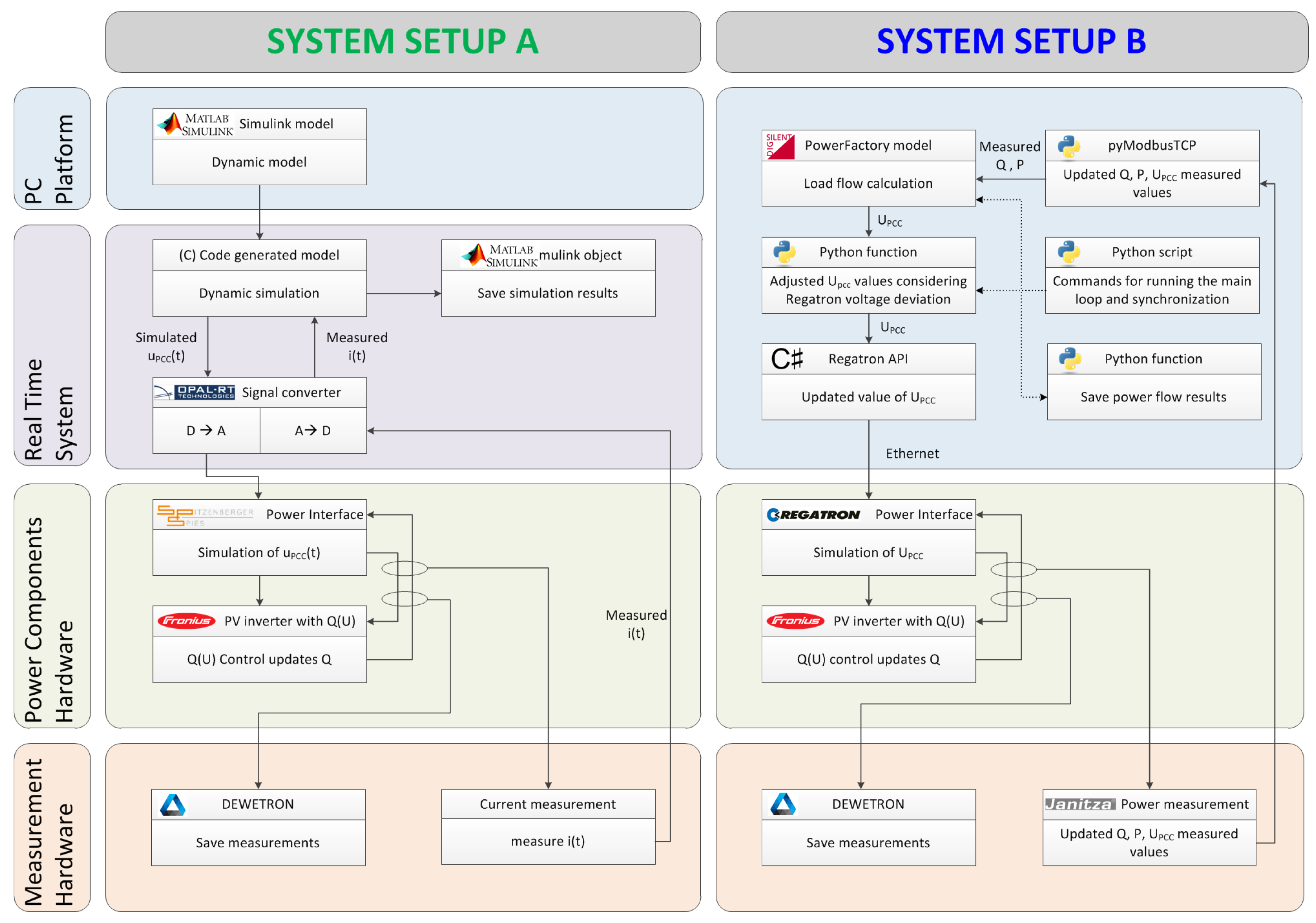
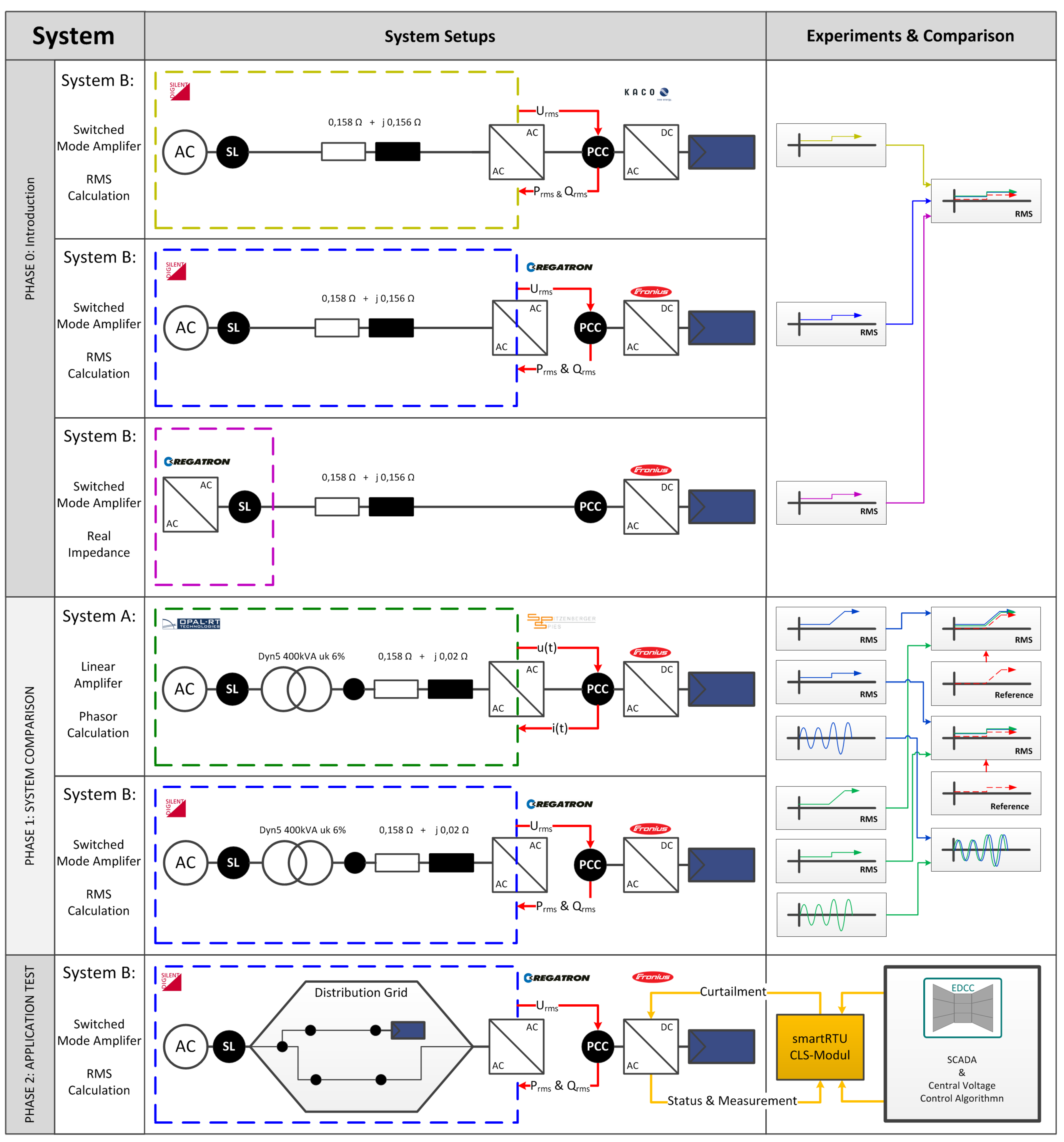
The individually used experiments are depicted in Figure 6 which also shows the system setups and the used grid model. The depicted experiments are grouped into three parts. These are the previous described tests for the comparison which are called Phase 1. Phase 1 is accompanied with a preliminary test to characterise the system setups, which is referred to as Phase 0. The subsequent tests are subject to a case study, which is called Phase 2 and is discussed in Section 6. These tests were also executed within the ERIGrid TA project “Smart beats Copper” at the host facility AIT in Vienna, Austria. Additional tests with System Setup B were executed at the Smart Grid Lab of Ulm University of Applied Sciences, Ulm, Germany.

4.2. Used Grid Model

The proposed system setups were investigated in Phase 1 when simulating a simplified grid model which consists of a regional Low-Voltage (LV) transformer, a power line represented as an impedance and a connection point (i.e., grid node), where a PV inverter is connected as depicted in Figure 6. It should be taken into consideration that the developed system can also be used for simulating large-scale grids, however, a simple grid was adopted for this study to avoid complexity in the simulation results.

4.3. Used EUT for the Test

The proposed system setups were tested considering a PV inverter as the EUT. Two inverters were used for the experiments, which was due to their availability at the different involved laboratories. The models Symo 20.0-3-M with nominal apparent power of 20 kVA and Symo 15.0-3-M with a nominal apparent power of 15 kVA from the manufacturer Fronius were used. 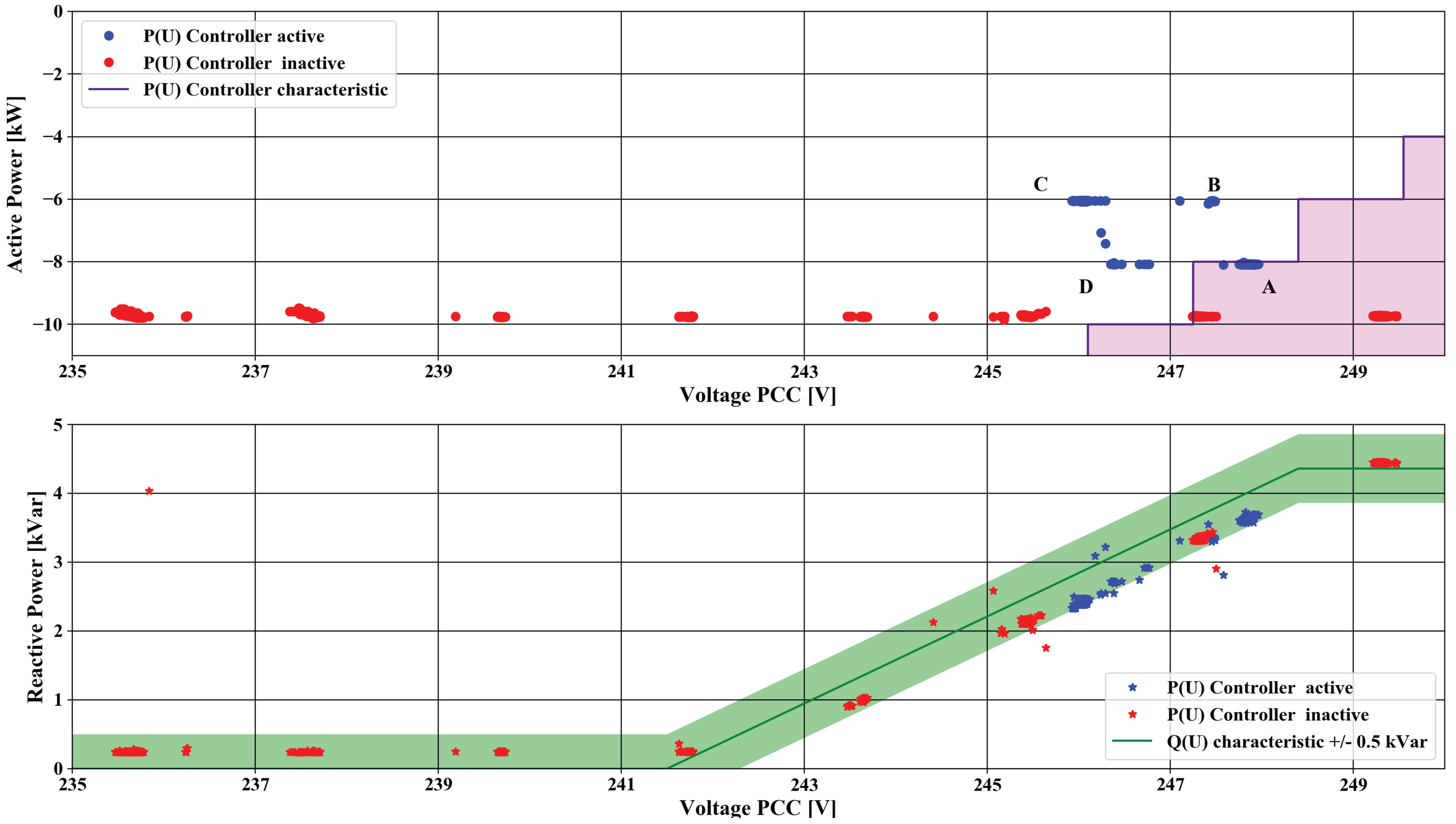Both systems originate from the same series and have the properties described in [44]. In addition, the function Q(U) for voltage control was configured in adaption to the suggestions by Elbs and Pardatscher [50] which again results in the parametrised Q(U) curve. Due to the reactive power priority of the implemented algorithm, the limit was lowered by 5% to prevent an oscillation of the controller. The selected set points are extreme scenarios as most of the relevant grid codes (e.g., [49,51]) or related documents rarely expect capabilities exceeding the limit of $cos\phi =0.9$ which corresponds to a limit of ±0.42 $Q/S_{nomm}$. The Q(U) controller has the option to set a time constant $T_C$. Different time constants were chosen. All chosen time constants represent challenging scenarios as the value suggested by the manufacturer is 5 s. An overview of the chosen parameters for the different tests is provided in

Table 4. Overview of the implemented step points parameterised for the system.

Parameter	Fronius Symo 20.0-3-M		Fronius Symo 15.0-3-M
	U (p.u.)	$\mathit{Q}/{\mathit{S}}_{\mathit{nomm}}$ (-)	U (p.u.)	$\mathit{Q}/{\mathit{S}}_{\mathit{nomm}}$ (-)
Setpoint 1	0.98	+1.00	0.98	+0.95
Setpoint 2	1.02	0.0	1.02	0.0
Setpoint 3	1.05	0.0	1.05	0.0
Setpoint 4	1.08	−1.00	1.08	−0.95
Time Constant $T_C$	10 ms		10 ms, 50 ms, 1 s

.

4.4. Used Test Scenarios for Phase 1

To examine the performance of the developed systems, two simulation scenarios were applied. In the first scenario, a voltage increase in single steps was implemented by means of increasing the set voltage in the slack bus bar. Such a scenario of voltage increase can be observed in practice, if a regional transformer changes the position of its On-Load Tap Changer (OLTC). In the second scenario, a gradual voltage increase in a ramp was implemented by means of increasing the set voltage in the slack bus bar. Such a scenario can be observed in practice if voltages in the medium-voltage grid increase according to natural increase of PV feed-in during a clear sky day.

5. Phases 0 and 1: Results of the Comparison of the System Properties of System Setup A and B

The comparison of the two system setups is the subject of this section. The preliminary tests of Phase 0 introduced the system properties. Section 5.2 and Section 5.3 discuss the transient and dynamic behaviour of the different systems setups when handling the voltage step. The discussion of the system behaviour for the modelled voltage ramp is given in the following section. The analysis of the cycles, especially of System Setup B, is outlined in Section 5.5. Section 7 concludes the Phases 1 and 2 discussion.

5.1. Introduction to the Compared Systems

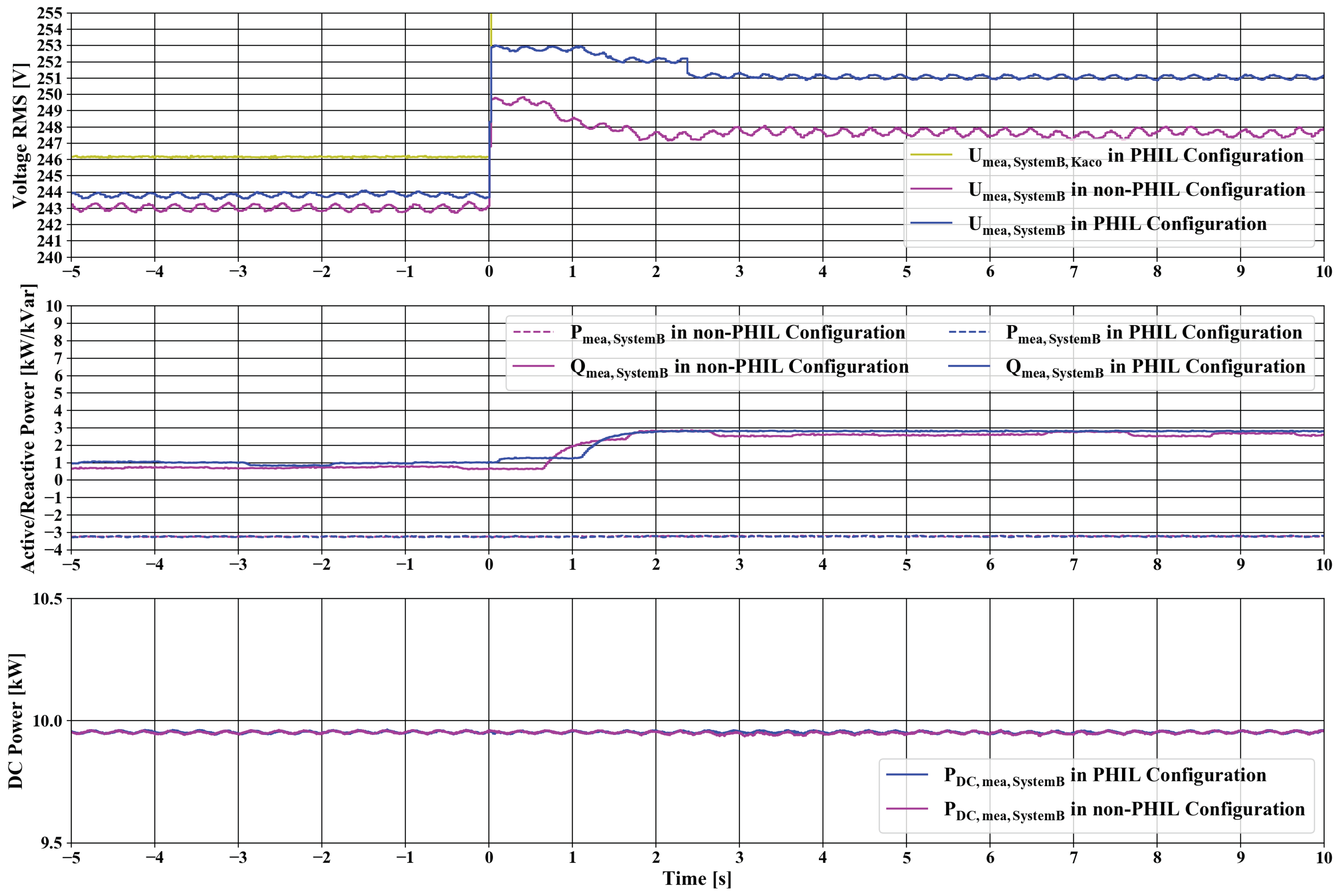
As a first step, a basic analysis of the behaviour of System Setup B is presented. The system was tested first with a non-PHIL configuration and a physical impedance between the PI and the EUT. In a next step, this was compared with the corresponding PHIL configuration. The impedance is typically used for flicker tests according to IEC 61000-3-3 [52], and is part of the SmartEST facility at AIT. As shown in Figure 7, an oscillation behaviour was present for both configurations. It was assumed that the oscillation was caused by the searching algorithm of Maximum Power Point Tracking (MPPT) of the Fronius PV inverter. For additional comparison, the pre-step part of a comparable setup with another type of inverter [53] is depicted. The voltage was more stable with this specific product in comparison to the results of the PV inverter. As this oscillation was caused by varying power in-feed, it was present in both configurations.

The difference between the two configurations could be seen most explicitly at the small voltage step of 2.5 s of the PHIL-configuration. Besides, a voltage deviation was present for both configurations. This offset ranged from approximately 1 $V_{RMS}$ to 3 $V_{RMS}$. Active and reactive power were fairly constant before and after the step which caused a change in reactive power due to the implemented Q(U)-control.

5.2. Comparison of the Transient System Response for Voltage Step

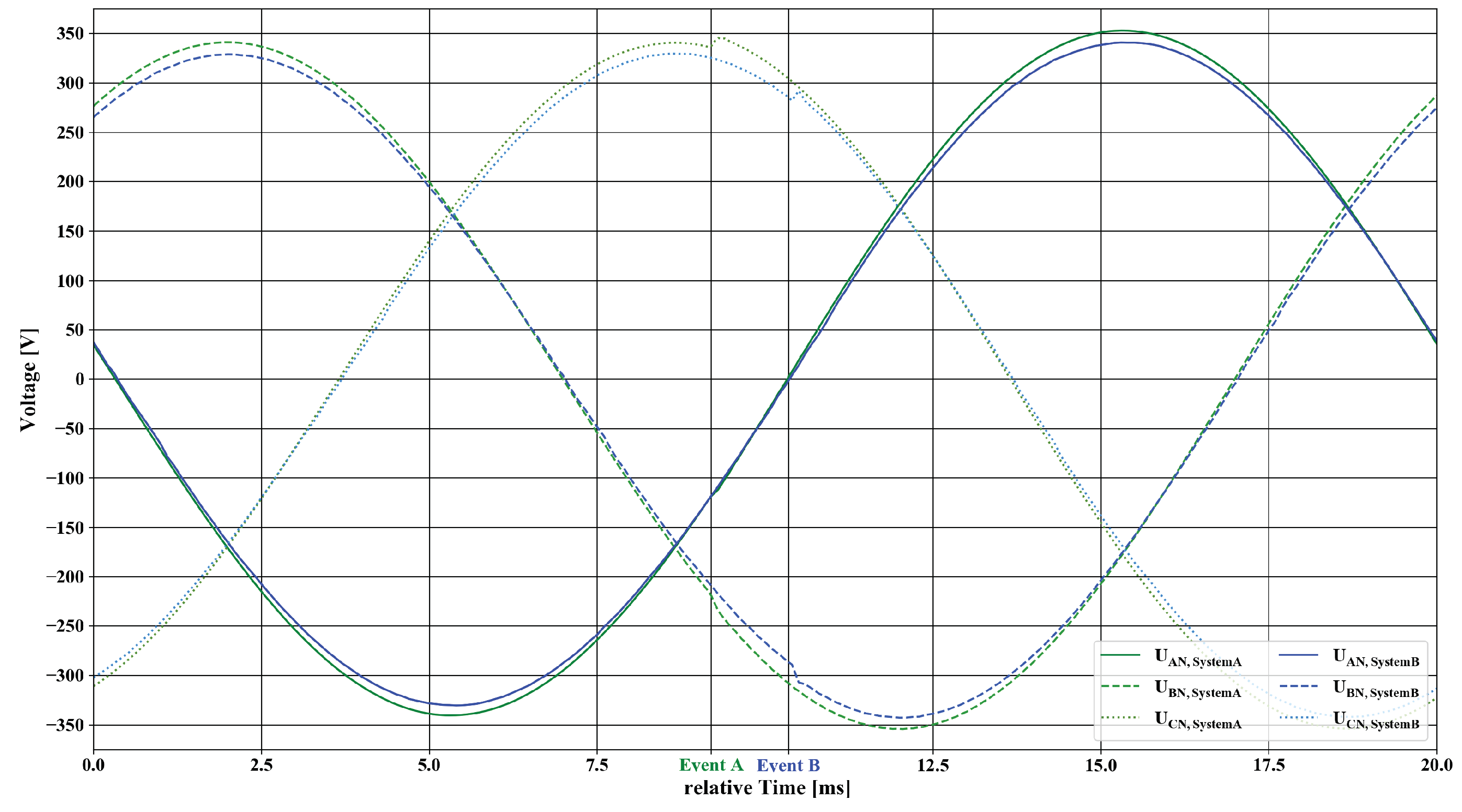
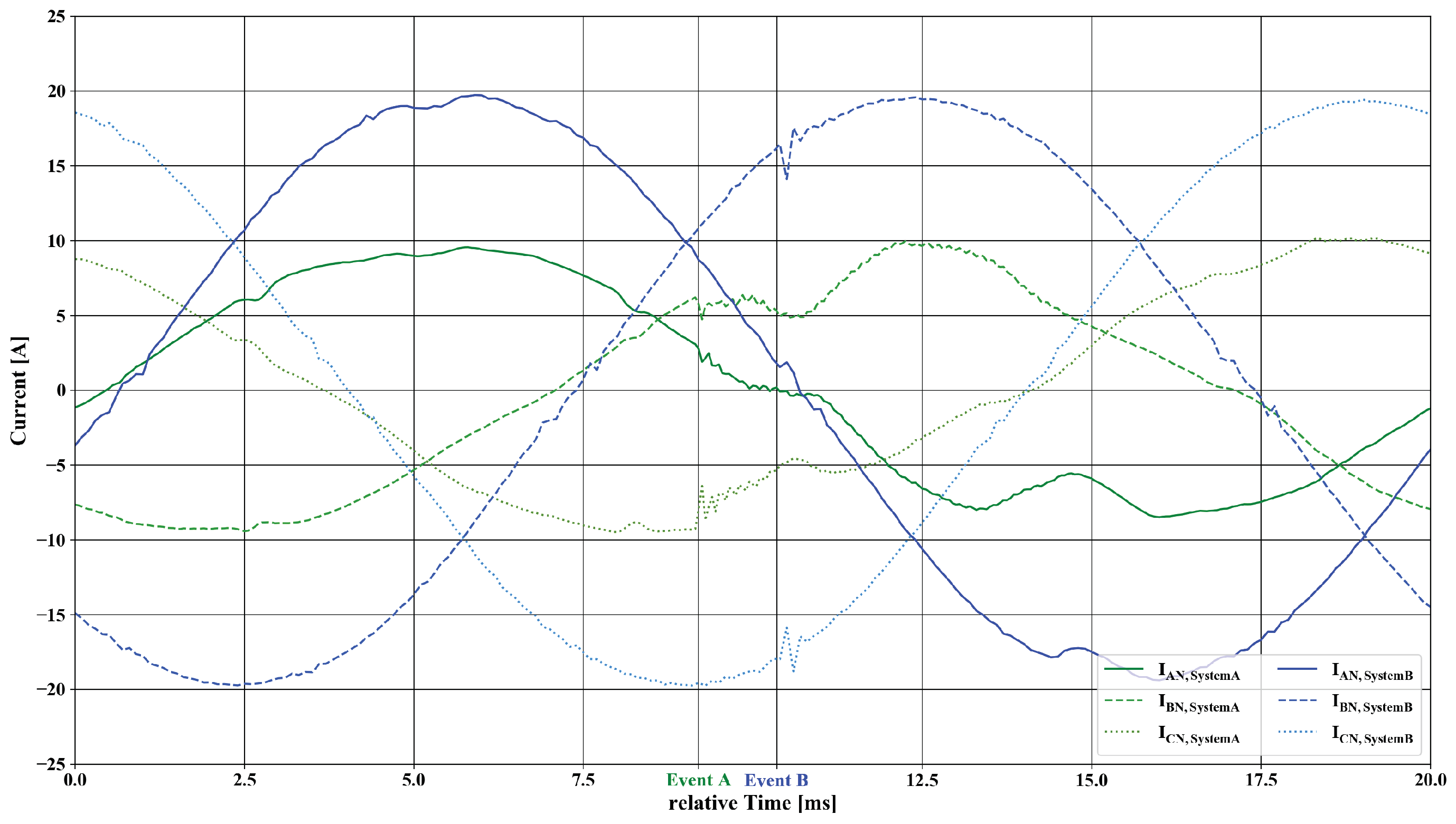
This section focuses on the comparison of the two setups described in Section 3.4. At first, the comparison of the used systems was made by analysing their transient behaviour. The trend of the voltage and the current of the two three-phase systems are depicted in Figure 8 and Figure 9, respectively. Both systems changed from one given waveform, which corresponded to a value of 240.6 $V_{RMS}$, to another waveform with a corresponding value of 249.7 $V_{RMS}$ and from 232.9 $V_{RMS}$ to 241.3 $V_{RMS}$ within roughly 100 $\mathsf{\mu }$s, respectively. For both systems, no lasting disturbance in waveform of the voltage could be observed. The given ideal sinusoidal waveform for the voltage was generated by both systems with neglectible fractions of no fundamental parts. The capabilities of both systems to generate a varying amount of non-fundamental disturbance have not been examined further in this contribution.

5.3. Comparison of the Dynamic System Response for Voltage Step

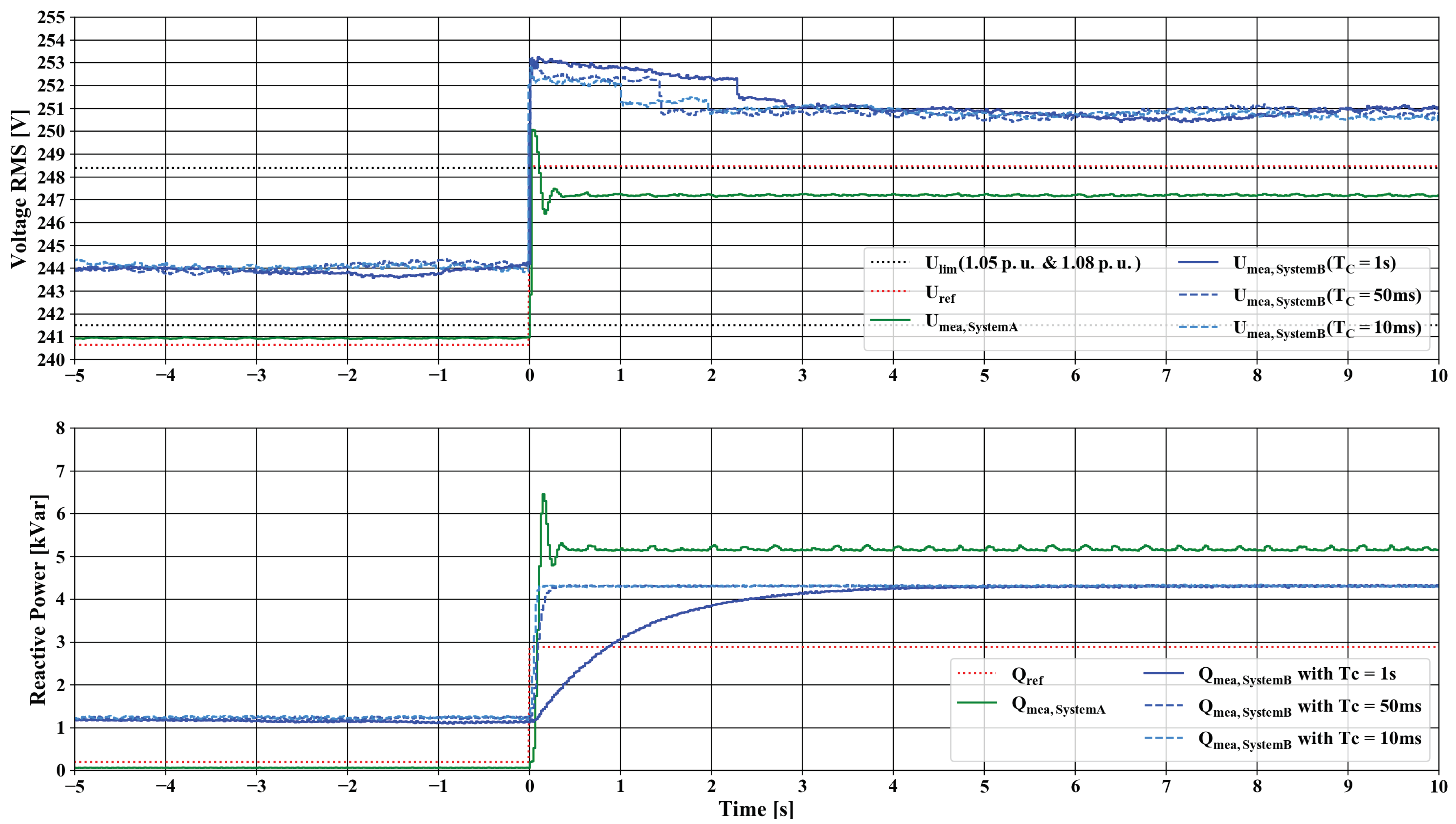
The evaluation depicted in Figure 10 focuses on the dynamic behaviour of the systems for the test scenario. This change of perspective can also be understood as change from the evaluation of the individual power interface to the evaluation of the complete PHIL setup. Statistical key parameters are listed in

Table 5. Statistical key parameter for the characterisation of system response for the step change of Phase A of the system.

Key Parameter	Time Frame	Dimension	System Setup A	System Setup B ${}^{†}$
ME(U)	PS	(V)	0.287	3.439
ME(U)	PT	(V)	−1.266	2.311
CC(U)	CT	(-)	0.991	0.994
DELTA(U)	PS	(V)	0.086	0.519
DELTA(U)	PT	(V)	0.153	0.660
STD(U)	PS	(V)	0.022	0.093
STD(U)	PT	(V)	0.029	0.138
$T_{Stabilisation}$	CT	(s)	0.620	3.732
MEAN(P) [STD(P)]	PS	(kW)	−1.613 [0.007]	−1.631 [0.023]
MEAN(P) [STD(P)]	PT	(kW)	−1.535 [0.012]	−1.547 [0.011]
MEAN(Q) [STD(Q)]	PS	(kvar)	+0.064 [0.003]	+1.238 [0.032]
MEAN(Q) [STD(Q)]	PT	(kvar)	+5.171 [0.033]	+4.310 [0.014]
$f_{Oscillation}$	CT	(Hz)	3.570	3.570

NA: not applicable; ${}^{†}$ $T_C$ = 10 ms is used; PS: pre-step; PT: post-stabilisation; CT: complete time frame.

to quantify the observations made in the figure. The one-period RMS values provided by the independent measurement device were used for this evaluation.

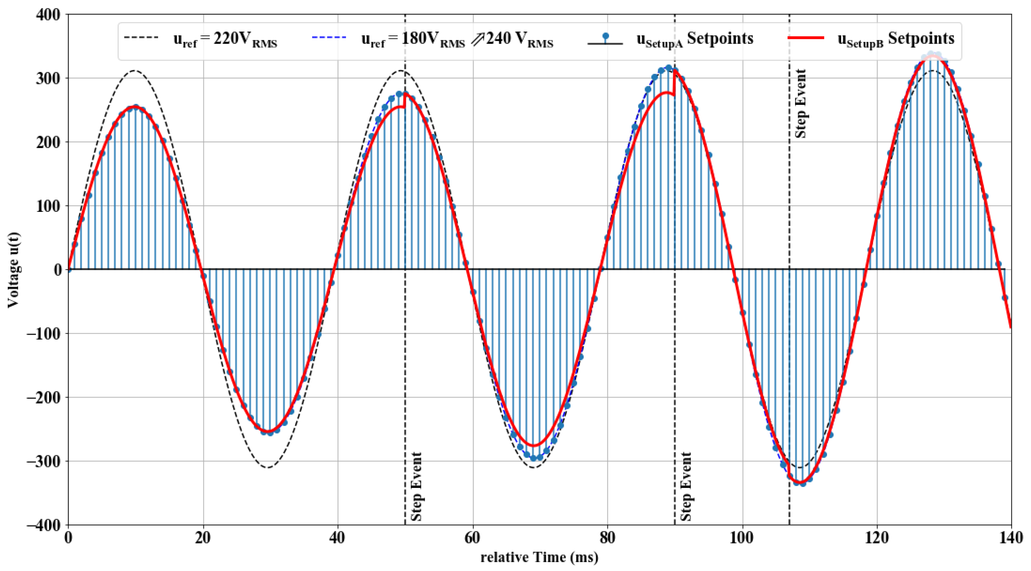
As a reference, the steady state values for the used grid model and implemented Q(U)-control are the parameters for the constructed curve which is plotted as a red dashed line. The experiments were carried out in individual runs. This means that the measured curves are aligned with the ideal step function. Therefore, an offset between the parameterised step and the actual step cannot be observed in the graphs. This offset was limited to a maximum of one simulation step. For System Setup B, this was limited to a maximum of 420 ms. Details regarding the simulation time are given in Section 5.5.

Three interesting aspects could be observed regarding the step functions: (i) the voltage deviation for the steady state situations before and after the step; (ii) the constancy of selected setpoints and the overall stabilisation time; and (iii) the stabilisation time, which is highly affected by the implemented control algorithm (e.g., Q(U) control) and the selected parameters.

The varying time constants of the Q(U) control could be observed when looking at the different responses of the PV inverter to the voltage step. For System Setups A and B, the inverter reacted immediately with a small time constant with a reactive power in-feed when the voltage changed. Smaller time constants resulted in faster reach of a steady state. For both setups, the reaction of the inverter was immediate when small time constants were used. In contrast to that was the calculated reaction to the changed reactive power in-feed by the system setups. For System Setup A, the reaction of the voltage happened immediately due to small time steps of the PHIL-setup, whereas, for System Setup B, the reaction was delayed in more discrete steps, which corresponded to the cycle time. As described in Section 4.3, the time constant suggested by the manufacturer is $T_C$ = 5 s, which will result in a highly damped system response. This seems to be a preferred strategy for DSO to prevent interference with multiple deployed systems.

Looking at the results of this test scenario, both systems showed a fairly linear offset to the reference value. This effect was reflected in the Mean Error (ME). However, the overall result was quite pleasurable showing a high Correlation Coefficient (CC) for both systems with a negligible difference between them. This occurrence could be expected as the calculated time for the time periods before and after the step function was included. The presented values were for Phase A to neutral of the three-phase system. Therefore, the readings were only a third of the in-feed of the three phase inverter. The oscillation already observed in Section 5.1 was quantified by the maximum spread (DELTA) and the resulting Standard Deviation (STD) of the voltage readings. As presented in the previous section, this related to the MPPT algorithm of the used PV inverters. As a result of the comparison of these values, one could see that System Setup A was more constant than System Setup B. The further examination also showed that these oscillations have a relatively constant subfundamental peak of around 3.570 Hz. This behaviour was also present for System Setup A but with a significantly lower amplitude. This also diminished when changing the voltage setpoint, and the oscillation was overlayed with other effects. Together with further analyses of the PI, it seemed that the immanent impedance of System Setup B was significantly higher than of System Setup A.

The upper dashed line represents the 1.08 p.u. value and, as one can see, the voltage of System Setup B never dropped below this parameterised limit of the Q(U) control. According to the given droop curve of the Q(U) controller, this resulted in a constant reactive power.

5.4. Comparison of the System Response for Voltage Ramp

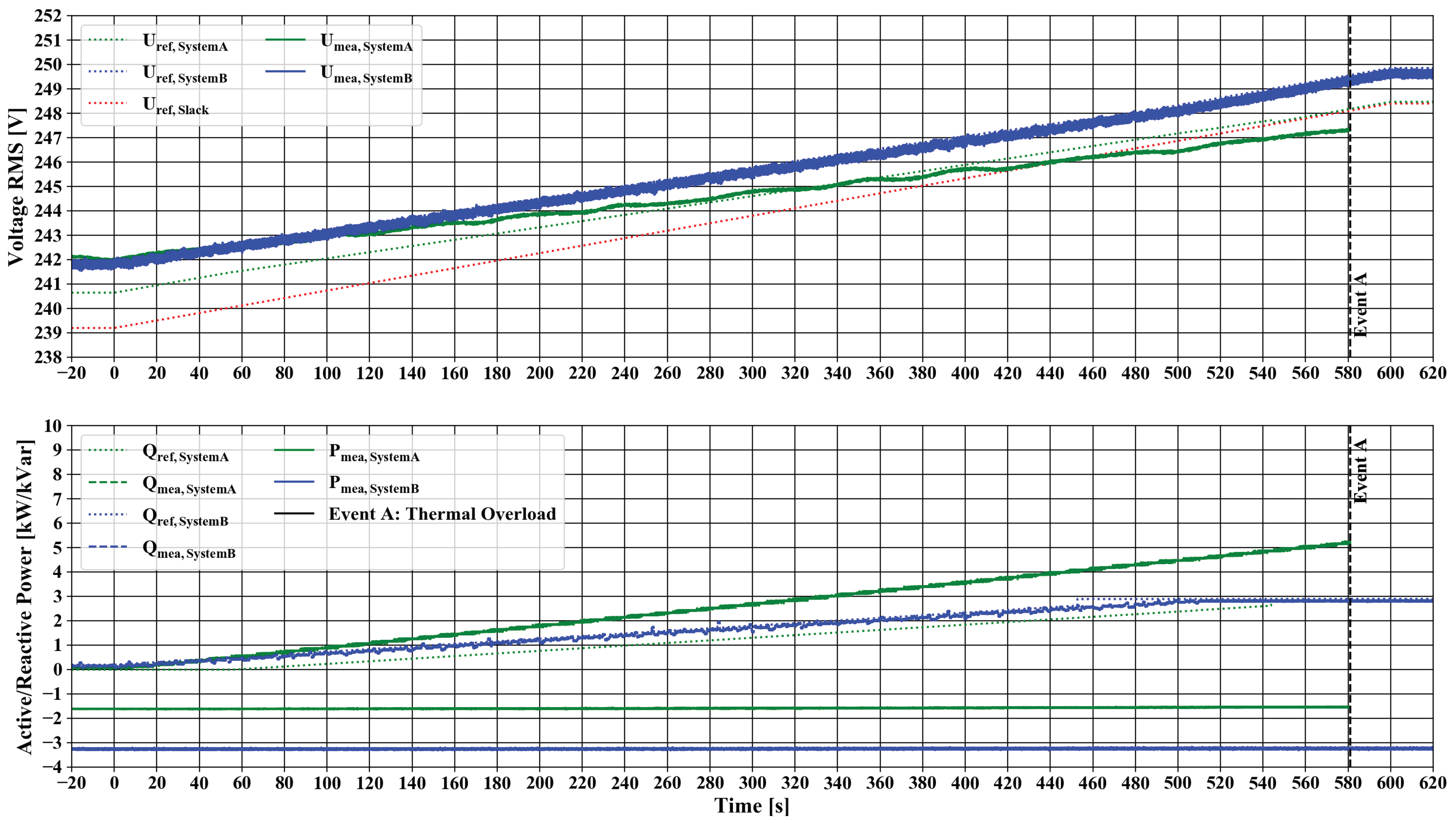
In comparison to the previous section where the focus lay on the comparison of the two systems in regard to the transient and dynamic behaviour when changing the voltage in an extreme manner, this section presents the comparison of both systems in the context of a slowly but constantly rising voltage level and the interaction of the Q(U) control. The results are shown in Figure 11. The corresponding statistical key figures are given in

Table 6. Statistical key parameter for the characterisation of system response for the ramp change. Comparison of ideal simulation and system output.

Key Parameter	Time Frame	Dimension	System Setup A	System Setup B
ME(U)	CT	(V)	0.210	−0.200
CC(U)	CT	(-)	0.999	0.999
DELTA(U)	CT	(V)	2.417	0.659
STD(U)	CT	(V)	0.660	0.113

CT: complete time frame.

(Statistical Key Figures for the Evaluation are shown in Appendix A). In contrast to the short term evaluation of the step function, this test scenario was executed with a variety of durations with up to 10 min of rise time. The scenario with a rise time of 10 min is outlined in the current section. To evaluate this rather long-term scenario, two different active power levels were chosen. This is due to the system properties of System Setup A, as the complete feed-in energy was dissipated by the PI. In the course of the experiment, issues regarding the overheating and thermal shutdown had to be tackled.

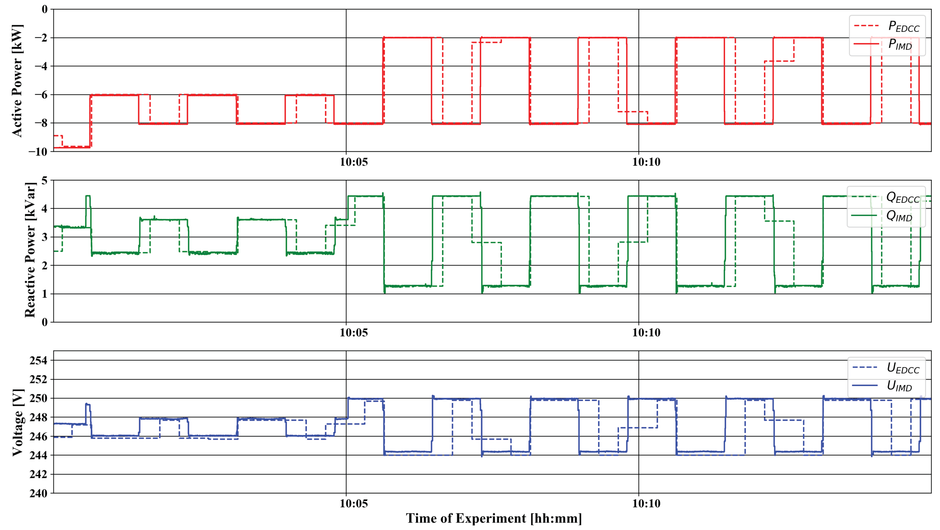
The reference curves for the ramp illustrate what is expected in theory. The red dashed line represents the constantly raising voltage level of the upstream grid with the inverter working against the voltage raise with feeding-in reactive power. When comparing the measured values, both systems showed a voltage deviation from the calculated value. For System Setup B, this deviation lay within the same order as it already could have been observed in the step experiment. With System Setup A, the voltage changed from over-voltage in respect to the reference curve to under-voltage due to a higher reactive power feed-in. The individual oscillation appeared in the same order of magnitude as in the previous scenario. The reactive power response of System Setup B became in the bigger time frame of this analysis quite pleasing. For System Setup A, the reactive in-feed was too high due to a different parameterisation.

The active in-feed power remained constant for both setups. The vertical line which is annotated with “Event A” represents the point where the power interface of System Setup A shuts down due to over-temperature.

5.5. Analysis of the Cycle Time for the Examined Setups

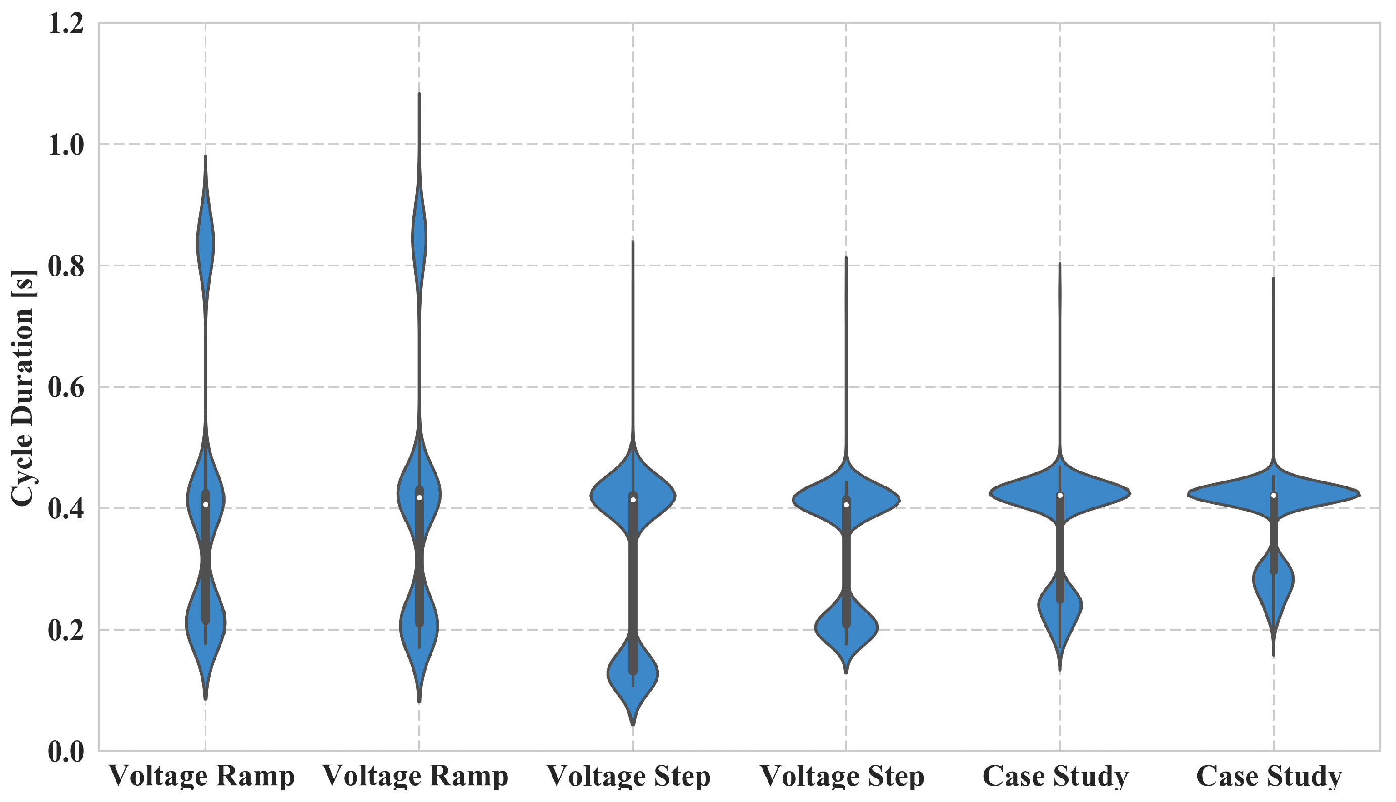
System Setup A was able to meet the time requirements due to its real-time control loop with a cycle time well below 50 $\mathsf{\mu }$s. For the QDPHIL system setup, the cycle time was significantly higher and required a more detailed analysis. As shown in Figure 12, the total cycle time remained under one second. The cycle time $t_{PHIL}$ for System Setup B consisted of the control loop in the main loop, the calculation of the new setpoints in PowerFactory, the control of the switched-mode amplifier Section 3.3 and the feedback of the measured values. The main control algorithm was implemented as a python script, which took about 20–30 ms runtime. Although the underlying interpreter required a bit more time to execute than a compiled program, new power interfaces can be quickly and flexibly integrated into the process using Python. This also applies to PowerFactory, which is controlled by a dedicated Python interface. Besides the python interface, there are several other ways to solve this task. Other possibilities such as OPC UA are discussed in detail in [54]. The solution was chosen because the whole functionality of PowerFactory’s internal scripting language (DPL) can also be addressed using the Python interface. Since Python has established itself as the standard in the given research infrastructure, it offers the possibility to use this interface also for the investigation of other research questions. Due to the simple grid model (see Section 4.2), the load flow calculation including feedback took 50 ms (±5), which can increase with larger modelled systems. The feedback contained the new set point for the switched mode amplifier. Its manufacturer provides a C# library, with which the new set point value can be communicated to the device via Ethernet. The time needed to execute the command could not be further optimised and lies at 250 ms (±50). One possibility to actually achieve faster response times is to use the option of analog control of the network simulator in “amplifier mode”. To access the C# interface, a helper application was used, which is coupled to the python main loop via a named pipe. Subsequently, a new actual value was queried by Modbus/TCP from the measuring device and thus the control loop started again. This last step required 100 ms (±20). Overall, a $t_{PHIL}$ with a median of 420 ms could be achieved with System Setup B. The cycle time shown for different experiments is depicted as violin plot in Figure 12. The density representation shows two and three clusters for the cycle time with the highest density around the median. The second cluster is in range of 0.2–0.3 s. Due to the added IEC61850 simulator function used in the case study, this cluster is moved towards the median.

6. Phase 2: Test of A Complex Smart Grid Control Regime

In the following section, the experiment is introduced briefly which complies with the requirements given in Section 3.1. This experiment was the main example use case when designing the comparison of the previous section. Therefore, this section describes the actual process of setting up and carrying out this experiment. The scope of the contribution is therefore widened and enriched with real results. Moreover, finding a flawless control algorithm was not the aim of the carried out experiment. The chosen algorithm is not suitable for this application but shows the necessity of the complete testing procedure. Preliminary results are presented in [55] and are extended within this section.

6.1. Description of the Case Study Experiment

6.1.1. System under Test

The purpose of this case study experiment was to observe the performance and reaction of the EUT responding to smart grid control strategies in a controlled environment. In this case, the EUT was a Fronius PV inverter with its active power feed-in regulated by a coordinated voltage control strategy. The inverter has a nominal active power of 20 kW; however, due to active power restriction, the nominal value was limited to 10 kW during the experiment. The Q(U) setting applied to the EUT was the same as in the previous Phase 1. To distinguish the EUT from the SUT, the SGAM Layer representation in Figure 13 can be used. The SUT can be identified as the complete construction shown in the diagram which consists of a Supervisory Control and Data Acquisition (SCADA) system, a fleet management for the smartRTUs (also referred to as Controllable Local Systems (CLS) Management), traditional RTUs and smartRTUs and the depicted primary equipments.

6.1.2. Communication and Control Infrastructure

The control infrastructure consists of a grid control system, a Remote Terminal Unit (RTU) that acts as a protocol gateway, a fleet management system for the RTU and the controlled PV inverter. As grid control system, the experimental Distribution Control Center (EDCC) at Ulm University of applied Science is used. The operational measurements from the PV inverter are gathered by the RTU via the SunSpec protocol [57] and transmitted to the control system via the IEC 61850-7-4 [58] and IEC 61850-7-420 [59] standard. This concept complies with German regulations regarding the use of the SmartMeter infrastructure. Further information is given in [55,60].

6.1.3. Control Function

The virtual Intelligent Electronic Device (IED) Server transmits the grid information via Virtual Private Network (VPN) to the EDCC, where a voltage control algorithm was implemented and configured as a visual basic script. As a result of interacted hardware measurement and software simulation, a power curtailment setpoint, represented as a percentage value with respect to nominal active power, was sent back to the RTU and was subsequently forwarded to the PV inverter. The voltage regulation would be triggered when the voltage was bigger than 1.05 p.u. The active power curtailment was transmitted to the inverter in gradual steps by 10% an exceeded 0.005 p.u. The used control algorithm can be described by the following equation:

$$P_{Limit}=P_{nominal}\ast f_{curtailment}\left(U_{PCC}\right)\left\{\begin{array}{cc}f=0.0\hfill & U_{PCC}\ge 1.080\mathrm{p}.\mathrm{u}.\hfill \\ f=0.1\hfill & U_{PCC}\ge 1.075\mathrm{p}.\mathrm{u}.\hfill \\ & ⋮\hfill \\ f=0.9\hfill & U_{PCC}\ge 1.055\mathrm{p}.\mathrm{u}.\hfill \\ f=1.0\hfill & U_{PCC}\le 1.050\mathrm{p}.\mathrm{u}.\hfill \end{array}\right.$$

(9)

It might appear that the algorithm is not suitable for the task assigned as it would lead to an oscillation behaviour. Nonetheless, the algorithm was chosen fully aware of this circumstance. A clearly defined oscillation is easily observable and the effect is hard to be superimposed by other effects.

6.2. Results of the Case Study Experiment

The described methodology was used to test and evaluate the setup described in the previous section. The simulated OLTC of the grid was actuated to step through the voltage range and to trigger the two (Q(U) and P(U)) control regimes. Figure 14 shows the results of the executed experiment as a plot of active andreactive power over the voltage at the PCC of the inverter. The described steps can be seen in clusters of data points in the diagram. The characteristics for the local Q(U) and the superior P(U) control are represented as lines as well. The green coloured area represents the anticipated deviation for the Q(U) control due to output filters and error of the measurements from the inverter as well as from the independent measurement. Nevertheless, the measured values for Q(U) control remained close to the desired characteristics. Looking at the P(U) control governed by the SCADA system, it can be noticed that the deactivated P(U) control resulted in stable operating points at different set points of the simulated voltage regulator of the transformer. The in-feed power of the inverter was not curtailed. With activated P(U) control, the purple coloured area represents the undesired voltage range. As the control-algorithm is a very basic lookup-table, the voltage has to be within this area for at least one transmitted period.

In the active power and voltage plot in Figure 14, a few control actions of the control algorithm are depicted. The value pairs form four main clusters, which are inherent to the used setup. The direct causes of the change from one cluster to another are described in the following list:

• (A → B) The voltage is within the undesired range. In addition, curtailment command is transmitted after the executed cycle of the control algorithm. There is a decrease in feed-in power due to the curtailment command, and slightly reduced voltage level due to the inherent properties of the voltage source (please refer to the previous section).
• (B → C) Due to a new voltage set point for voltage source, the voltage readings decrease after a load flow calculation is carried out.
• (C → D) With the next performance of the tested control algorithm, the voltage is in an acceptable range, and the curtailment is retracted. Due to the inherent properties of the voltage source, the voltage increases slightly.
• (D → A) With the next carried out load flow calculation, the system state returns to A.

The analysis showed that the proposed setup with a simple test algorithm is working. This is visualised in the time-series plot of Figure 15, where the measurements of the independent measurement device and the transmitted readings of the SCADA system are compared. Due to the automatically sent commands of the SCADA system, the field gateway passed the curtailment to the inverter. The inverter limited the feed-in to the desired value. This led to a change in voltage level due to the PHIL setup. As result of the experiment, the postulated oscillation occurred; nonetheless, the control algorithm would not be suitable for a real grid operation. When comparing the measurement and the transmitted values of the SCADA system, the discretisation evoked by the technical constraints was clearly observable.

7. Discussion of the Results

The experiments of Phase 1 showed that the System Setups A and B have been able to provide three-phase voltage systems, which are suitable to synchronise the given PV inverters, and started to operate properly. The modelled grid was used for a load flow calculation, and the extracted voltage signal was forwarded to the power interface. The Q(U)-function of the inverter was also tested. The biggest draw back observed in the carried out experiments was the significant voltage deviation for System Setup B which ranged from 2.3 to 3.4 $V_{RMS}$ for the step function experiment. Based on further examinations, we assume that the offset was caused by an immanent impedance. In these examinations, a proportional offset from the idle state voltage setpoint to the idle state voltage present at the terminals of the power interface occurred. When changing the consumed or feeding power independent of voltage set point, the voltage offset changed as well. Therefore, it is expected that the offset could be compensated with simple correction equations, which do not even introduce another controller to the system. Alternatively, the PI of System Setup B could be replaced with the superior PI of System Setup A, which featured a lower impedance and would therefore have reduced the undesired effects. Nonetheless, the dynamic properties would stay the same. Both experiments showed the correlation coefficient is >0.99 for both of the system setups. Since all of experiments presented in this contribution have in common that they utilised voltage setpoints, and a current or power, as feedback loops, the results presumably are not applicable for current type experiments. Regarding the cycle time of the given QDPHIL setup, a median of 0.42 s could be achieved. The communication between the simulation and the PI has a big share of approximately 250 ms of this process and offers the possibility for further improvements.

The occurred automatic power shut-off to prevent overheating of the PI of System Setup A could be tackled by using an additional load to prevent the feed-in energy being dissipated within the PI. This would also alter the Thevenin-equivalent of the setup, which might be undesirable. Regarding the quality of the provided voltage signals, both systems generated negligible amounts of harmonics. To represent real grid situations, introducing a realistic amount of harmonics must be considered.

Regarding the soft facts, involving setup and training, System Setup B seemed less challenging as the options were more limited. In addition, the software PowerFactory is one of the standard tools used at Ulm University of Applied Science not only for real-time simulation but also for scenario and time series analysis of distribution grids. Using those models and calculation algorithms in pure simulation experiments and in PHIL testing is beneficial. The models had to be setup up only once and results from the simulation were helpful in the PHIL experiment design. In addition, the results from the PHIL experiment could improve the models implemented in the simulation environment.

Another difference between the PI of the two setups was the maximal frequency at which the systems could reproduce harmonics. For System Setup A, this was limited to 30 kHz, whereas, for System Setup B, this was limited to 5 kHz. This aspect was not a prominent requirement for the contemplated usage, however. The described aspects are given in a short overview in

Table 7. Findings of experiments of Phase 0 and Phase 1.

	System Setup A	System Setup B
Pros (+)	small cycle time (≤$50\mathsf{\mu }\mathrm{s}$) multiple calculation methods (phasor simulation, transient simulation) low immanent impedance	regenerates energy during the test
Neutral (#)	specific usage of the simulation tool	sufficient cycle time (≤1 s) variation in cycle time only voltage type experiments
Cons (-)	over heating occurs dissipates energy during test run	one calculation method (steady state) high immanent impedance

.

8. Conclusions and Outlook

The conclusions of this work are manifold and can be divided into the following parts. The first part summarises the findings of the voltage step and ramp experiments carried out in Phase 1, while the second part discusses the findings of the case study (Phase 2). In the third part, the conclusions are provided and finally the planned improvements and the utilisation of the entire setup is summed up.

The contribution presents results for a comparison of two PHIL setups—these were called System Setup A for the combination of an Opal-RT system and Spitzenberger Spies PAS PI and System Setup B for the combination of a Digsilent PowerFactory instance and a Regatron TC.ACS PI. The use case—testing of coordinated smart grid control function in an undisturbed operation—which was examined with both setups is only a subset of the capabilities of classical PHIL setups. The expected outcome of the experiments was that both systems are capable of solving this task. The fundamental difference between both systems were the calculation principles which are phasor calculation for System Setup A and the use of steady-state simulation for System Setup B. For this comparison, two scenarios were considered: (i) change of voltage level with a step; and (ii) a ramp function in the modelled grid at slack element. As a result, different levels of accuracy and continuity of the output signal were observed. The difference of the systems are apparent for the reaction of the Q(U) controller of the PV inverter within the test environment. If the time constant of the Q(U) controller is significantly lower than the cycle time, System Setup B shows discrete steps of the voltage and the stabilisation time is prolonged. As an overall statement, System Setup B is suitable for the use case described in Section 3.1. One issue which occurred during the test was an offset between the set-point sent to the PI and the actual voltage measured at the terminals. It is suspected that this problem is caused by the high immanent impedance of System Setup B. This problem needs to be tackled.

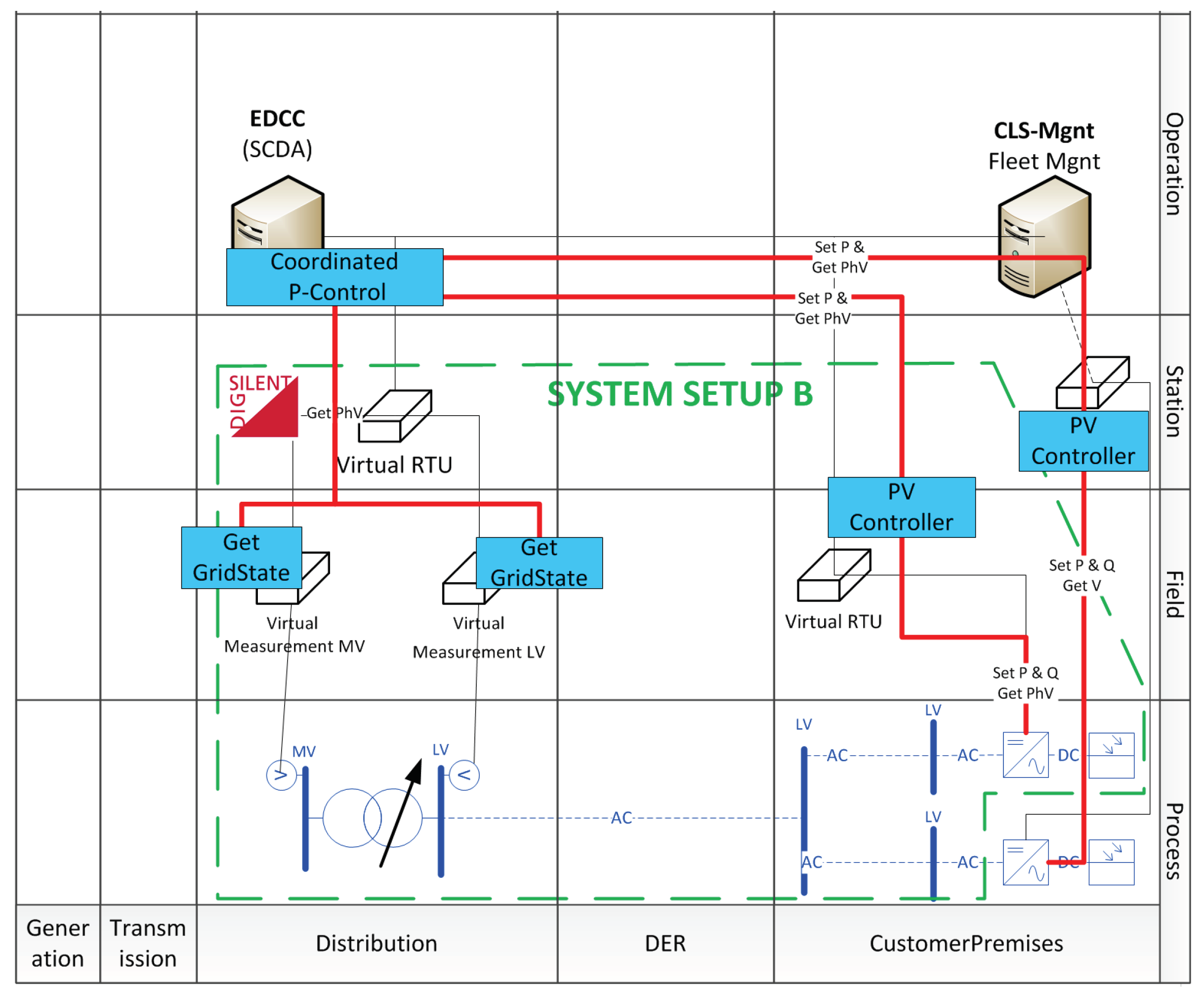
In the second part of this contribution, an actual utilisation of System Setup B is presented, which shows the intended use for a combined PHIL and SIL testing of complex smart grid control functions. The use of the SGAM presentation provided a basis for a common understanding of the presented test. This is in line with the holistic testing description introduced by the ERIgrid Consortium [61]. Due to the description of the planned scenario, the different facilities were able to implement sub-functions in an efficient manner and were able to test the relevant sub-functions before the actual experiment. As the outcome of this case study, the tested central control algorithm is not useful for actual grid operation, as it was anticipated and deliberately chosen at the stage of test design. However, the gathered data provided a good basis for the validation of the process. In addition, the carried out experiment is a successful pilot test for the application of the RTU. It showed clearly that gathering of relevant measured values at the grid connection point and the generation unit is possible with the implemented SunSpec to the IEC 61850 converter. The other way round was tested as well and the curtailment of the PV inverter was successfully carried out.

As a conclusion, it can be stated that there was a significant difference in the working principle of the two system setups. Both systems could provide a function essential for the evaluation of EUT and SUT with respect to the requirements stated in Section 3.1. The PHIL System Setup A was more accurate and showed more capabilities than the QDPHIL System Setup B but this came at the price of a more complex system regarding modelling, setup and operation than it was required in System Setup B. In addition, the expenditures for purchase and maintenance have been higher for System Setup A compared to System Setup B. Regarding the use of electric energy, the PI of System Setup B was able to feed back into the grid, whereas the linear PI of System Setup A dissipated the energy.

As further steps, System Setup B will be improved to solve the issues regarding the occurring offset without the use of an additional controller. As first evaluations suggest the effects are fairly linear and are likely caused by a high immanent impedance of the PI, further analyses and engineering will be necessary. These will also include considerations regarding the implementation of the immanent impedance in the grid model. The implemented System Setup B is and will be used at the Ulm University of Applied Science in the course of different research projects. The setup will be mainly used for pilot testing of applications involving small decentralised control units in combination with the German Smart Meter Infrastructure, which consists of the combination of Smart Meter, Smart Meter Gateway and CLS-Module to enable information gathering and control of small generation units such as PV inverters, as tested in the case study of Section 6. These measurements are necessary in preparation of a broader deployment in the demonstration project C/sells [62]. As specific suggestions for future work, the examination of effect of different interface algorithms and a detailed study of the influence communication interface between simulation and power interface for the quasi-static PHIL setups can be given. In this context, the implementation of the IA transmission line model is considered. This would enable the utilisation of a available and standardised line impedance network which is typically used for tests according to IEC 61000 series standard.

References

1. Di Silvestre, M.L.; Favuzza, S.; Riva Sanseverino, E.; Zizzo, G. How Decarbonization, Digitalization and Decentralization are changing key power infrastructures. Renew. Sustain. Energy Rev. 2018, 93, 483–498. [Google Scholar] [CrossRef]
2. Field, C.B. Climate Change 2014: Impacts, Adaptation, and Vulnerability: Working Group II Contribution to the Fifth Assessment Report of the Intergovernmental Panel on Climate Change; Cambridge University Press: Cambridge, UK, 2014. [Google Scholar]
3. Stocker, T. Climate Change 2013: The Physical Science Basis: Working Group I Contribution to the Fifth Assessment Report of the Intergovernmental Panel on Climate Change; Cambridge University Press: Cambridge, UK, 2014. [Google Scholar]
4. United Nations. Paris Agreement; United Nations: New York, NY, USA, 2015. [Google Scholar]
5. Farhangi, H. The path of the smart grid. IEEE Power Energy Mag. 2010, 8, 18–28. [Google Scholar] [CrossRef]
6. Liserre, M.; Sauter, T.; Hung, J. Future Energy Systems: Integrating Renewable Energy Sources into the Smart Power Grid Through Industrial Electronics. IEEE Ind. Electron. Mag. 2010, 4, 18–37. [Google Scholar] [CrossRef]
7. Gungor, V.C.; Sahin, D.; Kocak, T.; Ergut, S.; Buccella, C.; Cecati, C.; Hancke, G.P. Smart Grid Technologies: Communication Technologies and Standards. IEEE Trans. Ind. Inform. 2011, 7, 529–539. [Google Scholar] [CrossRef] [Green Version]
8. Benz, T. The Cellular Approach: The Basis of Successful, Cross-Regional Energy Transition; VDE-Study; VDE Verband der Elektrotechnik, Elektronik, Informationstechnik e. V: Frankfurt, Germany, 2015. [Google Scholar]
9. Martini, L.; Brunner, H.; Rodriguez, E.; Caerts, C.; Strasser, T.I.; Burt, G.M. Grid of the future and the need for a decentralised control architecture: The web-of-cells concept. CIRED-Open Access Proc. J. 2017, 2017, 1162–1166. [Google Scholar] [CrossRef]
10. Kariniotakis, G.; Martini, L.; Caerts, C.; Brunner, H.; Retiere, N. Challenges, innovative architectures and control strategies for future networks: The Web-of-Cells, fractal grids and other concepts. CIRED-Open Access Proc. J. 2017, 2017, 2149–2152. [Google Scholar] [CrossRef]
11. Lund, P. The Danish Cell Project—Part 1: Background and General Approach. In Proceedings of the 2007 IEEE Power Engineering Society General Meeting, Tampa, FL, USA, 24–28 June 2007; pp. 1–6. [Google Scholar]
12. Bitkom Bundesverband Informationswirtschaft, Telekommunikation und neue Medien e.V. Ausfallsicherheit des Energieversorgungssystems—Von der Robustheit zur Resilienz; Bitkom: Berlin, Germany, 2018. [Google Scholar]
13. Scharte, B.; Thoma, K. Resilienz—Ingenieurwissenschaftliche Perspektive. In Multidisziplinäre Perspektiven der Resilienzforschung; Wink, R., Ed.; Springer Fachmedien Wiesbaden: Wiesbaden, Germany, 2016; pp. 123–150. [Google Scholar]
14. Ebe, F.; Idlbi, B.; Stakic, D.; Heilscher, G.; Birkelbach, J.; Gutekunst, F.; Enzenhöfer, R. Abstimmungskaskade als Werkzeug für eine zellbasierte Infrastruktur—Allgemeingültiger Prozess für die Koordinierung von Netzzellen. In Proceedings of the Tagungsunterlagen zukünftige Stromnetze für erneuerbare Energien, Berlin, Germany, 30–31 January 2018. [Google Scholar]
15. Wang, H.; Kraiczy, M.; Schmidt, S.; Wirtz, F.; Toebermann, J.C.; Ernst, B.; Kaempf, E.; Braun, M. Reactive Power Management at the Network Interface of EHV- and HV Level: Assessment of Technical and Economic Potential Based on a Case Study for Bayernwerk Netz GmbH. In Proceedings of the International ETG Congress 2017, Bonn, Germany, 28–29 November 2017. [Google Scholar]
16. Vogt, M.; Marten, F.; Lower, L.; Horst, D.; Brauns, K.; Fetzer, D.; Menke, J.H.; Troncia, M.; Hegemann, J.; Tobermann, C.; Braun, M. Evaluation of interactions between multiple grid operators based on sparse grid knowledge in context of a smart grid co-simulation environment. In Proceedings of the 2015 IEEE Eindhoven PowerTech, Eindhoven, The Netherlands, 29 June–2 July 2015; pp. 1–6. [Google Scholar]
17. Drayer, E.; Hegemann, J.; Gehler, S.; Braun, M. Resilient distribution grids—Cyber threat scenarios and test environment. In Proceedings of the 2016 IEEE PES Innovative Smart Grid Technologies Conference Europe (ISGT-Europe), Ljubljana, Slovenia, 9–12 October 2016; pp. 1–6. [Google Scholar]
18. Dena-Verteilnetzstudie: Ausbau- und Innovationsbedarf der Strom Veteilnetze in Deutschland bis 2030; DeNA: Berlin, Germany, 2018.
19. Strasser, T.; Pröstl Andrén, F.; Lauss, G.; Bründlinger, R.; Brunner, H.; Moyo, C.; Seitl, C.; Rohjans, S.; Lehnhoff, S.; Palensky, P.; et al. Towards holistic power distribution system validation and testing—An overview and discussion of different possibilities. e & i Elektrotechnik und Informationstechnik 2017, 134, 71–77. [Google Scholar]
20. De Jong, E.; Graaff, R.; Vaessen, P.; Crolla, P.; Roscoe, A.; Lehfuss, F.; Lauss, G.; Kotsampopoulos, P.; Gafaro, F. European White Book on Real-Time Power Hardware-in-the-Loop Testing; DERlab e.V.: Kassel, Germany, 2012. [Google Scholar]
21. Omar Faruque, M.D.; Strasser, T.; Lauss, G.; Jalili-Marandi, V.; Forsyth, P.; Dufour, C.; Dinavahi, V.; Monti, A.; Kotsampopoulos, P.; Martinez, J.A.; et al. Real-Time Simulation Technologies for Power Systems Design, Testing, and Analysis. IEEE Power Energy Technol. Syst. J. 2015, 2, 63–73. [Google Scholar] [CrossRef]
22. Guillaud, X.; Faruque, M.O.; Teninge, A.; Hariri, A.H.; Vanfretti, L.; Paolone, M.; Dinavahi, V.; Mitra, P.; Lauss, G.; Dufour, C.; et al. Applications of Real-Time Simulation Technologies in Power and Energy Systems. IEEE Power Energy Technol. Syst. J. 2015, 2, 103–115. [Google Scholar] [CrossRef] [Green Version]
23. Lauss, G.; Faruque, M.O.; Schoder, K.; Dufour, C.; Viehweider, A.; Langston, J. Characteristics and Design of Power Hardware-in-the-Loop Simulations for Electrical Power Systems. IEEE Trans. Ind. Electron. 2016, 63, 406–417. [Google Scholar] [CrossRef]
24. Roscoe, A.J.; Mackay, A.; Burt, G.M.; McDonald, J.R. Architecture of a Network-in-the-Loop Environment for Characterizing AC Power-System Behavior. IEEE Trans. Ind. Electron. 2010, 57, 1245–1253. [Google Scholar] [CrossRef] [Green Version]
25. Lehfuss, F.; Lauss, G.; Kotsampopoulos, P.; Hatziargyriou, N.; Crolla, P.; Roscoe, A. Comparison of multiple power amplification types for power Hardware-in-the-Loop applications. In Proceedings of the 2012 IEEE Complexity in Engineering (COMPENG), Aachen, Germany, 11–13 June 2012; pp. 1–6. [Google Scholar]
26. Brandl, R. Operational Range of Several Interface Algorithms for Different Power Hardware-In-The-Loop Setups. Energies 2017, 10, 1946. [Google Scholar] [CrossRef]
27. Ren, W.; Steurer, M.; Baldwin, T.L. Improve the Stability and the Accuracy of Power Hardware-in-the-Loop Simulation by Selecting Appropriate Interface Algorithms. IEEE Trans. Ind. Appl. 2008, 44, 1286–1294. [Google Scholar] [CrossRef]
28. Ou, T.C.; Lu, K.H.; Huang, C.J. Improvement of Transient Stability in a Hybrid Power Multi-System Using a Designed NIDC (Novel Intelligent Damping Controller). Energies 2017, 10, 488. [Google Scholar] [CrossRef]
29. Helmedag, A.; Isermann, T.; Monti, A. Fault ride through certification of wind turbines based on a power hardware in the loop setup. In Proceedings of the 2013 IEEE International Workshop on Applied Measurements for Power Systems (AMPS), Aachen, Germany, 25–27 September 2013; pp. 150–155. [Google Scholar]
30. Kleftakis, V.; Rigas, A.; Vassilakis, A.; Kotsampopoulos, P.; Hatziargyriou, N. Power-Hardware-in-the-loop simulation of a D-STATCOM equipped MV network interfaced to an actual PV inverter. In Proceedings of the IEEE PES ISGT Europe 2013, Copenhagen, Denmark, 6–9 October 2013; pp. 1–5. [Google Scholar]
31. Brandl, R. Improved Methods for Real-time Simulation and Hardware-in-the-loop. In Proceedings of the International Conference on Integration of Renewable and Distributed Energy Resources (IRED), Vienna, Austria, 16–19 October 2018. [Google Scholar]
32. Strasser, T.I.; Moyo, C.; Bründlinger, R.; Lehnhoff, S.; Blank, M.; Palensky, P.; van der Meer, A.A.; Heussen, K.; Gehrke, O.; Rodriguez, J.E.; et al. An Integrated Research Infrastructure for Validating Cyber-Physical Energy Systems. In Industrial Applications of Holonic and Multi-Agent Systems; Mařík, V., Wahlster, W., Strasser, T., Kadera, P., Eds.; Springer International Publishing: Cham, Switzerland, 2017; pp. 157–170. [Google Scholar]
33. CEN-CENELEC-ETSI Smart Grid Coordination Group. Smart Grid Reference Architecture; CEN-CENELEC-ETSI Smart Grid Coordination Group: Brussels, Belgium, 2012. [Google Scholar]
34. Maniatopoulos, M.; Lagos, D.; Kotsampopoulos, P.; Hatziargyriou, N. Combined control and power hardware in-the-loop simulation for testing smart grid control algorithms. IET Gener. Trans. Distrib. 2017, 11, 3009–3018. [Google Scholar] [CrossRef]
35. Kundur, P.S.; Balu, N.J. (Eds.) Power System Stability and Control; The EPRI Power System Engineering Series; McGraw-Hill: New York, NY, USA, 1994. [Google Scholar]
36. Mahseredjian, J.; Dinavahi, V.; Martinez, J.A. Simulation Tools for Electromagnetic Transients in Power Systems: Overview and Challenges. IEEE Trans. Power Deliv. 2009, 24, 1657–1669. [Google Scholar] [CrossRef]
37. Andrén, F.; Lehfuss, F.; Jonke, P.; Strasser, T.; Rikos, E.; Kotsampopoulos, P.; Moutis, P.; Belloni, F.; Sandroni, C.; Tornelli, C.; et al. DERri Common Reference Model for Distributed Energy Resources—Modeling scheme, reference implementations and validation of results. e & i Elektrotechnik und Informationstechnik 2014, 131, 378–385. [Google Scholar]
38. Martinez, J.A.; Mahseredjian, J. Load flow calculations in distribution systems with distributed resources. A review. In Proceedings of the 2011 IEEE Power and Energy Society General Meeting, Detroit, MI, USA, 24–29 July 2011; pp. 1–8. [Google Scholar]
39. Lundstrom, B.; Chakraborty, S.; Lauss, G.; Brundlinger, R.; Conklin, R. Evaluation of system-integrated smart grid devices using software- and hardware-in-the-loop. In Proceedings of the 2016 IEEE Power & Energy Society Innovative Smart Grid Technologies Conference (ISGT), Minneapolis, MN, USA, 6–9 September 2016; pp. 1–5. [Google Scholar]
40. Holt, C.; Kong, A.; St. Leger, A.; Bennett, D. Communications network emulation for smart grid test-bed. In Proceedings of the 2016 IEEE Power and Energy Society General Meeting (PESGM), Boston, MA, USA, 17–21 July 2016; pp. 1–5. [Google Scholar]
41. Babazadeh, D.; Chenine, M.; Zhu, K.; Nordstrom, L.; Al-Hammouri, A. A platform for wide area monitoring and control system ICT analysis and development. In Proceedings of the 2013 IEEE PowerTech Grenoble Conference, Grenoble, France, 16–20 June 2013; pp. 1–7. [Google Scholar]
42. Spitzenberger & Spies GmbH & Co. KG, Data Sheet: PAS Series of 4-Quadrant Amplifiers. Available online: https://www.spitzenberger.de/weblink/1002 (accessed on 24 August 2018).
43. Opal-RT Technologies Inc. Product Sheet:Real-Time Simulation Solutions for Power Grids and Power Electronics. Available online: https://www.opal-rt.com/wp-content/themes/enfold-opal/pdf/L00161_0260.pdf (accessed on 24 August 2018).
44. Fronius International GmbH, Data Sheet: FRONIUS Symo Series. Available online: http://www.fronius.com/~/downloads/Solar%20Energy/Datasheets/SE_DS_Fronius_Symo_DE.pdf (accessed on 24 August 2018).
45. Dewetron GmbH, Data Sheet: DEWE -800. Available online: https://www.dewetron.com/wp-content/uploads/2016/05/dewetron_dewe-800_e-1.pdf (accessed on 24 August 2018).
46. DIgSILENT GmbH, Data Sheet: PowerFactory 2018. Available online: https://www.digsilent.de/en/downloads.html (accessed on 24 August 2018).
47. Regatron AG, Data Sheet: TC.ACS Programmable AC Source-Sink Series. Available online: https://www.regatron.com/service/download/brochures/tc.acs-series-brochure.pdf (accessed on 24 August 2018).
48. Janitza Electronics GmbH, Data Sheet: Universal Measuring Device UMG 96—Operating Instructions. Available online: https://www.janitza.de/betriebsanleitungen.html?file=files/download/manuals/current/UMG96/Janitza-Manual-UMG96-all-versions-en.pdf (accessed on 24 August 2018).
49. Network Technology/Network Operation Forum at VDE (VDE|FNN). VDE-AR-N 4105:2011-08 Power Generation Systems Connected to the Low-Voltage Distribution Network; VDE-VERLAG GMBH: Berlin, Germany, 2010. [Google Scholar]
50. Elbs, C.; Pardatscher, R. Einsatz der Q(U)-Regelung bei der Vorarlberger Energienetze GmbH; Vorarlberger Energienetze: Bregenz, Austria, 2014. [Google Scholar]
51. Energie-Control Austria. TOR D4: Parallelbetrieb von Erzeugungsanlagen mit Verteilernetzen; Energie-Control: Vienna, Austria, 2016.
52. International Electrotechnical Commission. IEC 61000-3-3:2013 Electromagnetic Compatibility (EMC)—Part 3-3: Limits-Limitation of Voltage Changes, Voltage Fluctuations and Flicker in Public Low-Voltage Supply Systems, for Equipment with Rated Current < 16 A Per Phase and Not Subject to Conditional Connection; International Electrotechnical Commission: Geneva, Switzerland, 2013. [Google Scholar]
53. KACO New Energy GmbH, Data Sheet: Powador 12-20 TL3. Available online: http://kaco-newenergy.com/fileadmin/data/downloads/products/Powador_12.0-20.0_TL3/Data%20Sheets/DTS_PW_12-20_TL3_en.pdf (accessed on 24 August 2018).
54. Stifter, M.; Andren, F.; Schwalbe, R.; Tremmel, W. Interfacing PowerFactory: Co-simulation, Real-Time Simulation and Controller Hardware-in-the-Loop Applications. In PowerFactory Applications for Power System Analysis; Power Systems; Gonzalez-Longatt, F.M., Rueda, J.L., Eds.; Springer: Cham, Switzerland, 2014; pp. 343–366. [Google Scholar]
55. Ebe, F.; Idlbi, B.; Casel, M.; Kondzialka, C.; Chen, S.; Morris, J.; Heilscher, G.; Seitl, C.; Bründlinger, R.; Strasser, T. An approach for validating and testing micro grid and cell-based control concepts. In Proceedings of the CIRED Workshop 2018, Ljubljana, Slovenia, 7–8 June 2018. [Google Scholar]
56. Santodomingo, R.; Uslar, M.; Gottschlak, M.; Goering, A.; Nordstrom, L.; Valdenmaiier, G. The discern tool support for knowledge sharing in large smart grid projects. In Proceedings of the CIRED Workshop 2016, Helsinki, Finland, 14–15 June 2016. [Google Scholar]
57. SunSpec Alliance. SunSpec Technology Overview; SunSpec Alliance: San Jose, CA, USA, 2015. [Google Scholar]
58. International Electrotechnical Commission. IEC 61850 Part 7-4: Basic Communication Structure—Compatible Logical Node Classes and Data Object Classes; International Electrotechnical Commission: Geneva, Switzerland, 2010. [Google Scholar]
59. International Electrotechnical Commission. IEC 61850 Part 7-420: Basic Communication Structure—Distributed Energy Resources Logical Nodes; International Electrotechnical Commission: Geneva, Switzerland, 2009. [Google Scholar]
60. Heilscher, G.; Chen, S.; Lorenz, H.; Ebe, F.; Kondzialka, C.; Kaufman, T.; Hess, S.; Wening, J. Secure Energy Information Network in Germany—Demonstration of Solar-, Storage- and E-Mobility Applications. In Proceedings of the 8th International Workshop on Integration of Solar Power into Power Systems, Stockholm, Sweden, 16–17 October 2018. [Google Scholar]
61. Heussen, K.; Morales Bondy, D.E.; Nguyen, V.H.; Blank, M.; Klingenberg, T.; Kulmala, A.; Abdulhadi, I.; Pala, D.; Rossi, M.; Carlini, C.; et al. D-NA5.1 Smart Grid Configuration Validation Scenario Description Method; ERIGrid: Vienna, Austria, 2017. [Google Scholar]
62. Smart Grids-Plattform Baden-Württemberg e.V. C/Sells-Guiding principle. Available online: https://www.csells.net/en/about-c-sells/guiding-principle.html (accessed on 24 August 2018).
Figure 1. Generic setup of a X-in-the-loop as a concept for system testing.
Energies 11 03381 g001
Figure 2. Generalised overview of a PHIL setup. The power interface applies a voltage value received from the simulation. The power interface exchanges electrical power with the EUT according to the applied voltage and the properties of the EUT.
Energies 11 03381 g002
Figure 3. Schematic overview of generic setup for the test and validation of Smart Grid control concepts. Different aspects of the X-in-the-Loop concept are combined or can be used to examine a single topic.
Energies 11 03381 g003
Figure 4. Comparison of the architecture of the used system setups: System Setup A is an Opal-RT RT-LAB based system with Spitzenberger Spies PAS and System Setup B is a Digsilent PowerFactory based system with Regatron TC.ACS.
Energies 11 03381 g004
Figure 5. Visualisation of voltage rise event from 180 V R M S to 240 V R M S in a time frame of 140 ms. The update principles for the different power interface and the corresponding simulation step resolution are illustrated. For System Setup A, an update rate of 1 ms of the u(dt) is illustrated. In comparison to System Setup B, discrete update steps are illustrated. The used resolution does not correspond to the actual used setups and is for illustration purpose only.
Energies 11 03381 g005
Figure 6. Schematic overview of the test scenarios for the comparison of the system response, which is split into three phases. The system setups and the implemented grid models as well as the individual experiments and the carried comparisons are shown. The colour of dashed box corresponds with with the graphs in the following section.
Energies 11 03381 g006
Figure 7. Comparison of the different system responses to the deviation voltage step. The est compared a non-PHIL setup with a real impedance to the PHIL setup with emulation of this impedance. The depicted values are RMS-values calculated on a one-period time frame. The DC-power is also shown.
Energies 11 03381 g007
Figure 8. Comparison of the different transient systems response to the step of the voltage. The voltage of both three-phase systems are overlayed and synchronised. The occurrence of every step event is indicated for each setup separately. Neither system shows a significant amount of disturbance.
Energies 11 03381 g008
Figure 9. Comparison of the different transient system responses to the step for the current feed-in by the PV inverter. The currents of both three-phase systems are overlayed and synchronised. The occurrence of the step event is indicated separately for each setup.
Energies 11 03381 g009
Figure 10. Comparison of the different system responses to the deviation voltage step. The reference curve is constructed by using the steady state results for given Q(U)-control. For System Setup B, varying time constants T C for the Q(U) controller of PV inverter are presented. The depicted values are RMS-values calculated on a one-period time frame. The dashed line represents the values for 1.05 p.u. as well as 1.08 p.u. which in turn are the setpoints for the break of the slope of the Q(U) controller.
Energies 11 03381 g010
Figure 11. Comparison of the different system responses to the deviation voltage ramp with the raise from 1.04 to 1.08 p.u. at the slack node over the course of 10 min. The thermal overload of the PI of System Setup A is indicated.
Energies 11 03381 g011
Figure 12. Illustration of the cycle time t P H I L for System Setup B for use in the evaluations of Phase 1 as well as for use in Phase 2. The white circle represents the median of the violin plot, the bold line represent the interquartile range and the blue areas represent the density distribution.
Energies 11 03381 g012
Figure 13. Combined SGAM-layer-diagram of the implemented case study. The base layer depicts the real and simulated components. The boundary of the PHIL setup is illustrated as a green dashed line. The utilised functions are depicted in blue boxes. This diagram uses the template provided by [56].
Energies 11 03381 g013
Figure 14. Comparison of the coordinated P(U) control governed by the EDCC and the Q(U) control of the inverter. Control characteristics are represented by the purple and green lines, respectively.
Energies 11 03381 g014
Figure 15. Transmitted Readings (EDCC) and independent measurements (IMD) for a time period with activated P(U) control algorithm.
Energies 11 03381 g015