An Improved OPP Problem Formulation for Distribution Grid Observability

Abstract

Phasor measurement units (PMUs) are becoming popular and populating the power system grids rapidly due to their wide range of benefits and applications. This research paper proposes a comprehensive, effective, and revised formulation of the optimal PMU placement (OPP) problem with a view to minimizing the required number of PMU and ensuring the maximum number of measurement redundancy subjected to the full observability of the distribution grids. The proposed formulation also incorporates the presence of passive measurements/zero injection buses (ZIB) and the channel availability of the installed PMU. Additionally, the formulation is extended to various contingency cases i.e., the single line outage and single PMU loss cases. This paper solves the proposed OPP formulation employing a heuristic technique called backtracking search algorithm (BSA) and tests its effectiveness through different IEEE standard distribution feeders. Additionally, this study compares the obtained results with the mixed integer linear programming (MILP)-based approach and the referenced works. The obtained results demonstrate the superiority of the proposed formulation and solution methodology compared to other methodologies.

1. Introduction

The rapid increase in electricity demand and the integration of renewable energy resources into the power generation mix along with the deregulation of the electricity markets are pushing the electric grids to be operated with their highest capacity and closer to their stability limits. These modifications are also creating a situation of perfect uncertainty along with potential opportunities for the power system operators and load aggregators. Consequently, the real-time estimation of power system states is gaining huge momentum with a view to ensuring secure and reliable power system operation and to optimizing the potential opportunities. In response, the wide area measurement systems by placing PMUs throughout the electricity grids for the full grid observability could be a promising solution [1,2,3,4]. The PMU is considered as the most prominent measuring devices because of their abilities in providing time synchronized voltage and current measurements with promising accuracy. The recent hybridization of the global positioning system (GPS) technology with the electrical measurement devices paves the way for commercial production of the PMU [4,5,6].

Any electric grid is considered observable when all the states of that grid are measurable directly or indirectly that can be achieved by placing measurement devices like PMUs on all nodes. However, the PMU placement on each node is neither economically feasible due to the higher infrastructure, installation, and maintenance cost nor achievable due to the lack of communication amenities throughout the grids. Additionally, it is not even needed as ideally, a single PMU can measure voltage phasors of the PMU-installed node and the current phasors of all the adjacent branches. Eventually, the voltage phasors of the adjacent nodes can be calculated employing Kirchhoff’s law and branch parameters [7,8,9]. Consequently, OPP problems have been formulated for transmission grid observability and solved employing conventional [10,11,12,13], and heuristic optimization [14,15,16] techniques. The conventional techniques express the OPP problems as integer programming problems where the well-defined constraints play a vital role in achieving the optimum solutions. However, these methods always lead towards a single solution while several optimal solutions may exist. Conversely, the heuristic optimization algorithms consider unobservable nodes as a component of the objective function and find out all combination of possible solutions before picking up the global best solution [7,8,9,10]. Most of the OPP formulations guaranteed full grid observability, but only a few of them designed reliable and efficient wide-area monitoring systems under various contingencies [17,18,19] and channel limitations of the PMU [20,21,22], while solving the OPP problems for transmission grids. Similar to the transmission grids, it is expected that the PMU is going to be an essential part of the smart distribution grids in near future for estimating the states, monitoring and controlling the grids, analyzing the stability, and diagnosing the faults effectively [23]. However, the developed OPP formulations for the transmission grids cannot be applied immediately to the distribution grids as they required to be reconfigured abruptly by opening/closing the sectionalizing and the tie switches to reduce power losses, and to improve the node voltage profile, power quality, system security and reliability [24,25,26]. By considering the mentioned notes, the researchers started investigating the OPP problems for the distribution grids in recent years [27,28,29,30,31,32,33]. In [27], the OPP problem was solved for the distribution grids based on a graph-theoretic approach. The solution presented in [28] considered different grid configurations, but the results were not promising as the locations of the PMU were changed with grid reconfiguration and required placement of the PMU in almost every node. Liu et al. [30], illustrated a stochastic optimization approach to solve the PMU deployment problem with minimum investment cost and extended in [31] considering performance degradation of the PMU but the authors did not scan through all possible grid reconfigurations. Another approach considered only one grid reconfiguration by closing all switches and applying constraints of the OPP problem to ensure full grid observability [32]. The influences of the grid reconfiguration were taken into consideration while solving the measurement device placement problem for distribution grid in [33].

However, most of the presented techniques solved the OPP problems considering infinite channels of the PMU and ignored the presence of passive measurements available in the distribution grids. Additionally, the formulated problems did not consider the maximum achievable measurement redundancy. Besides, none of the approaches considered the regular contingency cases of the electric grids while solving the OPP problems for the distribution grids. Consequently, the distribution grid OPP problems considering the above-mentioned notes still need further exploration. This paper proposes a comprehensive and revised OPP problem formulation considering the channel limitations of the available PMU and incorporation of the passive measurements in order to minimize the required number of PMU ensuring the maximum measurement redundancy subjected to full grid observability. It extends the revised formulation to incorporate various contingency cases of the distribution grids i.e., the single line outage and single PMU loss cases. Furthermore, this research solves the formulated OPP problem employing a heuristic approach called BSA and compares the obtained results with the results of the MILP approach and referenced works.

2. Improved OPP Problem Formulation for Distribution Grids

The numerical and topological approaches are two widely used observability analyses techniques for the electricity grids. However, most of the researchers are prone to use graph theory based topological approaches due to the drawbacks of numerical approaches including the computational burden and singularity issue of the Jacobian matrix [18]. Additionally, the topological approaches can provide the same solution of their numerical counterparts without being subjected to any major difficulty [34]. According to the topological approach, the OPP problem of an electric distribution grid with NB number of nodes can be formulated as [7,14,15]:

$$\mathit{M}\mathit{i}\mathit{n}\mathit{i}\mathit{m}\mathit{i}\mathit{z}\mathit{e} \mathit{F}\left(\mathit{y}\right)$$

$$\mathit{F}\left(\mathit{y}\right)={{\displaystyle \sum }}_{\mathit{p}=\mathbf{1}}^{{\mathit{N}}_{\mathit{B}}}\mathit{C}{\mathit{y}}_{\mathit{p}}$$

(1)

Subject to:

$$\mathit{f}=\mathit{A}\mathit{Y}\ge \mathit{b}$$

(2)

where,

$\mathit{A}={\left[a_{pq}\right]}_{N_B\times N_B}$

$\mathit{Y}={\left[y_1, y_2, \dots \dots , y_{N_B}\right]}_{N_B\times 1}^T$

$\mathit{b}={\left[1, 1, \dots \dots , 1\right]}_{N_B\times 1}^T$

$\mathit{f}={\left[f_1, f_2, \dots \dots , f_{N_B}\right]}_{N_B\times 1}^T$

$a_{pq}=\{\begin{array}{c}1 if p=q\\ 1 if there nodes p and q are connected\\ 0 otherwise\end{array}$

The topological observability rules considering the ZIB of the electrical transmission grids observability analysis are well established. In this paper, similar rules will be followed for the distribution grids observability analysis. The details about the rules can be found in [9], that are summarized by considering unlimited channels of the PMU as:

Rule 1.

The voltage phasors of the PMU installed node along with current phasors of all connected branches can be measured by a single PMU. Eventually, Kirchhoff’s law using the measured current phasors and branch parameters can calculate the voltage phasors of all adjacent nodes. Consequently, the PMU installed node along with all adjacent nodes can be observable by a single PMU.

Rule 2.

If a single passive measurement/ZIB along with its adjacent node form a set of ‘n’ numbers of nodes, the observability constraint of the whole set of nodes can be stated by the following inequality:

$${{\displaystyle \sum }}_{\mathit{q}=\mathbf{1}}^{\mathit{n}}{\mathit{f}}_{\mathit{q}}\ge \mathit{n}-\mathbf{1}$$

(3)

Rule 3.

If ‘m’ number of ZIB are connected to each other directly or through a single non-ZIB and if the ZIB along with adjacent nodes form a set of ‘n’ numbers of nodes, the observability constraint of the whole set of nodes can be stated by the following inequality:

$${{\displaystyle \sum }}_{\mathit{q}=\mathbf{1}}^{\mathit{n}}{\mathit{f}}_{\mathit{q}}\ge \mathit{n}-\mathit{m}$$

(4)

Rule 4.

If any node is included to more than one sets of ZIB then the observability constraint (f_q) associated to that node can be kept unchanged for one set and replaced by zero for others.

Rule 5.

If a node is not adjacent to any ZIB, the f_q associated to that node should be kept unchanged.

Now, the abovementioned rules modify the ‘f’ vector by modifying the node connectivity matrix ‘A’. The detail explanation with example can be found in [9], how the node connectivity matrix is modified in the presence of ZIB. So far, the formulated OPP problem considers the PMU with an infinite number of channels and can measure branch currents of all adjacent branches but as mentioned earlier, the PMU is manufactured with a limited number of channels and their costs vary accordingly. Consequently, the above formulation should be modified further considering the channel limits of the PMU. Let’s assume a PMU with L number of channels installed at node k that is connected to Nk number of nodes. If L ≥ Nk, meaning if the number of channels is more than adjacent nodes; the installed PMU makes observable the node and all adjacent nodes by following Rule 1 and the row associated with node k of the connectivity matrix A should be kept unchanged. Otherwise, L combinations of Nk will replace the respective row. Consequently, the number of rows (Rk) for nodes where Nk > L can be obtained from the following equation and further details are available in [9]:

$$R_k=\{\begin{array}{c}\frac{N_k!}{(N_k-L)! L!} N_k>L \\ 1 N_k\le L \end{array}$$

(5)

The formulated problem is well defined and can be solved employing MILP approach. However, the MILP approach always leads towards only one optimal solution by satisfying the constraints though other combination of solutions can be achieved. Conversely, the heuristic search algorithms can find all viable solutions that require a slight modification of the formulated objective function as:

$$\mathit{M}\mathit{i}\mathit{n}\mathit{i}\mathit{m}\mathit{i}\mathit{z}\mathit{e} \mathit{F}\left(\mathit{x}\right)$$

$$\mathit{F}\left(\mathit{x}\right)={{\displaystyle \sum }}_{\mathit{p}=\mathbf{1}}^{{\mathit{N}}_{\mathit{B}}}\mathit{C}{\mathit{y}}_{\mathit{p}}+{{\displaystyle \sum }}_{\mathit{p}=\mathbf{1}}^{{\mathit{N}}_{\mathit{B}}}{\mathit{P}}_{\mathit{p}}{\mathit{u}}_{\mathit{p}}$$

(6)

where the P_p is set to a very high value, for instance, P_p = CN_B as the aim of the OPP problem is to ensure full grid observability. However, to ensure the maximum number of measurement redundancy employing the heuristic search approach the objective function can be further modified as:

$$\mathit{M}\mathit{i}\mathit{n}\mathit{i}\mathit{m}\mathit{i}\mathit{z}\mathit{e} \mathit{F}\left(\mathit{x}\right)$$

$$\mathit{F}\left(\mathit{x}\right)={{\displaystyle \sum }}_{\mathit{p}=\mathbf{1}}^{{\mathit{N}}_{\mathit{B}}}\mathit{C}{\mathit{y}}_{\mathit{p}}+{{\displaystyle \sum }}_{\mathit{p}=\mathbf{1}}^{{\mathit{N}}_{\mathit{B}}}{\mathit{P}}_{\mathit{p}}{\mathit{u}}_{\mathit{p}}-{{\displaystyle \sum }}_{\mathit{p}=\mathbf{1}}^{{\mathit{N}}_{\mathit{B}}}{\mathit{Q}}_{\mathit{p}}{\mathit{v}}_{\mathit{p}}$$

(7)

where the Qp is set to a low value, for instance, Qp = 1/CNB as the incentive should not be as high as the PMU cost. Finally, the proposed OPP formulation also incorporates the contingency cases i.e., the single PMU loss and single line outage of the electric distribution grids. For instance, during a single line outage case, each node of an electric grid must be observed by at least two PMU, hence, the associated element of the vector b as given in Equation (2) will be ‘2’. However, the nodes located at the termination point of the radial lines are linked to the distribution grids through a single line only. The associated elements of the vector b will be ‘1’ for those nodes as they need to be observed by only one PMU and the outage of that line will not affect the observability of the remaining part of the grid [7,8,9]. Similarly, the complete observability of an electric distribution grid will be guaranteed during a single PMU loss case, if each node of the grid is observed by at least two PMU. Consequently, all the elements of the vector b should be replaced by ‘2’ for such a contingency [7,8,9].

3. Solution Methods of the Formulated OPP Problem

3.1. Mixed Integer Linear Programming

The MILP is an optimization technique that is employed to solve many complex planning and control problems. Though the technique is not new, the advent of faster computers and improved software packages has made it popular among researchers. Additionally, the technique is effective not only for mixed problems, but also for the pure-integer and pure-binary problems [35].

3.2. Backtracking Search Algorithm

The BSA [36], a recently developed heuristic optimization technique, has already been employed successfully to solve many engineering problems [37,38,39,40]. It is comprised of the following steps:

Step 1: Initialization

The BSA generates a set of initial population randomly using Equation (8) and evaluates the fitness of the individuals. Then, it stores the best individual as the global best solution:

$${\mathit{P}}_{\mathit{p}\mathit{o}\mathit{p}\left(\mathit{i},\mathit{j}\right)}=\mathit{U}\left(\mathit{l}\mathit{o}{\mathit{w}}_{\mathit{j}}, \mathit{u}{\mathit{p}}_{\mathit{j}}\right) \forall \mathit{i} \& \mathit{j}$$

(8)

where, $i=1, 2, 3, \dots , N_{pop}$ and $j=1, 2, 3, \dots , D_m$.

Step 2: Selection I

The Selection I generates/updates Q_his to find the search track through a random selection of the individuals from P_pop and Q_his employing the following rule. Then, it reshuffles the positions of the individuals of the updated Q_his:

$${\mathit{Q}}_{\mathit{h}\mathit{i}\mathit{s}\left(\mathit{i},\mathit{j}\right)}=\mathit{U}\left(\mathit{l}\mathit{o}{\mathit{w}}_{\mathit{j}},\mathit{ }\mathit{u}{\mathit{p}}_{\mathit{j}}\right) \forall \mathit{i} \& \mathit{j}$$

(9)

$$\mathit{i}\mathit{f} {\mathit{r}}_{\mathbf{1}}<{\mathit{r}}_{\mathbf{2}} \mathit{t}\mathit{h}\mathit{e}\mathit{n} {\mathit{Q}}_{\mathit{h}\mathit{i}\mathit{s}\left(\mathit{i},\#\right)}={\mathit{P}}_{\mathit{p}\mathit{o}\mathit{p}\left(\mathit{i},\#\right)} \mathit{e}\mathit{l}\mathit{s}\mathit{e} {\mathit{Q}}_{\mathit{h}\mathit{i}\mathit{s}\left(\mathit{i},\#\right)}= {\mathit{Q}}_{\mathit{h}\mathit{i}\mathit{s}\left(\mathit{i},\#\right)} \forall \mathit{i}$$

(10)

$${\mathit{Q}}_{\mathit{h}\mathit{i}\mathit{s}}=\# \mathit{s}\mathit{h}\mathit{u}\mathit{f}\mathit{f}\mathit{l}\mathit{e} \left({\mathit{Q}}_{\mathit{h}\mathit{i}\mathit{s}}\right)$$

(11)

Step 3: Mutation

This step generates $T_{mutant}$ using Equation (12) where the F_cp controls the magnitude of search direction matrix (Q_his-P_pop). In each generation, the BSA updates the F_cp using Equation (13) where the values of F_cp and α are chosen as ‘3’and ‘0.99’, respectively, through a systematic trial and error process while solving the formulated OPP problem:

$${\mathit{T}}_{\mathit{m}\mathit{u}\mathit{t}\mathit{a}\mathit{n}\mathit{t}}={\mathit{P}}_{\mathit{p}\mathit{o}\mathit{p}}+{\mathit{F}}_{\mathit{c}\mathit{p}}.\left({\mathit{Q}}_{\mathit{h}\mathit{i}\mathit{s}}-{\mathit{P}}_{\mathit{p}\mathit{o}\mathit{p}}\right)$$

(12)

$${\mathit{F}}_{\mathit{c}\mathit{p}}=\mathit{\alpha }{\mathit{F}}_{\mathit{c}\mathit{p}}$$

(13)

It is very likely that few parameters of a few individuals go beyond their specified ranges after this mutation operation. The BSA selects random values of the violating parameters from the search space using Equation (14):

$$\mathit{i}\mathit{f} {\mathit{T}}_{\mathit{m}\mathit{u}\mathit{t}\mathit{a}\mathit{n}\mathit{t}\left(\mathit{i},\mathit{j}\right)}<\mathit{l}\mathit{o}{\mathit{w}}_{\mathit{j}} \mathit{o}\mathit{r} {\mathit{T}}_{\mathit{m}\mathit{u}\mathit{t}\mathit{a}\mathit{n}\mathit{t}\left(\mathit{i},\mathit{j}\right)}>\mathit{u}{\mathit{p}}_{\mathit{j}}, \mathit{t}\mathit{h}\mathit{e}\mathit{n} {\mathit{T}}_{\mathit{m}\mathit{u}\mathit{t}\mathit{a}\mathit{n}\mathit{t}\left(\mathit{i},\mathit{j}\right)}= \mathit{U}\left(\mathit{l}\mathit{o}{\mathit{w}}_{\mathit{j}}, \mathit{u}{\mathit{p}}_{\mathit{j}}\right) \forall \mathit{i} \& \mathit{j}$$

(14)

Step 4: Crossover

The crossover is considered as the most complex part of the BSA that generates T_final through the generation of a binary integer-valued matrix (B_map) of size N_pop × D_m randomly that contains ‘0’ and ‘1’. Then it updates the elements of the trial population from $T_{mutant}$ and $P_{pop}$ using Equation (15).

$$\mathit{i}\mathit{f} {\mathit{B}}_{\mathit{m}\mathit{a}\mathit{p}\left(\mathit{i},\mathit{j}\right)}=\mathbf{0} \mathit{t}\mathit{h}\mathit{e}\mathit{n} {\mathit{T}}_{\mathit{f}\mathit{i}\mathit{n}\mathit{a}\mathit{l}\left(\mathit{i},\mathit{j}\right)}= {\mathit{T}}_{\mathit{m}\mathit{u}\mathit{t}\mathit{a}\mathit{n}\mathit{t}\left(\mathit{i},\mathit{j}\right)} \mathit{e}\mathit{l}\mathit{s}\mathit{e} {\mathit{T}}_{\mathit{f}\mathit{i}\mathit{n}\mathit{a}\mathit{l}\left(\mathit{i},\mathit{j}\right)}={\mathit{P}}_{\mathit{p}\mathit{o}\mathit{p}\left(\mathit{i},\mathit{j}\right)} \forall \mathit{i} \& \mathit{j}$$

(15)

Step 5: Selection-II

This step evaluates the fitness of the updated trial population (T_final). Then it updates P_pop from T_final and P_pop based on their relative fitness. Finally, it updates the global best solution if it is relatively better than the previously stored one.

Step 6: Stopping criteria

The BSA terminates its operation if the global best solution does not change for a pre-specified number of generations or it reaches the maximum number of pre-specified generations. Figure 1 illustrates the complete flowchart of the discussed BSA technique.

It is worth mentioning that, the operators of the BSA technique shares the similar name of other evolutionary algorithms including the genetic algorithm and differential evolution. However, the selection, mutation, and crossover operations of the BSA are different from other techniques. The BSA creates more effective and diversified population in each generation through these operators. Besides, it controls the amplitude of search direction in a balanced way as required for the global and local searches. Moreover, the historical population plays a dynamic role in attaining diversity even in the advanced generations [36].

4. Results and Discussion

This research tested the effectiveness of the proposed OPP formulation on four different IEEE standard test distribution feeders including IEEE 13-node, 34-node, 37-node and 128-node feeders employing the BSA and MILP approaches. The objective function of the employed optimization approaches was to minimize the overall PMU installation cost subjected to full grid observability. The BSA approach was initiated with a population of 100 individuals in size and terminated after 300 generations where the proposed OPP formulation was executed in a personal computer having a 3.50 GHz Core-i5 processor with an installed Random Access Memory of 8 GB. However, the required information regarding the standard test feeders are summarized in

Table 1. The IEEE standard distribution test feeders’ specifications [41].

Test Feeders	Passive Measurements/ZIB		Radial Node		Sectionalizing and Tie Switches	Connected to Incomers
	No.	Location	No.	Location
IEEE 13-node	3	633, 680, 684	6	611, 634, 646, 652, 675, 680	1	1
IEEE 34-node	5	812, 814, 850, 852, 888	9	810, 822, 826, 838, 840, 848, 856, 864, 890	0	1
IEEE 37-node	11	702, 703, 704, 705, 706, 707, 708, 709, 710, 711, 775	15	712, 718, 722, 724, 725, 728, 729, 731, 732, 735, 736, 740, 741, 742, 775	0	1
IEEE 128-node	37	3, 8, 13, 14, 15, 18, 21, 23, 25, 26, 27, 36, 40, 44, 54, 57, 61, 67, 72, 78, 81, 89, 91, 93, 97, 101, 105, 108, 110, 135, 149, 151, 152, 160, 250, 300, 450	37	2, 4, 6, 10, 11, 12, 16, 17, 20, 22, 24, 32, 33, 37, 39, 41, 43, 46, 48, 56, 59, 66, 71, 75, 79, 83, 85, 88, 90, 92, 96, 104, 107, 111, 114, 350, 610	11	5

and the details about them can be found in [41]. However, the IEEE 123-node test feeder is connected to five different incomers (power supplies). Hence, the authors considered the incomers as extra nodes and modified the 123-node test feeder to 128-node feeder and kept unchanged other test feeders. It is worth mentioning that, there are two types of loads in distribution test feeders namely the spot and the distributed loads. The spot loads are connected to nodes whereas the distributed loads are distributed between two nodes. In this paper, the nodes associated with any types of loads or generations are considered as non-ZIB and the others are assumed as ZIB. Following simulation cases have been carried out on the selected test distribution feeders with a view to minimizing the required number of PMU and ensuring the maximum number of measurement redundancy subjected to:

(a)

Full grid observability of the test feeders without considering ZIB and channel limits.

(b)

Full grid observability of the test feeders considering ZIB only.

(c)

Full grid observability of the test feeders considering both ZIB and PMU channel limitations.

4.1. Full Grid Observability without Considering ZIB and Channel Limits

Table 2. Optimal numbers and locations of PMU without considering ZIB and channel limits during the normal operating mode.

Test Feeder	Method	No. of PMU	Locations of the PMU	Measurement Redundancy		Execution Time (second)
				Required	Achieved
IEEE 13-node	MILP	6	634, 646, 650, 675, 680, 684	13	14	0.0312
	BSA	6	632, 633, 645, 671, 684, 692		23	6.0843
IEEE 34-node	MILP	12	802, 810, 814, 820, 824, 836, 838, 842, 848, 854, 864, 888	34	35	0.0468
	BSA	12	802, 808, 814, 820, 824, 834, 836, 846, 854, 858, 862, 888		42	6.0684
IEEE 37-node	MILP	12	702, 705, 707, 709, 710, 711, 714, 725, 732, 734, 744, 799	37	43	0.0936
	BSA	12	701, 702, 705, 706, 707, 708, 709, 710, 711, 714, 734, 744		47	6.2244
IEEE 128-node	MILP	48	2, 4, 6, 8, 14, 15, 20, 22, 24, 27, 28, 32, 37, 39, 41, 43, 45, 48, 50, 52, 56, 58, 62, 65, 67, 70, 74, 78, 82, 85, 86, 88, 90, 92, 94, 95, 99, 102, 104, 106, 110, 114, 135, 150, 250, 300, 451, 610	128	132	0.1404
	BSA	48	1, 3, 6, 8, 14, 15, 18, 19, 21, 23, 28, 31, 33, 36, 38, 40, 42, 45, 47, 51, 52, 54, 55, 58, 61, 63, 65, 67, 70, 74, 76, 78, 82, 85, 87, 89, 91, 95, 99, 101, 103, 106, 110, 113, 149, 250, 300, 450		169	45.6927

presents the optimum number and locations of the PMU along with the required and the achieved measurement redundancies subjected to the full grid observability of the selected test distribution feeders during the normal operating mode. The summation of the elements of the final ‘b’ vector of the proposed OPP formulation gives the required number of measurement redundancy whereas the summation of the elements of the production of final ‘A’ and ‘Y’ matrices gives the achieved measurement redundancy.

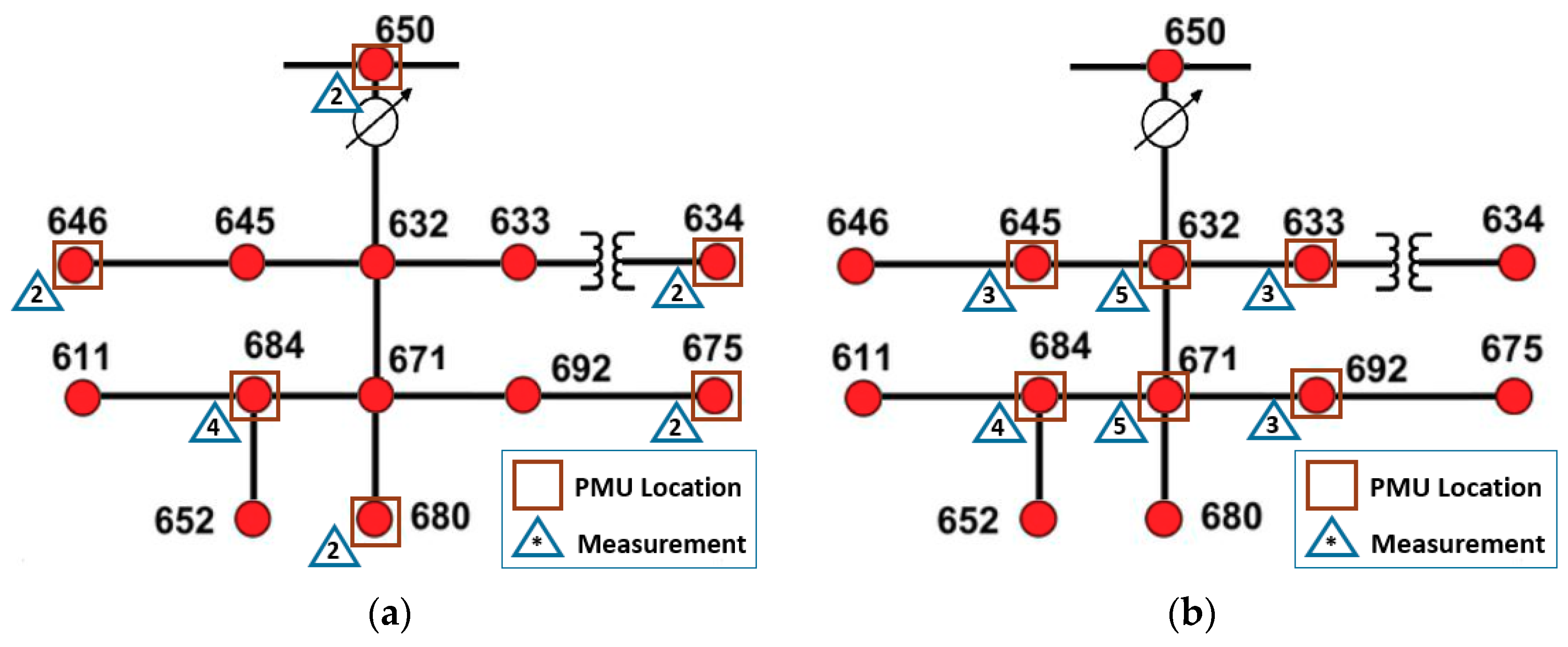
As can be seen, both BSA and MILP approaches ensured full grid observability of the test distribution feeders with an equal number of PMU installation. Besides, the BSA approach achieved more measurement redundancy over the MILP approach by rearranging the positions of the PMU among the nodes. For instance, Figure 2 presents the optimal locations of PMU and respective measurement redundancy employing the MILP and BSA approaches for the IEEE 13-node feeder. As can be observed, both approaches selected the node 684 for PMU installation that can make observable a total of four nodes (611, 652, 671, and 684). Hence, the MILP and BSA approaches achieved 14 and 23 measurement redundancy, respectively. Likewise, the MILP approach achieved 35, 43 and 132 whereas the BSA achieved 42, 47 and 169 measurement redundancies for the IEEE 34-node, 37-node, and 128-node test feeders, respectively. Consequently, the presented results illustrate the superiority of the BSA approach over the MILP approach in obtaining the global best solutions. Table 2 also presents the execution times of the MILP and BSA approaches. As can be observed, the BSA approach required relatively larger computational time compared to the MILP approach for the tested cases. However, the computational burden of the BSA approach can be ignored as the OPP formulation are solved offline before the installation of PMU and this research aimed to achieve the maximum number of measurement redundancy.

Table 3. Comparison of optimal numbers of PMU without considering ZIB and channel limits.

Method	IEEE 13-Node			IEEE 34-Node			IEEE 37-Node			IEEE 128-Node
	RNP 1	RMR 2	AMR 3	RNP	RMR	AMR	RNP	RMR	AMR	RNP	RMR	AMR
Proposed (BSA)	6	13	23	12	34	42	12	37	47	48	128	169
MILP	6	13	14	12	34	35	12	37	43	48	128	132
Two-stage [31]	6	-	-	13	-	-	-	-	-	49	-	-
ILP [31]	6	-	-	12	-	-	-	-	-	48	-	-

¹ RNP: Required number of the PMU; ² RMR: Required measurement redundancy; ³ AMR: Achieved measurement redundancy.

compares the obtained results of the proposed OPP formulation with the results of the referenced works without considering the presence of ZIB and channel limitation of the available PMU. The optimal number of PMU required through the proposed formulation is equal to the minimum number of PMU recommended by the ILP method of Ref. [29] and less than to the minimum number of PMU recommended by the two-stage method of the same literature. As mentioned earlier, this research modified IEEE 123-node test feeder to 128-node feeder and still required the same or a smaller number of PMU installation to ensure full grid observability. Consequently, it can be concluded that the proposed BSA approach is more promising over the reported approaches in solving the formulated OPP problem. Additionally, the proposed approach ensured the maximum number of measurement redundancy whereas the reported methodologies did not consider the measurement redundancy issue. Besides, the reported OPP formulations for the distribution grids did not consider any contingency case, the inclusion of passive measurements and channel limitations of the PMU.

Table 4. Optimal numbers and locations of PMU without considering ZIB and channel limits during single line outage case.

Test Feeder	Method	No. of PMU	Locations of the PMU	Measurement Redundancy
				Required	Achieved
IEEE 13-node	MILP	7	632, 634, 645, 650, 671, 675, 684	20	23
	BSA	7	632, 633, 645, 650, 671, 684, 692		25
IEEE 34-node	MILP	19	800, 802, 808, 812, 814, 816, 818, 822, 824, 830, 832, 834, 836, 844, 846, 854, 858, 862, 890	59	62
	BSA	19	800, 802, 808, 812, 814, 816, 818, 820, 824, 830, 832, 834, 836, 844, 846, 854, 858, 862, 888		64
IEEE 37-node	MILP	18	701, 702, 704, 705, 707, 708, 709, 710, 711, 718, 720, 725, 727, 730, 734, 738, 744, 799	59	64
	BSA	18	701, 702, 703, 704, 705, 706, 707, 708, 709, 710, 711, 714, 720, 727, 734, 738, 744, 799		67
IEEE 128-node	MILP	73	1, 3, 6, 8, 9, 14, 15, 18, 20, 21, 24, 26, 27, 28, 29, 32, 34, 35, 36, 39, 41, 43, 44, 46, 47, 50, 51, 52, 54, 55, 58, 59, 60, 62, 64, 65, 67, 69, 70, 73, 74, 77, 78, 81, 82, 85, 86, 87, 90, 92, 93, 95, 97, 98, 100, 102, 103, 106, 107, 108, 110, 112, 114, 149, 150, 152, 195, 250, 251, 300, 450, 451, 610	219	230
	BSA	73	1, 3, 5, 8, 9, 14, 15, 18, 19, 21, 23, 26, 27, 28, 29, 31, 34, 35, 36, 38, 40, 42, 44, 45, 47, 50, 51, 52, 54, 55, 57, 58, 60, 61, 63, 64, 65, 67, 69, 70, 73, 74, 76, 77, 78, 81, 82, 84, 87, 89, 91, 93, 95, 97, 98, 100, 102, 103, 105, 106, 108, 110, 112, 113, 149, 150, 152, 195, 250, 251, 300, 450, 451		253

and

Table 5. Optimal numbers and locations of PMU without considering ZIB and channel limits during single PMU loss case.

Test Feeder	Method	No. of PMU	Locations of the PMU	Measurement Redundancy
				Required	Achieved
IEEE 13-node	MILP	13	611, 632, 633, 634, 645, 646, 650, 652, 671, 675, 680, 684, 692	26	37
	BSA	13	611, 632, 633, 634, 645, 646, 650, 652, 671, 675, 680, 684, 692		37
IEEE 34-node	MILP	27	800, 802, 808, 810, 814, 818, 820, 822, 824, 826, 830, 832, 834, 836, 838, 840, 844, 846, 848, 850, 854, 856, 858, 862, 864, 888, 890	68	78
	BSA	27	800, 802, 808, 810, 812, 814, 816, 820, 822, 824, 826, 830, 832, 834, 836, 838, 840, 842, 846, 848, 854, 856, 858, 862, 864, 888, 890		79
IEEE 37-node	MILP	31	701, 702, 703, 705, 706, 707, 708, 709, 710, 711, 712, 713, 714, 718, 722, 724, 725, 728, 729, 731, 732, 734, 735, 736, 738, 740, 741, 742, 744, 775, 799	74	89
	BSA	31	701, 702, 703, 704, 705, 706, 707, 708, 709, 710, 711, 712, 714, 718, 722, 724, 725, 728, 729, 731, 732, 734, 735, 736, 737, 740, 741, 742, 744, 775, 799		90
IEEE 128-node	MILP	103	1, 2, 3, 4, 5, 6, 8, 10, 11, 12, 13, 14, 15, 16, 17, 19, 20, 21, 22, 23, 24, 27, 28, 29, 31, 32, 33, 35, 36, 37, 38, 39, 40, 41, 42, 43, 45, 46, 47, 48, 50, 51, 52, 53, 55, 56, 58, 59, 60, 61, 63, 64, 65, 66, 67, 69, 70, 71, 72, 74, 75, 76, 78, 79, 81, 82, 83, 84, 85, 87, 88, 89, 90, 91, 92, 93, 94, 95, 96, 98, 99, 102, 103, 104, 105, 106, 107, 109, 110, 111, 113, 114, 135, 149, 150, 195, 250, 251, 300, 350, 450, 451, 610	256	300
	BSA	103	1, 2, 3, 4, 5, 6, 8, 10, 11, 12, 13, 14, 15, 16, 17, 18, 19, 20, 21, 22, 23, 24, 27, 28, 29, 31, 32, 33, 35, 36, 37, 38, 39, 40, 41, 42, 43, 45, 46, 47, 48, 50, 51, 52, 53, 54, 55, 56, 58, 59, 60, 61, 63, 64, 65, 66, 67, 69, 70, 71, 72, 74, 75, 76, 78, 79, 81, 82, 83, 84, 85, 87, 88, 89, 90, 91, 92, 93, 95, 96, 97, 99, 100, 101, 103, 104, 106, 107, 108, 110, 111, 113, 114, 149, 150, 195, 250, 251, 300, 350, 450, 451, 610		306

present the optimum number and locations of the PMU along with the required and the achieved measurement redundancies subjected to full grid observability of the selected test distribution feeders during single line outage and single PMU loss cases, respectively. Both approaches observed the test distribution feeders completely and the BSA achieved more or at least an equal number of measurement redundancy with an equal number of PMU installation. Consequently, the obtained results confirmed the superiority of the BSA approach over the MILP approach in terms of achieving measurement redundancy even for the contingency cases. However, this paper refrained from presenting the execution times in Table 4, Table 5,

Table 6. Optimal numbers and locations of PMU for different distribution test feeders during the normal operating mode considering ZIB only.

Test Feeder	Method	No. of PMU	Locations of the PMU	Measurement Redundancy
				Required	Achieved
IEEE 13-node	MILP	4	632, 645, 684, 692	10	15
	BSA	4	632, 645, 671, 692		16
IEEE 34-node	MILP	10	800, 808, 820, 824, 836, 844, 848, 854, 858, 862	29	33
	BSA	10	802, 808, 820, 824, 834, 836, 846, 854, 858, 862		36
IEEE 37-node	MILP	8	701, 709, 711, 714, 733, 734, 744, 799	26	28
	BSA	8	701, 702, 709, 710, 711, 714, 734, 744		32
IEEE 128-node	MILP	28	1, 5, 8, 13, 19, 30, 31, 38, 42, 45, 48, 49, 54, 55, 58, 62, 65, 70, 74, 76, 82, 84, 87, 95, 100, 103, 106, 113	91	95
	BSA	28	1, 5, 8, 18, 19, 30, 31, 38, 42, 45, 47, 50, 54, 55, 58, 62, 65, 70, 74, 76, 82, 84, 87, 95, 100, 103, 106, 113		97

,

Table 7. Optimal numbers and locations of PMU for different distribution test feeders under single line outage case considering ZIB only.

Test Feeder	Method	No. of PMU	Locations of the PMU	Measurement Redundancy
				Required	Achieved
IEEE 13-node	MILP	6	632, 645, 650, 675, 684, 692	18	19
	BSA	6	632, 645, 650, 671, 684, 692		22
IEEE 34-node	MILP	15	800, 802, 808, 818, 820, 824, 828, 832, 834, 836, 844, 846, 854, 858, 862	50	51
	BSA	15	800, 802, 808, 818, 820, 824, 828, 832, 834, 836, 844, 846, 854, 858, 862		51
IEEE 37-node	MILP	14	701, 702, 703, 707, 708, 709, 710, 711, 714, 727, 734, 738, 744, 799	49	52
	BSA	14	701, 702, 704, 705, 708, 709, 710, 711, 714, 727, 734, 738, 744, 799		52
IEEE 128-node	MILP	48	1, 3, 5, 8, 13, 18, 19, 25, 26, 28, 29, 31, 35, 38, 42, 45, 47, 49, 51, 54, 55, 58, 60, 62, 64, 65, 67, 69, 70, 73, 74, 76, 78, 81, 83, 85, 87, 95, 98, 99, 102, 103, 106, 112, 113, 195, 250, 450	162	166
	BSA	48	1, 3, 5, 8, 13, 18, 19, 21, 25, 28, 29, 31, 38, 42, 44, 45, 47, 49, 50, 54, 55, 58, 60, 62, 64, 65, 67, 69, 70, 73, 74, 76, 78, 81, 82, 84, 87, 95, 98, 99, 102, 103, 106, 112, 113, 195, 250, 450		168

,

Table 8. Optimal numbers and locations of PMU for different distribution test feeders under single PMU loss case considering ZIB only.

Test Feeder	Method	No. of PMU	Locations of the PMU	Measurement Redundancy
				Required	Achieved
IEEE 13-node	MILP	7	632, 645, 646, 650, 675, 684, 692	20	21
	BSA	7	632, 645, 646, 650, 675, 684, 692		21
IEEE 34-node	MILP	23	800, 802, 808, 810, 818, 820, 822, 824, 826, 828, 834, 836, 838, 840, 844, 846, 848, 854, 856, 858, 862, 864, 888	58	66
	BSA	23	800, 802, 808, 810, 816, 820, 822, 824, 826, 828, 832, 834, 836, 838, 840, 844, 846, 848, 854, 856, 858, 862, 864		68
IEEE 37-node	MILP	16	701, 702, 704, 705, 708, 709, 710, 711, 714, 718, 728, 729, 734, 738, 744, 799	52	55
	BSA	16	701, 702, 703, 705, 709, 710, 711, 714, 718, 720, 728, 729, 734, 738, 744, 799		55
IEEE 128-node	MILP	62	1, 2, 5, 6, 7, 8, 13, 14, 18, 19, 20, 28, 29, 31, 32, 38, 39, 42, 43, 45, 46, 47, 48, 49, 51, 54, 55, 56, 58, 59, 62, 63, 65, 66, 67, 68, 70, 71, 74, 75, 81, 82, 83, 84, 85, 86, 87, 88, 95, 96, 98, 100, 103, 104, 106, 107, 113, 114, 195, 250, 300, 450	182	184
	BSA	62	1, 2, 5, 6, 7, 8, 13, 18, 19, 20, 28, 29, 31, 32, 35, 38, 39, 42, 43, 45, 46, 47, 48, 50, 51, 54, 55, 56, 58, 59, 60, 62, 63, 65, 66, 67, 69, 70, 71, 74, 75, 76, 78, 82, 83, 84, 85, 87, 88, 95, 96, 98, 100, 103, 104, 106, 107, 113, 114, 195, 250, 450		186

,

Table 9. Optimal numbers and locations of PMU considering ZIB and a single channel for each PMU during a single PMU loss case.

Test Feeder	Method	No. of PMU	Locations of the PMU	Measurement Redundancy
				Required	Achieved
IEEE 13-node	MILP	10	632, 632, 645, 646, 650, 671, 671, 675, 680, 692	20	20
	BSA	10	632, 633, 645, 646, 650, 671, 675, 684, 684, 692		20
IEEE 34-node	MILP	30	800, 802, 802, 806, 808, 810, 816, 818, 820, 822, 824, 826, 828, 830, 834, 836, 838, 840, 842, 844, 846, 848, 854, 856, 858, 860, 862, 864, 888, 890	58	60
	BSA	30	800, 802, 802, 806, 808, 810, 818, 820, 820, 822, 824, 826, 828, 830, 834, 836, 838, 840, 842, 844, 846, 848, 852, 854, 856, 858, 860, 862, 864, 888		60
IEEE 37-node	MILP	27	701, 708, 708, 708, 709, 709, 709, 709, 711, 714, 718, 728, 729, 730, 731, 732, 733, 734, 735, 736, 737, 740, 741, 744, 744, 775, 799	52	54
	BSA	27	701, 708, 708, 708, 709, 709, 709, 709, 711, 714, 718, 728, 729, 730, 731, 732, 733, 734, 735, 736, 737, 740, 741, 744, 744, 775, 799		54
IEEE 128-node	MILP	91	1, 2, 5, 6, 19, 20, 28, 29, 31, 32, 38, 39, 40, 40, 41, 42, 42, 42, 43, 44, 44, 44, 45, 45, 46, 47, 47, 48, 49, 50, 52, 55, 56, 58, 59, 60, 62, 63, 64, 65, 66, 68, 69, 70, 71, 74, 75, 76, 81, 82, 82, 83, 84, 84, 85, 86, 87, 88, 95, 95, 96, 98, 99, 103, 104, 106, 107, 111, 112, 113, 114, 135, 135, 149, 149, 151, 151, 152, 152, 160, 160, 195, 250, 251, 300, 300, 300, 350, 450, 451, 610	182	182
	BSA	91	1, 2, 3, 5, 6, 13, 13, 13, 14, 18, 19, 19, 20, 21, 23, 25, 26, 27, 27, 29, 30, 31, 32, 36, 38, 39, 40, 42, 43, 44, 45, 46, 47, 47, 48, 50, 51, 53, 54, 55, 56, 58, 59, 60, 60, 60, 61, 62, 63, 64, 65, 66, 67, 68, 69, 70, 71, 74, 75, 76, 76, 77, 81, 82, 82, 83, 84, 85, 86, 87, 88, 89, 93, 94, 95, 95, 96, 97, 99, 100, 103, 104, 106, 107, 109, 113, 114, 149, 195, 250, 450		182

and

Table 10. Optimal numbers and locations of PMU during normal and contingency cases considering both ZIB and channel limits.

Test Feeder	Channel Limit	Method	Cases
			Normal Operation		Single Line Outage		Single PMU Loss
			RNP 1	AMR 1	RNP	AMR	RNP	AMR
IEEE 13-node	1	MILP	5	10	9	18	10	20
		BSA	5	10	9	18	10	20
	2	MILP	4	12	6	18	8	22
		BSA	4	12	6	18	8	22
	3	MILP	4	14	5	18	7	22
		BSA	4	14	5	18	7	22
	4	MILP	4	15	6	19	7	21
		BSA	4	16	6	22	7	21
	5	MILP	4	15	6	19	7	21
		BSA	4	16	6	22	7	21
IEEE 34-node	1	MILP	15	30	26	52	30	60
		BSA	15	30	26	52	30	60
	2	MILP	11	33	17	50	23	64
		BSA	11	33	17	50	23	65
	3	MILP	10	33	15	51	23	66
		BSA	10	36	15	51	23	68
	4	MILP	10	33	15	51	23	66
		BSA	10	36	15	51	23	68
	5	MILP	10	33	15	51	23	66
		BSA	10	36	15	51	23	68
IEEE 37-node	1	MILP	14	28	25	50	27	54
		BSA	14	28	25	50	17	54
	2	MILP	9	27	17	50	19	55
		BSA	9	27	17	50	19	55
	3	MILP	8	28	14	50	16	53
		BSA	8	30	14	50	16	53
	4	MILP	8	28	14	52	16	55
		BSA	8	32	14	52	16	55
	5	MILP	8	28	14	52	16	55
		BSA	8	32	14	52	16	55
IEEE 128-node	1	MILP	48	96	81	162	91	182
		BSA	46	92	81	162	91	182
	2	MILP	31	93	54	162	66	183
		BSA	31	93	4	162	66	183
	3	MILP	28	92	50	167	63	185
		BSA	28	93	49	164	63	186
	4	MILP	28	95	48	166	62	184
		BSA	28	97	48	168	62	186
	5	MILP	28	95	48	166	62	184
		BSA	28	97	48	168	62	186

¹ RNP: Required number of PMU; ² AMR: Achieved measurement redundancy.

as they are similar to the values of Table 2.

4.2. Full Grid Observability Considering the Presence of ZIB Only

Table 6 presents the optimum numbers and locations of the PMU along with the required and the achieved measurement redundancy subjected to the full observability of the selected distribution test feeders for normal operating mode after incorporation of passive measurements/ZIB. As can be observed, both solution methodologies, the BSA and MILP approaches confirmed grid observability through the installation of an equal number of PMU. The incorporation of ZIB on the selected test feeders reduced the required number of PMU significantly hence the installation and configuration costs can be compared from Table 6 and Table 2. For instance, the ratio of the required number of PMU to the total number of nodes (ψ) was reduced from 46.15% to 30.77%, 35.29% to 29.41%, 32.43% to 21.62% and 37.50% to 21.88% for normal operating mode of the selected IEEE 13-node, 34-node, 37-node and 128-node test distribution feeders, respectively. Additionally, the BSA approach achieved more measurement redundancy over the MILP approach for all the test distribution feeders.

Similarly, Table 7 and Table 8 present the optimum number and locations of the PMU along with the required and achieved measurement redundancies subjected to the full observability of the selected test distribution feeders during single line outage and single PMU loss cases, respectively.

The incorporation of the passive measurements on the selected test feeders reduced the required number of PMU significantly hence the installation and configuration costs, as can be compared from Table 7 and Table 4. For instance, the ratio, ψ got reduced from 53.58% to 46.15%, 55.88% to 44.12%, 48.65% to 37.84% and 57.03% to 37.50% for the single line outage case for the selected IEEE 13-node, 34-node, 37-node, and 128-node distribution feeders, respectively. However, both solution methodologies observed the test distribution feeders completely and the BSA achieved more or at least equal number of measurement redundancy through the installation of an equal number of PMU. Therefore, it can be concluded that the BSA approach was superior in figuring out the global optimal solution while solving the proposed OPP formulation over the MILP approach.

4.3. Full Grid Observability Considering Both ZIB and Channel Limits

This section considers the channel limitations of the available PMU along with the incorporation of ZIB while ensuring full grid observability of the selected test distribution feeders during both normal and contingency cases. Table 9 presents the required number of PMU and their locations along with the required and achieved numbers of measurement redundancies during a single PMU loss case considering single channel of the available PMU and the incorporation of the passive measurements.

As can be observed, some nodes required several PMU due to the availability of the least number of PMU channel. Additionally, the obtained results show both solution methodologies achieved full grid observability with an exactly same number of PMU installation. Besides, both approaches achieved only the required number of measurement redundancy as Table 9 presents the most severe contingency case with the minimum number of PMU channel. However, for brevity’s sake and to avoid repetition of similar tables and discussions, this paper refrained from presenting results of other operating cases by varying the channel limitations of the PMU, instead, all the cases have been summarized in Table 10. The locations of the PMU and the number of measurement redundancies for the presented simulated scenarios are omitted for brevity’s sake. As can be observed from Table 10, the BSA approach required an equal or a smaller number of PMU installation over the MILP approach to achieve the full grid observability for both normal and contingency cases. For instance, the BSA approach achieved full grid observability with a total of 46 PMU installation whereas the MILP approach required a total of 48 PMU installation having a single channel for the normal operating situation of IEEE 128-node distribution feeder. In addition, the BSA approach achieved more measurement redundancy over the MILP approach for many cases and at least an equal number of measurement redundancy for other cases with the same number of PMU installation. Hence, the obtained results confirmed the superiority of the BSA approach over the MILP approach in terms of achieving more measurement redundancy.

It can also be observed that the required number of PMU was reduced with the increase of available PMU channels to ensure full grid observability of the selected distribution test feeders. It is worth mentioning that the proposed OPP formulation and the solution methodologies required the same number of PMU installation to ensure full grid observability with the PMU having four or more channels. Hence, it is neither necessary nor economically viable to install PMU with more than four channels for the tested distribution feeders. The PMU manufacturers, as well as the decision-makers of power system monitoring, may find this conclusion useful while designing the wide area measurement and monitoring scheme problem considering channel limits of the available PMU.

5. Conclusions

This paper formulated a revised, effective and comprehensive OPP problem for the distribution grids through achievement of the maximum number of measurement redundancy with the installation of a minimal number of PMU. The formulation was extended considering the channel limitations of available PMU and presence of the passive measurement under various contingency cases related to electric distribution feeders, i.e., the single line outage and single PMU loss. This research solved the proposed OPP formulation employing an effective heuristic optimization approach called BSA. The results exhibited that the heuristic approach can ensure full grid observability with lower or at least an equal number of PMU installation than the MILP approach and other referenced works. Additionally, the results confirmed the superiority of the BSA approach over the MILP approach in terms of measurement redundancy. However, it is worth mentioning that the employment of PMU with more than four channels did not minimize the required number of PMU for the tested distribution feeders rather increased the investment cost.

References

- Kyritsis, E.; Andersson, J.; Serletis, A. Electricity prices, large-scale renewable integration, and policy implications. Energy Policy 2017, 101, 550–560. [Google Scholar] [CrossRef] [Green Version]
- Al-Mohammed, A.; Abido, M. A fully adaptive PMU-based fault location algorithm for series-compensated lines. IEEE Trans. Power Syst. 2014, 29, 2129–2137. [Google Scholar] [CrossRef]
- Shafiullah, M.; Al-Awami, A.T. Maximizing the profit of a load aggregator by optimal scheduling of day ahead load with EVs. In Proceedings of the IEEE International Conference on Industrial Technology, Seville, Spain, 17–19 March 2015. [Google Scholar] [CrossRef]
- Shafiullah, M.; Rahman, S.M.; Mortoja, M.G.; Al-Ramadan, B. Role of spatial analysis technology in power system industry: An overview. Renew. Sustain. Energy Rev. 2016, 66, 584–595. [Google Scholar] [CrossRef]
- Ochoa, L.F.; Wilson, D.H. Using synchrophasor measurements in smart distribution networks. In Proceedings of the 21st International Conference on Electricity Distribution CIRED 2011, Frankfurt, Germany, 6–9 June 2011; pp. 1–4. [Google Scholar]
- Muscas, C.; Pau, M.; Pegoraro, P.; Sulis, S. Smart electric energy measurements in power distribution grids. IEEE Instrum. Meas. Mag. 2015, 18, 17–21. [Google Scholar] [CrossRef]
- Abiri, E.; Rashidi, F.; Niknam, T. An optimal PMU placement method for power system observability under various contingencies. Int. Trans. Electr. Energy Syst. 2015, 25, 589–606. [Google Scholar] [CrossRef]
- Rashidi, F.; Abiri, E.; Niknam, T.; Salehi, M.R. Optimal placement of PMUs with limited number of channels for complete topological observability of power systems under various contingencies. Int. J. Electr. Power Energy Syst. 2015, 67, 125–137. [Google Scholar] [CrossRef]
- Abiri, E.; Rashidi, F.; Niknam, T.; Salehi, M.R. Optimal PMU placement method for complete topological observability of power system under various contingencies. Int. J. Electr. Power Energy Syst. 2014, 61, 585–593. [Google Scholar] [CrossRef]
- Chen, J.; Abur, A. Improved bad data processing via strategic placement of PMUs. In Proceedings of the IEEE Power Engineering Society General Meeting, San Francisco, CA, USA, 16 June 2005; pp. 2759–2763. [Google Scholar]
- Enshaee, A.; Hooshmand, R.A.; Fesharaki, F.H. A new method for optimal placement of phasor measurement units to maintain full network observability under various contingencies. Electr. Power Syst. Res. 2012, 89, 1–10. [Google Scholar] [CrossRef]
- Dua, D.; Dambhare, S.; Gajbhiye, R.K.; Soman, S.A. Optimal Multistage Scheduling of PMU Placement: An ILP Approach. IEEE Trans. Power Deliv. 2008, 23, 1812–1820. [Google Scholar] [CrossRef] [Green Version]
- Rahman, N.H.A.; Zobaa, A.F. Optimal PMU placement using topology transformation method in power systems. J. Adv. Res. 2016, 7, 625–634. [Google Scholar] [CrossRef] [PubMed]
- Al-Mohammed, A.H.; Abido, M.A.; Mansour, M.M. Optimal PMU placement for power system observability using differential evolution. In Proceedings of the 11th International Conference on Intelligent Systems Design and Applications, Cordoba, Spain, 22–24 November 2011; pp. 277–282. [Google Scholar]
- Shafiullah, M.; Rana, M.J.; Alam, M.S.; Uddin, M.A. Optimal placement of Phasor Measurement Units for transmission grid observability. In Proceedings of the 2016 International Conference on Innovations in Science, Engineering and Technology (ICISET), Dhaka, Bangladesh, 28–29 October 2016; pp. 1–4. [Google Scholar]
- Akhlaghi, S. Optimal PMU placement considering contingency-constraints for power system observability and measurement redundancy. In Proceedings of the 2016 IEEE Power and Energy Conference at Illinois (PECI), Urbana, IL, USA, 19–20 February 2016; pp. 1–7. [Google Scholar]
- Taher, S.A.; Mahmoodi, H.; Aghaamouei, H. Optimal PMU location in power systems using MICA. Alex. Eng. J. 2016, 55, 399–406. [Google Scholar] [CrossRef]
- Aminifar, F.; Khodaei, A.; Fotuhi-Firuzabad, M.; Shahidehpour, M. Contingency-Constrained PMU Placement in Power Networks. IEEE Trans. Power Syst. 2010, 25, 516–523. [Google Scholar] [CrossRef]
- Tai, X.; Marelli, D.; Rohr, E.; Fu, M. Optimal PMU placement for power system state estimation with random component outages. Int. J. Electr. Power Energy Syst. 2013, 51, 35–42. [Google Scholar] [CrossRef]
- Miljanić, Z.; Djurović, I.; Vujošević, I. Optimal placement of PMUs with limited number of channels. Electr. Power Syst. Res. 2012, 90, 93–98. [Google Scholar] [CrossRef]
- Manousakis, N.M.; Korres, G.N. Optimal PMU Placement for Numerical Observability Considering Fixed Channel Capacity—A Semidefinite Programming Approach. IEEE Trans. Power Syst. 2016, 31, 3328–3329. [Google Scholar] [CrossRef]
- Manousakis, N.M.; Korres, G.N. Semidefinite programming for optimal placement of PMUs with channel limits considering pre-existing SCADA and PMU measurements. In Proceedings of the 2016 Power Systems Computation Conference (PSCC), Genoa, Italy, 20–24 June 2016; pp. 1–7. [Google Scholar]
- Sexauer, J.; Javanbakht, P.; Mohagheghi, S. Phasor measurement units for the distribution grid: Necessity and benefits. In Proceedings of the 2013 IEEE PES Innovative Smart Grid Technologies Conference (ISGT), Washington, DC, USA, 24–27 February 2013; pp. 1–6. [Google Scholar]
- Abdelaziz, A.Y.; Mohammed, F.M.; Mekhamer, S.F.; Badr, M.A.L. Distribution Systems Reconfiguration using a modified particle swarm optimization algorithm. Electr. Power Syst. Res. 2009, 79, 1521–1530. [Google Scholar] [CrossRef]
- Mekhamer, S.F.; Abdelaziz, A.Y.; Mohammed, F.M.; Badr, M.A.L. A new intelligent optimization technique for distribution systems reconfiguration. In Proceedings of the 2008 12th International Middle-East Power System Conference, Aswan, Egypt, 12–15 March 2008; pp. 397–401. [Google Scholar]
- Enacheanu, B.; Raison, B.; Caire, R.; Devaux, O.; Bienia, W.; Hadjsaid, N. Radial network reconfiguration using genetic algorithm based on the matroid theory. IEEE Trans. Power Syst. 2008, 23, 186–195. [Google Scholar] [CrossRef]
- Tahabilder, A.; Ghosh, P.K.; Chatterjee, S.; Rahman, N. Distribution system monitoring by using micro-PMU in graph-theoretic way. In Proceedings of the 2017 4th International Conference on Advances in Electrical Engineering (ICAEE), Dhaka, Bangladesh, 28–30 September 2017; pp. 159–163. [Google Scholar]
- Abdelsalam, H.A.; Abdelaziz, A.Y.; Osama, R.A.; Salem, R.H. Impact of distribution system reconfiguration on optimal placement of phasor measurement units. In Proceedings of the 2014 Clemson University Power Systems Conference, Clemson, SC, USA, 11–14 March 2014; pp. 1–6. [Google Scholar]
- Jamil, E.; Rihan, M.; Anees, M.A. Towards optimal placement of phasor measurement units for smart distribution systems. In Proceedings of the 6th IEEE Power India International Conference (PIICON), Delhi, India, 5–7 December 2014; pp. 1–6. [Google Scholar]
- Liu, J.; Tang, J.; Ponci, F.; Monti, A.; Muscas, C.; Pegoraro, P.A. Trade-Offs in PMU Deployment for State Estimation in Active Distribution Grids. IEEE Trans. Smart Grid 2012, 3, 915–924. [Google Scholar] [CrossRef]
- Liu, J.; Ponci, F.; Monti, A.; Muscas, C.; Pegoraro, P.A.; Sulis, S. Optimal Meter Placement for Robust Measurement Systems in Active Distribution Grids. IEEE Trans. Instrum. Meas. 2014, 63, 1096–1105. [Google Scholar] [CrossRef]
- Tran, V.; Zhang, H.; Nguyen, V. Optimal PMU Placement in Multi-configuration Power Distribution Networks. Adv. Comput. Sci. Res. 2016, 50, 508–514. [Google Scholar]
- Wang, H.; Zhang, W.; Liu, Y. A Robust Measurement Placement Method for Active Distribution System State Estimation Considering Network Reconfiguration. IEEE Trans. Smart Grid 2016, 1–12. [Google Scholar] [CrossRef]
- Koutsoukis, N.C.; Manousakis, N.M.; Georgilakis, P.S.; Korres, G.N. Numerical observability method for optimal phasor measurement units placement using recursive Tabu search method. IET Gener. Transm. Distrib. 2013, 7, 347–356. [Google Scholar] [CrossRef]
- Marinescu, R.; Dechter, R. AND/OR Branch-and-Bound for Solving Mixed Integer Linear Programming Problems. In Principles and Practice of Constraint Programming—CP 2005; Springer: Berlin/Heidelberg, Germany, 2005; p. 857. [Google Scholar]
- Civicioglu, P. Backtracking Search Optimization Algorithm for numerical optimization problems. Appl. Math. Comput. 2013, 219, 8121–8144. [Google Scholar] [CrossRef]
- Shafiullah, M.; Rana, M.J.; Coelho, L.S.; Abido, M.A.; Al-Subhi, A. Designing Lead-Lag PSS Employing Backtracking Search Algorithm to Improve Power System Damping. In Proceedings of the 9th IEEE-GCC Conference and Exhibition (GCCCE), Manama, Bahrain, 8–11 May 2017; pp. 1–6. [Google Scholar]
- Shafiullah, M.; Abido, M.A.; Coelho, L.S. Design of robust PSS in multimachine power systems using backtracking search algorithm. In Proceedings of the 2015 18th International Conference on Intelligent System Application to Power Systems (ISAP), Porto, Portugal, 11–16 September 2015; pp. 1–6. [Google Scholar]
- Kılıç, U. Backtracking search algorithm-based optimal power flow with valve point effect and prohibited zones. Electr. Eng. 2015, 97, 101–110. [Google Scholar] [CrossRef]
- Shafiullah, M.; Ijaz, M.; Abido, M.A.; Al-Hamouz, Z. Optimized support vector machine & wavelet transform for distribution grid fault location. In Proceedings of the 2017 11th IEEE International Conference on Compatibility, Power Electronics and Power Engineering (CPE-POWERENG), Cadiz, Spain, 4–6 April 2017; pp. 77–82. [Google Scholar]
- Distribution Test Feeders. Available online: https://ewh.ieee.org/soc/pes/dsacom/testfeeders/ (accessed on 18 September 2018).
Figure 1.
The flowchart for the backtracking search algorithm (BSA).
Figure 2.
The BSA and MILP based PMU locations and achieved measurement redundancy. (a) MILP based PMU locations; (b) BSA based PMU locations.