Quantifying the Nonlinear Dynamic Behavior of the DC-DC Converter via Permutation Entropy

Abstract

Quantifying nonlinear dynamic behaviors, such as bifurcation and chaos, in nonlinear systems are currently being investigated. In this paper, permutation entropy is used to characterize these complex phenomena in nonlinear direct current-direct current (DC-DC) converter systems. A mode switching time sequence (MSTS), containing the information from different periodic states, is obtained in a DC-DC converter by reading the inductor current when altering the switching mode. To obtain the nonlinear characteristics of this system, the concept of permutation entropy of symbolic probability distribution properties is introduced and the structure of the chaotic system is reproduced based on the theory of phase space reconstruction. A variety of nonlinear dynamic features of the DC-DC converter are analyzed using the MSTS and permutation entropy. Finally, a current-mode-controlled buck converter is reviewed as a case to study the quantification of nonlinear phenomena using permutation entropy as one of the system parameters changes.

1. Introduction

1.1. Background

Direct current-direct current (DC-DC) switching converters are a typical nonlinear system that enable the observation of nonlinear behaviors, such as period-doubling bifurcation, border collision bifurcation, frequency-locking phenomenon, quasi-period, and chaos [1,2,3,4,5]. The study of nonlinear behaviors is helpful for improving the performance of DC-DC converters.

1.2. Formulation of the Problem of Interest for This Investigation

Generally speaking, these nonlinear phenomena can be observed by phase plane, bifurcation diagrams, and Poincaré sections in DC-DC converters [6,7,8], but these only provide qualitative analyses. To examine nonlinear phenomena in a timely manner and identify them accurately, quantitative analysis is necessary. At present, some quantitative analysis methods have been proposed to process these nonlinear features, and the largest Lyapunov exponent (LLE) is the most common [9,10].

1.3. Literature Survey

In practical applications, analyzing the diverse nonlinear phenomena in LLE is challenging due to the complex of the phase space trajectory and its solution process is complicated [7,11]. Researchers [12] found the symbolic time sequence contains a large amount of DC-DC converter system state information, including nonlinear stability, bifurcation information, and degree of confusion. Both symbolic sequence analysis and entropy are utilized to quantitatively analyze DC-DC converters. Multiscale entropy and sample entropy are used to characterize nonlinear phenomena and fault features [13,14,15,16]. The symbolic time sequence method has been combined with block entropy to quantify bifurcation and chaos state in boost converters [12,17]. Switch information sequences and the concept of joint entropy have been used to quantify the complex state of the Ćuk converter [18,19].

1.4. Scope and Contribution of This Study

When the circuit parameters or the control parameters of the DC-DC converter are changed, the system tends to exhibit processes from bifurcation to chaos or other nonlinear behaviors. The conventional time sequence of a DC-DC converter is based on discrete mapping modeling with the control period as the sampling period, so the information of the switching state time is ignored. With nonlinear behavior, the switching state of a DC-DC converter may differ greatly in adjacent control periods. Therefore, this paper introduces the mode switching time sequence (MSTS) by sampling the value of the state variables at the mode switching moment. The MSTS not only obtains the modality of each period, but also distinguishes the modalities presented in different periods. Hence, two characteristics of the DC-DC converter can be simultaneously obtained through a time sequence period.

In traditional symbolic sequence analysis, the process of hierarchical symbolization is prone to excessive symbol in a certain layer, and the overlapping symbols indirectly lead to the loss of information. Permutation entropy [20,21] is a special symbol sequence method based on information entropy [22] and phase space reconstruction theory. It can effectively quantify the complexity of a time sequence. Permutation entropy does not need to stratify the amplitude of the time sequence, which is different from the general symbol sequence analysis method.

Permutation entropy is based on sorting the coordinates of the reconstructed phase space, and then the generated symbol space is compared with all possible symbol sequences to achieve classification. Permutation entropy can accurately obtain the autocorrelation degree of the time sequences [23,24]. When the sequence representation is completely random, the self-similarity of the sequence is zero. This implies that the probability of occurrence of each sequence is the same, and the entropy value is the largest. The entropy value is the smallest for the sequence based on a period-1 orbit because the sampling data in each period remain unchanged.

1.5. Organization of the Paper

This paper is organized as follows: Section 2 introduces the MSTS to describe the characteristics of the DC-DC converter. In Section 3, the identification of permutation entropy in periodic signals and the selection of parameters of permutation entropy are discussed. In Section 4, MSTS combined with permutation entropy is proposed. In Section 5, an example of a DC-DC converter is described in detail, and the proposed method is applied to analyze nonlinear behaviors. Finally, through discussion and summary, the feasibility of the method is demonstrated by comparison with other methods and the nonlinear dynamic behaviors of the DC-DC converter are better quantified.

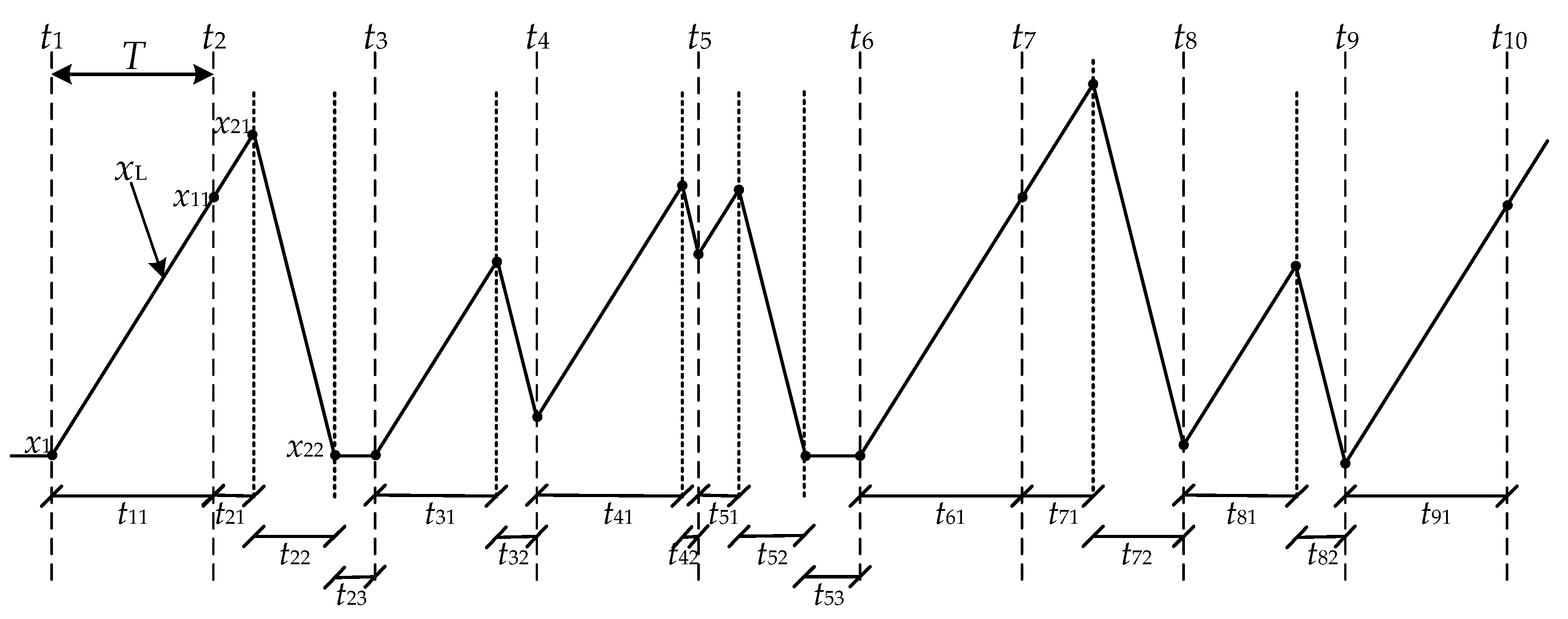
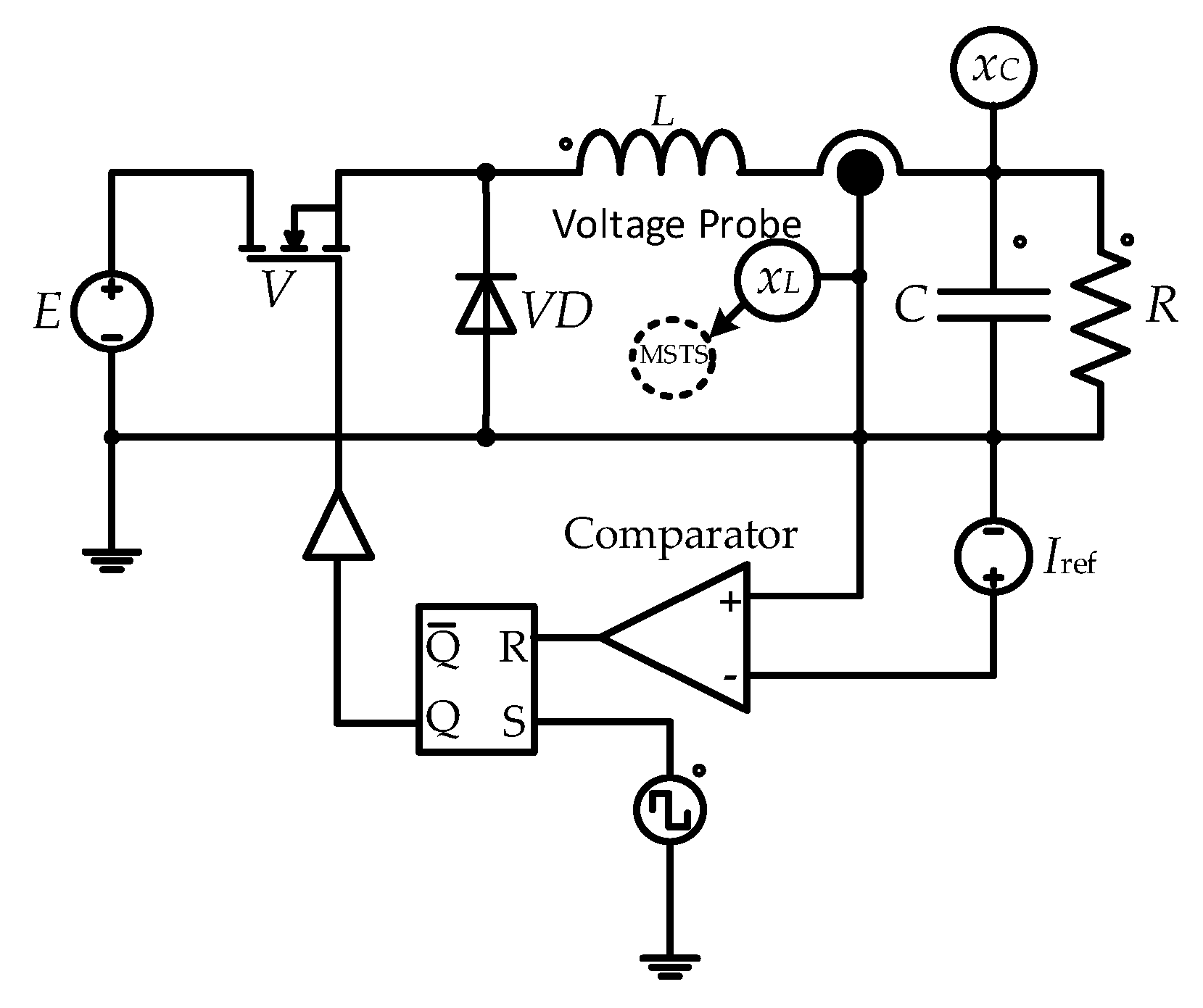
2. MSTS of the Modeled Converter

Current symbolic time sequence uses the control period as the sampling period in DC-DC converters. However, the switching states or the change in the system topology may be different in one control period, and the sampling control period ignores these details. For example, continuous conduction mode (CCM) and discontinuous conduction mode (DCM), both working in period-1, orbit at the stable state of the converter. So, the MSTS of the DC-DC converter is introduced to solve this issue and is shown as follows.

Set $X={[X_1{X}_2{X}_3\cdots X_p]}^{\mathrm{T}}$ to the state vector (with p being the numbers of variables and superscript T denoting transposition) of a DC-DC converter. So, in the ith control period, the discretized expression of X can be expressed as:

$$\{\begin{array}{l}X(t_i+t_{i1}+t_{i2}+\cdots +t_{ik})=S_k(X(t_i+t_{i1}+t_{i2}+\cdots +t_{i(k-1)}),t_{ik}),\\ X_{ik}=S_k(X_{i(k-1)},t_{ik}),\end{array}$$

(1)

where S_k represents the relationship between the nitial and final terative alues in the circuit topology as the operating mode k is presented (with its expression being only related to the topology and the selected state variable). t_i and t_ik represent the start time of the ith period and the mode k occurs in the period, and $X_{ik}=X(t_i+t_{i1}+t_{i2}+\cdots +t_{ik})$.

Suppose the system has j_i (1 ≤ j_i ≤ 2^m –1, where m indicates the number of switching devices) modes in the ith control period. As the system stabilizes, we take x_L in the state variable X as the object of observation and sample it when the mode changes from each control period. Hence, we obtain the MSTS, i.e.,

$$x_{L-\mathrm{MSTS}}=\{x_1,x_{11},x_{12},\dots ,x_{1j_1},x_{21},\dots ,x_{(N-1)j_{(N-1)},}{x}_{N1},x_{N2},\dots ,x_{N{j}_N}\},$$

(2)

Considering the equation $x(t_{i+1})=x(t_i+t_{i1}+\dots +t_{i{j}_i})$, the x_i+1 has to be left out from Equation (2). Figure 1 shows an example of two switching devices existing in the converter system, which means it can express up to three modes, where T is the control period and t_i is the time of the ith switching moment (t_i−t_i-1 = T).

3. Permutation Entropy

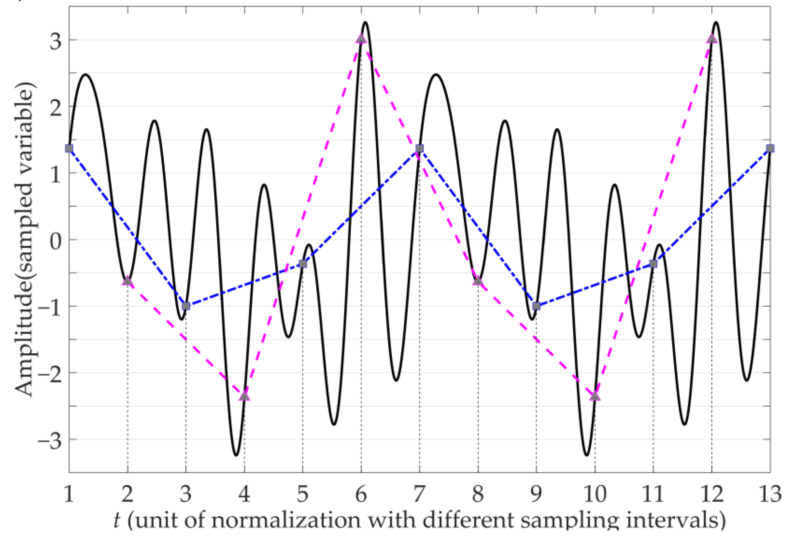
3.1. Phase Space Reconstruction Theory

The low-dimensional coordinate system cannot reflect the complex nonlinear states, as demonstrated by Packard et al. [25]. Packard et al. [25] proposed two methods of reconstructing phase space in a time sequence. The coordinate delay reconstruction method is widely used. In this method, the one-dimensional time sequence is constructed by embedding the dimension m and the delay time τ to form a new m-dimensional vector sequence. The phase space of the discrete time sequence x(n) of length N can be obtained:

$$Y(i)=\{x(i),x(i+\tau ),\dots ,x(i+\tau \times (m-1))\},i=1,2,\dots N-(m-1)\times \tau$$

(3)

Afterward, the Takens embedding theorems [26] proves the rationality of phase space reconstruction and proposes that the embedding dimension of phase space should satisfy m ≥ 2D + 1, where D is the singular attractor dimension of the system and it is a geometric invariant. A dynamic system with correlation dimension D can be described through 2D + 1 independent variables at most [7]. This means that the geometry of the dynamic system is completely open when m is greater than the minimum embedding dimension 2D + 1. At this time, the geometric invariant properties of the system, such as the Lyapunov exponent, are independent of the embedding dimension m. In addition, the delay time can be obtained by the autocorrelation method. The time sequence of a state variable can reconstruct the phase space of the system, for it contains information about all variables participating in the dynamic system. According to the Takens embedding theorem, the m-dimensional state space, expressed in Equation (4), has the same meaning as the original state space topologically; that is, the original state variable information can be reproduced.

$$Y=\left[\begin{array}{c}Y(1,:)\\ Y(2,:)\\ ⋮\\ Y(i,:)\\ ⋮\\ Y(N-(m-1)\times \tau ,:)\end{array}\right]=\left[\begin{array}{cccc}{x}_1& x_{1+\tau }& \dots & x_{1+\tau \times (m-1)}\\ x_2& x_{2+\tau }& \dots & x_{2+\tau \times (m-1)}\\ ⋮& ⋮& & ⋮\\ x_i& x_{i+\tau }& \dots & x_{i+\tau \times (m-1)}\\ ⋮& ⋮& & ⋮\\ x_{N-(m-1)\times \tau }& x_{N-(m-2)\times \tau }& \dots & x_N\end{array}\right]$$

(4)

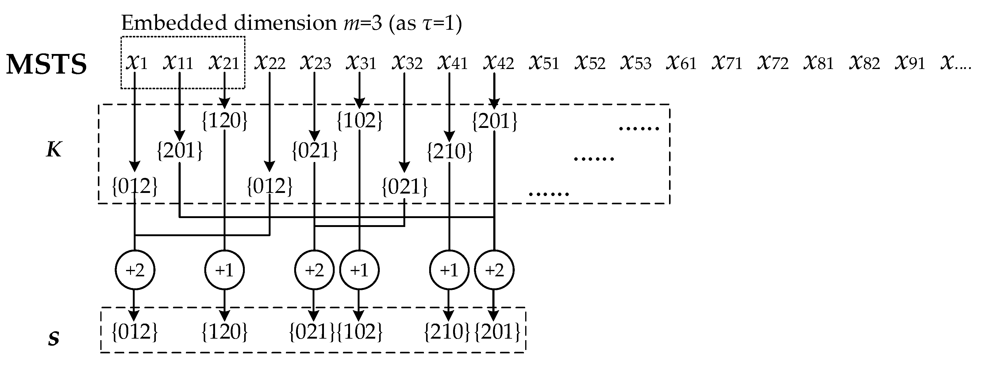
3.2. Symbol Permutation Method

Entropy can quantify the periodic states and chaos by time sequence. Its concept is sourced in the second law of thermodynamics. After Shannon introduced it into information theory, Shannon entropy became an important quantitative means to measure the probability distribution of a sequence signal [22].

For any discrete sequence $\{x(i),i=1,2,\dots ,n\}$, the corresponding probability distribution $\{p(i)|i=1,2,\dots ,n\}$ can be calculated, where p(i) is equal to the proportion of x(i) in the entire sequence. The Shannon entropy H_P can be defined as $H_{\mathrm{P}}=-{\displaystyle \sum p(i)}\ln p(i)$. The larger the H_P, the more uneven the signal distribution. This indicates that the system is highly complex, and the time sequence is difficult to predict. On the contrary, the information contained in the signal is easy to find for small H_P, and the prediction can be realized with minimal error. Particularly, in the case where H_P = 0, the sequence signal could be theoretically predictable, such as the step signal at t > 0.

In order to accurately quantify the nonlinear features, we first need to acquire certain statistical characteristics of the signal. In 2001, Bant et al. proposed the concept of permutation entropy based on phase space reconstruction theory, and successfully applied it to the complex quantization process of time sequences [23]. Equation (5) was generated by sorting Equation (4) in ascending order:

$$Y(i)=\{x(i+k_{i1}\tau )\le x(i+k_{i2}\tau )\le \dots \le x(i+k_{im}\tau )\}.$$

(5)

We determined the corresponding symbol permutation:

$$K_i=\{k_{i1},k_{i2},\dots ,k_{im}\},k_{i·}=0,1,\dots ,m-1.$$

(6)

For m-dimensional phase space reconstruction, we studied all n! permutations $s(g)$ of $\left(1,2,\dots ,m-1\right)$

$$s(g)=\{g_1,g_2,\dots ,g_m\},1<g<m!,$$

(7)

where $g_i\in (0,1,\dots ,m-1)(g_i\ne g_j,1\le i\le m,1\le j\le m)$. Then, comparing K_i logically with the sequence of symbols $s(g)$, we define p(g) as the probability that s(g) appears in $\{K_1;K_2;\dots ;K_{N-(M-1)\tau }\}$:

$$p(g)=\frac{Card\{i|1\le i\le N-(m-1)\tau ,K_i==s(g)\}}{m!},$$

(8)

where Card is a function that represents the number of elements in a collection

According to the definition of the Shannon entropy, the permutation entropy can be defined as:

$${{\displaystyle PE}}^{(m)}=-{\displaystyle \sum _{g=1}^{m!}p(g)\ln p(g)}.$$

(9)

The whole -process -can be illustrated by the special example in Figure 2. In this graph, a sequence of period-6 was chosen as the object of analysis below. We set the embedding dimension m = 3 and the delay time τ = 2. It was assumed that the sequence is sampled from the first 13 data points onto the curve shown in Figure 2. In this case, the state space is divided into 3! (=6) parts, so there are 6 mutually different arrangement symbols. According to the definition in Equation (3), the first sample point has a three-dimensional (3D) coordinate of (1.3660,–1.0000,−0.3660). Following Equation (5), we found that x(i + τ) ≤ x(i + 2τ) ≤ x(i), i = 1. Then, the corresponding permutation is (−1.0000,−0.3660,1.3660) and the corresponding symbol sequence {120} is obtained by referring to Equation (6). Therefore, combined with Equation (3), the sequence (1.3660,−0.6340,−1.0000,−2.3660,−0.3660,3.0000,1.3660,−0.6340,−1.0000,−2.3660,−0.3660,3.0000,1.3660) can be converted into 9 symbol sequences for representation ({120}, {102}, {012}, {021}, {201}, {210}, {120}, {102}, {012}).

As analyzed above, the previous six symbol sequences are different from each other. Starting from the seventh symbol sequence, the periodic extension is performed in the order in which the first six sequences appeared. This means that all possible symbol sequences are included. The remaining other parameters are unchanged, the analysis is performed again with m = 4, and the above calculation is repeated to obtain 7 symbol sequences ({1230},{1032},{3012},{3021},{2031},{2130},{1230}). We considered $k_{ij}>k_{i(j+1)}$ as $x(i+k_{ij})=x(i+k_{i(j+1)})$. The permutation entropy calculated by Equation (8) is approximately 1.7918, provided the sampling sequence is long enough. The comparison shows that the distribution of symbol sequences in $m=3$ is consistent with $m=4$. That means if the cycle count is less than m!, the m would not affect the amount of information acquired. So, the information that can be obtained is also uniform.

The permutation entropy is a method proposed according to the spatial characteristics of time. We can obtain the new state space Y by reconstructing the phase space. After sorting each m-dimensional vector in Y, N − (m − 1)τ sorts symbol sequence K can be obtained. For the embedding dimension m, the total number of corresponding order permutations is m!. To ensure the degree of uniformity of quantization, N − (m − 1)τ >> m! is generally required, and N >> m! is adopted in practical application. Furthermore, if m is small, the signal with a higher multiple periodic cannot be identified. Hence, the information volume read is correspondingly reduced, eventually resulting in a loss of information. However, if the selection of m is oversized, it often leads to N < m!. As a consequence, the identification accuracy decreases and the error trend increases.

The noise-free chaotic sequence studied by Taken’s theorem of embedding indicates that there is no specific limitation on the delay time τ. τ does not take the optimal delay time only affects the Euclidean geometry of the reconstructed attractor when reconfiguring the phase space. So, it affects the calculation of the correlation dimension. However, it will not affect the reconstructive attractor’s unambiguous representation of the system dynamics. In addition, a completely independent situation of the two adjacent coordinate components could occur if the value of τ is too large, in which case, the projection of the chaotic attractor’s trajectory in the same direction would become irrelevant. Hence, smaller values of τ should be chosen according to the specific situation; Bandt and Pompe suggested choosing a τ value of 1 [20]. Therefore, the embedding dimension m is considered to be a key parameter of spatial reconstruction, and it is commonly recommended to select m within the range of 3 to 7 for systems with less than three dimensions.

The traditional symbol sequence divides the time sequence into n regions by amplitude coarse granulation to obtain the symbol sequence. After the window with length L is selected, the block entropy (BE) of the symbol sequence is obtained and its maximum value is not more than $\ln (2^L)$. For the permutation entropy, after the m-dimensional phase space reconstruction, the maximum value of the permutation entropy does not exceed $\ln (m!)$. That is to say, $m!>>2^L$ as $m=L>3$. Compared with the traditional symbol sequence method, the permutation entropy can read more information and does not need to perform amplitude layering. The method of combination of the permutation entropy and MSTS is elaborated in Section 4. Combined with MSTS, we compare permutation entropy and sample entropy in Section 5. Given the logical calculation used in the method, the permutation entropy has the advantages of high robustness and fast calculation speed.

4. Combination of MSTS and Permutation Entropy

In common DC-DC switching converters that include both an inductor and a capacitor, the trend in the current variable or voltage variable can reflect the operating mode of the system. For a switched capacitor DC-DC converter [27], since it does not contain an inductor, the capacitor voltage can be used as an object for extracting the MSTS. Peak current single loop control is characterized by the inability to stabilize the output voltage and produces a rich nonlinear behavior. We used the current variable as the observation signal for the common converter (Figure 1). The procedure of K as m = 3, τ = 1 can be observed in Figure 3.

Combined with the above analysis, the permutation entropy has the following characteristics when applied to a DC-DC converter:

(1)

Assuming the signal is random, such as white noise, permutation entropy is expected to be close to the maximum value $\ln (m!)$. Considering that there are at least two operation modes in period-1, the recurring number of the MSTS is greater than or equal to 2. Hence, the minimum value of PE is $\ln (2)=0.6931$.

(2)

When the system does not enter the chaotic state by changing m, the acquired permutation entropy remains uniform. This means that increasing or decreasing m as appropriate does not affect the value of the permutation entropy.

(3)

DCM and CCM can be further divided into different working patterns according to the different switching numbers of modes. Border collision occurs when the working pattern combination changes. The complexity of the systems in DCM working patterns is usually greater than that of the CCM working pattern. Therefore, the more DCM patterns the system contains, the higher the value of the permutation entropy. After entering chaos, the permutation sequence K shows a certain disorder. Because the chaotic motion is pseudo-random, the permutation entropy obtained in the chaotic state is not able to reach the maximum value.

5. Application Example

In this section, the peak current control buck DC-DC converter is analyzed using the above method. By quantifying its complexity, the behaviors of the period-doubling bifurcation, border collision bifurcation, and chaos present in the converter are quantitatively described. The circuit model is shown in Figure 4. Relevant parameters were selected as follows: E = 20 V, R = 19 Ω, L = 3.3 mH, C = 1000 uF, T = 400 us, and the variation range of the control variable I_ref was controlled within 0.12–1.32. As shown in Figure 4, there are two switching devices in the circuit: the fully controlled device V and the uncontrollable diode VD. Combined with the principle of the buck converter, we obtained three working modes of the circuit, as shown in Figure 5 and Figure 6. These figures depict the switching mode (V,VD) = (on,off)→(V,VD) = (off,on)→(V,VD) = (off,off) of each switching period. The inductor current is x_L > 0 during mode-1 and mode-2 and x_L = 0 during mode-3. In Figure 6, Ib₁ and Ib₂ are the borderlines in the buck converter with peak current control. Analyzing the characteristics of the buck converter and using the precise discretization method to model the system, we determined the work pattern of each control cycle. After multiple iterations, the inductor current x_L was numerically sampled under the overall steady state, and MSTS was obtained. Here, m = 4 and τ = 1 were selected. Figure 7 shows the permutation entropy for the MSTS as a function of the reference current for different nonlinear feature. For the data of the chaotic state part, since the irregularity was relatively strong, cycle extension was performed to homogenize the order.

As shown in Figure 8, the inductor current x_L is sampled at the operating mode interval and the bifurcation diagram of the system with I_ref as a changing parameter can be obtained.

By comparing Figure 7 and Figure 8, the dynamic behavior of the buck converter in the peak current control can be clearly analyzed. Similarly, each state of the border collision bifurcation and the standard bifurcation are represented in

Table 1. Permutation sequence and permutation entropy of the buck converter as reference current I_ref changes.

Iref/A	S	MSTS-PE	State
[0.1200,0.2778]	({1203},{0231},{0231})∞	1.0986	Period-1
[0.2779,0.8295]	({1203},{0213})∞	0.6931	Period-1
[0.8296,0.9006]	({3102},{2013},{1302},{0213})∞	1.3863	Period-2
[0.9007,1.1577]	({3102},{2301},{1203},{0132},{0213})∞	1.6094	Period-2
[1.1578,1.1946]	({2301},{1230},{0123},{0312})∞	1.3863	Period-2
[1.1947,1.2624]	({2031},{1203},{3012},{2301},{1230},{0123},{0312})∞	1.9459	Period-4
[1.2625,1.3200]	No period: ({…}, …)	>2.2	Chaos

. In this table, S and MSTS-PE indicate the permutation symbol of the MSTS and the corresponding permutation entropy, respectively.

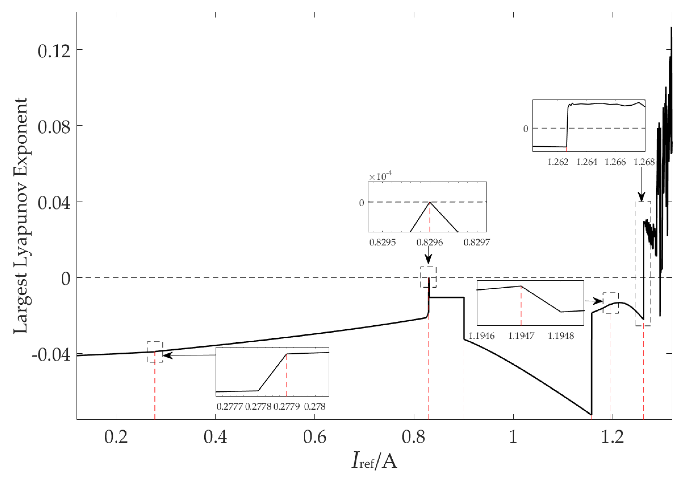
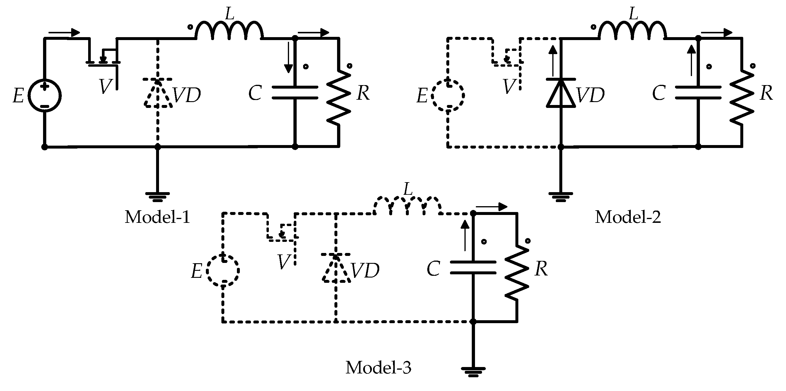
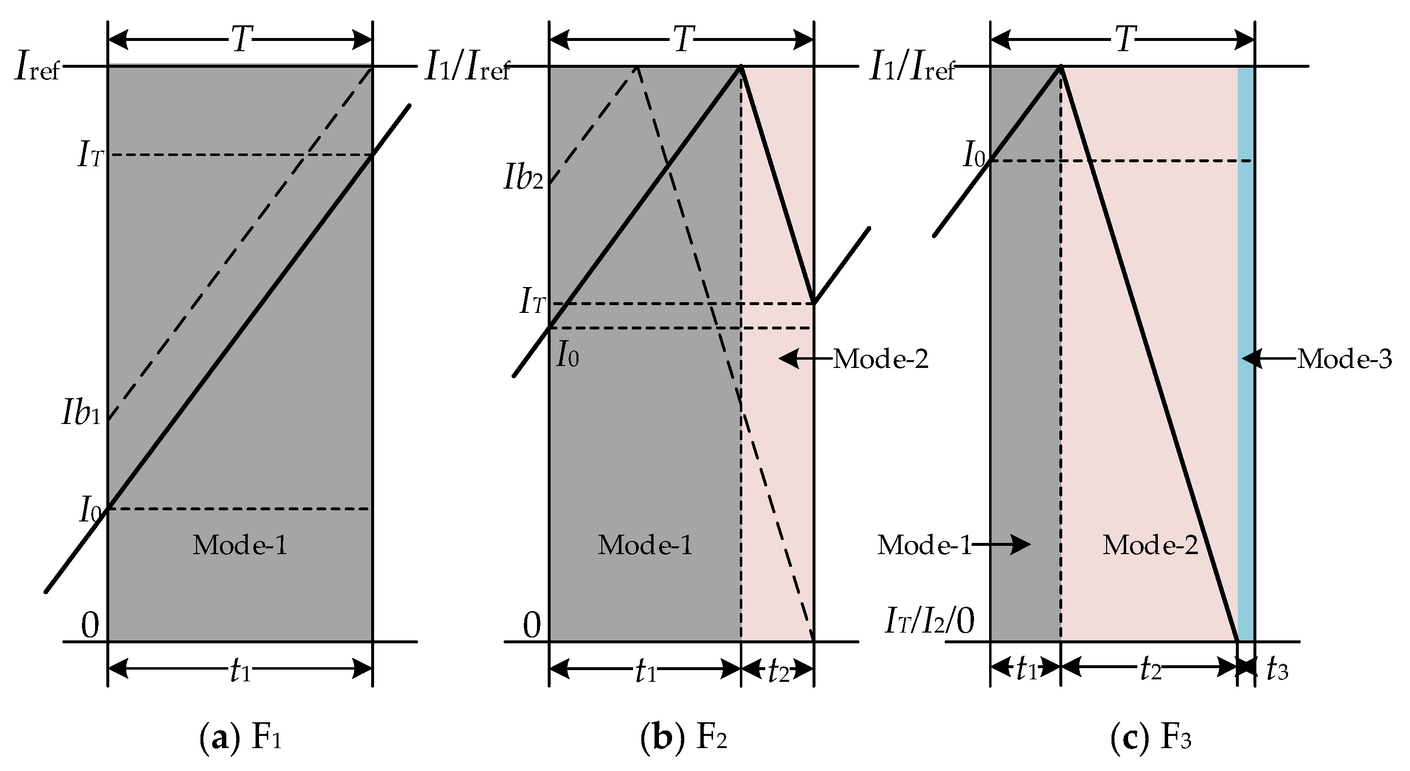
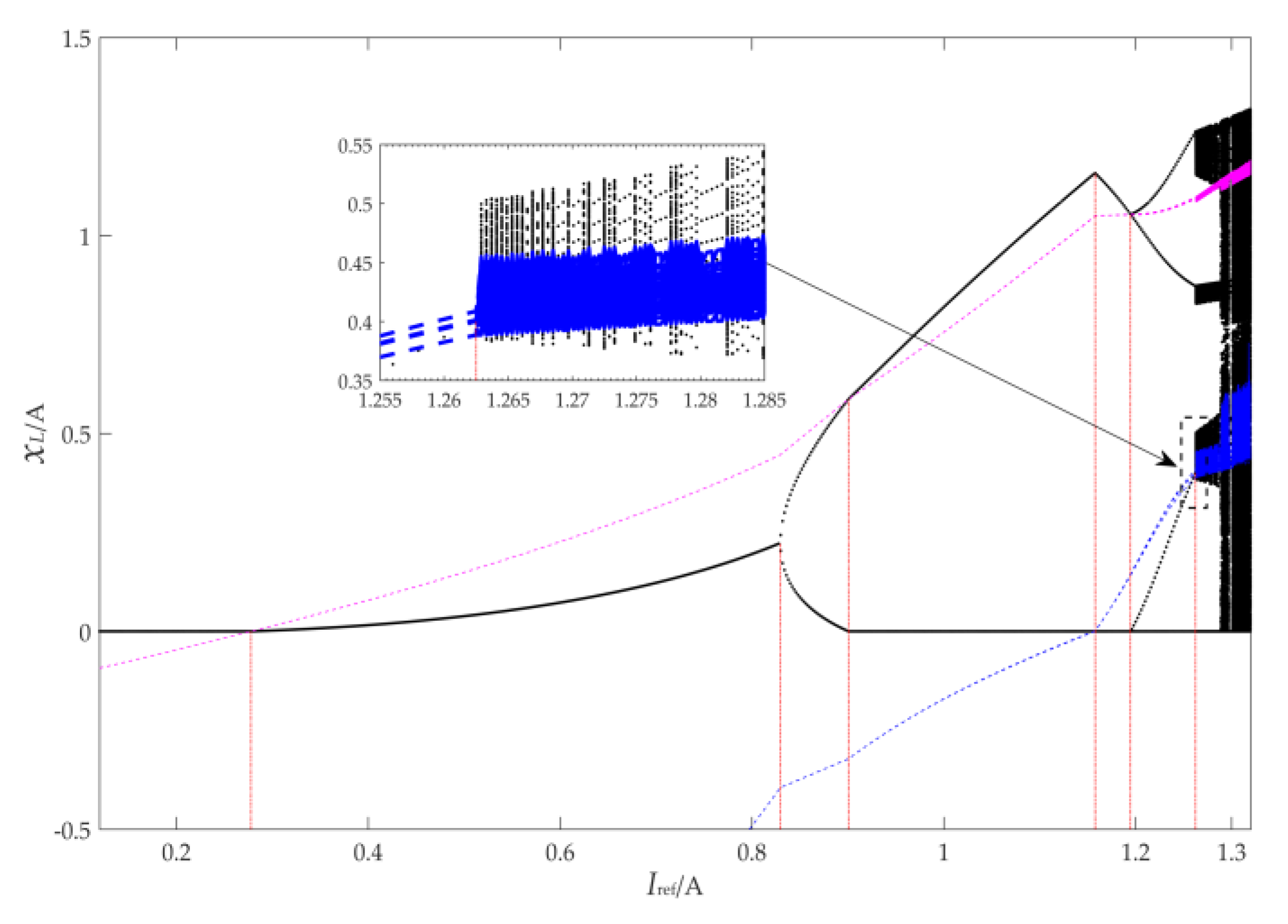
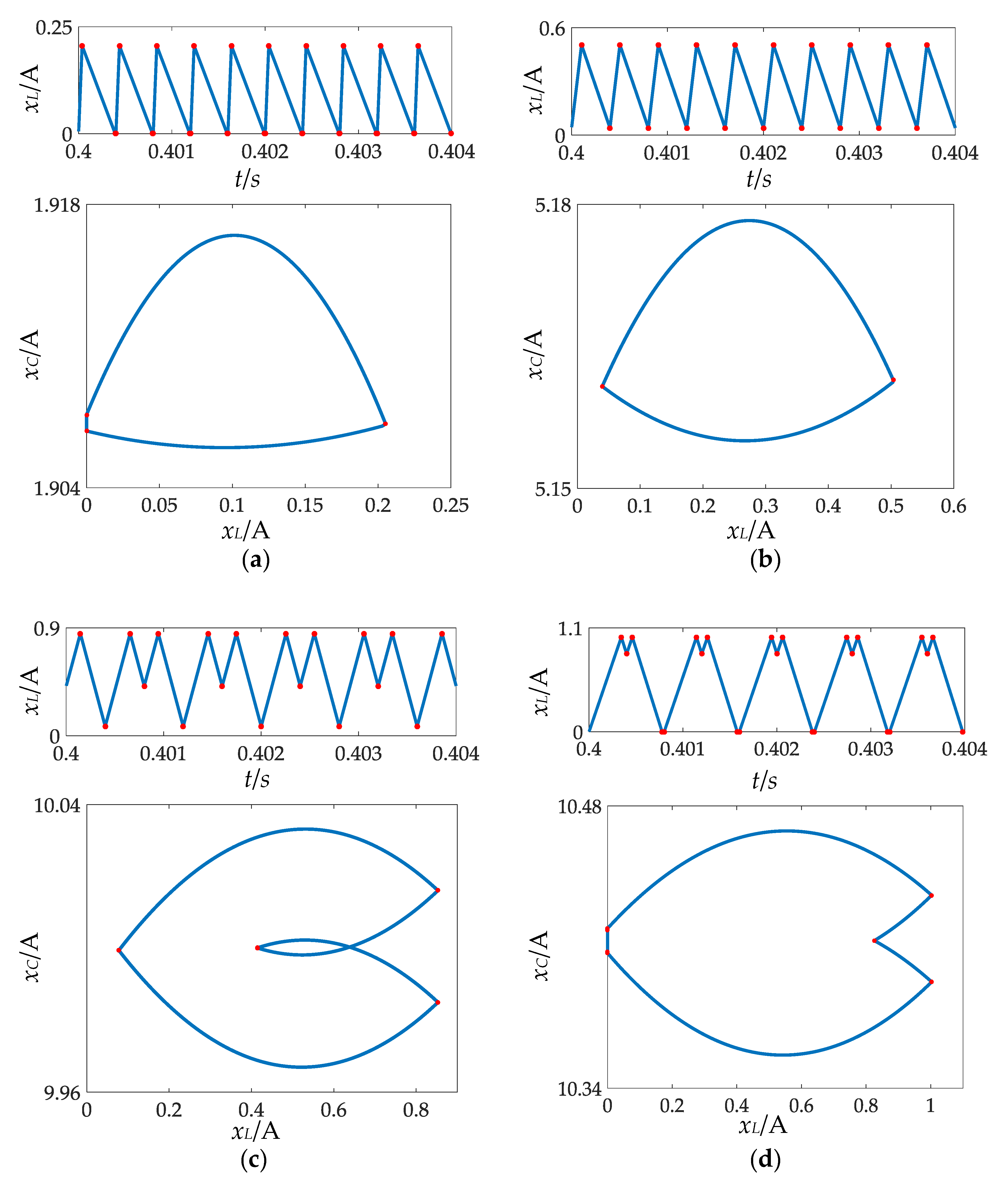
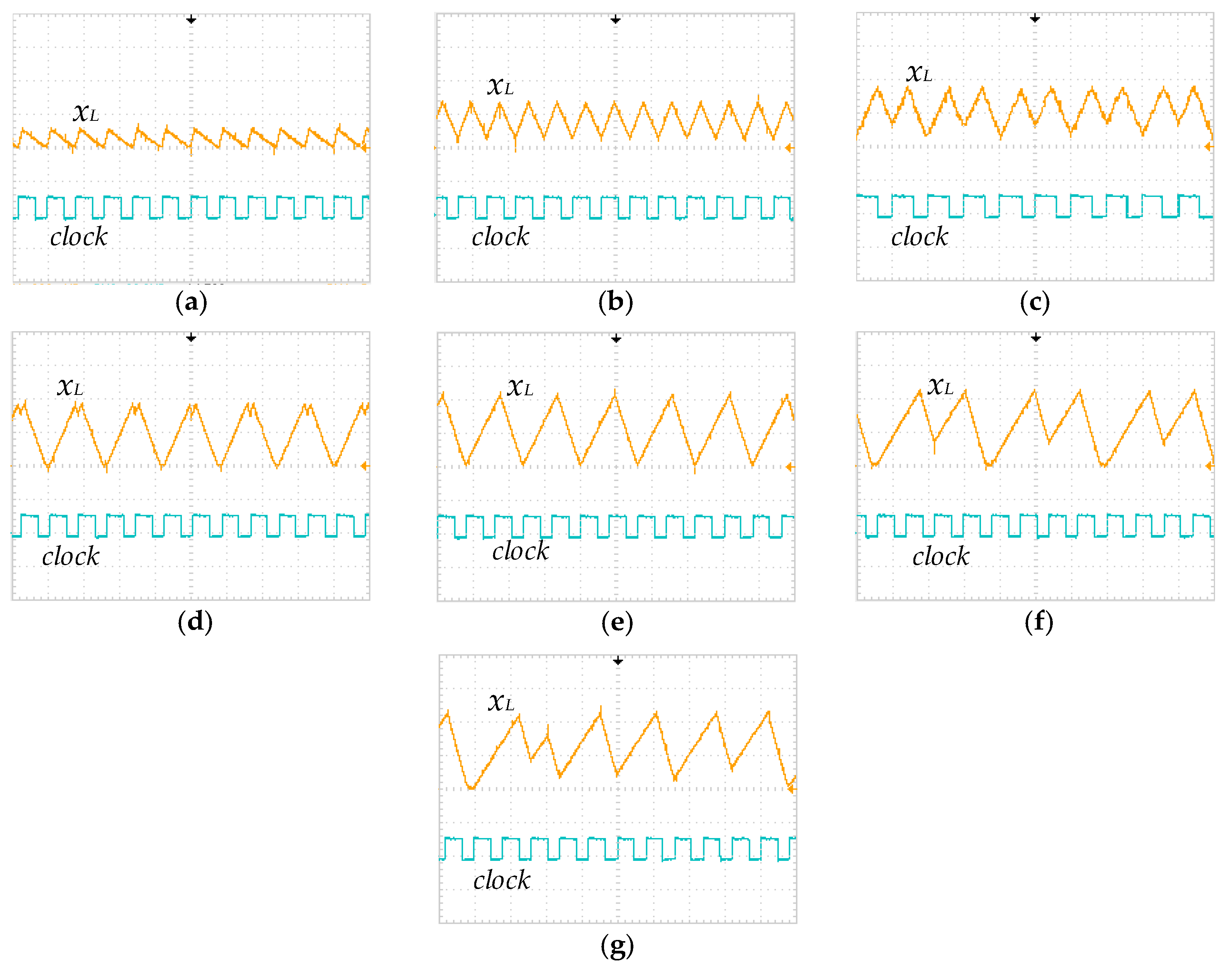
• As I_ref ∈ [0.1200,0.2778], the system works in the F₃ pattern of period-1. In this pattern, there are three modes in each period of the system, which means the system is in the DCM state. Then, the first border collision bifurcation occurs in the system at I_ref = 0.2779 A. Because the inductor current in the steady state collides with Ib₂, the operating mode changes and the working patterns of the converter system change from F₃ to F₂.
• During I_ref ∈[0.2779,0.8295], the system still works in the period-1 state, but the operating mode is F₂. At this time, the system has two modes in each period. When I_ref = 0.8296, the system generates period doubling bifurcation and enters period-2. Since there is no border collision bifurcation, the working patterns are extended to F₂F₂.
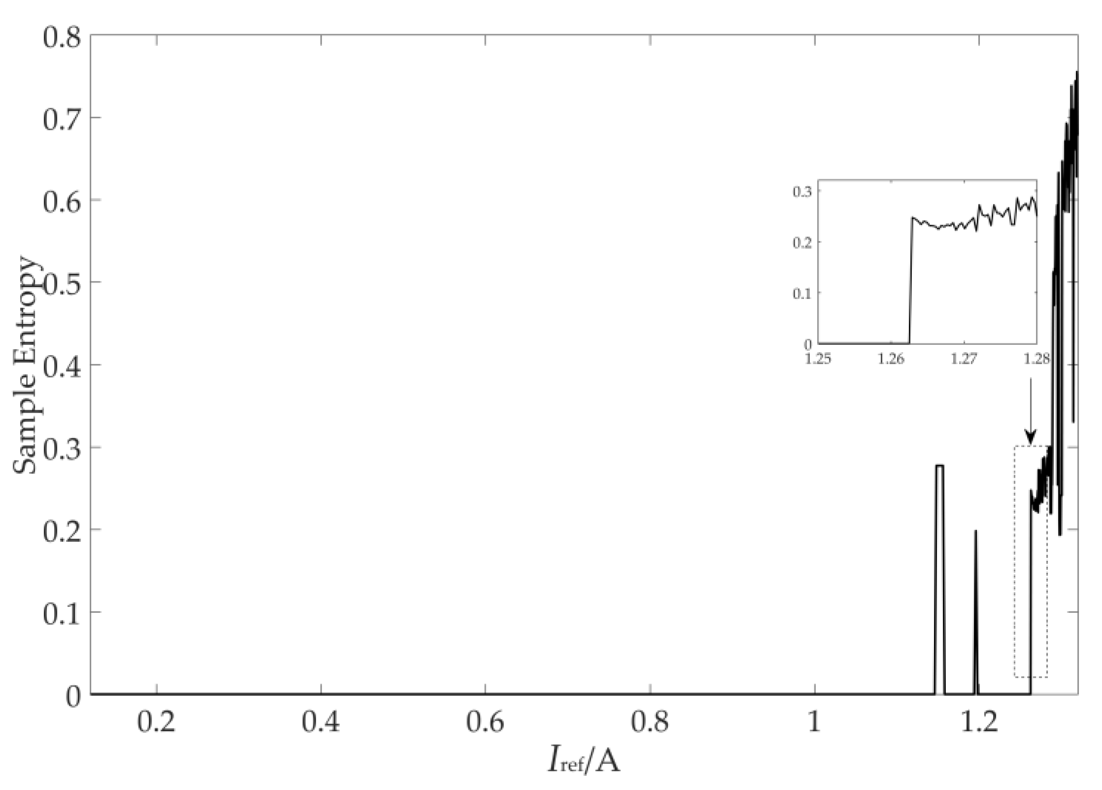
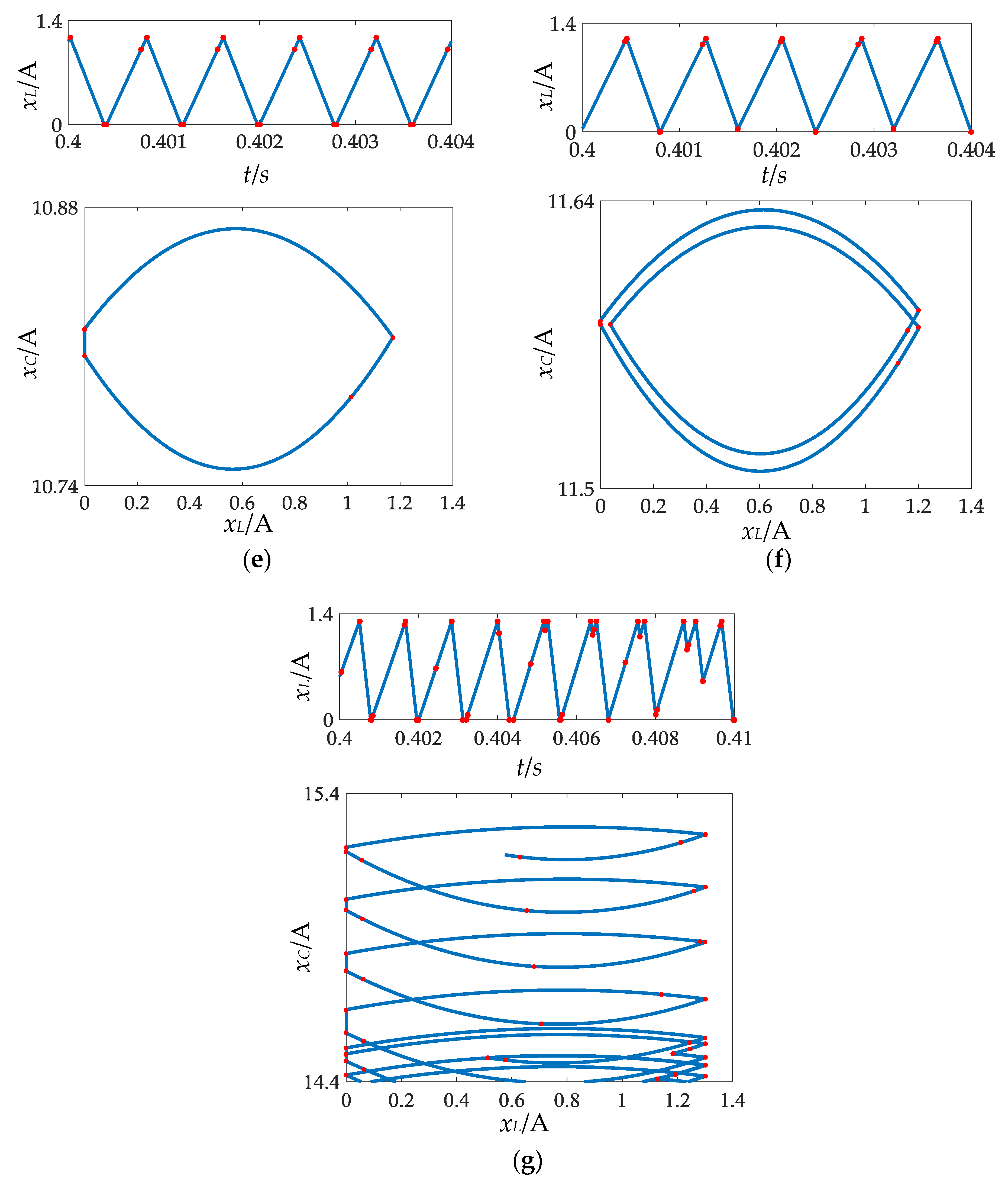
• When I_ref ∈[0.8296,1.1946], the system works in period-2. We found that two bounder collisions of the system occur in this area because the inductance current of the system collides with the borderline of Ib₂ and Ib₁ at I_ref = 0.9007 and I_ref = 1.1578 A, respectively. Hence, the operating pattern of the converter system changes from F₂F₂ at I_ref ∈[0.8296,0.9006] to F₂F₃ at I_ref ∈[0.9007,1.1577] and to F₁F₃ at I_ref ∈[1.1578,1.1946]. From the entropy value of three period-2 orbits shown in Figure 7, the permutation entropy value of period-2 is greater than the corresponding entropy value of any working pattern in the entirety of period-1. The sample entropy, used for assessing the complexity of the time sequence shown in Figure 9, is the negative logarithm of the probability of if two sets of simultaneous data points of length m have a distance smaller than r, then two sets of simultaneous data points of length m + 1 also have a distance smaller than r [28]. However, with the change in sample entropy, we could not find the bifurcation information of the system under period-1 and period-2 states.
• As I_ref ∈[1.1947,1.2624], the system works in the period-4 state with the working pattern F₁F₂F₁F₃, and there are seven modes in this state. Then, the fifth time border collision bifurcation of a fixed point and Ib₁ curve collision occur once more in the system at I_ref = 1.2625 A. At this time, LLE shown in Figure 10 is greater than 0 and the mode switching shows disorder, which means that the system is beginning enter the chaotic state. When I_ref ≥ 1.2625 A, a number of border collisions occur in the chaotic state, as depicted in Figure 7. Then, the value of permutation entropy is no longer stable, exhibiting similar characteristics to the LLE, and its corresponding value is greater than any period. The characteristics described are consistent with Bandt C et al. [20].

Moreover, the fourth border collision bifurcation occurs at I_ref = 1.1947 A. Since the system has unstable characteristic roots at the same time, the system generates period-doubling bifurcation and enters the period-4 state. The working pattern is extended while F₂ switches to F₃.

To further explain permutation entropy, the time-domain simulating waveforms with phase plane, and the experimental results at the typical values of I_ref, are illustrated in Figure 11 and Figure 12, respectively. We found that the values of the permutation entropy correspond to the complexity of the working waveforms. In summary, the presented MSTS-PE can quantify the complexity of the operation states of the buck converter, and the established MSTS can characterize the bifurcation phenomena of the system.

6. Discussion and Conclusions

Phase space reconstruction is a method of reconstructing attractors based on finite data to study the dynamic behavior of a system. Its basic idea is that the evolution of any component in the system is determined by its interactions with other components. In DC-DC converters, the dynamic information of one component is implicit in any related component; that is, the original dynamic system model can be reconstructed with one variable observation in the system.

The quantization process of the sequence information based on the permutation entropy, and comparison between permutation entropy and the traditional symbol sequence method, are described in Section 3. In addition, the permutation entropy and sample entropy of buck converter are shown in Figure 7 and Figure 9. The permutation entropy seems to be a better indicator in some circumstances because it has high robust performance and anti-interference ability for analysis of the mixed signal. Permutation entropy overcomes shortcomings, like the poor relative consistency of sample entropy and time consuming calculation of multi-scale entropy, which is easily affected by the non-stationarity and outliers of time sequences. For a better description of nonlinear dynamic behaviors of a system from a time sequence, MSTS was proposed to describe the dynamic features of a DC-DC converter. In addition, distinguished from joint entropy, permutation entropy combined with MSTS only needs one sequence to identify the system features. This concept is also consistent with the concept of phase space reconstruction.

Based on the theory of phase space reconstruction, the permutation entropy of the DC-DC converter under the determined parameters is obtained by sorting each group of m-dimensional vectors. In this paper, we found that the higher the frequency of mode switching, the more complex the obtained MSTS. This means that the higher the complexity of the corresponding system, the larger the permutation entropy value. With the fluctuation in the permutation entropy value of different control parameters, the nonlinear dynamic behaviors of a DC-DC converter can be better quantified.

References

1. Tse, C.K.; Di Bernardo, M. Complex Behavior in Switching Power Converters. Proc. IEEE 2002, 90. [Google Scholar] [CrossRef]
2. Rodriguez, E.; El Aroudi, A.; Guinjoan, F.; Alarcon, E. A Ripple-Based Design-Oriented Approach for Predicting Fast-Scale Instability in DC-DC Switching Power Supplies. IEEE Trans. Circuit Syst. I Reg. Papers 2012, 59, 215–227. [Google Scholar] [CrossRef]
3. Zhou, S.; Zhou, G.; Wang, Y.; Liu, X.; Xu, S. Bifurcation analysis and operation region estimation of current-mode-controlled SIDO boost converter. IET Power Electron. 2017, 10, 846–853. [Google Scholar] [CrossRef]
4. Fossas, E.; Olivar, G. Study of chaos in the buck converter. IEEE Trans. Circuit Syst. I Fundam. Theory Appl. 1996, 43, 13–25. [Google Scholar] [CrossRef] [Green Version]
5. Li, X.; Tang, C.; Dai, X.; Hu, A.; Nguang, S. Bifurcation Phenomena Studies of a Voltage Controlled Buck-Inverter Cascade System. Energies 2017, 10, 708. [Google Scholar] [CrossRef]
6. Dai, D.; Tse, C.K.; Ma, X. Symbolic analysis of switching systems: Application to bifurcation analysis of DC/DC switching converters. IEEE Trans. Circuit Syst. I Reg. Papers 2005, 52, 1632–1643. [Google Scholar] [CrossRef]
7. Han, M. Prediction Theory and Method of Chaotic Time Series, 1st ed.; China Water Power Press: Beijing, China, 2007; pp. 36–61. ISBN 978-7-5084-4534-2. [Google Scholar]
8. Yan, D.; Wang, W.; Chen, Q. Nonlinear Modeling and Dynamic Analyses of the Hydro–Turbine Governing System in the Load Shedding Transient Regime. Energies 2018, 11, 1244. [Google Scholar] [CrossRef]
9. Iu, H.H.C.; Tse, C.K. A study of synchronization in chaotic autonomous Cuk DC/DC converters. IEEE Trans. Circuit Syst. I: Fundam. Theory Appl. 2000, 47, 913–918. [Google Scholar] [CrossRef] [Green Version]
10. Wang, J.; Wang, Y. Study on the Stability and Entropy Complexity of an Energy-Saving and Emission-Reduction Model with Two Delays. Entropy-Switz. 2016, 18, 371. [Google Scholar] [CrossRef]
11. Khalil, H.K. NONLINEAR SYSTEMS, 2nd ed.; Prentice-Hall, Inc.: New Jersey, NJ, USA, 1996; ISBN 0-13-P8U24-8. [Google Scholar]
12. Wang, X.; Zhang, B.; Qiu, D. The Quantitative Characterization of Symbolic Series of a Boost Converter. IEEE Trans. Power Electron. 2011, 26, 2101–2105. [Google Scholar] [CrossRef]
13. Li, N.; Pan, W.; Xiang, S.; Zhao, Q.; Zhang, L.; Mu, P. Quantifying the Complexity of the Chaotic Intensity of an External-Cavity Semiconductor Laser via Sample Entropy. IEEE J. Quantum Electron. 2014, 50, 1–8. [Google Scholar] [CrossRef]
14. Liu, J.; Xu, H. Nonlinear Dynamic Research of Buck Converter Based on Multiscale Entropy. In Proceedings of the 2015 Fifth International Conference on Instrumentation and Measurement, Computer, Communication and Control, Qinhuangdao, China, 18–20 September 2015. [Google Scholar] [CrossRef]
15. Zhao, M.; Xu, G. Feature extraction of power transformer vibration signals based on empirical wavelet transform and multiscale entropy. IET Sci. Meas. Technol. 2018, 12, 63–71. [Google Scholar] [CrossRef]
16. Xiao, M.; Wei, H.; Xu, Y.; Wu, H.; Sun, C. Combination of R-R Interval and Crest Time in Assessing Complexity Using Multiscale Cross-Approximate Entropy in Normal and Diabetic Subjects. Entropy 2018, 20, 497. [Google Scholar] [CrossRef]
17. Ray, A. Symbolic dynamic analysis of complex systems for anomaly detection. Signal Process. 2004, 84, 1115–1130. [Google Scholar] [CrossRef]
18. Xie, F.; Zhang, B.; Yang, R.; Qiu, D. Quantifying the Complexity of DC-DC Switching Converters by Joint Entropy. IEEE Trans. Circuits Syst. II 2014, 61, 579–583. [Google Scholar] [CrossRef]
19. Zhang, B.; Qu, Y. The Precise Discrete Mapping of Voltage-Fed DCM Boost Converter and Its Bifurcation and Chaos. Trans. China Electrotech. Soc. 2002, 17, 43–47. [Google Scholar] [CrossRef]
20. Bandt, C.; Pompe, B. Permutation entropy: A natural complexity measure for time series. Phys. Rev. Lett. 2002, 88. [Google Scholar] [CrossRef] [PubMed]
21. El-mezyani, T.; Wilson, R.; Sattler, M.; Srivastava, S.K.; Edrington, C.S.; Cartes, D.A. Quantification of complexity of power electronics based systems. IET Electr. Syst. Trans. 2012, 2, 211. [Google Scholar] [CrossRef]
22. Gray, R.M. Entropy and Information Theory, 2nd ed.; Springer Science & Business Media: New York, NY, USA, 2011; ISBN 978-1-4419-7969-8. [Google Scholar]
23. Zunino, L.; Rosso, O.A.; Soriano, M.C. Characterizing the Hyperchaotic Dynamics of a Semiconductor Laser Subject to Optical Feedback Via Permutation Entropy. IEEE J. Select. Topics Quantum Electron. 2011, 17, 1250–1257. [Google Scholar] [CrossRef] [Green Version]
24. Gao, Y.; Villecco, F.; Li, M.; Song, W. Multi-Scale Permutation Entropy Based on Improved LMD and HMM for Rolling Bearing Diagnosis. Entropy 2017, 19, 176. [Google Scholar] [CrossRef]
25. Packard, N.H.; Crutchfield, J.P.; Farmer, J.D.; Shaw, R.S. Geometry from a time series. Phys. Rev. Lett. 1980, 45, 712–716. [Google Scholar] [CrossRef]
26. Stark, J.; Broomhead, D.S.; Davies, M.E.; Huke, J. Takens embedding theorems for forced and stochastic systems. Nonlinear Anal. Theory Methods Appl. 1997, 30, 5303–5314. [Google Scholar] [CrossRef]
27. Zhang, L.; Wang, L. PWM DC—Study on Nonlinear Dynamics Behavior in PWM Switched—Capacitor DC-DC Converter. Acta Electron. Sinica 2008, 36, 266–270. [Google Scholar]
28. Richman, J.S.; Moorman, J.R. Physiological time-series analysis using approximate entropy and sample entropy. Am. J. Physiol. Heart Circ. Physiol. 2000, 278. [Google Scholar] [CrossRef] [PubMed]
Figure 1. Sampling at the mode switching time to build a mode switching time sequence (MSTS).
Energies 11 02747 g001
Figure 2. Procedure to obtain the permutation symbols from the sample period-6 signal as delay time τ = 2.
Energies 11 02747 g002
Figure 3. Generating the K from MSTS as m = 3, τ = 1.
Energies 11 02747 g003
Figure 4. Buck converter with peak current control.
Energies 11 02747 g004
Figure 5. Three modes of a buck converter.
Energies 11 02747 g005
Figure 6. (a) F1 working pattern means that only mode-1 exists in one period; (b) F2 means that mode-1 is performed first in the period, then the switch state changes once and enters into mode-2; and (c) F3 represents the mode in the period change from mode-1 to mode-2 to mode-3.
Energies 11 02747 g006
Figure 7. Permutation entropy of buck converter with Iref as the changing parameter.
Energies 11 02747 g007
Figure 8. Bifurcation diagram of a buck converter with Iref as the changing parameter.
Energies 11 02747 g008
Figure 9. Sample Entropy of buck converter with Iref as the change parameter
Energies 11 02747 g009
Figure 10. Largest Lyapunov exponent (LLE) of a buck converter with Iref as the changing parameter.
Energies 11 02747 g010
Figure 11. Waveforms of inductor current xL and phase plane at (a) Iref = 0.20 A; (b) Iref = 0.50 A; (c) Iref = 0.85 A; (d) Iref = 1.00 A; (e) Iref = 1.17 A; (f) Iref = 1.20 A; and (g) Iref = 1.27 A. In (a) to (g), xC and xL represent the inductor current and capacitor voltage, respectively, and the red marker dot corresponds the mode switching moment.
Energies 11 02747 g011aEnergies 11 02747 g011b
Figure 12. Experimental waveforms of inductor current xL and switching signal at (a) Iref = 0.20 A; (b) Iref = 0.50 A; (c) Iref = 0.85 A; (d) Iref = 1.00 A; (e) Iref = 1.17 A; (f) Iref = 1.20 A; and (g) Iref = 1.27 A.
Energies 11 02747 g012