Energy Management in Buildings with Intermittent and Limited Renewable Resources

Abstract

This work reports a contribution, in a model predictive control multi-agent systems context, introducing a novel integrative methodology to manage energy networks from the demand-side point of view, in the strong presence of intermittent energy sources, including energy storage in households or car batteries. In particular, the article presents a control-based solution for indoor comfort, which, in addition, optimizes the usage of a limited shared energy resource. The control management is applied, in a distributed way, to a set of so-called thermal control areas (TCAs) and demand units, with the objective of minimizing the cost of energy while maintaining the indoor temperature within the comfort zone bounds, and simultaneously not exceeding a limited amount of shared renewable energy. The thermal control areas are, in general, thermodynamically connected, and are also coupled by energy interrelation constraints established in the particular optimization solution. Energy management is performed with a fixed sequential order established from a previously carried out auction, wherein the bids are made by each unit’s demands, acting as demand-side management agents, based on the daily energy price. The developed solution is explained by a basic algorithm that has been applied to different scenarios, and the results have been compared so as to illustrate the benefits and flexibility of the proposed approach, showing less energy consumption and a 37% cost saving.

1. Introduction

Data from the literature [1] shows that 39% of the United States’ primary energy is consumed by buildings, with space heating and cooling being responsible for 54% of the site energy consumption in the residential sector, and 37% in the commercial sector during 2017. In Europe, air conditioning equipment systems are also the main energy consumer in buildings, consisting of 70% of the final energy use [2,3]. Considering these data, the importance of reducing the energy used in all types of building in order to improve their efficiency and sustainability is clear. This theme is nowadays a hot topic for financial, social, and environmental impacts all over the world. Demand response (DR) mechanisms [4,5], are nowadays seen as a reliable option when they are applied to buildings, and they have been able to significantly reduce the energy consumption. DR is nowadays mostly used to encourage customers to manage their daily loads wisely, by considering the electricity price. But even so, DR strategies must be improved in the following two aspects: they need to consider different load types and also need to deal with the distributed renewable resource aspects. In order to provide a response to the novel challenges that DR requires, industries are developing new communication technologies in order to ensure the necessary requirements allowing for effective residential appliance scheduling programs [6,7]. These DR mechanisms, along with demand-side management (DSM) approaches, aim to be a solution in order to support buildings in upcoming smart grids (SG) [8,9], preparing them to work efficiently in an unpredictable environment, where the electrical energy will mainly be provided by intermittent renewable sources [10]. Nowadays, the production of electricity system follows the load. However, the renewable sources of electricity are essentially intermittent, and it is vital that they provide flexibility to the grid so as to absorb the variations from these sources. With SGs, the production is able to control the energy consumption; so, when the sun and wind are available, a building’s consumption needs must be readjusted. In this way, consumers will no longer be mere spectators and will have an active role in the electricity grid system [11]. Distinct approaches are being studied in order to deal with the poor controllability, intermittence, unpredictability and flexibility of renewable green sources, in order to achieve a DSM solution for balancing supply–demand. Additionally, the novel solutions that incorporate the occupants’ behavior inside the buildings, taking into account their energy consumption habits, are evolving. [12]. It has been noted that this is a complex problem, because DSM strategies must consider the control issues of different appliances, such as heating ventilation and air conditioning (HVAC) systems, washing machines, refrigerators, lighting, or even electric vehicle charging.

The study presented in this paper applies to the SG technological environment [13,14], and is intended to provide a response to the renewable resources’ variability, assuming that home appliances will be fully manageable and controllable. These different DSM methods [15] will provide solutions to manage loads in order to achieve a supply–demand balance, such as load control techniques [16,17], which may also involve price signals with distinct tariff prices throughout the day to promote the load shifting [18], as well as other methods that encourage energy conservation, sustainability, and efficiency [19]. Consequently, an original control solution with DSM is proposed based on model-based predictive control (MPC) techniques. In comparison with the other traditional HVAC control solutions used in the residential sector, MPC is capable of saving between 16–41% energy [20]. Therefore, the MPC’s characteristics make it appropriate for load management and optimization processes regarding set-point temperature control [21,22], and [23] for a complete review on MPCs in HVAC control systems.

The MPC control techniques can be applied to problems with a distributed nature [24,25,26,27]. Distributed model predictive control (DMPC) algorithms support distributed sensing and control using local controllers. These controllers can be understood as cooperative agents that decide their actions by considering the information exchanged between them [28]. This is the reason it was the chosen methodology used to tackle the distributed problem presented in this paper. As mentioned, DMPC is appropriate for work in distributed scenarios, and consequently, in multi agent system (MAS) structures, where distinct agents using MPC control strategies are able to interact between them, exchanging information about their state, being impacted by the influences from each other, and using that data to solve/optimize their local control problems [29,30]. In the literature, an agent is defined as an autonomous, pro-active, and social entity, which drives its actions and decisions in order to accomplish is objective, cooperating/competing by considering the external influences created by its pairs [31]. The SG idea was built around this concept; an infrastructure where different identities cooperate so as to acquire a collective perception. The developed system presented in this paper considers the existence of autonomous agents, which are entities defined as thermal control areas (TCAs). The entities are within a distributed framework, where the TCAs cooperate in a coordinated way by exchanging information in order to achieve a global goal [32,33,34]. The TCAs’ demand units share green resources between themselves, and each minimizes its energy costs according to a given cost function. In this paper, global coordination is achieved using a sequential access order, which is established by a proposed green energy auction mechanism. The global objective is to maximize green energy consumption.

The work presented here is distinct and has the advantage of providing a solution that integrates a set of features and concepts that are already present in smart grid technologies, such as intelligent control, distributed generation, energy efficiency, energy saving, DSM, intermittent energy resources, smart loads management, thermal comfort, real-time price negotiation, and energy auction markets mechanisms. These characteristics deliver a unique structure, where different subsystems with different roles can be intelligently combined, aiming for a more efficient, secure, and sustainable energy system. Therefore, this work intends to provide an innovative DMPC solution that is able to efficiently manage networks, adapting consumption to the smart grid using intermittent renewable energy sources.

In particular, it provides new developments in DSM using renewable energy sources, and uses a backup of fossil energy, using an hourly auction access mechanism that allows for managing loads in order to balance the demand and supply. Equally, the proposed DSM energy usage optimization scheme allows the consumer to choose a trade-off between comfort or energy savings, in an hourly manner. The energy forecast inclusion (renewable and fossil fuel) enables the system to decide how and when to split the energy among the users, while at the same time satisfying all of the power and comfort constraints. It has been noticed that this innovative distributed optimization scheme is also suitable for use in scenarios where energy sources, renewable or fossil, are scarce, and energy must be rationed or carefully spent. For instance, in remote areas or on cruise ships where the rooms must be acclimatized and the fuel resources are limited. The organization of this paper is as follows: Section 2 describes the proposed approach, the global concept scenario, and the dynamical formulation. Section 3 designates the DMPC formulation and implemented algorithm. Section 4 illustrates the methodology used with simulation results. In Section 5, the key conclusions are drawn and future objectives are suggested.

2. Distributed Scenario Set-Up

The conceptual scenario involves a set of buildings with electrical power provided by a renewable energy grid with a local energy storage capability. Henceforward, the term “house” will be applied so as to classify any type of construction for housing, offices, services, or other kinds of analogous buildings.

The set $W=\{w_1,w_2,\dots ,w_{N_S}\}$ identifies the group of houses in consideration, and the different spaces or rooms in each house are specified by N_S sets, given by $D_i=\{d_{i1},d_{i2},\dots ,d_{iN{d}_i}\}$, where $i=1,\dots ,N_S$, and Nd_i is the number of rooms for house i.

Because of the room diversity that can exist in each house, each area may vary in its construction materials, sun exposure, occupancy, and indoor temperature set-points. This variety implies that considerably different energy is needed to weatherize different spaces as well as different fixed consumption profiles.

In this paper, a TCA is an autonomous thermal control entity in an environment where several may coexist in different spaces belonging to houses, seen as an agent in a distributed scenario, where the actions and reactions are treated as a unit on a global distributed environment set, defined by W. Therefore, depending on the infrastructure that is intended to be implemented and to manage, a set of buildings or a simple division may represent a TCA.

The main idea is using a DMPC control law to manage the indoor temperature and energy consumption in each TCA within W. And by doing so, taking advantage of the MPC predictive capabilities and constraint handling, so that each agent can receive this information from the others, as well as about outdoor temperature forecasts, future occupation, indoor temperature frame, and the thermal disturbances profile. Consequently, each agent’s control action depends on its own thermal comfort specifications, and it also depends on its neighbors, the weather forecast, and shared available energy. Feasibility is achieved by using soft constraints in the optimization problem formulation; feasibility is also important for ensuring stability.

This scenario considers the existence of two resources, the red, from the grid provided by the fossil source, and the green, from the renewable or clean source. The first is always available in auction with a kWh price that is always higher than the second. On the contrary, the green is limited, intermittent, and must be consumed, stored, or grid delivered, and when it becomes insufficient, the fossil fuel is consumed and increases the energy costs.

It is assumed here that the traded electricity comes from a wholesale market that is priced in real time, where the market operators (MO) provide the green resource auction. The agents set their bid prices a day-ahead, indicating how much they are willing to pay in order to consume the clean energy. The bid can be made hourly or daily, according to specific consumption needs. If the user knows in advance that they will have a determined period (a day) with a major load profile (due to household appliances, comfort needs, etc.), they will consequently bid higher so as to try to “ensure” green energy (at lower price than red energy). Then, the MO receives the TCA bid value and establishes a sequential order by which the TCA can access green energy. The access order is stored in a matrix, A_O, with a $(N_S\times N)$ dimension. So, each agent comprises a specific TCA, a DMPC controller, and an hourly bid mechanism that provides the DSM. The red resource consumption will have a penalty because of the soft constraint violation imposed by the maximum available green resource. Each TCA sends information on about how much of the clean resource is still available, and when the divisions thermally interact, they also pass information about future temperatures on to one another.

Therefore, in a setup that prioritizes clean energy consumption, the DSM approach allows for managing the distributed loads in order to obtain a supply–demand balance, providing indoor thermal comfort that allows for lesser costs, consequently reducing CO₂ emissions. With this active DSM control strategy, the energy supplied from the intermittent resources is maximized by the optimal control used for the various appliances.

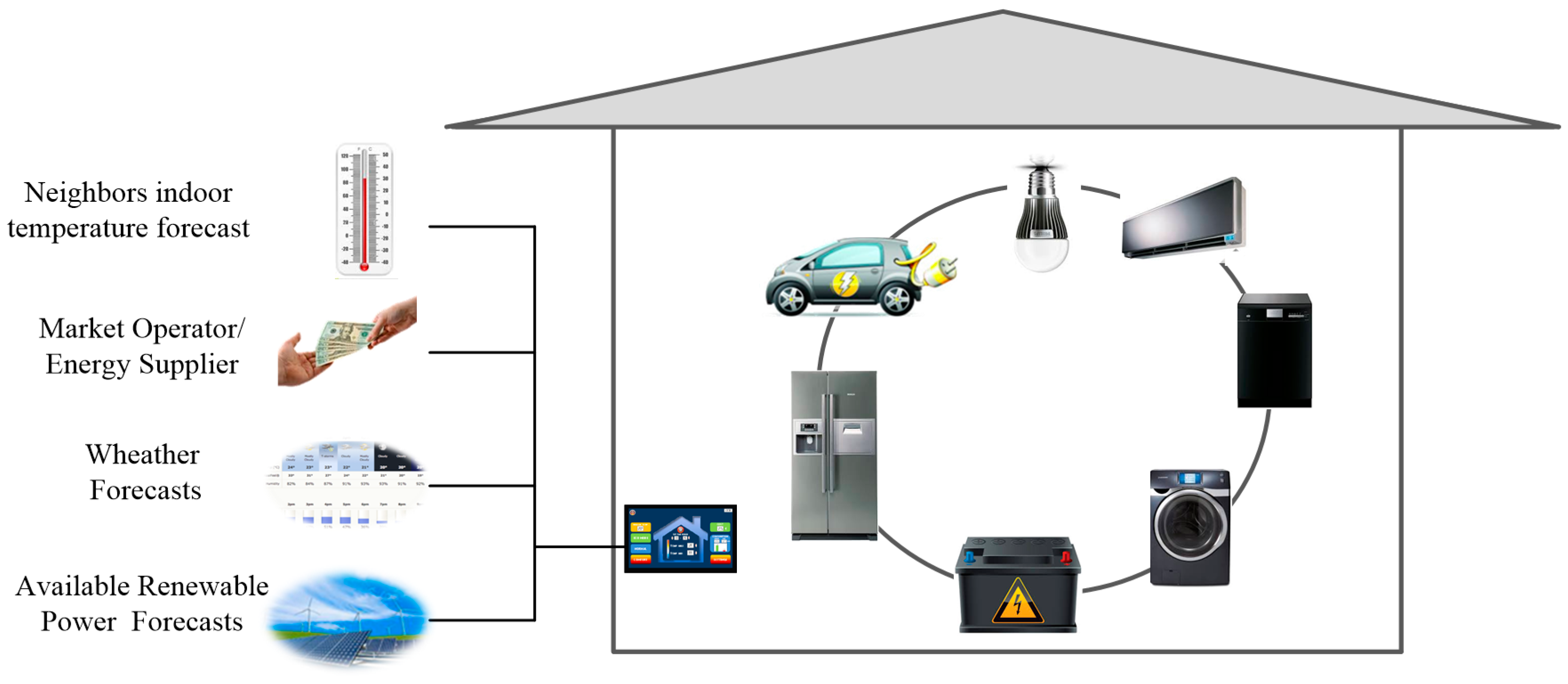
Each TCA has several external inputs, namely, the outdoor temperature; the available renewable power forecasts; the MO kWh price, the access order to the renewable resource; and, when dynamically coupled, the neighbors’ indoor temperature forecasts. It has been noticed that the indoor temperature is the only private information that is exchanged, and each agent is blind to the others’ dynamics and inputs. However, this issue may not be relevant when the adjacent areas belong to the same building, but it may represent a barrier when the adjacent areas are from distinct agents. Figure 1 presents an example of the implemented TCA framework.

The example depicted in Figure 1 shows that the implemented system is dependent on weather and power forecasts. As wind and solar power are not dispatched, their production levels need to be predictable. For wind power, the 24 h ahead of the prediction averages the absolute error and can be between 10–20% of the installed capacity for one single zone. When the aggregation of zones is made, the value may drop to 5–8% [35,36]. The forecast error is significantly lowered for the first six hours. The solar energy forecast has similar problems as that of the wind. Nevertheless, in order for the sun’s path through the sky to be known, solar power forecasting needs a higher predictability. Also, nowadays, temperature forecasts are particularly reliable and accurate, with more than a 92% accuracy for one day ahead forecasting [37].

TCA Dynamical Models

House models can be built with more or less complexity, depending of what aim is to be accomplished. As described in the literature [38], a first order energy balance model is used to describe a basic room or division, considering only the existing dominant dynamics. Consider the dynamic model of each TCA:

$$\frac{d{T}_l^i}{dt}=\frac{1}{C_{l_{eq}}^i}\left(Q_{l_{heat}}^i-Q_{l_{losses}}^i+Q_{l_{Pd}}^i\right),$$

(1)

$$Q_{l_{losses}}^i=\frac{T_{oa}-T_l^i}{R_{l_{eq}}^i}+{\displaystyle \sum }_{\begin{array}{l}g=1\\ \left(g\ne l\right)\end{array}}^{N{d}_i}\frac{T_g^i-T_l^i}{R_{l{g}_{eq}}^i{C}_{l_{eq}}^i}\Delta t+{\displaystyle \sum }_{\begin{array}{l}h=1\\ \left(h\ne i\right)\end{array}}^{Ns}{\displaystyle \sum }_{m=1}^{N{d}_h}\frac{T_m^h-T_l^i}{R_{l{m}_{eq}}^{ih}{C}_{l_{eq}}^i},$$

(2)

$$R_{l_{eq}}^i={\left(\frac{1}{R_{l_{roof}}^i}+\frac{1}{R_{l_{windows}}^i}+\frac{1}{R_{l_{walls}}^i}+\frac{1}{R_{l_{th}}^i}\right)}^{-1},$$

(3)

where, in Equation (1), $Q_{l_{losses}}^i$ is the heat and cooling losses (kW) from the TCA (i) division (l), $T_l^i$ is the inside temperature (°C), $C_{l_{eq}}^i$ is the equivalent thermal capacitance (kJ/°C), $Q_{l_{heat}}^i$ is the heat and cooling power (kW) and $Q_{l_{Pd}}^i$ is the thermal disturbances (kW) (e.g., the load generated by the occupants, direct sunlight, electrical devices, or doors and windows’ opening, in order to recycle the indoor air). In Equations (2) and (3), $T_{oa}$ is the outdoor temperature (°C), $R_{l{g}_{eq}}^i$ is the thermal resistance between division (l) and the adjacent zone (g), $R_{l_{eq}}^i$ is the parallel equivalent thermal resistance (°C/kW), $R_{l_{th}}^i$ is the air thermal resistance to the bulk of division, and $R_{l{m}_{eq}}^{ih}$ is the thermal resistance between division (l) and the adjacent zone (m) from subsystems (i) and (h). Note that these are the basic equations for structure thermal modelling and can be explained by the several divisions and floors interacting between them.

Equation (1) can be written, for the N_s TCAs and for each division (l), in the following format:

$$T_l^i\left(k+1\right)=A_{ll}^{ii}{T}_l^i\left(k\right)+B_l^i{u}_l^i\left(k\right)+\underset{\begin{array}{c}thermalcontributions\\ fromadjacentareas\\ insidethesamehouse\end{array}}{\underbrace{{\displaystyle \sum }_{\begin{array}{l}g=1\\ \left(g\ne l\right)\end{array}}^{N{d}_i}\left(A_{lg}^{ii}{T}_l^i\left(k\right)\right)}}+\underset{\begin{array}{c}thermalcontributions\\ fromadjacentareas\\ fromotherhouses\end{array}}{\underbrace{{\displaystyle \sum }_{\begin{array}{l}h=1\\ \left(h\ne i\right)\end{array}}^{Ns}{\displaystyle \sum }_{p=1}^{N{d}_h}\left(A_{lm}^{ih}{T}_m^h\left(k\right)\right)}}+v_l^i\left(k\right),$$

(4)

$$\begin{array}{l}{A}_{ll}^{ii}=\left(1-\frac{\Delta t}{R_{l_{eq}}^i{C}_{l_{eq}}^i}\right),B_l^i=\frac{\Delta t}{C_{l_{eq}}^i},A_{lg}^{ii}={\displaystyle {\displaystyle \sum }_{\begin{array}{l}g=1\\ \left(g\ne l\right)\end{array}}^{N{d}_i}}\frac{T_g^i-T_l^i}{R_{l{g}_{eq}}^i{C}_{l_{eq}}^i}\Delta t,A_{lm}^{ih}={\displaystyle {\displaystyle \sum }_{\begin{array}{l}h=1\\ \left(h\ne i\right)\end{array}}^{Ns}}{\displaystyle {\displaystyle \sum }_{m=1}^{N{d}_h}}\frac{T_m^h-T_l^i}{R_{l{m}_{eq}}^{ih}{C}_{l_{eq}}^i}\Delta t,\\ v_l^i=\frac{P_{l_{Pd}}^i\Delta t}{C_{l_{eq}}^i}+\frac{T_{oa}\Delta t}{R_{l_{eq}}^i{C}_{l_{eq}}^i}.\end{array}$$

(5)

where N_s is number of TCA’s, Nd_i is the number of divisions inside the subsystem (i); $T_l^i$ is the indoor temperature in TCA (i) inside the division (l); $u_l^i$ is the used power to provide comfort in TCA (i) inside the division (l); $A_{lm}^{ih}$ is an element from the state matrix A, which relates to the state (indoor temperature) in the division (m) from TCA (h), with the state from division (l) in TCA (i); $v_l^i$ is the thermal disturbance in the TCA/subsystem (i) inside the division (l); T_oa is the temperature of the outside air (°C); and $P_{l_{Pd}}^i$ is the thermal disturbance due to the heat produced by the occupants, sunlight, electrical appliances, or any other generic heat sources.

As mentioned, there are several degrees of complexity for house modelling techniques [39]. In this work, more complex or non-linear models would unnecessarily increase the computational time, and also, if the prediction horizon is too long, the computation and the reliability of the optimizer might be a problem. Thus, the model that has been considered is linear and is suitable for control purposes, as follows:

$$x\left(k+1\right)=Ax\left(k\right)+Bu\left(k\right)+v\left(k\right),$$

(6)

where x ∈ ℝⁿ is the state variable, indoor room temperatures, vector containing all of the division temperatures (°C) of all of the TCAs; u ∈ ℝ^m is the input vector containing all of the heating and cooling power sources (W) needed to weatherize each division; v ∈ ℝⁿ includes all of the heat disturbances (W); k is an integer number that denotes discrete time; and A ∈ ℝ^n×n and B ∈ ℝ^n×m are matrices. 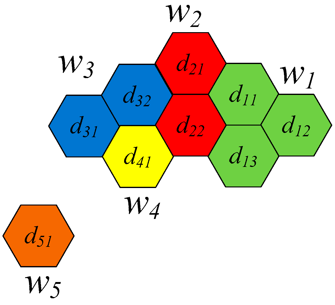Notice that the number of stated variables is n = ${\displaystyle \sum }_{i=1}^{Ns}N{d}_i.$ Thus, as an example of a TCA scenario model, Figure 2 depicts a set of houses/TCAs with different plans and different zones that are thermally connected in a distributed environment. As previously mentioned, side-by-side rooms can be doubly coupled, both thermally and by the power constraint.

For each division, using Equation (4), it can be written in terms of the space-state model, as follows:

$$x_1^1\left(k+1\right)=A_{11}^{11}{x}_1^1\left(k\right)+A_{12}^{11}{x}_2^1\left(k\right)+A_{13}^{11}{x}_3^1\left(k\right)+A_{11}^{12}{x}_1^2\left(k\right)+A_{12}^{12}{x}_2^2\left(k\right)+B_1^1{u}_1^1\left(k\right)+v_1^1\left(k\right)$$

$$x_2^1\left(k+1\right)=A_{22}^{11}{x}_2^1\left(k\right)+A_{21}^{11}{x}_1^1\left(k\right)+A_{23}^{11}{x}_3^1\left(k\right)+B_2^1{u}_2^1\left(k\right)+v_2^1\left(k\right)$$

$$x_3^1\left(k+1\right)=A_{33}^{11}{x}_3^1\left(k\right)+A_{32}^{11}{x}_2^1\left(k\right)+A_{31}^{11}{x}_1^1\left(k\right)+A_{32}^{12}{x}_2^2\left(k\right)+B_3^1{u}_3^1\left(k\right)+v\left(k\right)$$

$$x_1^2\left(k+1\right)=A_{11}^{22}{x}_1^2\left(k\right)+A_{12}^{22}{x}_2^2\left(k\right)+A_{11}^{21}{x}_1^1\left(k\right)+B_1^2{u}_1^2\left(k\right)+v_1^2\left(k\right)$$

$$\begin{gathered} x_2^2\left(k+1\right)=A_{22}^{22}{x}_2^2\left(k\right)+A_{21}^{22}{x}_1^2\left(k\right)+A_{21}^{21}{x}_1^1\left(k\right)+ \\ {A}_{23}^{21}{x}_3^1\left(k\right)+A_{22}^{23}{x}_2^3\left(k\right)+A_{21}^{24}{x}_1^4\left(k\right)+B_2^2{u}_2^2\left(k\right)+v_2^2 \end{gathered}$$

(7)

$$x_1^3\left(k+1\right)=A_{11}^{33}{x}_1^3\left(k\right)+A_{12}^{33}{x}_2^3\left(k\right)+A_{11}^{34}{x}_1^4\left(k\right)+B_1^3{u}_1^3\left(k\right)+v_1^3\left(k\right)$$

$$x_2^3\left(k+1\right)=A_{22}^{33}{x}_2^3\left(k\right)+A_{21}^{33}{x}_1^3\left(k\right)+A_{21}^{34}{x}_1^4\left(k\right)A_{21}^{32}{x}_1^2\left(k\right)+A_{22}^{32}{x}_2^2\left(k\right)+B_2^3{u}_2^3\left(k\right)+v_2^3\left(k\right)$$

$$x_1^4\left(k+1\right)=A_{11}^{44}{x}_1^4\left(k\right)+A_{11}^{43}{x}_1^3\left(k\right)+A_{12}^{43}{x}_2^3\left(k\right)A_{12}^{42}{x}_2^2\left(k\right)+B_1^4{u}_1^4\left(k\right)+v_1^4\left(k\right)$$

$$x_1^5\left(k+1\right)=A_{11}^{55}{x}_1^5\left(k\right)+B_1^5{u}_1^5\left(k\right)+v\left(k\right)$$

resulting in the following:

$$\begin{array}{c}\left[\begin{array}{c}{x}_1^1\left(k+1\right)\\ x_2^1\left(k+1\right)\\ x_3^1\left(k+1\right)\\ x_1^2\left(k+1\right)\\ x_2^2\left(k+1\right)\\ x_1^3\left(k+1\right)\\ x_2^3\left(k+1\right)\\ x_1^4\left(k+1\right)\\ x_1^5\left(k+1\right)\end{array}\right]=\left[\begin{array}{ccccccccc}{A}_{11}^{11}& A_{12}^{11}& A_{13}^{11}& A_{11}^{12}& A_{12}^{12}& 0& 0& 0& 0\\ A_{21}^{11}& A_{22}^{11}& A_{23}^{11}& 0& 0& 0& 0& 0& 0\\ A_{31}^{11}& A_{31}^{11}& A_{33}^{11}& A_{32}^{12}& 0& 0& 0& 0& 0\\ A_{11}^{21}& 0& 0& A_{11}^{22}& A_{12}^{22}& 0& 0& 0& 0\\ A_{21}^{21}& 0& A_{23}^{21}& A_{21}^{21}& A_{22}^{22}& 0& A_{22}^{23}& A_{21}^{24}& 0\\ 0& 0& 0& 0& 0& A_{11}^{33}& A_{12}^{33}& A_{11}^{34}& 0\\ 0& 0& 0& A_{21}^{32}& A_{22}^{32}& A_{21}^{33}& A_{22}^{33}& A_{21}^{34}& 0\\ 0& 0& 0& A_{12}^{42}& 0& A_{11}^{43}& A_{12}^{43}& A_{11}^{44}& 0\\ 0& 0& 0& 0& 0& 0& 0& 0& A_{11}^{55}\end{array}\right]\left[\begin{array}{c}{x}_1^1\left(k\right)\\ x_2^1\left(k\right)\\ x_3^1\left(k\right)\\ x_1^2\left(k\right)\\ x_2^2\left(k\right)\\ x_1^3\left(k\right)\\ x_2^3\left(k\right)\\ x_1^4\left(k\right)\\ x_1^5\left(k\right)\end{array}\right]+\hfill \\ +\left[\begin{array}{lllllllll}{B}_1^1& 0& 0& 0& 0& 0& 0& 0& 0\\ 0& B_2^1& 0& 0& 0& 0& 0& 0& 0\\ 0& 0& B_3^1& 0& 0& 0& 0& 0& 0\\ 0& 0& 0& B_1^2& 0& 0& 0& 0& 0\\ 0& 0& 0& 0& B_2^2& 0& 0& 0& 0\\ 0& 0& 0& 0& 0& B_1^3& 0& 0& 0\\ 0& 0& 0& 0& 0& 0& B_2^3& 0& 0\\ 0& 0& 0& 0& 0& 0& 0& B_1^4& 0\\ 0& 0& 0& 0& 0& 0& 0& 0& B_1^5\end{array}\right]\left[\begin{array}{c}{u}_1^1\left(k\right)\\ u_2^1\left(k\right)\\ u_3^1\left(k\right)\\ u_1^2\left(k\right)\\ u_2^2\left(k\right)\\ u_1^3\left(k\right)\\ u_2^3\left(k\right)\\ u_1^4\left(k\right)\\ u_1^5\left(k\right)\end{array}\right]+\left[\begin{array}{c}{v}_1^1\left(k\right)\\ v_2^1\left(k\right)\\ v_3^1\left(k\right)\\ v_1^2\left(k\right)\\ v_2^2\left(k\right)\\ v_1^3\left(k\right)\\ v_2^3\left(k\right)\\ v_1^4\left(k\right)\\ v_1^5\left(k\right)\end{array}\right].\hfill \end{array}$$

3. MPC Formalization

For large-scale systems, the centralized MPC is considered practically unfeasible, because of the limitations imposed by the computational efforts and by communication, and the scientific community is consensual about overcoming these drawbacks using distributed MPC optimization algorithms in multi-agent setups [25]. Smart grids are characterized by complex dynamics and mutual influences between all of the involved identities, and the DMPC algorithms should be able to deal with the different types of existent coupling among the subsystems; the constraints’ satisfaction must also be safeguarded in the closed-loop system, as well as the required stability and feasibility, see the literature [26] for a comprehensive survey. Stability issues will not be treated here, but feedback stability is provided by choosing a sufficiently long predictive horizon and is verified by results presented in Section 4.

The DMPC methodologies are generally characterized by the type of couplings or by the interactions assumed between the involved variables or subsystems [40,41,42]. The scenario presented here represents the most complex example; the subsystems are doubly coupled, dynamically and by the power constraints.

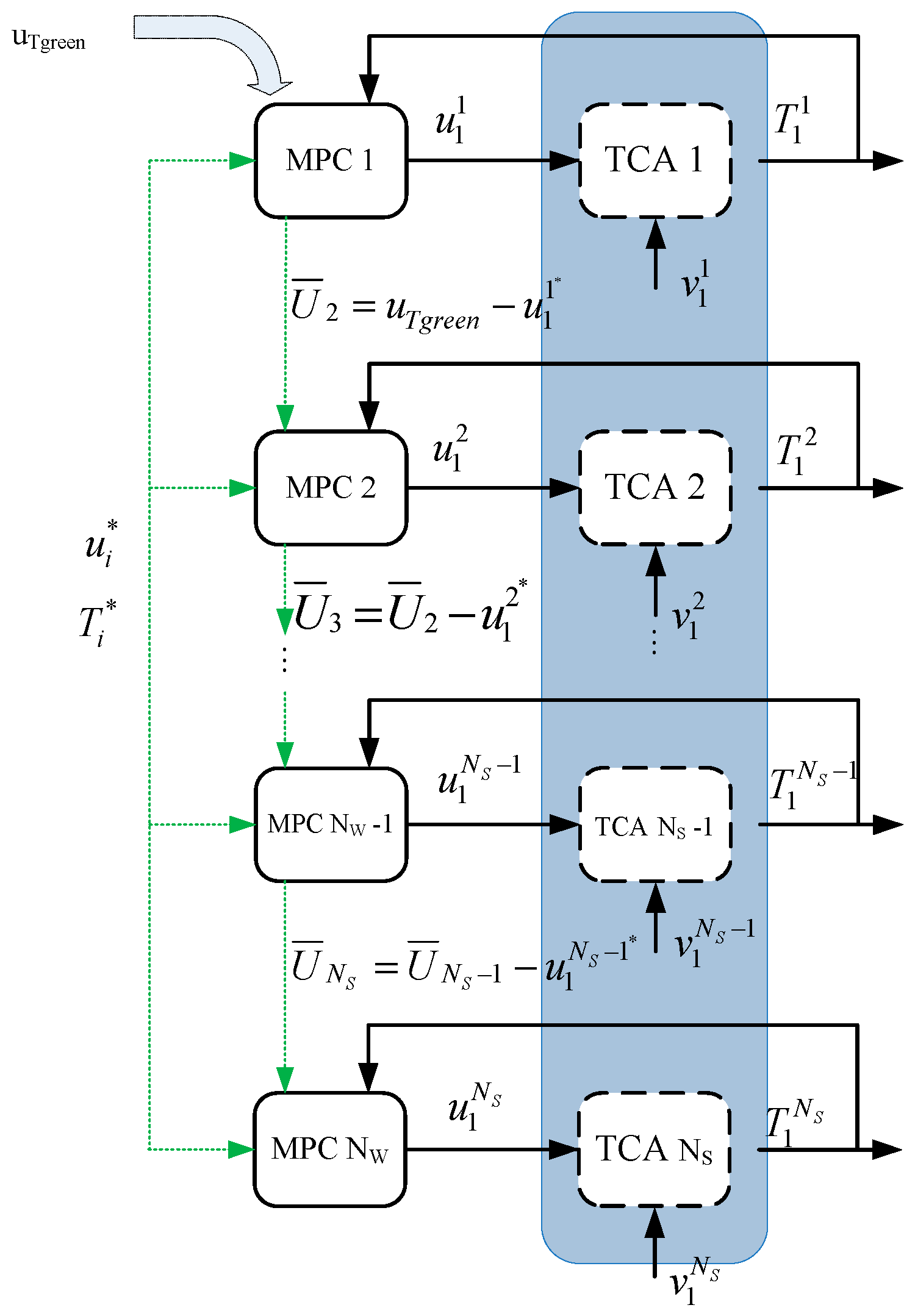
Figure 3 depicts the sequential scheme proposed for the DMPC solution. Note that each TCA updates their data, and the available power is passed sequentially, one by one, guaranteeing the satisfaction of the green resource constraints. The MPC optimization is solved by each TCA at each time step, according to the sequential DMPC (the scheme depicted in Figure 3), which considers N_W TCA. The available green power forecast is received by the agent who made the highest bid (first in the sequential access scheme) and this information is used as the power constraint value in Equation (9). The agent optimization problem predicts the consumption, subtracts it from the maximum availability that was initially received, and passes that information on to the next on the sequence in the list.

In Figure 3, $u_{Tgreen}$ represents the green resource forecasts, ${\overline{U}}_i$ is the maximum available expected green resource for TCA (i), $T_l^i$ and ${T_l^i}^{\ast }$ are the indoor temperature and indoor temperature prediction, $u_l^i$ and ${u_l^i}^{\ast }$ are the optimal power generated by the MPC controller and the predicted consumption, and $v_l^i$ represents the thermal disturbances. The maximum available resource, ${\overline{U}}_i$, is different for each TCA, and takes into account which TCAs are ahead in the access order consumed, as follows:

$${\overline{U}}_i=u_{Tgreen}-{\displaystyle \sum }_{l=1}^{i-1}{U}_l.$$

(8)

The minimization problem is a trade-off between four terms, energy consumption to weatherize the space, the power peak and the constraints violations related to the comfort temperature frame and the limited green power. In the literature [23], the control action is typically conditioned only by the consumption and temperature. The combination of these four terms forms the cost function that is able to deal with the intermittent energy resource. The formulated optimization is a distributed linear constrained quadratic programing optimization problem, which is coupled by constraints that must be solved sequentially for each TCA at each time step. The typically distributed MPC relies on the quadratic cost functions, and in principle, a linear cost function could be used. Furthermore, a quadratic cost function provides smoother signals for the actuators, because the square functions penalize smaller errors than the linear relations, so it is expected that the quadratic cost provides smoother energy profiles with less saturation signals for the actuators. Constrained quadratic programming can be solved using, for instance, a MATLAB^® fmincon routine. Accordingly, the optimization problem in each TCA is given by Equations (9) and (16)–(19), as follows:

$$\begin{array}{l}\underset{U,\overline{\epsilon },\underset{\_}{\epsilon },\overline{\gamma },\underset{\_}{\gamma }}{min}{J}_i\left(k\right)={\displaystyle {\displaystyle \sum }_{j=0}^{H_p-1}}\left[{\displaystyle {\displaystyle \sum }_{l=1}^{N{d}_i}}\underset{Consumption}{\underbrace{u_l^i{(k+j)}^T{\phi }_l^i{u}_l^i\left(k+j\right)}}\right]+{\displaystyle {\displaystyle \sum }_{l=1}^{N{d}_i}}\underset{Powerpeaks}{\underbrace{{\varphi }_{i}max\left\{{u_l^i}^2\left(k\right),\dots ,{u_l^i}^2\left(k+H_p-1\right)\right\}}}\\ +{\displaystyle {\displaystyle \sum }_{j=1}^{H_p}}\left[{\displaystyle {\displaystyle \sum }_{l=1}^{N{d}_i}}\left(\underset{Comfortviolation}{\underbrace{{\epsilon }_l^i{(k+j)}^T{\Xi }_l^i{\epsilon }_l^i(k+j}})+\underset{Powerviolation}{\underbrace{{\gamma }_l^i{(k+j)}^T{\Psi }_l^i{\gamma }_l^i\left(k+j\right)}}\right)\right]\end{array}$$

(9)

$$\begin{array}{cc}\hfill \underset{U_i,{\epsilon }_i,{\gamma }_i}{min}{J}_i\left(k\right)& ={\epsilon }_i^T\left(k\right){\Xi }_i{\epsilon }_i\left(k\right)+{\gamma }_i^T\left(k\right){\Psi }_i{\gamma }_i\left(k\right)+U_i^T\left(k\right)R_i{U}_i\left(k\right)\hfill \\ & +{\displaystyle {\displaystyle \sum }_{l=1}^{N{d}_i}}{\varphi }_{i}max\left\{{u_l^i}^2\left(k\right),\dots ,{u_l^i}^2\left(k+H_p-1\right)\right\}\hfill \end{array}$$

(10)

With the following:

$$U_i\left(k\right)=\left[\begin{array}{l}{U}_i^1\left(k\right)\\ U_i^2\left(k\right)\\ ⋮\\ U_i^{Nd}\left(k\right)\end{array}\right],$$

(11)

$${\epsilon }_i\left(k\right)=\left[\begin{array}{l}{\overline{\epsilon }}_i^1\left(k\right)\\ {\overline{\epsilon }}_i^2\left(k\right)\\ ⋮\\ {\overline{\epsilon }}_i^{Nd}\left(k\right)\\ {\underset{\_}{\epsilon }}_i^1\left(k\right)\\ {\underset{\_}{\epsilon }}_i^2\left(k\right)\\ ⋮\\ {\underset{\_}{\epsilon }}_i^{Nd}\left(k\right)\end{array}\right],{\overline{\epsilon }}_i^l\left(k\right)=\left[\begin{array}{l}{\overline{\epsilon }}_i^l\left(k+1\right)\\ {\overline{\epsilon }}_i^l\left(k+2\right)\\ ⋮\\ {\overline{\epsilon }}_i^l\left(k+H_P\right)\end{array}\right],{\underset{\_}{\epsilon }}_i^l\left(k\right)=\left[\begin{array}{l}{\underset{\_}{\epsilon }}_i^l\left(k+1\right)\\ {\underset{\_}{\epsilon }}_i^l\left(k+2\right)\\ ⋮\\ {\underset{\_}{\epsilon }}_i^l\left(k+H_P\right)\end{array}\right],$$

(12)

$${\gamma }_i\left(k\right)=\left[\begin{array}{l}{\overline{\gamma }}_i\left(k\right)\\ {\underset{\_}{\gamma }}_i\left(k\right)\end{array}\right],{\overline{\gamma }}_i\left(k\right)=\left[\begin{array}{l}{\overline{\gamma }}_i\left(k+1\right)\\ {\overline{\gamma }}_i\left(k+2\right)\\ ⋮\\ {\overline{\gamma }}_i\left(k+H_P\right)\end{array}\right]\mathrm{and}{\underset{\_}{\gamma }}_i\left(k\right)=\left[\begin{array}{l}{\underset{\_}{\gamma }}_i\left(k+1\right)\\ {\underset{\_}{\gamma }}_i\left(k+2\right)\\ ⋮\\ {\underset{\_}{\gamma }}_i\left(k+H_P\right)\end{array}\right].$$

(13)

In compact form, Equation (9) results in a quadratic optimization problem, namely:

$$\underset{Z_i}{min}{J}_i\left(k\right)=Z_i^T\Theta Z_i+{\displaystyle \sum }_{l=1}^{N{d}_i}{\varphi }_{il}max\left\{{u_l^i}^2\left(k\right),\dots ,{u_l^i}^2\left(k+H_p-1\right)\right\}$$

(14)

With the following:

$$Z_i=\left[\begin{array}{l}{U}_i\\ {\epsilon }_i\\ {\gamma }_i\end{array}\right],\Theta =\left[\begin{array}{lll}{\phi }_i& 0& 0\\ 0& {\Xi }_i& 0\\ 0& 0& {\Psi }_i\end{array}\right]$$

(15)

and is subject to the following constraints:

$$\begin{array}{cc}\hfill x_l^i\left(k+j+1\right)=& A_{ll}^{ii}{x}_l^i\left(k+j\right)+B_l^i{u}_l^i\left(k+j\right)+\underset{\begin{array}{c}predictedtemperatures\\ fromadjacentareas\\ insidethesamehouse\end{array}}{\underbrace{{\displaystyle \sum _{\begin{array}{l}g=1\\ \left(g\ne l\right)\end{array}}^{N{d}_i}}\left(A_{lg}^{ii}{\tilde{x}}_l^i\left(k+j\right)\right)}}\hfill \\ & \begin{array}{c}\hfill +\underset{\begin{array}{c}predictedtemperatures\\ fromadjacentareas\\ fromotherhouses\end{array}}{\underbrace{{\displaystyle \sum _{\begin{array}{l}h=1\\ \left(h\ne i\right)\end{array}}^{Ns}}{\displaystyle \sum _{m=1}^{N{d}_h}}\left(A_{lm}^{ih}{\tilde{x}}_m^h\left(k+j\right)\right)}}+v_l^i\left(k+j\right)\\ \hfill (j=1\dots H_P)\end{array}\hfill \end{array}$$

(16)

$${\underset{\_}{T}}_l^i\left(k+j\right)-{\underset{\_}{\epsilon }}_l^i\left(k+j\right)\le x_l^i\left(k+j\right)\le {\overline{T}}_l^i\left(k+j\right)+{\overline{\epsilon }}_l^i\left(k+j\right)$$

(17)

$${\underset{\_}{U}}_i\left(k+j-1\right)-{\underset{\_}{\gamma }}_i\left(k+j-1\right)\le {\displaystyle \sum }_{l=1}^{N{d}_i}{u}_l^i\left(k+j-1\right)\le {\overline{U}}_i\left(k+j-1\right)+{\overline{\gamma }}_i\left(k+j-1\right)$$

(18)

$${\underset{\_}{\gamma }}_i,{\overline{\gamma }}_i,{\underset{\_}{\epsilon }}_l^i,{\overline{\epsilon }}_l^i\ge 0.$$

(19)

In Equation (9), $u_l^i$ is the power control input (the space is cooled when $u_l^i$ < 0 and is heated when $u_l^i$ > 0) of house (i) and room (l). $N{d}_i$ represents the number of rooms inside the house (i), ${\Psi }_{\mathrm{i}}$ represents the penalty value when the power constraint is exceeded, ${\varphi }_i$ is the penalty value for the peak power, ${\Xi }_i$ is the penalty value when the comfort range is overcome, and H_P is the prediction horizon. In Equation (17), ${\underset{\_}{T}}_l^i$ and ${\overline{T}}_l^i$ are the established max–min comfort temperature boundaries and ${\overline{\epsilon }}_l^i$ and ${\underset{\_}{\epsilon }}_l^i$ represent the temperature violation vectors. In Equation (18), ${\overline{\gamma }}_i$ and ${\underset{\_}{\gamma }}_i$ represent the power violations, and ${\overline{U}}_i$, and ${\underset{\_}{U}}_{\mathrm{i}}$ (with ${\underset{\_}{U}}_i=-{\overline{U}}_i$) are the maximum green available resources left to TCA (i). We have noted that in each TCA (i), the power consumed in all divisions may not exceed ${\overline{U}}_i$. In Equation (16), $x_l^{i^{\ast }}$ and $u_l^{i^{\ast }}$ represent the predicted temperature and power consumption within the prediction horizon, respectively.

The weighting coefficients in the cost function penalize the different terms between them, giving more importance to some relative to others. Also, as we are using soft constraints, the comfort and power constraints can always be exceeded, although, when the ratio between the coefficients is higher than 104, the controller ensures comfort by satisfying the temperature constraint or power constraint completely, respectively. With this structure, each TCA may vary the penalty values hourly, increasing the flexibility of all of the systems. The user is able to parameterize different time frames during the day, allowing for the choice between cost savings or comfort.

Algorithm

In this subsection, the DMPC optimization algorithm is presented. The algorithm code was written in MATLAB^®, using the optimization routine (fmincon) in order to find the optimal power sequence for each house (Equation (14)), subject to the constraints (Equations (16)–(19)). The agents set their bid prices a day-ahead, indicating how much they are willing to pay in order to consume clean energy. Then, the MO receives the TCAs’ bid value and establishes a sequential order by which the TCAs can access green energy. The access order is stored in a matrix, A_O. The minimization problem is solved using the first TCA, which, after knowing how much will be consumed, sends the information about how much of clean resource is still available to the next. The minimization problem is solved for each TCA in the sequential scheme, presented in Figure 3. The algorithm’s main steps are summarized in Algorithm 1.

Algorithm 1. Distributed model predictive control (DMPC) algorithm—the implemented sequential scheme.

Required for all TCAs: Thermal disturbances, comfort temperature gap, hourly constraints parameters, and hourly auction bid.

for k = 1:N do

Apply to all TCA $u_l^i\left(1\right)$ from k − 1 instant to obtain $T_l^i\left(k\right)$

Apply to all TCA ${u_l^i}^{\ast }\left(1:N\right)$ from k − 1 instant to obtain ${u_l^i}^{\ast }\left(k:k+N-1\right)$ predictions

Communicate temperature predictions to adjacent TCAs

Set sequence order at k instant to green resource based on the bid values

for i = 1:NS (number of TCAs) do

Verify TCA’s reference in matrix AO

Obtain optimal sequence $u_l^i\left(1:N\right)$ solving Equation (9), $J_i\left(k\right)$

Update available green resource values for next TCA in matrix AO

end for

Update batteries available energy

end for

4. Results

In order to explain and prove this concept, one-day simulation results were obtained from three houses, as follows: two of them were side-by-side, and consequently, were thermally interacting (with a thermal resistance of the walls between them of R₁₂ = 30 °C/kW), and the third was isolated. It has been noted that the houses’ controllers need to inform each other about future temperatures when their houses are thermally interconnected. In this case, consider the brown and two blues zones (notice that the blue zones interact through a wall) in Figure 2, as an example of what was simulated.

Table 1. Distributed parameters.

Parameter	TCA 1	TCA 2	TCA 3	Units
Req	50	50	75	°C/kW
Ceq	9.2 × 103	9.2 × 103	9.2 × 103	kJ/°C
Green Price (per kWh)	0.09	0.08	0.07	€
Red Price (per kWh)	0.18			€

The red price is the fixed kWh cost from the grid, and the green price is the bid value (kWh price) that each thermal control area (TCA) is willing to pay.

presents the TCAs’ thermal characteristics and the bid value (made in a previous auction, provided by the MO) that establishes the access order. The used prediction horizon value, H_P, for all of the simulations is 24 h. The performance of the controllers is measured using the closed-loop total energy consumption, as shown in Equations (20)–(23), as follows:

$$J^u={\displaystyle \sum }_{k=0}^{H_p-1}\left|u\left(k\right)\right|\Delta t,$$

(20)

the peak power consumption is as follows:

$$J^p=max\{\left|u\left(0\right)\right|,\dots ,\left|u\left(H_p-1\right)\right|\},$$

(21)

the total comfort violation is as follows:

$$J^{\epsilon }={\displaystyle \sum }_{k=0}^{H_p}\left(\left|\overline{\epsilon }\left(k\right)\right|+\left|\underset{\_}{\epsilon }\left(k\right)\right|\right)\Delta t,$$

(22)

and the total power violation is as follows:

$$J^{\gamma }={\displaystyle \sum }_{k=0}^{H_p}\left(\left|\overline{\gamma }\left(k\right)\right|+\left|\underset{\_}{\gamma }\left(k\right)\right|\right)\Delta t.$$

(23)

The performance index summarizes the controller behavior and allows comparing distinct parameterization and quickly evaluating if the consumer preferred energy savings or comfort.

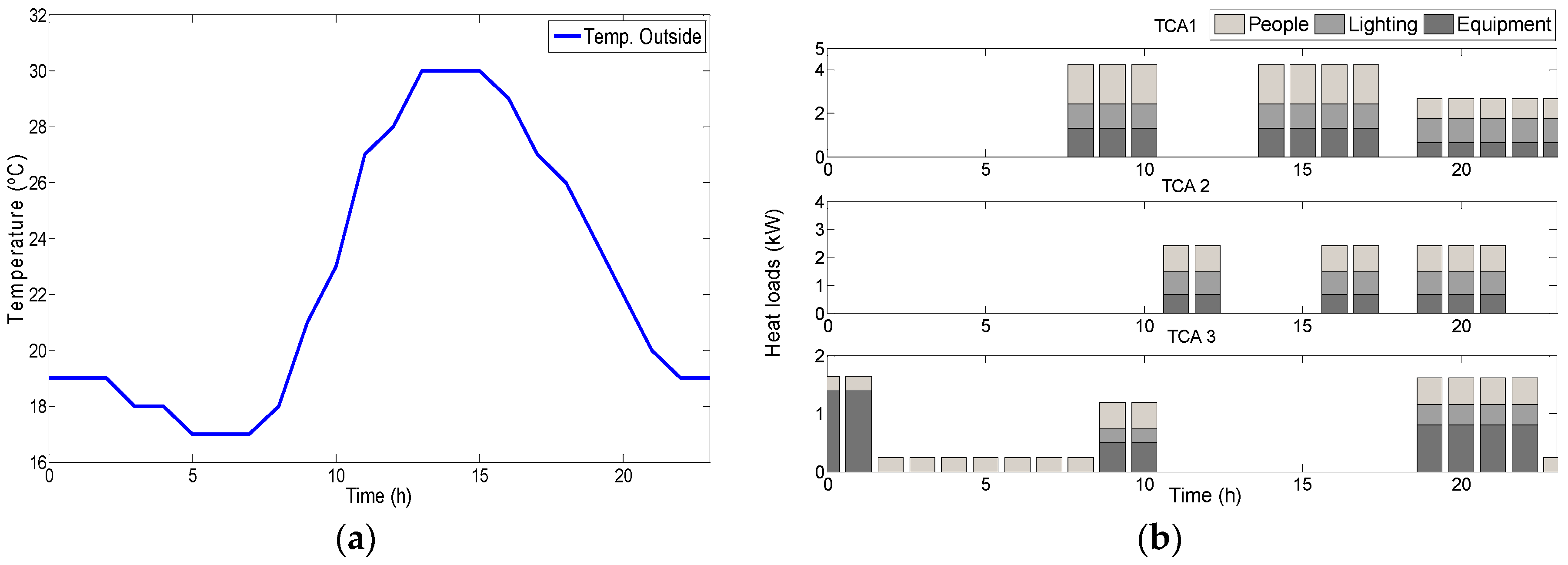
In order to simplify the sequence order, we considered TCA 1, TCA 2, and TCA 3 during the 24 h period. However, despite this simplification, which was intended for a better understanding of the proposed solution, the built system also supported differentiated hourly access orders. The outdoor ambient temperature profile (Figure 4a) was measured on 3 June 2016 from a sensor located at the authors’ affiliation in Lisbon, Instituto Superior de Engenharia de Lisboa (ISEL) [43], Building F. The TCA 1 and TCA 2 load profile, presented in Figure 4b, correspond to two adjacent classrooms in building F, with computers and monitors prepared for 12 and 6 students, respectively. The classrooms are available between 08:00 to 23:00 (night classes), and the occupancy varies according the class schedules. The TCA 3 load profile corresponds to a room in the student’s dormitory (building R), with three students. The loads between 11:00 and 19:00 are considered as nothing or as negligible, and between 21:00 and 01:00, the equipment heat loads are mainly related to cooking, the dishwasher, and the washing and drying of clothes.

The thermal disturbances were obtained considering the hourly contributions of the occupants, lighting, and appliance gains to the peak and latent loads, according American Society of Heating, Refrigerating and Air-Conditioning Engineers (ASHRAE) [44].

The thermal characteristics and prices for all of the agents and scenarios are presented in Table 1.

The developed system considers that each TCA is independent from the others, and that they may have different hourly penalty values favoring cost or temperature. Thus, in order to explain this concept, distinct scenarios are presented. The first, is considered a balanced scenario, with no energy storage and no explicit preference between comfort and consumption.

Table 2. Penalty values scenarios I and II.

Parameter	A1	A2	A3
Comfort penalty—$\Xi$	50	50	50
Power penalty—ψ	100	100	30
Peak power penalty—$\varphi$	2	2	2
Consumption penalty—φ	1	1	1

shows the penalty values that are used in Scenarios I and II.

Figure 5, Figure 6 and Figure 7 depict the obtained results.

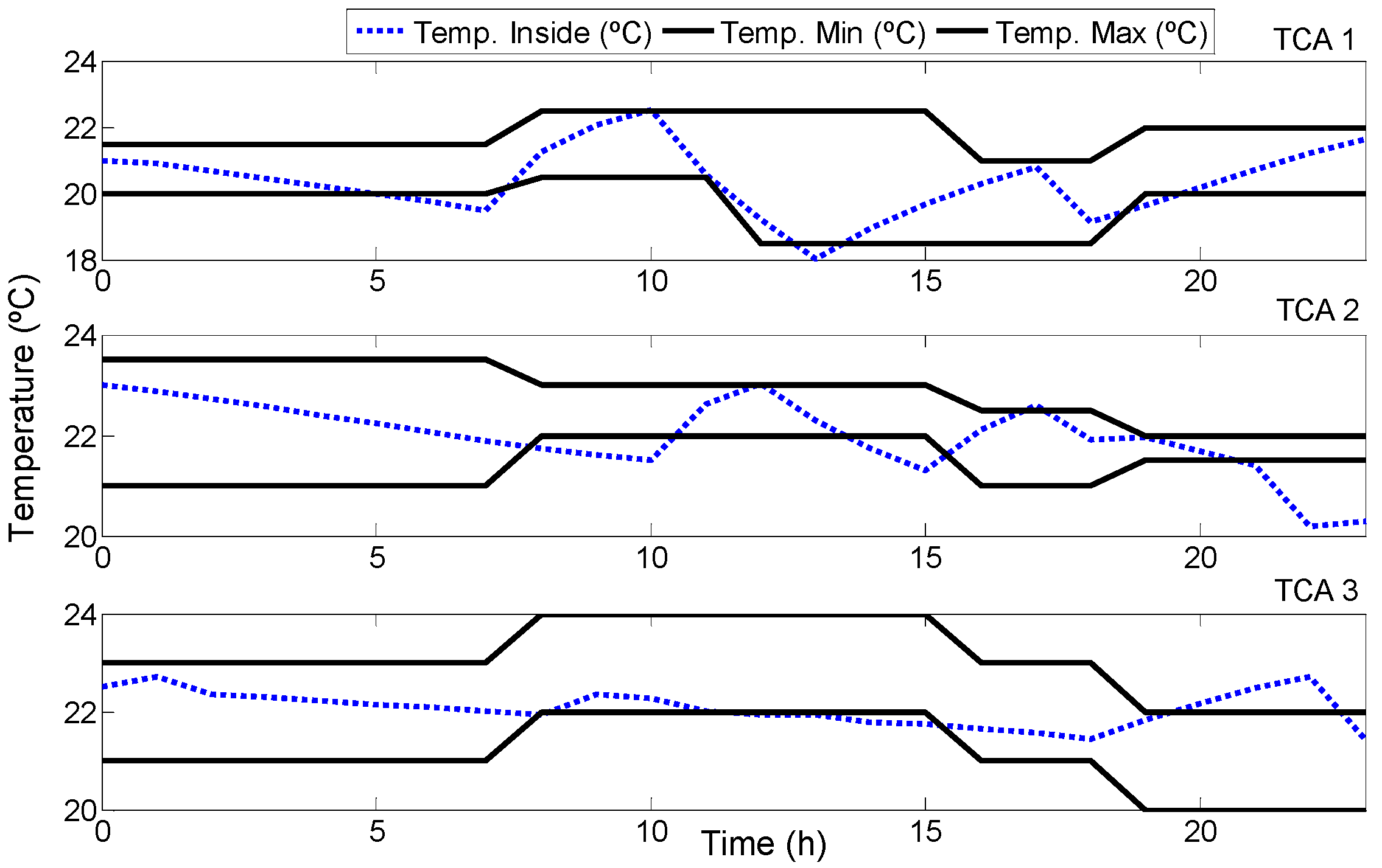
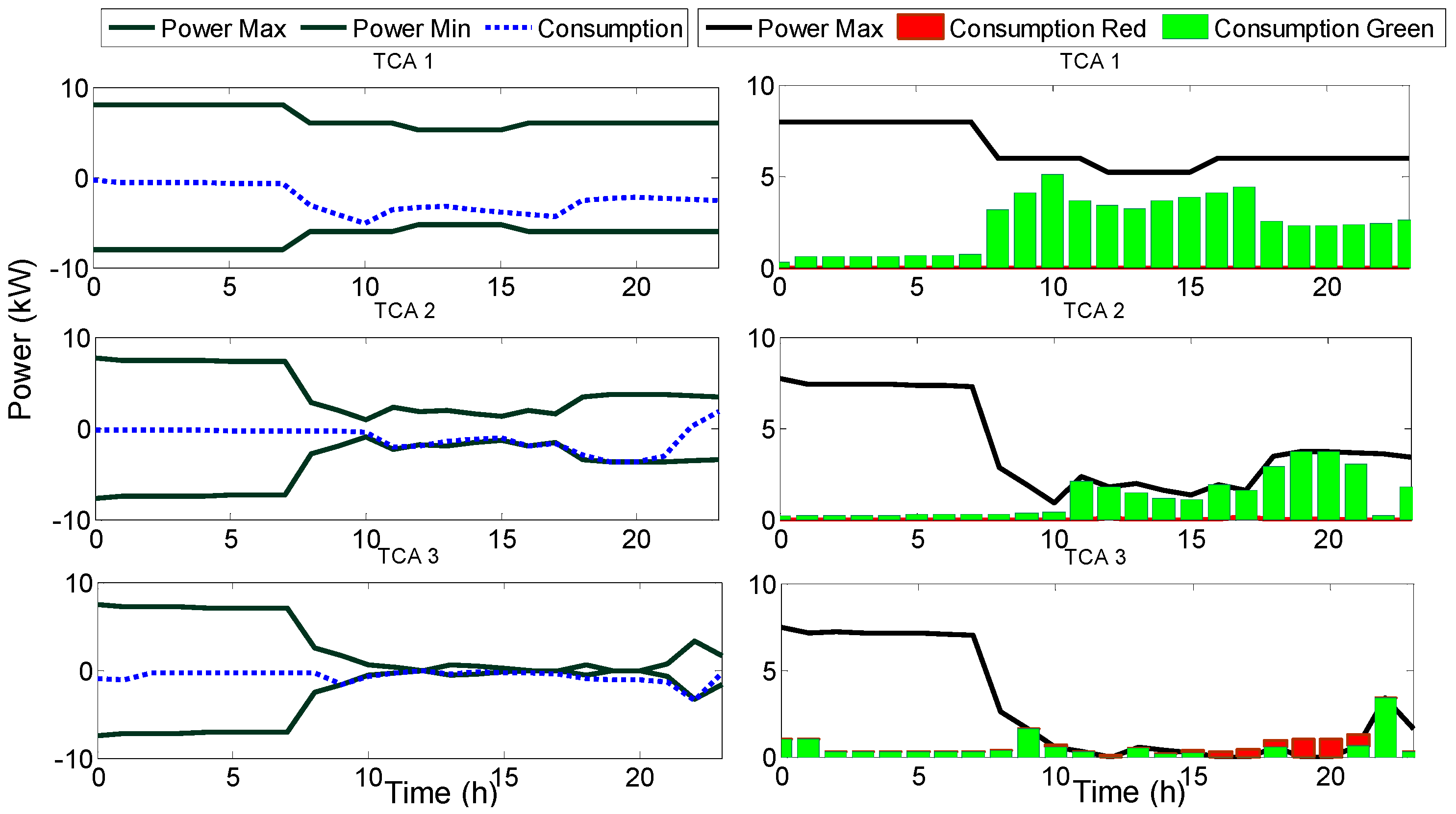
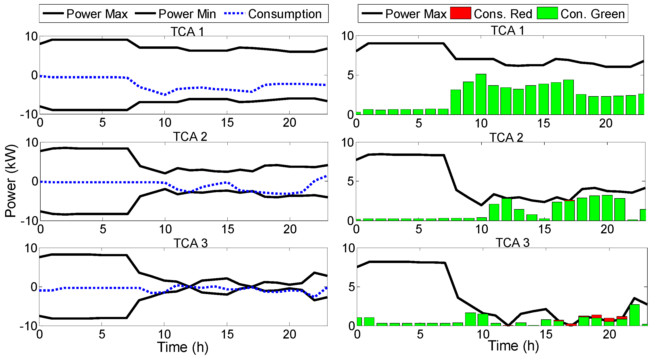
Despite the thermal disturbances presented in Figure 4b, it can be seen in Figure 5, that all of the indoor temperatures are predominantly inside their narrow bounds. This behavior is achieved as a result of the predictive knowledge of disturbance and by using space thermal storage. Thus, in the morning (for instance), the MPC precools the space’s temperature before the thermal load begins, namely until 08:00, 11:00, and 09:00 for TCA 1, TCA 2, and TCA 3, respectively. The precooling behavior also has the advantage of reducing the peak power consumption of the systems, as well as flattening the control profile. The same happens with the power consumption (Figure 6), which shows that the controllers only try to consume when the green resource is available; however, with TCA 3 being the last in the sequence, it merely receives the remaining resources, which, in several periods, does not oblige to the major consumption of the red resource. As mentioned, when the power consumption is negative, the space is cooled, and when it is positive, the space is heated. Consequently, in the left graphs of Figure 6, the green available resource for each TCA has a positive (power max) and negative (power min) boundary (${\underset{\_}{U}}_i=-{\overline{U}}_i$). In the right side of Figure 6, the consumption modulus is presented, and therefore, only the positive power boundary value is shown (power max). Also, the consumption value presented on the left side is described in terms of green and red. Note that, when the power constraint is not exceeded, only the clean resource is consumed, but when it is, the energy from the grid is used.

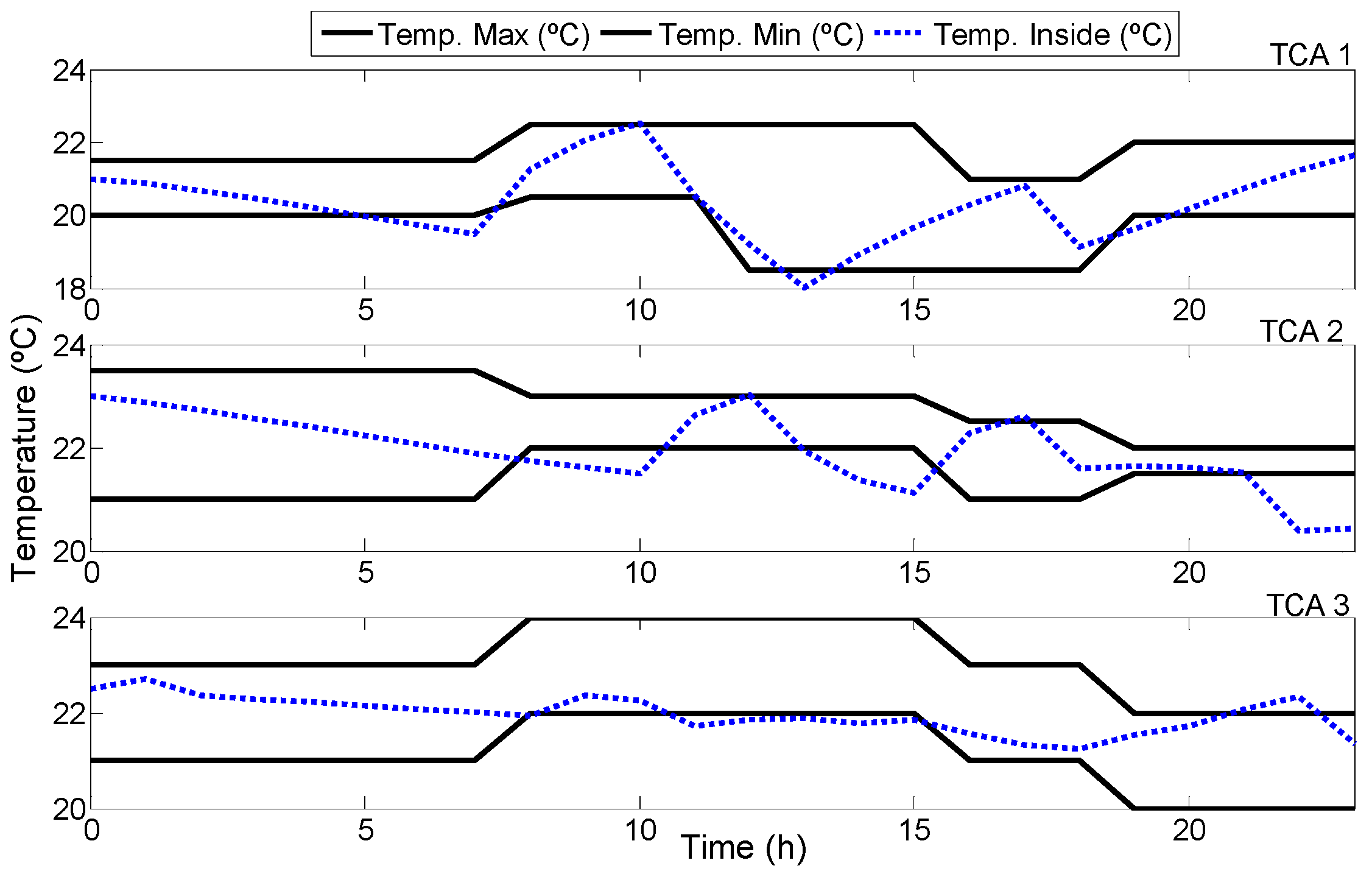
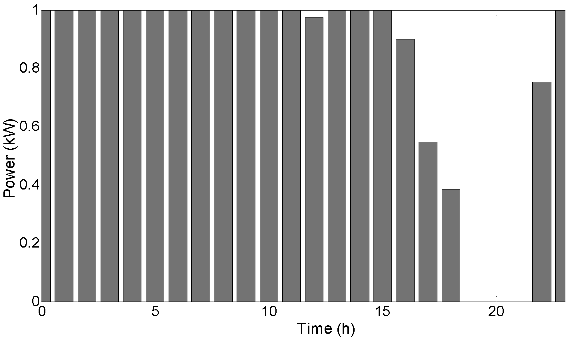
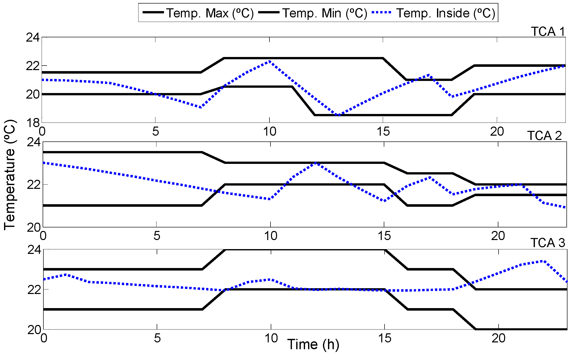
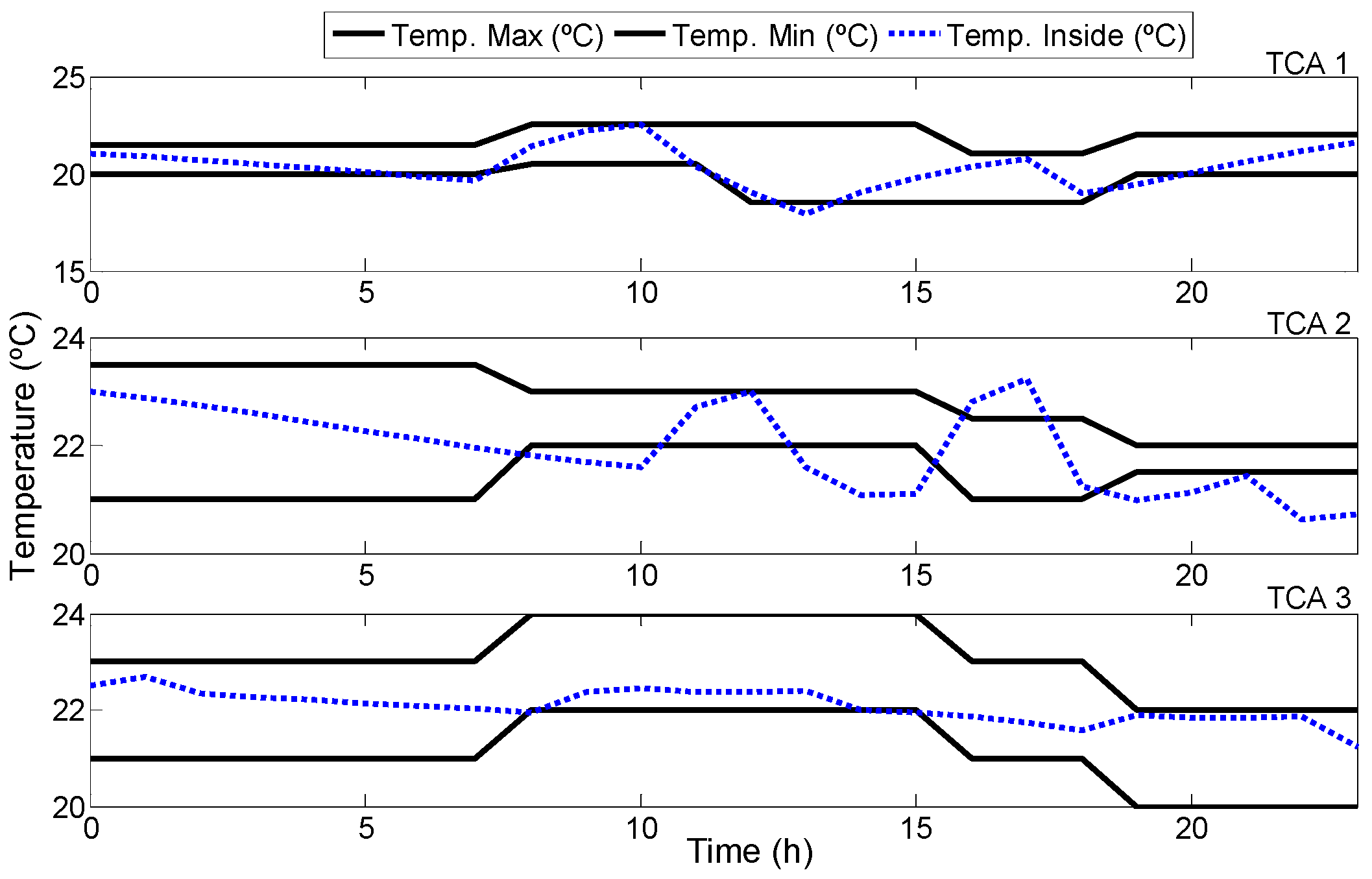
Scenario II is intended to show the benefit of having energy storage, with the only difference compared with Scenario I being the addition of a set of batteries with a 1.0 kWh of capacity. With this energy supplement provided by the batteries, compared with the previous scenario, the indoor temperature (Figure 8) had a minor deviation relative to the defined comfort gap.

Additionally, as expected, the power constraint of all of the agents was respected (Figure 9) except for in the interval between 17–21 h in TCA 3, where a small amount of the red resource was consumed.

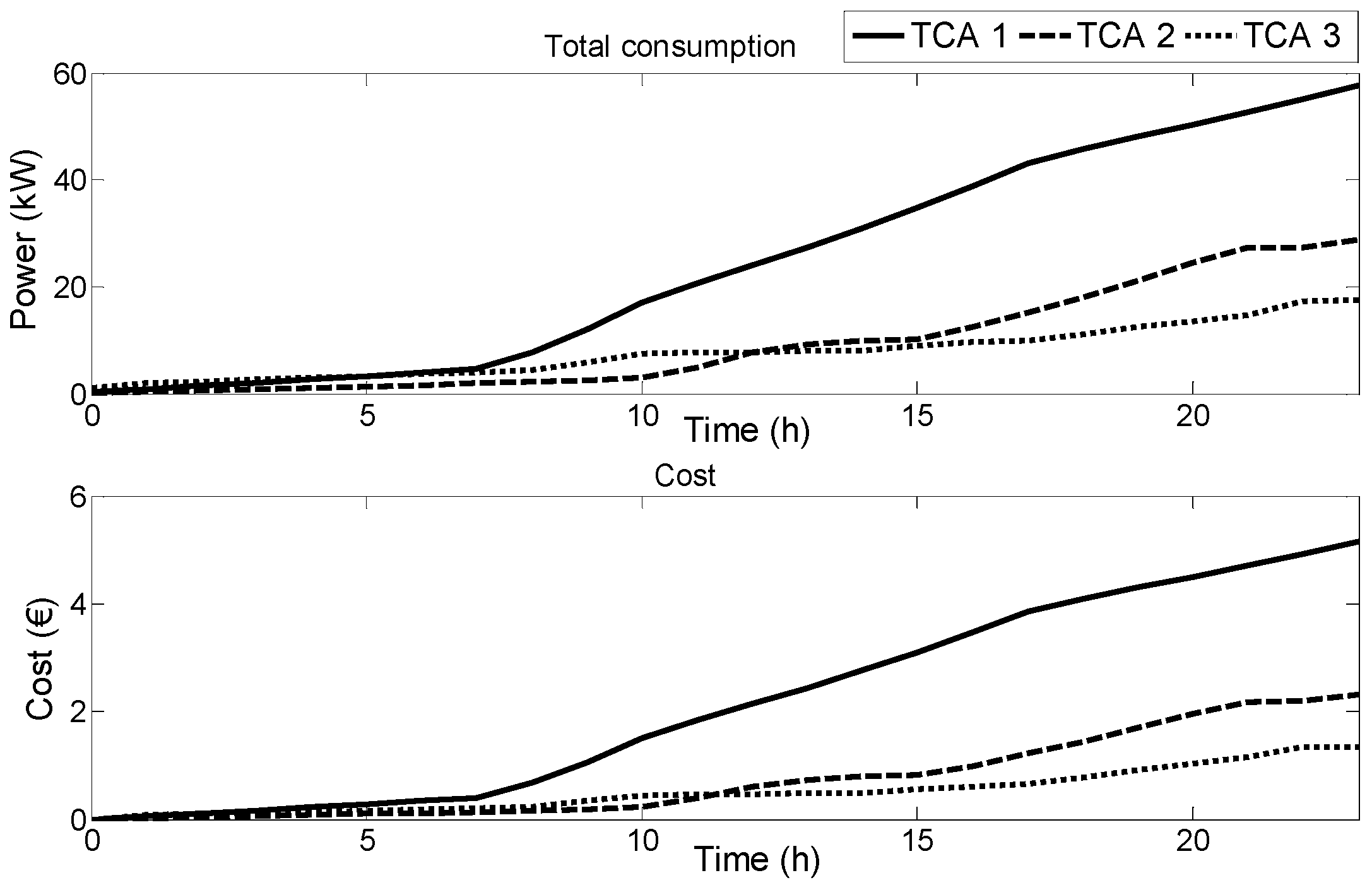
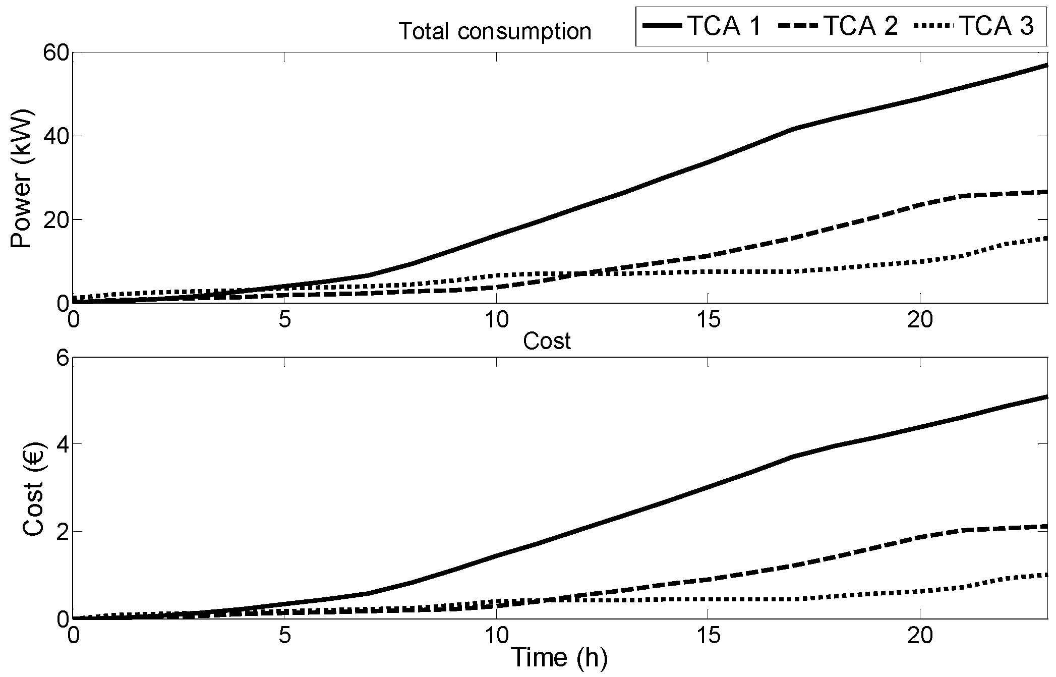
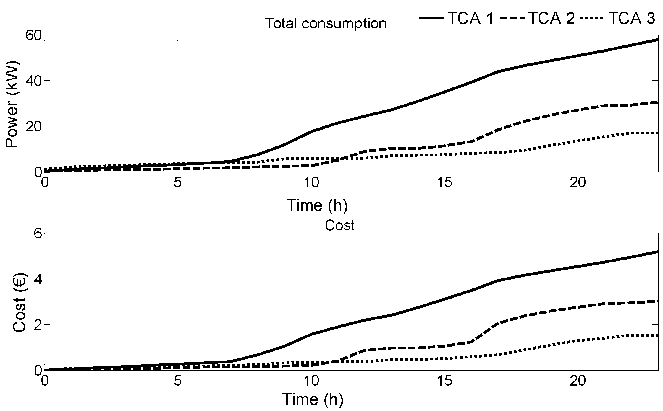
Compared with Figure 7, Figure 10 shows that consumption was reduced. The agent that most benefited from this modification was TCA 3, the energy surplus allowed for it to consume, almost exclusively, the green resource, bought at lower bid price, and thus, it presented the lowest cost. The batteries profile is presented in Figure 11.

In Scenario III, the penalty value of the parameters related to consumption were increased (

Table 3. Penalty values Scenario III.

Parameter	TCA 1	TCA 2	TCA 3
Comfort penalty—$\Xi$	50	50	50
Power penalty—ψ	100,000	100,000	30,000
Peak power penalty—$\varphi$	20	20	20
Consumption penalty—φ	10	10	10

).

Comfort is not relevant in this scenario (Figure 12), the agents are mostly concerned with reducing the consumption and complying with the power constraints. With this variation, the soft power constraint was transformed into a hard constraint, with the consumption profile continually maintained inside the bounds, meaning that no (or negligible) red resource was consumed (as shown in Figure 13). Therefore, compared with Scenario I, the consumption and energy costs, (Figure 14) were decreased in all of the agents. Because of its parameterization, TCA3 is obliged to consume only the available green resource, and for this reason, it showed a lower consumption and presented minor costs. Consequently, the TCA 3 indoor temperature was the one that was most penalized, presenting the highest deviation from the chosen temperature comfort gap.

The main focus of Scenario IV, for all of the TCAs, is the indoor temperature, as the comfort temperature range must be respected independently of the required energy consumption. Thus, the temperature penalty value was increased and the penalty value regarding consumption was decreased, as shown in

Table 4. Penalty values for Scenario IV.

Parameter	TCA 1	TCA 2	TCA 3
Comfort penalty—$\Xi$	50,000	50,000	50,000
Power penalty—ψ	1	1	3
Peak power penalty—$\varphi$	0.2	0.2	0.2
Consumption penalty—φ	0.1	0.1	0.1

.

As is seen in Figure 15, for all of the agents, the indoor temperature is mainly kept inside the temperature bounds, and consequently, the power constraints (Figure 16) are exceeded and the red resource consumption and cost has increased significantly (Figure 17).

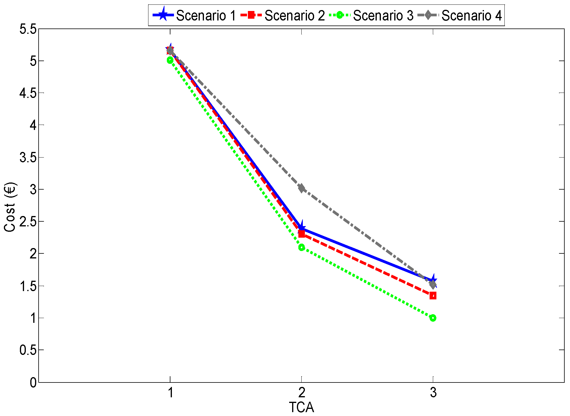
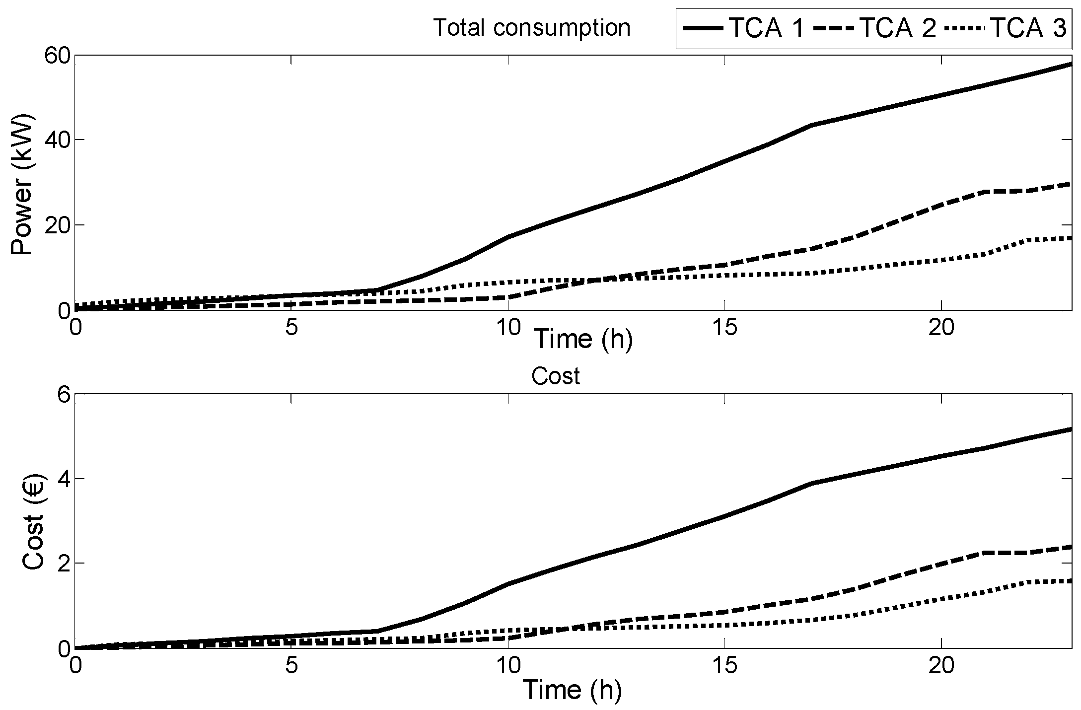
Distinct results were obtained in the proposed scenarios. Figure 18 summarizes the obtained costs for the 24 h simulation and ily heating/cooling total cost.

Table 5. Controller’s performance index.

Performance Index	TCA	Scenario I (Balanced Parameterization)	Scenario II (Balanced Parameterization with Batteries)	Scenario III (Less Consumption)	Scenario IV (More Comfort)
Comfort violation (Jε)	1	0.34	0.34	2.07	4.2 × 10−5
	2	2.07	1.28	2.81	3.9 × 10−4
	3	2.45	1.43	5.03	5.3 × 10−5
Power violation (Jγ)	1	4.7 × 10−7	4.5 × 10−7	9.7 × 10−9	2.3 × 10−3
	2	0.3	0.11	1.3 × 10−4	6.17
	3	4.29	1.75	0.01	3.71
Peak power consumption (JP)	1	0.26	0.33	0.56	0.23
	2	1.76	1.44	0.38	1.23
	3	0.06	0.27	0.025	0.05
Power consumption (Ju)	1	57.7	57.70	56.8	57.67
	2	29.66	28.81	26.48	30.35
	3	16.80	17.54	15.29	17.00

shows the controller’s performance index.

Comparing the economic differences between the scenarios, Scenario III was shown to be the most economical, with cost differences for TCA 1, TCA 2, and TCA 3 of less 2%, 13%, and 37%, respectively, when compared with Scenario I, and less 2%, 30%, and 35% when compared with Scenario IV, respectively. The parameters that penalized consumption were significantly increased, leading to a situation of less energy usage, and consequently, to a negligible power violation index, $J^{\gamma }$. However, this decreased consumption led to a higher indoor temperature deviation from the established boundaries, resulting in a comfort violation index, $J^{\epsilon }$, of 600%, 26%, and 52%, on the higher end compared with Scenario I for TCA 1, TCA 2, and TCA 3, respectively. On the other hand, Scenario IV was the most expensive. In this scenario, the penalty value in the temperature constraint was increased, showing that the consumers were only concerned about maintaining the temperature inside the boundaries. Thus, all of the required resources were consumed with respect to the temperature gap, leading to higher costs.

In several situations, comfort may be more relevant than cost, for example, in rooms with children, or in specific spaces in labs or hospitals that need to be accurately acclimatized. Nevertheless, even by prioritizing the indoor temperature, the minimization function (in due proportion, given by the penalty values) also minimizes the other terms. The parameterizations from the first and second scenarios were shown to be the most balanced, with a compromise between comfort and cost.

5. Conclusions

The developed scheme provides an integrated DSM solution for thermal comfort and energy efficiency, which optimally adjusts the demand to the supply and is based on distributed MPC techniques. The developed solution uses the thermal comfort area concept to define the agents that share information and that operate in a distributed environment. Each TCA solves its parameterized optimization problem with its own predictions, as well as with the information shared by its neighbors.

This was possible by using predictive control concepts and practices to develop the desired solution based on a distributed algorithm. The proposed solution contributes positively, with a methodology that allows for the design of new solutions that increase energy efficiency in the distribution networks, including the methods that involve demand-side management and prices.

The flexibility of the implemented scheme is shown compared with the different scenario results analysis. The system is able to obtain energy and cost savings (37%), and, as is also shown through the penalty index values, the user may restrict their consumption to the maximum that is available, or may choose to benefit from indoor comfort.

Taking advantage of the predictive knowledge of the disturbance and using the space thermal storage the controllers are able to precool the spaces, with the additional benefit of reduce the peak power consumption of the systems and smoother the control profiles.

The novel cost function optimization strategy is also suitable for application in scenarios where, simultaneously, the amount of energy is limited, and where comfort issues are also important and need to be taken into consideration.