Figure 1.
Maps showing bathymetry and coastlines for (a) the Orkney Islands, Scotland, and the location of the European Marine Energy Centre (EMEC) tidal energy test site (red rectangle). In (b), the region of the test site is expanded, and the deployment location of the TEC and multiple Diverging-beam Acoustic Doppler Profilers (D-ADP) deployments are identified as a yellow circle and further detailed in (c), where range rings (grey circles) commence at a radius of 40 m from TEC and increment every 10 m. (a) The Orkney Islands; (b) the EMEC tidal test site; (c) D-ADP deployments.
Figure 2.
The DeepGen-IV 1 MW tidal turbine being deployed from Hatston Quay, Kirkwall, Orkney. Sensor platforms Edinburgh Subsea Instrument Platform 1 (ESIP-1) and ESIP-2 visible on the turbine top of the main nacelle and the left rear on the thruster housing. Turbine hub-mounted Single-Beam (SB)-ADP position indicated (HUB), but not visible at this image angle.
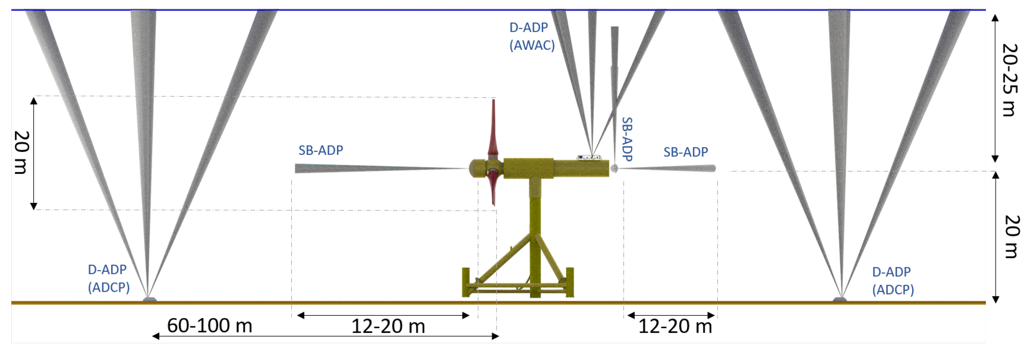
Figure 3.
Instrument layout on the DeepGen-IV tidal turbine. Acoustic beams are represented in grey.
Figure 3.
Instrument layout on the DeepGen-IV tidal turbine. Acoustic beams are represented in grey.
Figure 4.
Photograph of ESIP-1 showing: (1) the Converging Acoustic Doppler Profiler (C-ADP) system; (2,3) horizontally- and vertically-orientated SB-ADPs; (4) vertically-orientated D-ADP; (5) electronics’ subsea housing.
Figure 4.
Photograph of ESIP-1 showing: (1) the Converging Acoustic Doppler Profiler (C-ADP) system; (2,3) horizontally- and vertically-orientated SB-ADPs; (4) vertically-orientated D-ADP; (5) electronics’ subsea housing.
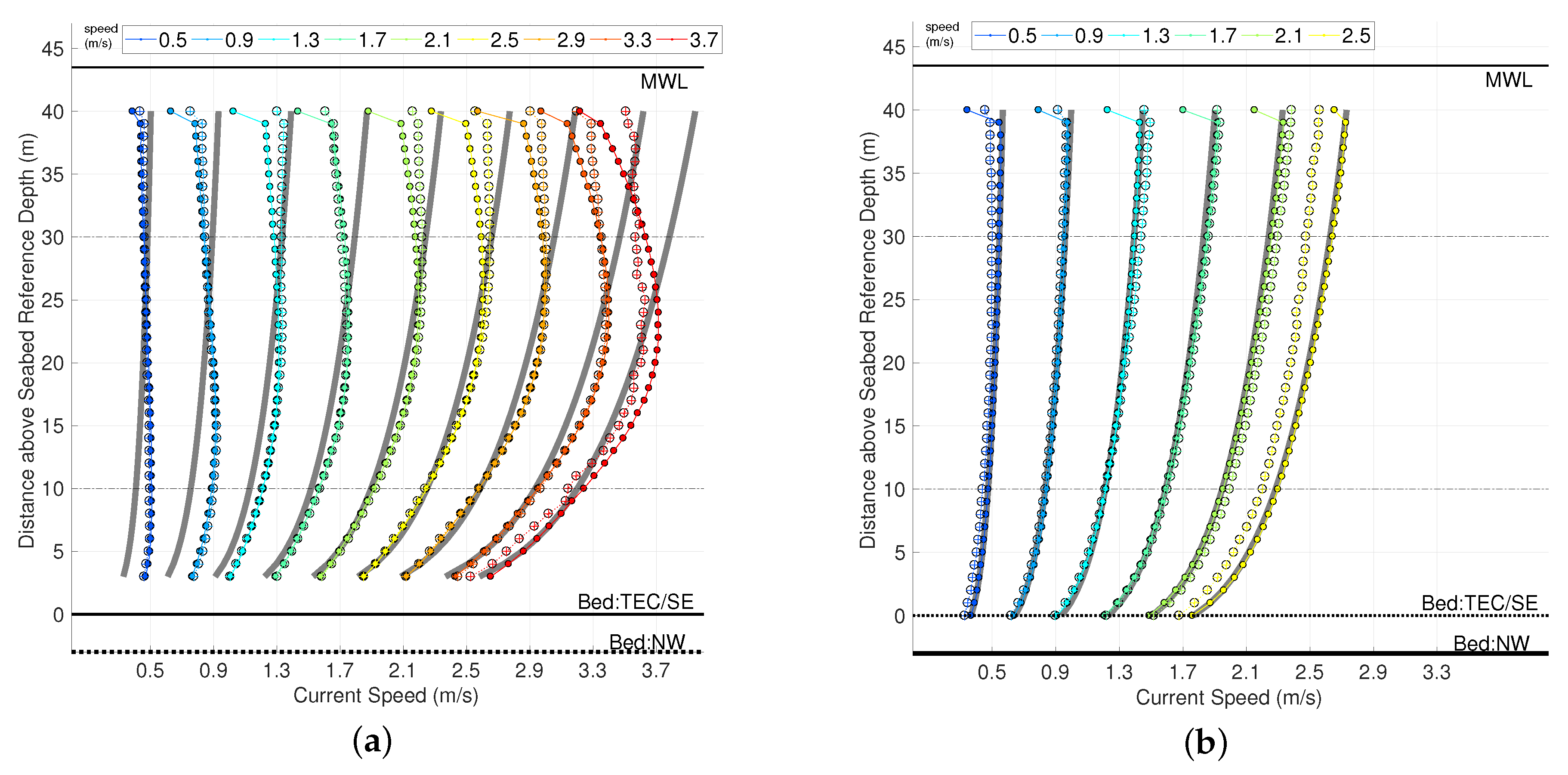
Figure 5.
Depth profiles of streamwise velocity for (a) ebb and (b) flood tide. Solid grey lines show power-law fit (). Small filled circles and large open circles with a centred cross show flows in the absence and presence of waves, respectively. Data is binned by speed as per the top horizontal legend. MWL shows mean water level. SE and NW indicate depths at southeast and northwest positions. (a) Ebb tide streamwise velocity depth profiles. (b) Flood tide streamwise velocity depth profiles.
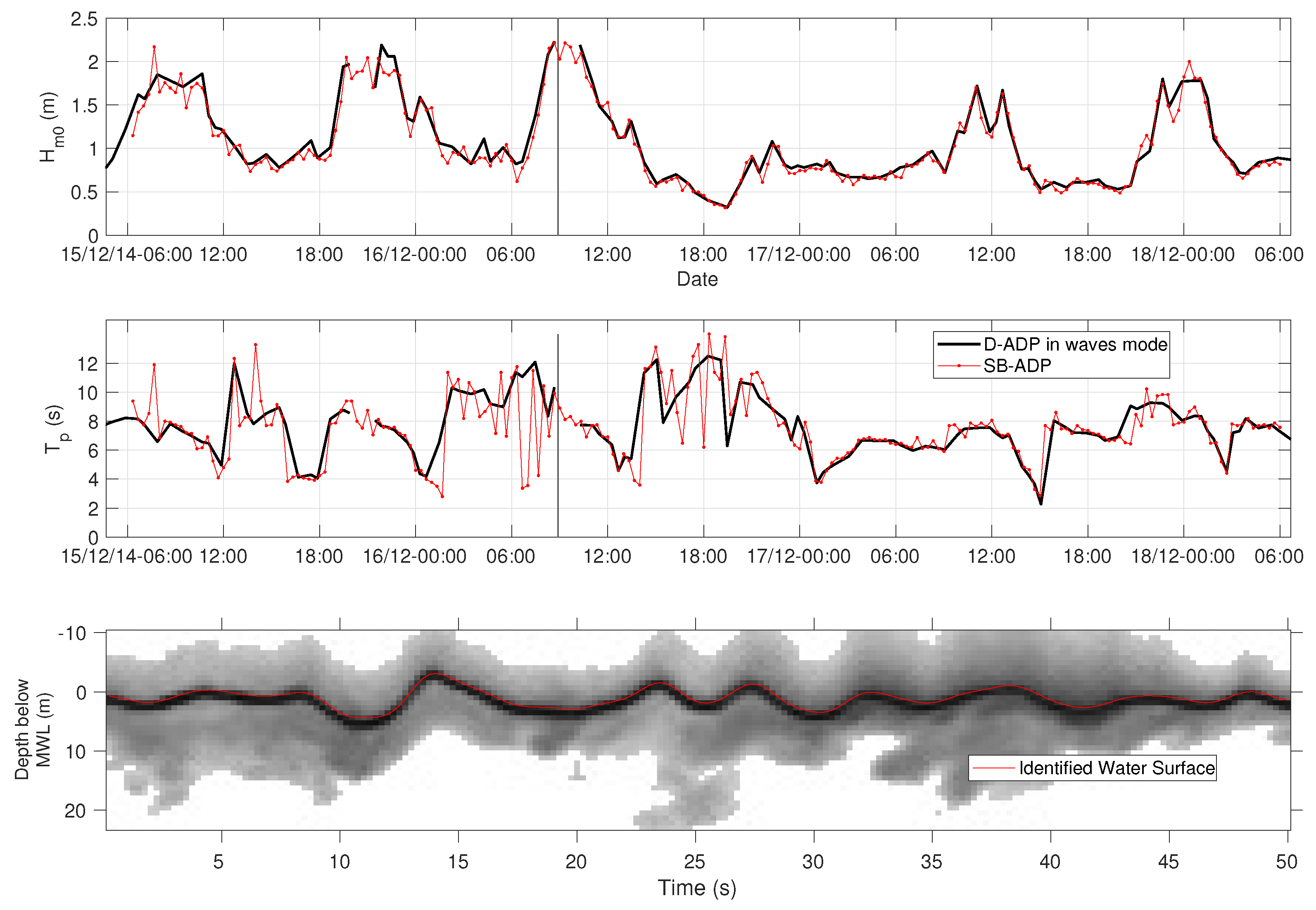
Figure 6.
Time series (15–18 December 2014) of significant wave height, (top), and peak period, (middle), as measured above the TEC by (black line) the benchmark instrument, the AWAC D-ADP operating in “waves mode” and (red line) a vertically-orientated SB-ADP. The vertical grey line shows the starting time of an example surface tracking analysis (bottom) showing the background amplitude return signal from the SB-ADP and the corresponding detected surface (red line).
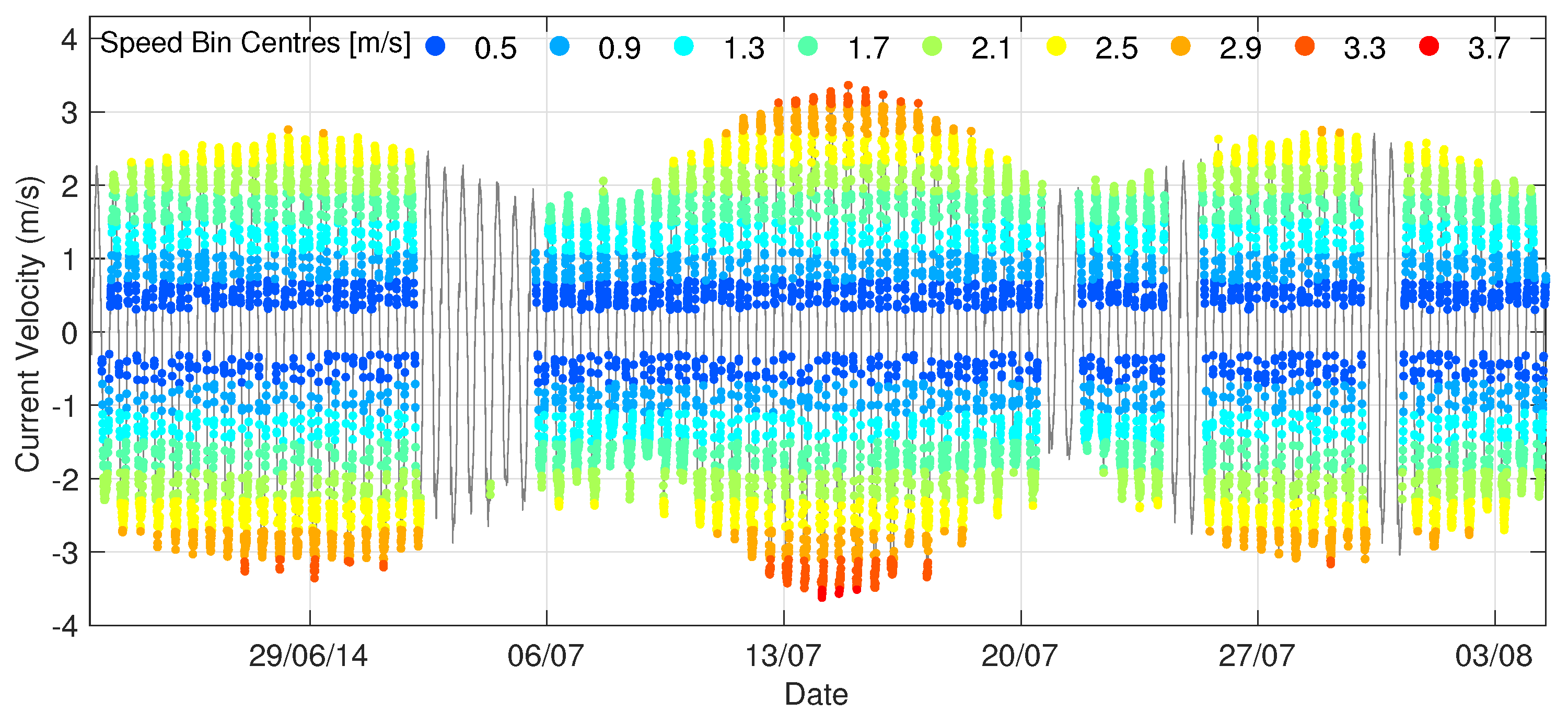
Figure 7.
Time series of velocity data (June–July 2014) acquired by an upstream D-ADP. Filtered data are shown segregated by speed bin-centres (graduated colours). The grey line shows all acquired data: gaps represent excluded data where significant wave height, , exceeds the 0.8-m threshold.
Figure 7.
Time series of velocity data (June–July 2014) acquired by an upstream D-ADP. Filtered data are shown segregated by speed bin-centres (graduated colours). The grey line shows all acquired data: gaps represent excluded data where significant wave height, , exceeds the 0.8-m threshold.
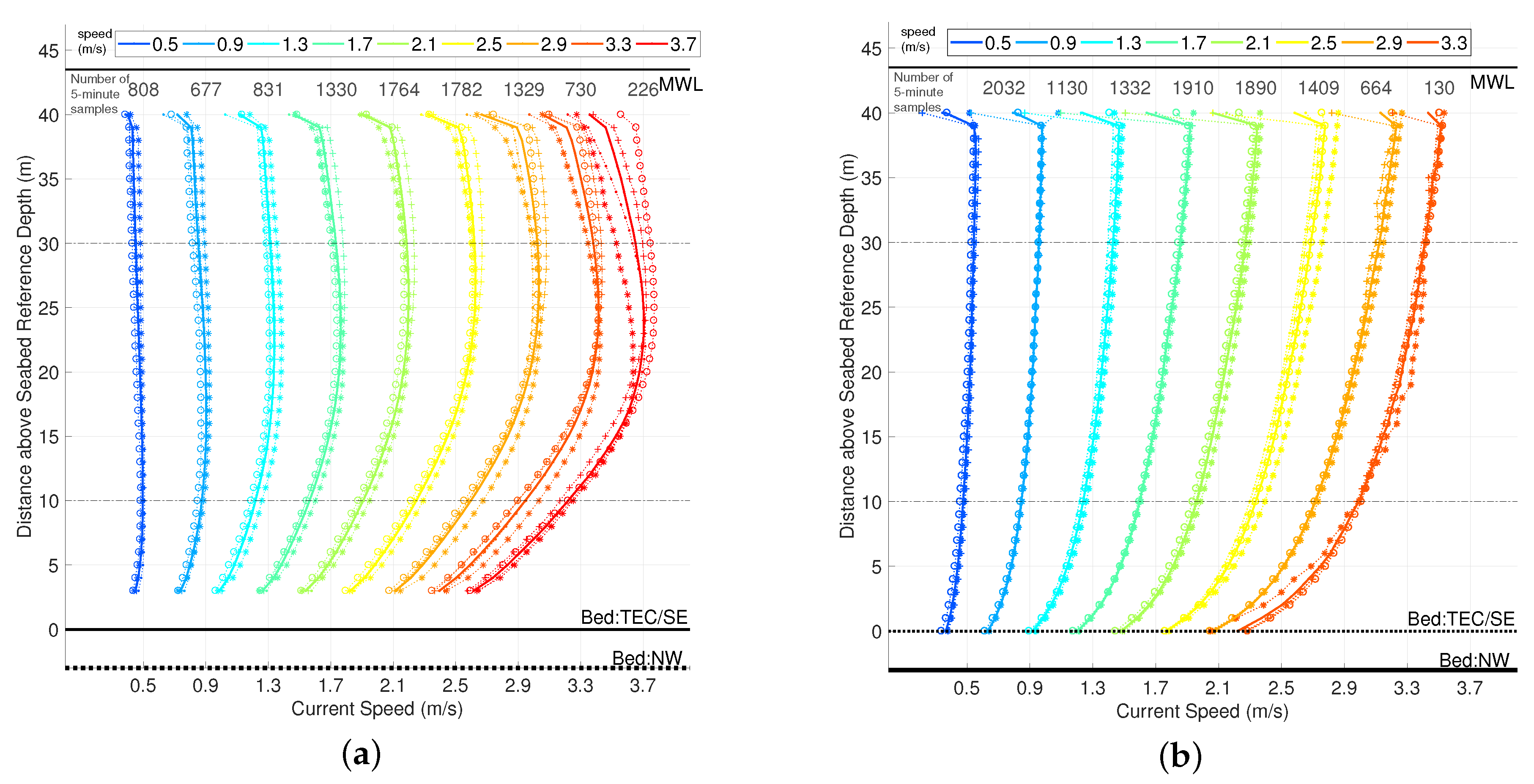
Figure 8.
Depth profiles of streamwise velocity for (a) ebb tide and (b) flood tide. Measurements from individual deployments are shown with distinct markers. Solid lines without markers present the average flow speed across instruments for a given speed bin. (a) Ebb tide streamwise velocity depth profiles. (b) Flood tide streamwise velocity depth profiles.
Figure 9.
Depth profiles of streamwise velocity for (a) ebb tide and (b) flood tide. Measurements are averages across all available instruments. Upwards-pointed chevrons show depth profiles corresponding to periods of positive flow acceleration; downwards-pointed chevrons show depth profiles corresponding to periods of negative flow acceleration. (a) Aggregate ebb tide velocity depth profiles with additional acceleration binning. (b) Aggregate flood tide velocity depth profiles with additional acceleration binning.
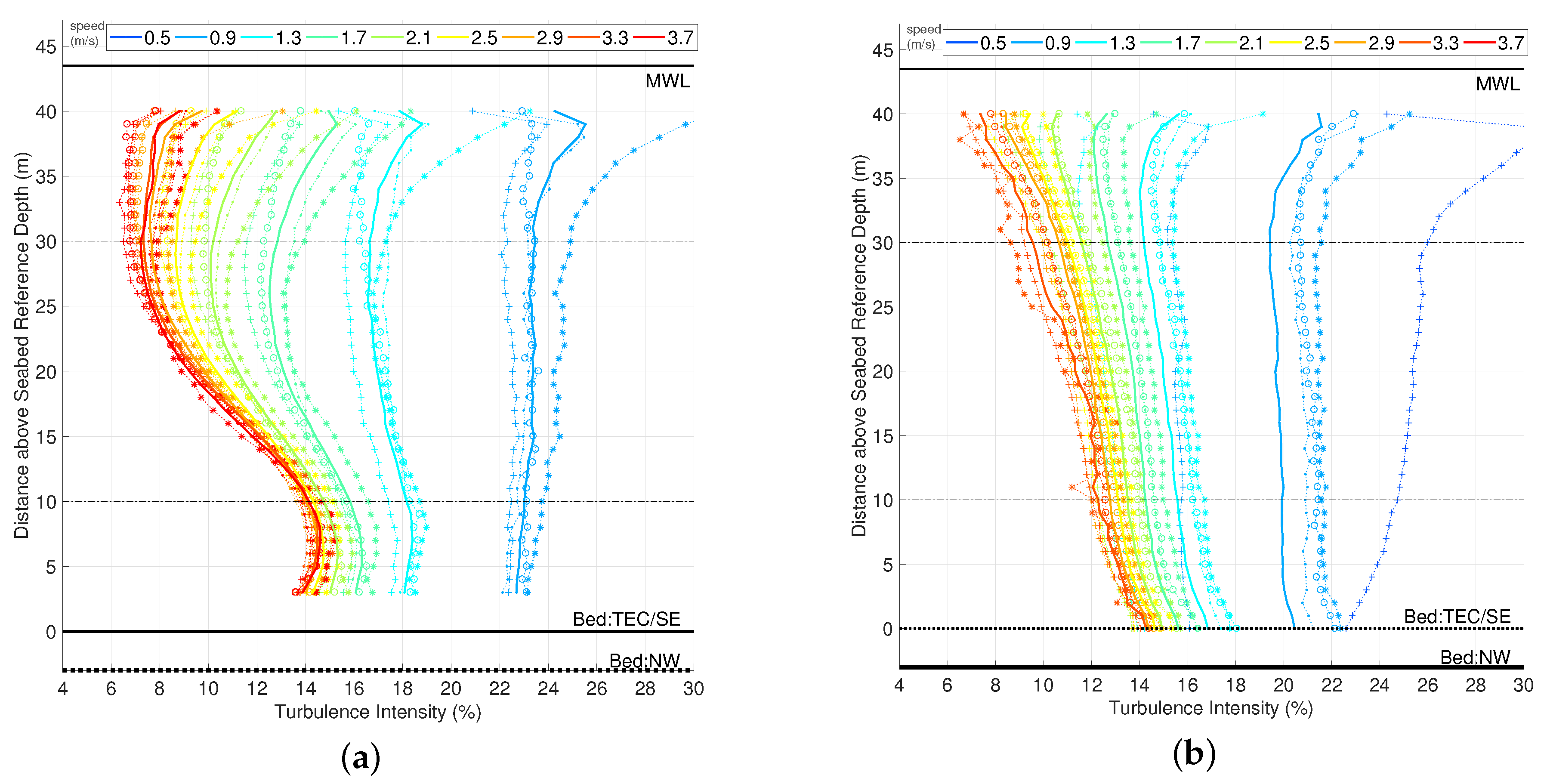
Figure 10.
Depth profiles of turbulence intensity for (a) ebb tide and (b) flood tide. Values, averaged over five minutes and binned by speed, from individual sensor deployments are shown with distinct markers: open circles, stars, pluses and small closed circles. Solid lines without markers present the average TI across these separate deployments for a given speed bin (shown in the top horizontal legend). (a) Ebb tide TI depth profiles. (b) Flood tide TI depth profiles.
Figure 11.
Aggregate (averaged over four instrument deployments per tide) depth profiles of TI for (a) ebb and (b) flood tides with noise correction implemented. Profiles featuring noise correction are marked by filled circles: uncorrected raw profiles are shown as crosses. (a) Aggregate ebb tide TI depth profiles. (b) Aggregate flood tide TI depth profiles.
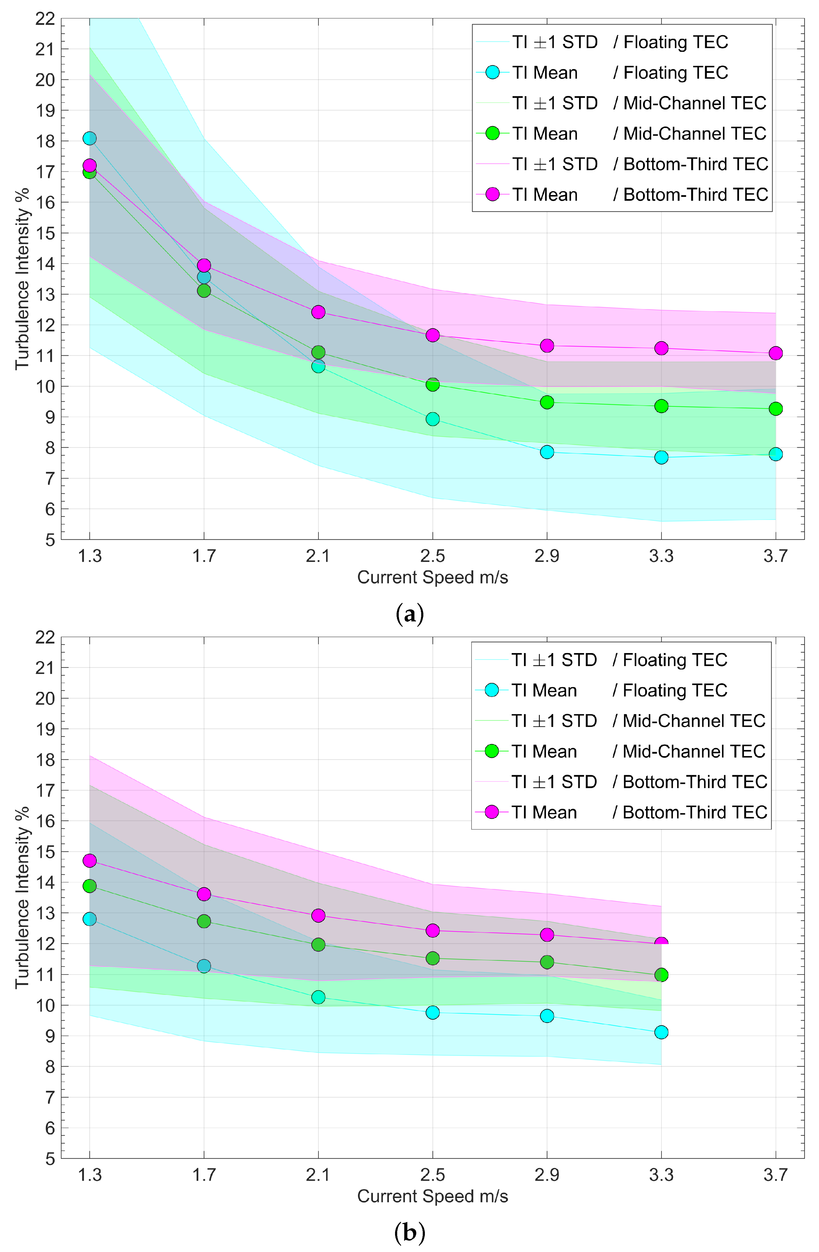
Figure 12.
Spatially-averaged TI against current speed for (
a) ebb and (
b) flood tides and corresponding levels of variation (shown as ± one standard deviation (STD)) across the specific vertically-sampled region for the three TEC installation types described in
Table 3. (
a) Ebb tide TI variation with speed. (
b) Flood tide TI variation with speed.
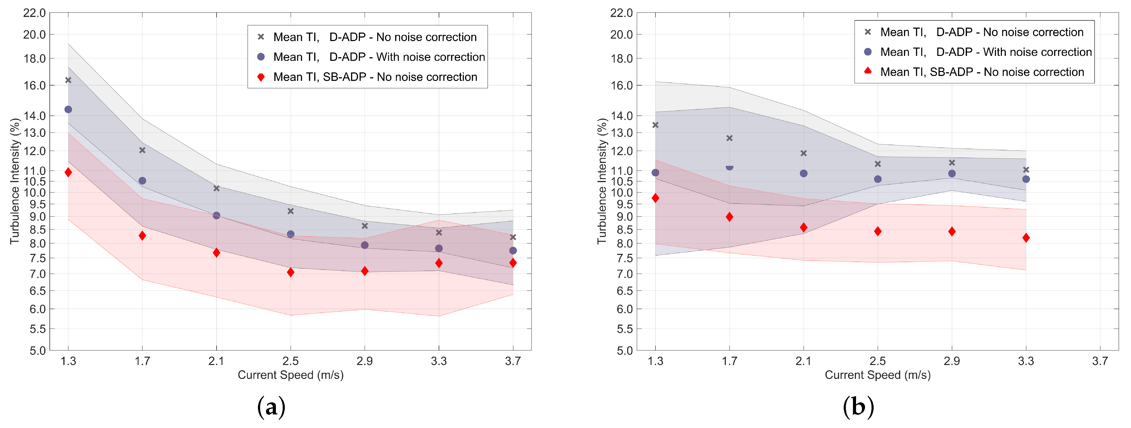
Figure 13.
Turbulence intensity against current speed for (a) ebb and (b) flood tides. Filled circles show mean values of TI per velocity bin derived from noise-corrected D-ADP data. Crosses show equivalent uncorrected values. Mean values of TI measured at hub-height via SB-ADP are marked with red diamonds. Shaded areas, matching mean-marker colours, represent plus and minus one standard deviation from these means. (a) Ebb Tide TI via D-ADP and SB-ADP. (b) Flood Tide TI via D-ADP and SB-ADP.
Table 1.
Turbine-proximal deployments of D-ADPs showing unique campaign ID, date deployed and duration of deployment. Locations are shown in
Figure 1c. Due to a memory card error, no data were retrieved from the Deployment (Dep) 4 “NW”.
Table 1.
Turbine-proximal deployments of D-ADPs showing unique campaign ID, date deployed and duration of deployment. Locations are shown in
Figure 1c. Due to a memory card error, no data were retrieved from the Deployment (Dep) 4 “NW”.
| ID | D-ADP Name | Date Deployed | Duration Days | ID | D-ADP Name | Date Deployed | Duration Days |
|---|
| 0 | 01_NW_Dep0 | 2013-02-21 | 24 | 4 | 02_NW_Dep4 | 2014-04-09 | 0 |
| 1 | 01_NW_Dep1 | 2013-06-05 | 42 | 4 | 02_SE_Dep4 | 2014-04-09 | 58 |
| 1 | 02_SE_Dep1 | 2013-06-05 | 42 | 5a | 03_SE_Dep1 | 2014-06-20 | 46 |
| 2 | 01_NW_Dep2 | 2013-07-18 | 15 | 5a | 01_NW_Dep5 | 2014-06-22 | 41 |
| 2 | 02_SE_Dep2 | 2013-07-18 | 15 | 5b | 02_NW_Dep5 | 2014-07-07 | 40 |
| 3 | 01_NW_Dep3 | 2013-10-15 | 42 | 6a | TD7_01_Dep1 | 2014-09-17 | 85 |
| 3 | 02_SE_Dep3 | 2013-10-15 | 40 | 6b | TD7_02_Dep1 | 2014-09-17 | 71 |
Table 2.
Acoustic instrument summary specification.
Table 2.
Acoustic instrument summary specification.
| Instrument Name (Manufacturer) | Acoustic Frequency (kHz) | Type | Sample Rate (Hz) | Quantity | Location |
|---|
| ADCP (RDI) | 600 | D-ADP | 0.5–2 | 2 | Seabed near-TEC |
| AWAC (Nortek) | 1000 | D-ADP | 1 | 1 | Turbine ESIP-1 |
| AD2CP (Nortek) | 1000 | SB-ADP | 1–4 | 16 | Turbine ESIP-1&2 |
| Continental (Nortek) | 192 | SB-ADP | 1 | 1 | Turbine ESIP-2 |
| AD2CP (Nortek) | 1000 | SB-ADP | 1–4 | 1 | Turbine Hub Centreline |
Table 3.
Spatial averaging regions in the vertical direction for three TEC installation types and a narrow mid-depth sampling regime. Distances are relative to the seabed.
Table 3.
Spatial averaging regions in the vertical direction for three TEC installation types and a narrow mid-depth sampling regime. Distances are relative to the seabed.
| Turbine Installation Type | Range from Seabed (m) | Rotor Diameter (m) |
|---|
| TEC Floating | 20–38 | 18 |
| TEC Mid-Depth | 10–30 | 20 |
| TEC Deep (Bottom Third) | 9–21 | 12 |
| Channel Mid-Depth | 19–21 | N/A |
Table 4.
Correction factors reported as the standard deviation in cm/s due to sensor noise for turbine-mounted SB-ADP and seabed-mounted D-ADP data in the absence of waves.
Table 4.
Correction factors reported as the standard deviation in cm/s due to sensor noise for turbine-mounted SB-ADP and seabed-mounted D-ADP data in the absence of waves.
| Sensor | Direction | Flood (cm/s) | Ebb (cm/s) |
|---|
| SB-ADP | U | 6.2 | 6.2 |
| D-ADP | U | 10.1 | 10.3 |
Table 5.
Streamwise Turbulence Intensity (TI) values with and without data exclusion based on contemporaneous wave measurement for a single summer D-ADP deployment. TI is a relative percentage difference.
Table 5.
Streamwise Turbulence Intensity (TI) values with and without data exclusion based on contemporaneous wave measurement for a single summer D-ADP deployment. TI is a relative percentage difference.
| | Ebb Tide | Flood Tide |
|---|
| | | All Data | TI | | All Data | TI |
|---|
| Floating TEC | 8.4 | 9.2 | 9.0 | 9.7 | 9.8 | 1.2 |
| Mid-Depth | 9.4 | 9.6 | 2.5 | 11.4 | 11.4 | 0.3 |
Table 6.
TI with and without noise correction for differing TEC deployment depths. Std is the standard deviation derived spatially across the vertical range.
Table 6.
TI with and without noise correction for differing TEC deployment depths. Std is the standard deviation derived spatially across the vertical range.
| Turbine Installation Type | Noise Correction | TI (%) at Three Flow Speed Ranges (m/s) |
|---|
| 0.3 < U < 3.9 | 1.1 < U < 3.9 | 1.9 < U < 3.9 |
|---|
| Mean Std | Mean Std | Mean Std |
|---|
| D-ADP ebb tide | | | | | | | |
| Floating | No | 14.4 | 11.3 | 10.7 | 5.4 | 9.1 | 4.0 |
| Floating | Yes | 12.8 | 10.1 | 9.4 | 5.3 | 8.1 | 4.1 |
| Mid-Depth | No | 14.7 | 9.4 | 11.3 | 2.9 | 10.1 | 1.5 |
| Mid-Depth | Yes | 12.9 | 7.7 | 10.3 | 2.7 | 9.3 | 1.5 |
| Deep (Bottom Third) | No | 15.6 | 8.3 | 12.7 | 2.3 | 11.7 | 1.3 |
| Deep (Bottom Third) | Yes | 13.9 | 6.5 | 11.7 | 2.1 | 11.0 | 1.3 |
| Channel Mid-Depth | No | 13.7 | 9.8 | 10.3 | 3.2 | 9.0 | 1.5 |
| Channel Mid-Depth | Yes | 12.0 | 8.2 | 9.2 | 3.0 | 8.1 | 1.6 |
| D-ADP flood tide | | | | | | | |
| Floating | No | 15.4 | 9.4 | 10.8 | 2.1 | 10.0 | 1.3 |
| Floating | Yes | 12.5 | 7.8 | 9.5 | 2.2 | 9.1 | 1.4 |
| Mid-Depth | No | 16.7 | 9.0 | 12.4 | 2.1 | 11.7 | 1.3 |
| Mid-Depth | Yes | 13.7 | 7.2 | 11.1 | 2.2 | 10.9 | 1.4 |
| Deep (Bottom Third) | No | 17.5 | 9.1 | 13.3 | 2.2 | 12.6 | 1.5 |
| Deep (Bottom Third) | Yes | 14.5 | 7.3 | 12.0 | 2.3 | 11.8 | 1.6 |
| Channel Mid-Depth | No | 16.4 | 9.0 | 12.2 | 2.8 | 11.5 | 1.8 |
| Channel Mid-Depth | Yes | 13.5 | 7.4 | 11.0 | 2.9 | 10.7 | 1.9 |
| SB-ADP ebb tide | | | | | | | |
| Channel Mid-Depth | No | 10.8 | 6.1 | 7.9 | 1.9 | 7.3 | 1.3 |
| SB-ADP flood tide | | | | | | | |
| Channel Mid-Depth | No | 11.9 | 6.3 | 8.8 | 1.4 | 8.5 | 1.1 |

 ,
, 


