Article

Cyclic Experimental Studies on Damage Evolution Behaviors of Shale Dependent on Structural Orientations and Confining Pressures

1
Key Laboratory of Shale Gas and Geoengineering, Institute of Geology and Geophysics, Chinese Academy of Sciences, Beijing 100029, China
2
Institutions of Earth Science, Chinese Academy of Sciences, Beijing 100029, China
3
College of Earth Sciences, University of Chinese Academy of Sciences, Beijing 100049, China
*
Author to whom correspondence should be addressed.
Energies 2018, 11(1), 160; https://doi.org/10.3390/en11010160
Submission received: 24 November 2017 / Revised: 29 December 2017 / Accepted: 3 January 2018 / Published: 9 January 2018
(This article belongs to the Section L: Energy Sources)

Abstract

:
Damage process of shale is of great importance when considering the wellbore stability and reservoir stimulation during the work of shale gas recovery. As shale has typical transversely isotropic structures and may be under different stress states in the reservoir, the damage process should be studied while considering both loading directions and confining pressures. A series of cyclic uniaxial and tri-axial compressive tests have been carried out on the shale samples with different oriented weak planes and confining pressures. The dissipated strain energy and its ratio to the releasable elastic strain energy have been studied comparing with the fracturing patterns of the samples. Based on the strain energy dissipation, damage variable is defined and the damage evolution equation is built to describe the damage process of shale samples dependent on loading directions and confining pressures. The damage equation shows that the damage of the shale samples increases as a power function of the axial stress. Under higher confining pressures, the damage is limited in the early loading stage, while it increases significantly with the formation of macro shear fractures when the peak strength is approaching. The change of increasing rate is weak for the shale samples (β = 60°) as the main failure pattern is slip along the weak planes. This study is helpful for understanding the damage process and failure of wellbore, as well as the stimulation effect of the shale gas reservoir.

1. Introduction

Wellbore stability and reservoir stimulation are both of great paramount during the process the shale gas recovery [1,2]. Damage behaviors of shale are very important to understand the failure and deformation of the wellbore, as well as the fracturing propagation, permeability change in the shale reservoirs [3,4,5]. There have been many theoretical studies on the rock with structural planes, including the strength criterion [6,7,8,9,10], and constitutive relationships [4,11,12]. However, the strength criterion cannot consider the damage process of the rock, and the constitutive relationships are always built based on some assumptions and they need the examination by the experimental results. Consequently, the experimental studies on the damage process of the shale are very important.
Damage characteristics of rock have been widely researched based on many different methods. With the development of experimental techniques, Acoustic emission, wave velocity, CT scanning, electric and magnetic methods, etc. have been used to describe the damage process of the rock specimens under different loading or unloading conditions [13,14,15,16,17]. Different parameters, like the Young’s modulus, accumulated plastic strain, dissipated strain energy, AE hits, CT number, wave velocity, etc. have been used to define the damage variable [13,14,15,16,18,19,20,21,22,23,24]. With the suitable damage variable, different kinds of damage evolution equations have been built, and some constitutive equations have also been developed [18].
However, these studies mainly focus on the rock specimens with almost isotropic structures. It is still not clear about the damage process of shale with different oriented weak planes. What is more, when considering the depth of the reservoir, the different in situ stresses owing to the geological tectonics, and the distance from the wellbore drilling, the shale may be under different stress states [25]. For example, Barnett shale reservoir of the Fort Worth Basin, Texas has the depth of generally 6500–8500 ft (1981–2591 m) [26], and Haynesville shale reservoir in Northeast Texas and Northwest Louisiana has the depth ranging from 10,000 to 14,000 ft (3048–4267 m) [27]. Consequently, the structural orientation and confining pressures should both be considered to study the damage process of the shale.
In the recent decades, energy analysis has been more and more applied in studying the failure and deformation behaviors of rock [21,22,23,24,28,29,30,31,32]. The previous studies based on theoretical analyses and experiments have shown that the evolution of energy plays an important role in the deformation and failure process of different types of rock [21,23]. Especially, it is found that the dissipation of energy associates with the formation of new fracturing surfaces, and the transferring of the stored strain energy may cause the strength weakness of the materials [33]. It is also shown that energy analysis is a relatively simple method to study the damage process of rock with clear and reasonable physical meanings [23]. The cyclic loading and unloading experiments are usually used for analyzing the energy evolution and damage process [18,23,28]. This type of test have very limited numbers cycles with very low frequency when compared with the fatigue test, and the damage induced by the cycles can be ignored.
Here, in this study, the cyclic loading and unloading experiments under different confining pressures were carried out on the shale samples with different oriented weak planes (Section 2); the energy characteristics were studied (Section 3). Based on the energy dissipation, damage variable was defined and the damage evolution behaviors were described (Section 4). This study considers both the structural direction and confining pressures, and the obtained damage behaviors should be useful for understanding the wellbore stability and the reservoir stimulation in the shale gas recovery.

2. Samples, Experimental Setup and Method
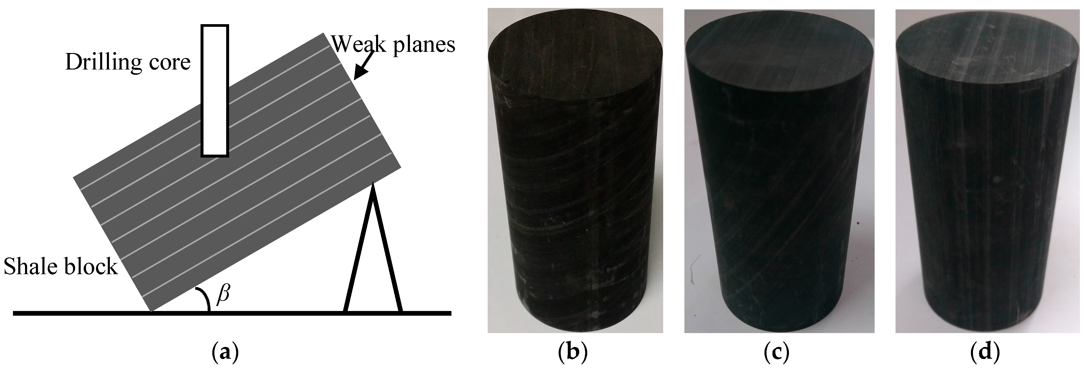
2.1. Samples

The shale specimens were grabbed from an outcrop of Longmaxi formation from Chongqing, China. The intact samples are generally black in color with natural parallel weak planes. Figure 1a presents the coring method at different directions relative to the weak planes. The cylindrical shale samples were prepared with the size of 50 mm in diameter and 100 mm in height, as well as various inclination angles of β = 30°, 60°, 90°, i.e., the acute angle between the weak planes and the end of the specimens (the direction of σ3 in triaxial compression tests) (Figure 1b–d). It should be noted that β = 0° is also an important case for studying. However, as this type of shale is very easy to disintegrate during the drilling and cutting with water, very limited numbers of samples can be prepared successfully. After an extensive review on the previous studies [4,8,34,35,36,37,38,39], we found that the fracturing patterns are quite similar (fracturing crossing the weak planes) for many types of shale samples with β = 0° and 30°, because the slip along the weak planes is not easy to occur, and the failure is always dominated by the strength of the rock material for the samples with such low inclination angles. Consequently, based on the limited numbers of shale samples, the inclination angles of β = 30°, 60°, 90° can be considered as three typical cases for studying the damage behaviors of shale with weak planes. More detailed analyses on the shale samples with more inclination angles will be conducted in the future studies.
The bulk density and P-wave velocity of each of the samples are presented in Table 1. Bulk density ρ is calculated with the samples dried in the air in room temperature for seven days as ρ = m/(πr2H) (m, r, and H are the mass, radius, and height of the cylindrical samples, respectively). P-wave velocities of the samples were measured with NM-3C ultrasonic wave monitoring system (Figure 2a) in Key Laboratory of Shale Gas and Geoengineering, Chinese Academy of Sciences, Beijing. A pair of transducers (Figure 2b) is attached to the two ends of each sample for transmitting and receiving P-wave signals. The P-wave velocity Vp can be calculated as Vp = H/t (H is the height of each sample and t is the transmission time of the wave). The P-wave velocities of the samples are plotted in Figure 2c and the anisotropic characteristics can be observed.

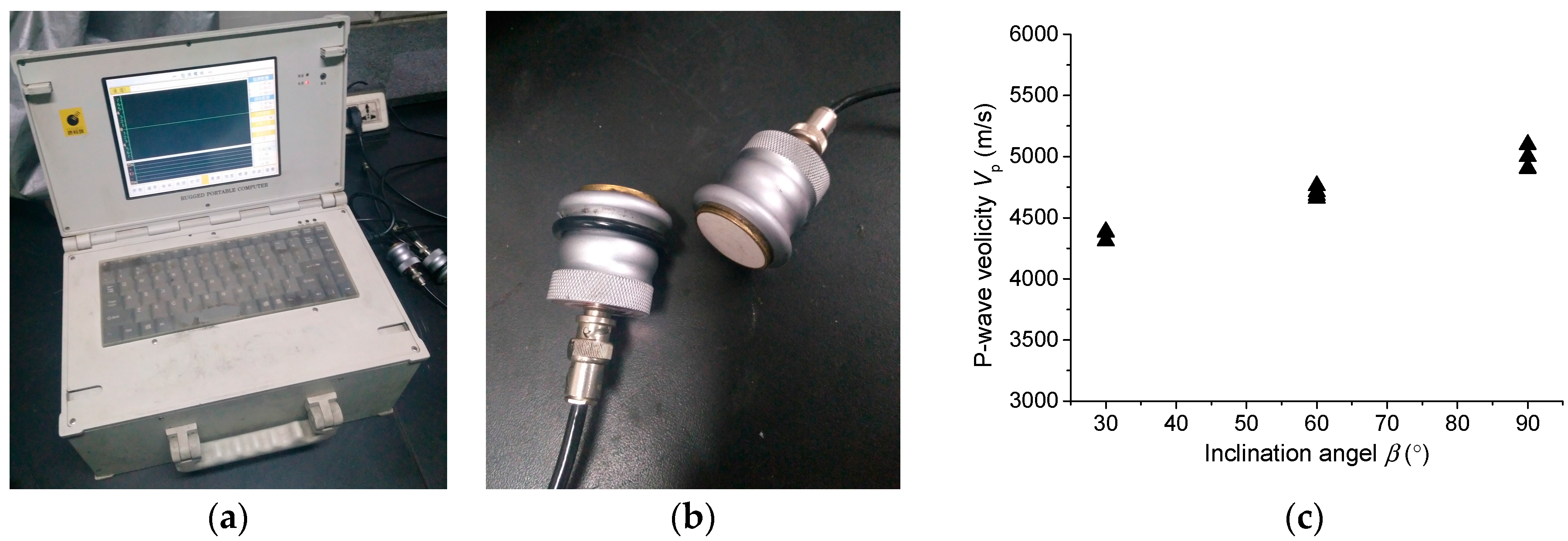
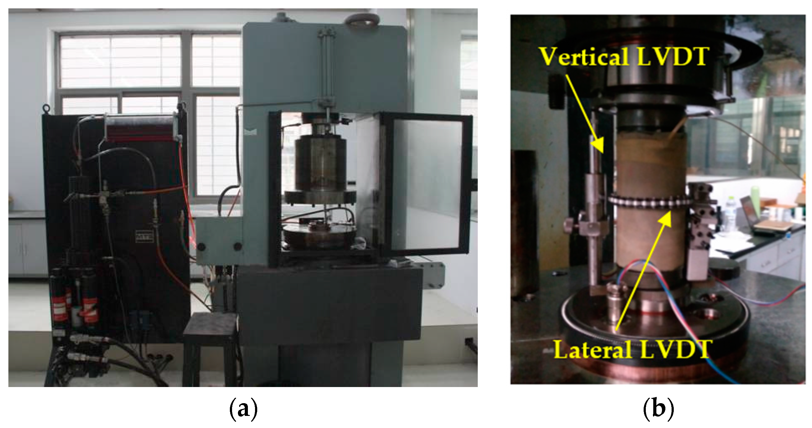
2.2. Experimental Setup

Cyclic uniaxial and triaxial compressive experiments were carried out on the shale specimens in an MTS815.03 test machine (Figure 3a) in Institute of Rock and Soil Mechanics, Chinese Academy of Sciences in Wuhan, China. This is a servo-controlled experimental system and the frame of the machine has a stiffness of 11 GN/m. The system can provide a maximum axial loading of 4600 kN and confining pressure as high as 140 MPa.
In this study, we use a thin layer of Vaseline between the sample and platen to decrease the end effect. A pair of Linear variable differential transformer (LVDT) was used to measure the vertical and lateral strain of the specimens during the whole process of the cyclic experiments (Figure 3b). It should be noted that the lateral LVDT is usually installed in the middle part of the sample, but actually the lateral strain may vary along the direction of height. Some differences of the lateral strain are owing to end effect, which may limit the lateral deformation of the samples near the two ends. The use of Vaseline can decrease this effect.

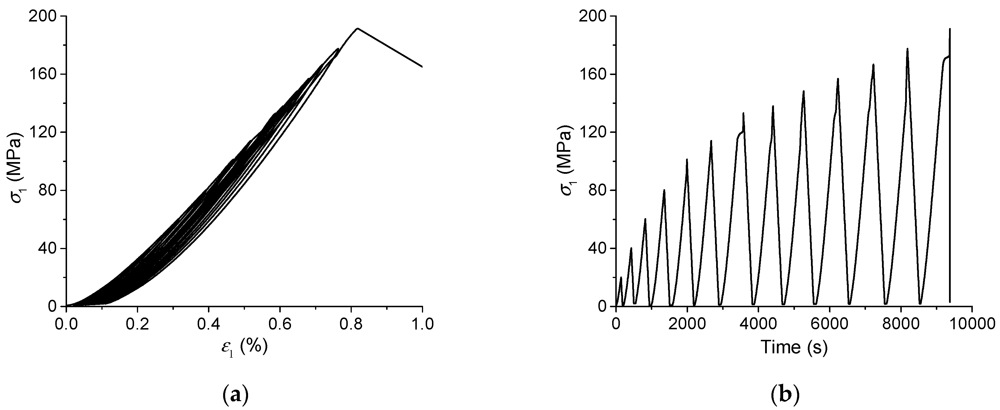
2.3. Experimental Method

For the tests on the samples with each inclination angle, various isostatic pressures (0, 20, 40, 60, and 100 MPa) were added firstly, thereafter the axial stress was given at a constant axial strain rate of 1.0 × 10⁻⁵ s−1. There are a series of cycles of loading and unloading before the peak strength. Axial unloading was applied when the pre-set axial stresses were reached with an unloading rate of 0.5–1.0 MPa/s, while keeping the confining pressures constant. The maximum axial load of each cycle will be increased to a higher value than that of the former cycle. As the tests on the samples with different inclination angles and confining pressures show quite different peak strengths, there are also different numbers of cycles for each of the tests. Take the experiment on the sample with β = 30° under uniaxial compression (σ3 = 0 MPa) as an example, Figure 4 presents the axial stress–strain axial stress–time curves to show the cycles of loading and unloading. It should be noted that for the samples with inclination angle β = 30°, only three different confining pressures (σ3 = 0, 20, and 60 MPa) were considered successfully in the experiments.

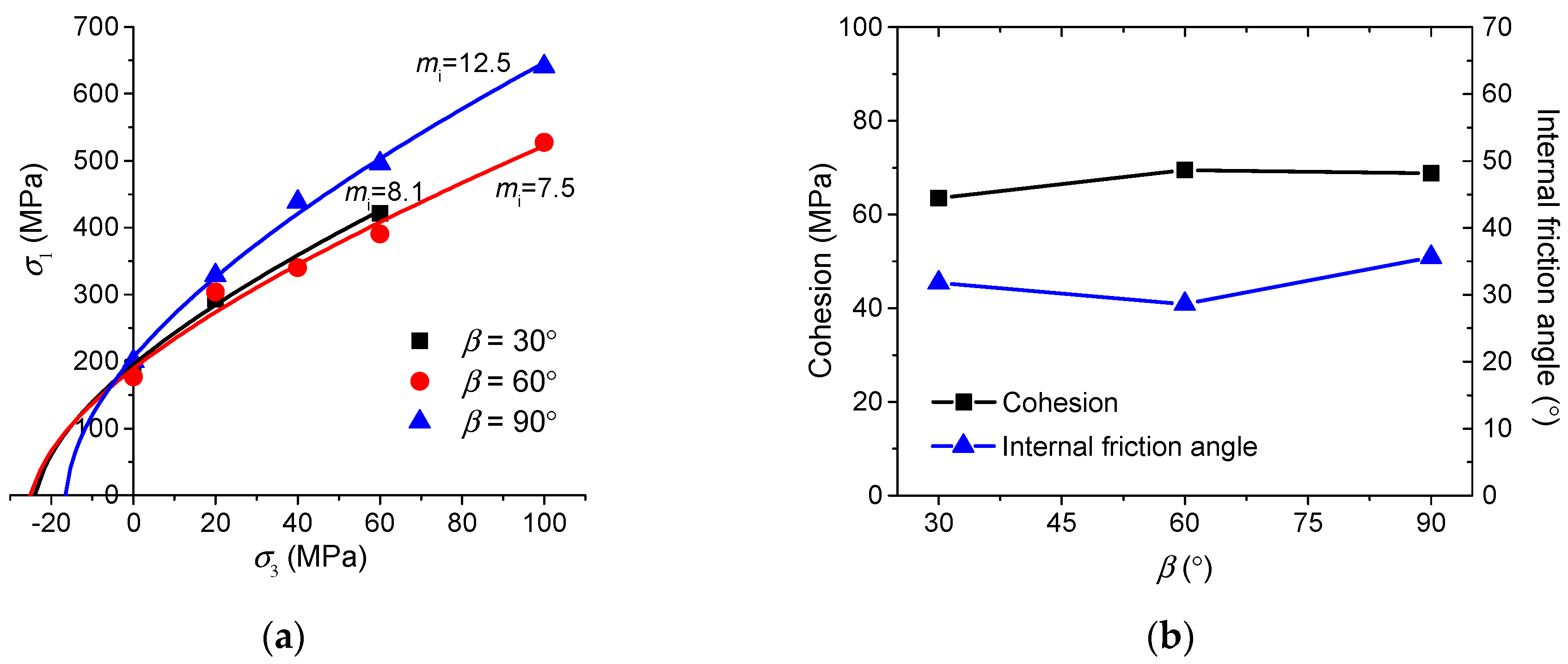
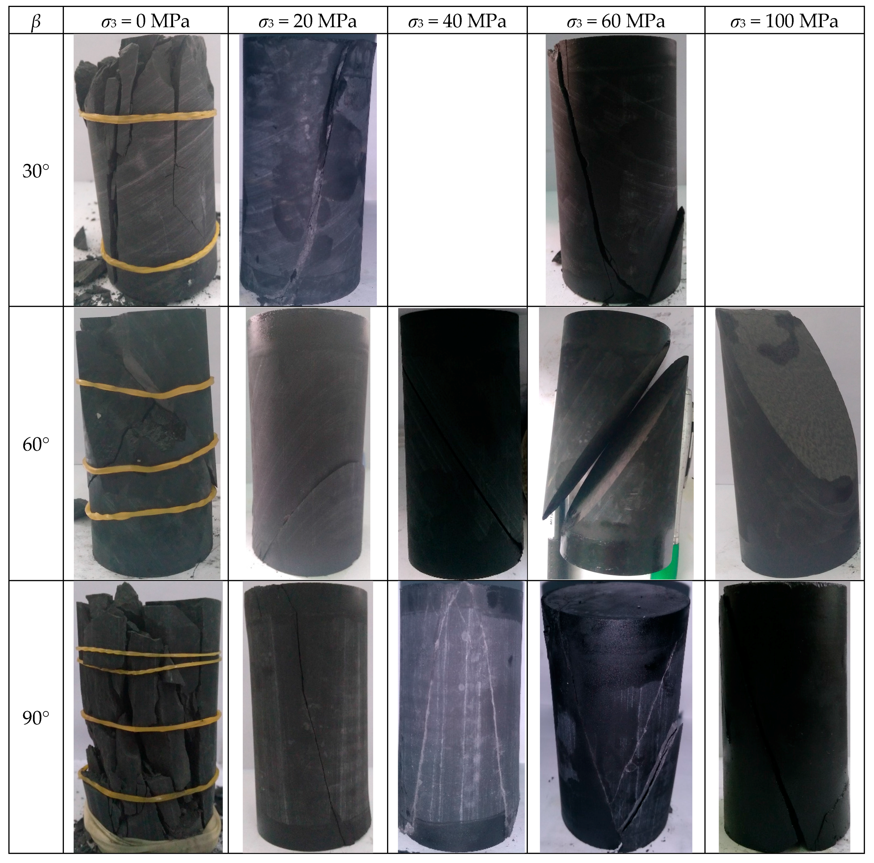
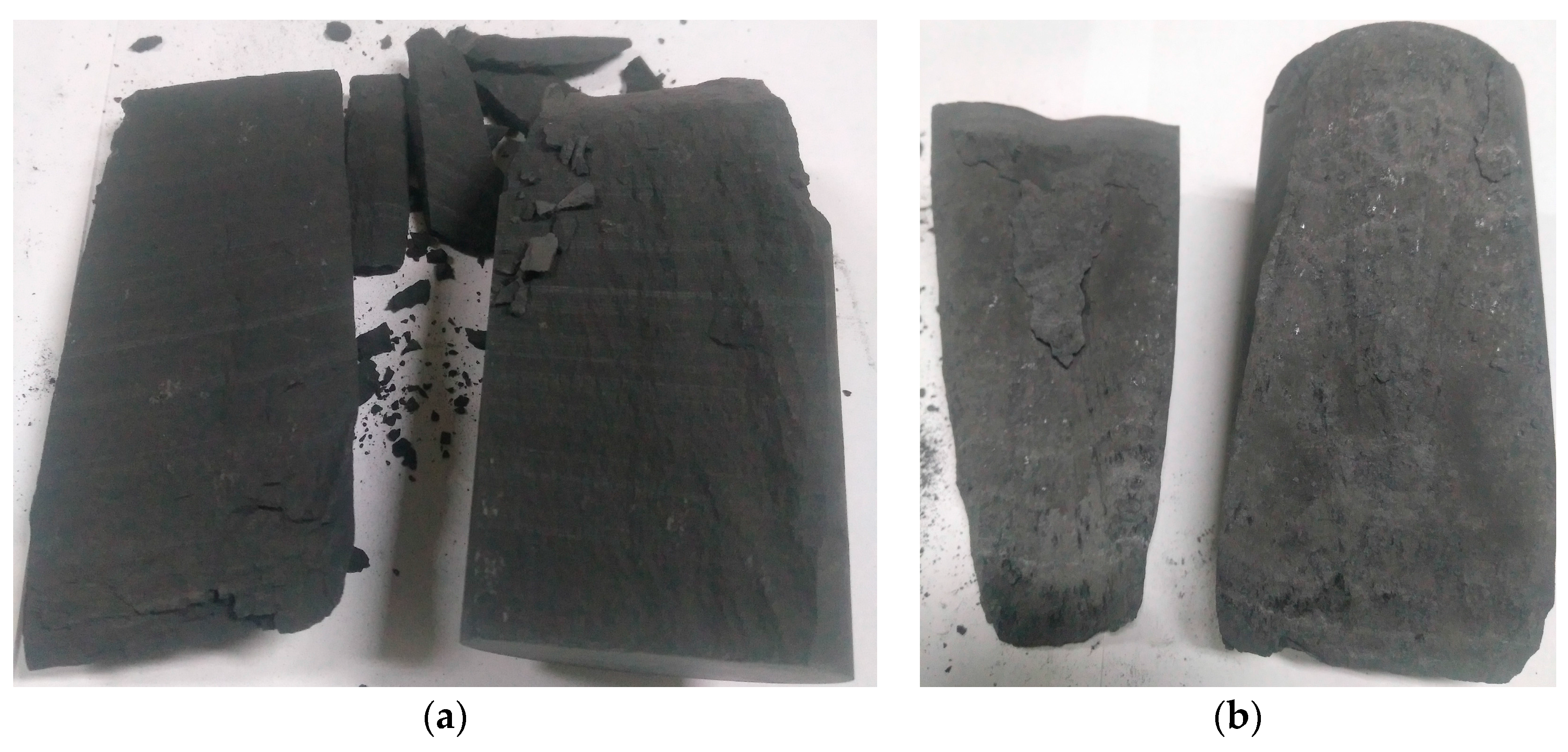
3. Experimental Results: Strength Properties and Failure Patterns

The values of peak strength and peak strain obtained from these tests are presented in Table 2. Based on the peak strength values plotted in Figure 5a, and Hoek-Brown strength criterion is used to fit the test results for the samples with different inclination orientations. Hoek-Brown strength criterion for the intact rock [40] is:
σ 1 = σ 3 + σ c ( m i σ 3 σ c + 1 ) 0.5 ,
where σ1 and σ3 are the maximum and minimum principal stresses, respectively, mi is a material parameter, and σc is the uniaxial compressive strength of the intact rock. It can be shown that the samples with β = 60° have the lowest peak strength under various confinements, and the value of mi is also lower when comparing with the other cases. The samples with β = 90° have the highest peak strengths and the mi value is also a little higher.
Mohr-Coulomb strength criterion is also applied for studying the cohesion and internal friction angle of the samples with different inclination angles. It is interesting to find from the results in Figure 5b that the samples with β = 60° have the highest cohesion, while lowest internal friction angle. This is different from some other shale specimens [8]. It has been studied that the weak planes of the shale specimens has quite high cohesion ( c w = 68.7 MPa) and a relatively low friction angle ( ϕ w = 28.8°) [41]. It is believed that these mechanical properties of the weak planes play an important role in the cohesion and internal friction angle of the specimens with different inclination angles.
The failure patterns are plotted in Figure 6. For the samples with β = 30°, vertical extension fractures can be observed clearly crossing the weak planes under the uniaxial test, and shear fractures occur in the shale matrix with the increasing of confinements; For the samples with β = 60°, both slip along the weak planes and fractures in the shale matrix can be shown under the uniaxial test, while only slip along the weak planes happen as the confining pressures increases. For the samples with β = 90°, the sample is almost totally failed by the vertical fractures under the uniaxial test, while the shear fractures dominate the failure of the samples under higher confining pressures.
The fracturing surfaces of sample S30-0 and S30-60 are presented in Figure 7 as examples to illustrate the distinctions between the tensile and shear fractures. Sample S30-0 (β = 30° and σ3 = 0 MPa) show the typical extension failure surfaces where the original tomography of the fractures can be observed clearly without any slippage or scratch, and the layers of weak planes can also be seen obviously. For sample S30-60 (β = 30° and σ3 = 60 MPa), the shear fracturing surfaces are seriously scratched by the slippage between the fractured blocks, and the weak planes cannot be found any more.

4. Evolutionary Behaviors of Strain Energy during the Tests
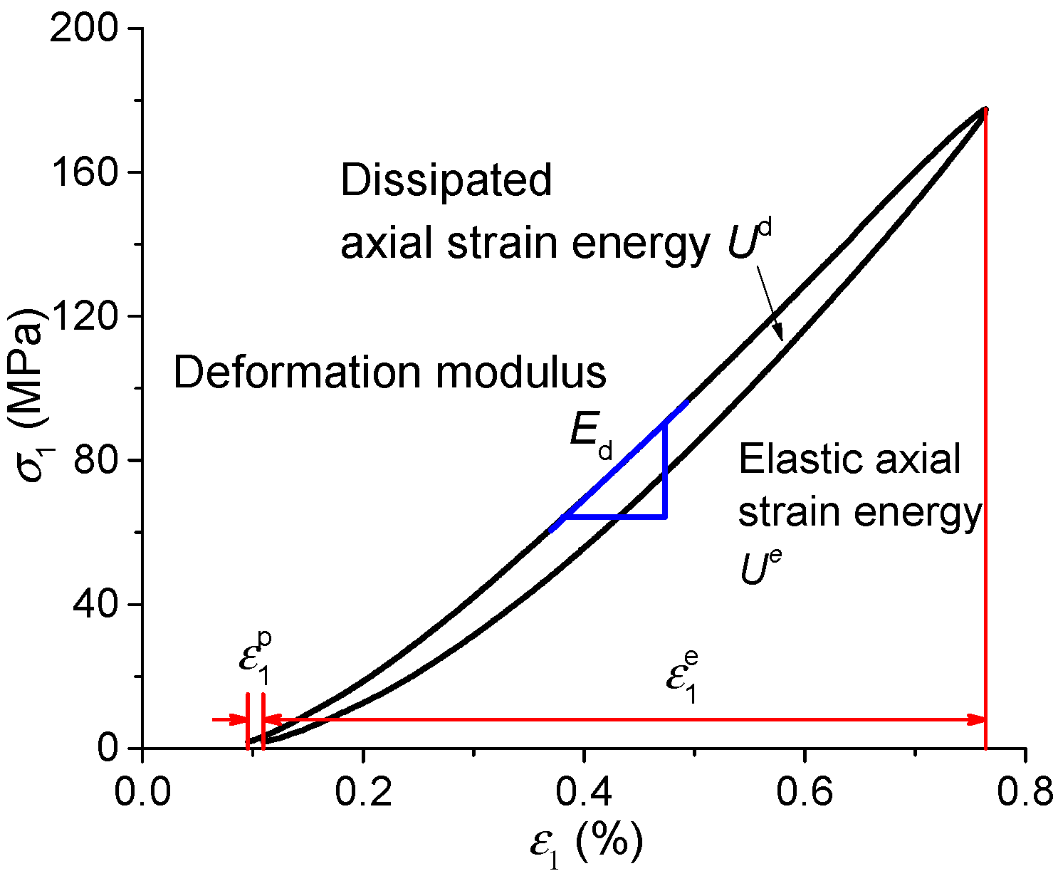
4.1. Definitions

With the cyclic loading and unloading, the energy evolution and deformation behaviors can be analyzed during the damage process for the shale specimens with different oriented weak planes and confining pressures. It should be noted that only pre-peak damage process is considered in this study, as the shale samples are so brittle that it is hard to obtain the post-peak stress-strain curves, unless the confining pressure is very high. Figure 8 presents the related parameters with a cycle of axial stress-strain curve from the test on sample S30-0 shown in Figure 4a, and they are defined in the following paragraphs.
The work done by the vertical loading and confining pressures during the whole experimental process transfer to various types of energy, including the strain energy and thermal, acoustic, magnetic energy, etc. Usually, strain energy takes the highest percentage in all of the energy types. The total strain energy U is always composed of the releasable elastic strain energy Ue and the dissipated strain energy Ud:
U = U e + U d ,
The total strain energy U and the releasable elastic strain energy Ue can be calculated according to the following equations:
U = 0 ε 1 σ 1 d ε 1 + 0 ε 2 σ 2 d ε 2 + 0 ε 3 σ 3 d ε 3 ,
U e = 1 2 σ 1 ε 1 e + 1 2 σ 2 ε 2 e + 1 2 σ 3 ε 3 e
where, σ1 and ε1 are the axial stress and axial strain, respectively. In the uniaxial compression and convention triaxial compression tests, the lateral stress σ2 = σ3 and the lateral strain ε2 = ε3, and they are written as σ3 and ε3 in the following sections. It should be noted that usually the unloading curve cannot be obtained when the peak stress is reached. It is assumed that the ratio of Ud/U in the cycle of peak stress is the same with that in the previous cycle. With this assumption, the elastic and dissipated strain energy in the cycle of peak stress can be estimated reasonably.
In addition, the Young’s modulus may also have some variations for each cycle during the damage process. As Young’s modulus is defined under the uniaxial condition, the name of deformation modulus is used in this study to consider the cases with different confining pressures. In this study, the slope of the elastic portion of the loading stress-strain curve for each cycle is calculated as the deformation modulus Ed:
E d = d σ 1 d ε 1 ,
It should be noted that the axial strain and lateral strain include elastic and plastic portions, as the following equations:
ε 1 = ε 1 e + ε 1 p , ε 3 = ε 3 e + ε 3 p
The deformation modulus and plastic strain may also be useful for evaluating the damage behavior of the shale samples, and the related information will be provided in the Appendix A. It should also be noted that the lateral strain is measured in the middle part of each sample. In the future studies, distributed optical fiber sensors may provide a better method to measure more lateral strain values at different parts of the specimens. With the development of high energy CT scanning during the experimental process, more detailed information of both vertical and lateral strain field may also be obtained. The plastic strain is also applied in this work to study its behaviors during the damage process.

4.2. Energy Evolution Behaviors during the Damage Process

Dissipated strain energy Ud has been calculated according to the cycles of loading-unloading curves for each of the tests. Strain energy dissipation behaviors with increasing axial stress are shown in Figure 9 and Figure 10 when considering both the loading directions and confining pressures. Generally speaking, strain energy dissipation increases with the axial stress increasing to the peak strength for each of the tests in this study.
Influence of confining pressures on strain energy dissipation can be analyzed according to Figure 9, for the samples with each of the inclination angles (β = 30°, β = 60°, and β = 90°). Under uniaxial compression (σ3 = 0 MPa), dissipated strain energy Ud increases gradually as the axial loading increases, and there is not a significant growing of Ud when the peak strength is approaching. However, with the increase of confining pressures, the curves of the Ud show different changing trends, i.e., the strain energy dissipation Ud is quite low at the beginning process of the axial loading, thereafter it turns to increase much more significantly until the reach of peak strength. When comparing with the fracturing patterns shown in Figure 6, extension fractures occur under uniaxial compression with lower dissipation of strain energy, while much more strain energy is dissipated for the coalescence of the cracks and formation of shear fractures, as well as the friction on the fracture surfaces under higher confining pressures.
It is also observed that the samples with different inclination angles of weak planes show different behaviors of strain energy dissipation Ud based on Figure 10. Under uniaxial compression, the curves of Ud for the samples with different oriented weak planes are very close, as the cohesion of weak planes are very high and the extension fractures are very obvious in the shale matrix for the specimens with all of the inclination angles (Figure 6). With increasing confining pressures, the growing of the strain energy dissipation show different trends. For the shale sample (β = 60°), the increase of strain energy dissipation is obviously slower than the other two conditions, because the fracturing is mainly slip along the weak planes (Figure 6), and it is not required to dissipate to much strain energy to form the shear plane because the friction angle of the weak planes is quite low ( ϕ w = 28.8°). It should also be noted that the strain energy dissipation increases more significantly for the samples (β = 30°) than the specimens (β = 90°), this may be related to the observations that the shear fractures have larger angles with the weak planes in the samples (β = 30°), and the fractures may need more energy to cross these weak planes.
The ratio of the releasable elastic strain energy Ue to the dissipated strain energy Ud has been defined as the burst proneness index, and the higher ratio of Ue/Ud indicates a higher probability of rock burst [42]. This ratio is also related to the brittleness index Ue/U, and the higher ratio means that the rock material is more brittle [43]. Consequently, the ratio Ue/Ud is a very useful parameter to estimate the stability of wellbore or the brittleness of the shale reservoir.
The ratios that were obtained from all conditions of the tests are plotted in Figure 11. Generally speaking, for most of the tests, the ratio increases at first with the increasing axial loading, then decreases when the peak strength is approaching. The ratio is lower at the beginning of loading as some energy is dissipated during the crack closure process. At the elastic and stable crack propagation processes, less dissipation of strain energy leads to the higher value of the ratio. When the peak strength is approaching, the ratio decreases again as more strain energy is dissipated with the unstable crack propagation and friction on the fracture surfaces. It is also observed that the change of this ratio is not very obvious for the tests under uniaxial compression, as the formation of extension fractures need lower strain energy than the coalescence of shear fractures under higher confining pressures. The ratios obtained in the cycle of peak stress are plotted in Figure 11d. The general decreasing trend of the samples show the reduction of brittleness with increasing confining pressures. The samples (β = 60°) have the highest ratio under various confinements, showing that the shale samples are more brittle under this loading direction.

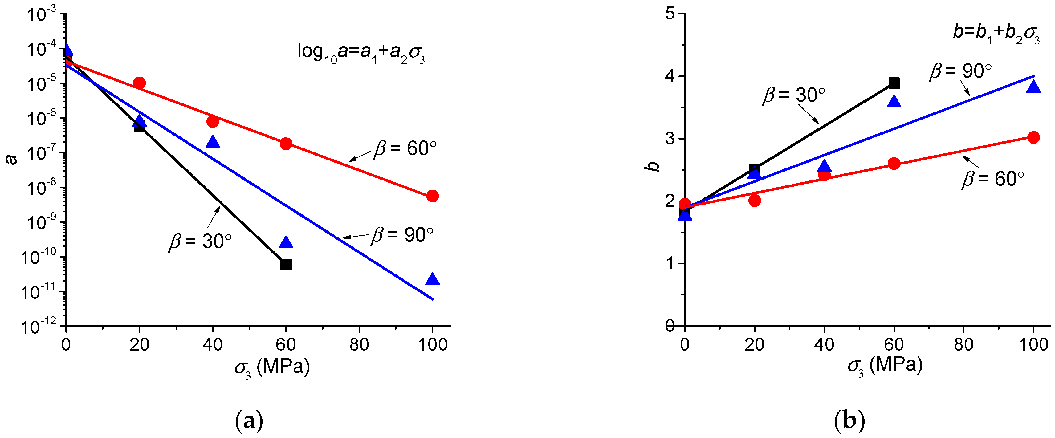
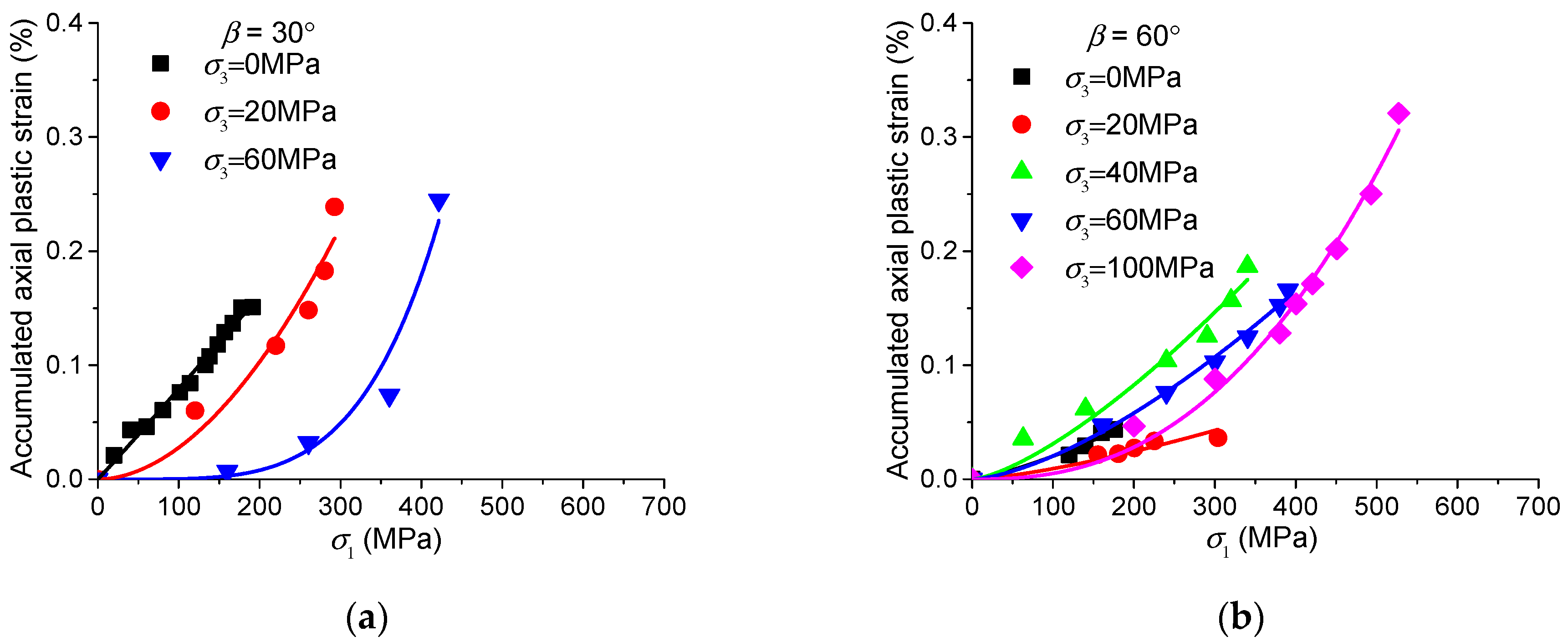
5. Damage Variable and Damage Evolution Equation

5.1. Definition of the Damage Variable

Damage variable is usually defined to quantifying the evolutionary damage process, and a well-defined damage variable can be connected to the loading/unloading process to build the damage evolution equation. Based on the analyses in the last section, the evolution of strain energy dissipation is closely related to the failure process of the shale samples, and can be used to estimate the damage degree of the shale. The dissipated strain energy has been used to define the damage variable in the previous studies [22,44]. Here, in this study, the dissipated strain energy in each cycle during the pre-peak loading ( U i d ) normalized by the dissipated strain energy at peak stress ( U f d ) are considered as the damage variable D:
D = U i d U f d ,
This damage variable can be used to describe the damage state of a representative volume element (REV) of the rock material. It is assumed that there is no damage in the REV before the axial loading is applied (D = 0). With the increase of axial loading, the dissipated strain energy increases and the REV is gradually damaged until D = 1 when the peak strength is reached.
With this definition, we can study the damage evolution of the shale samples during the pre-peak loading process when considering both loading directions and confining pressures.

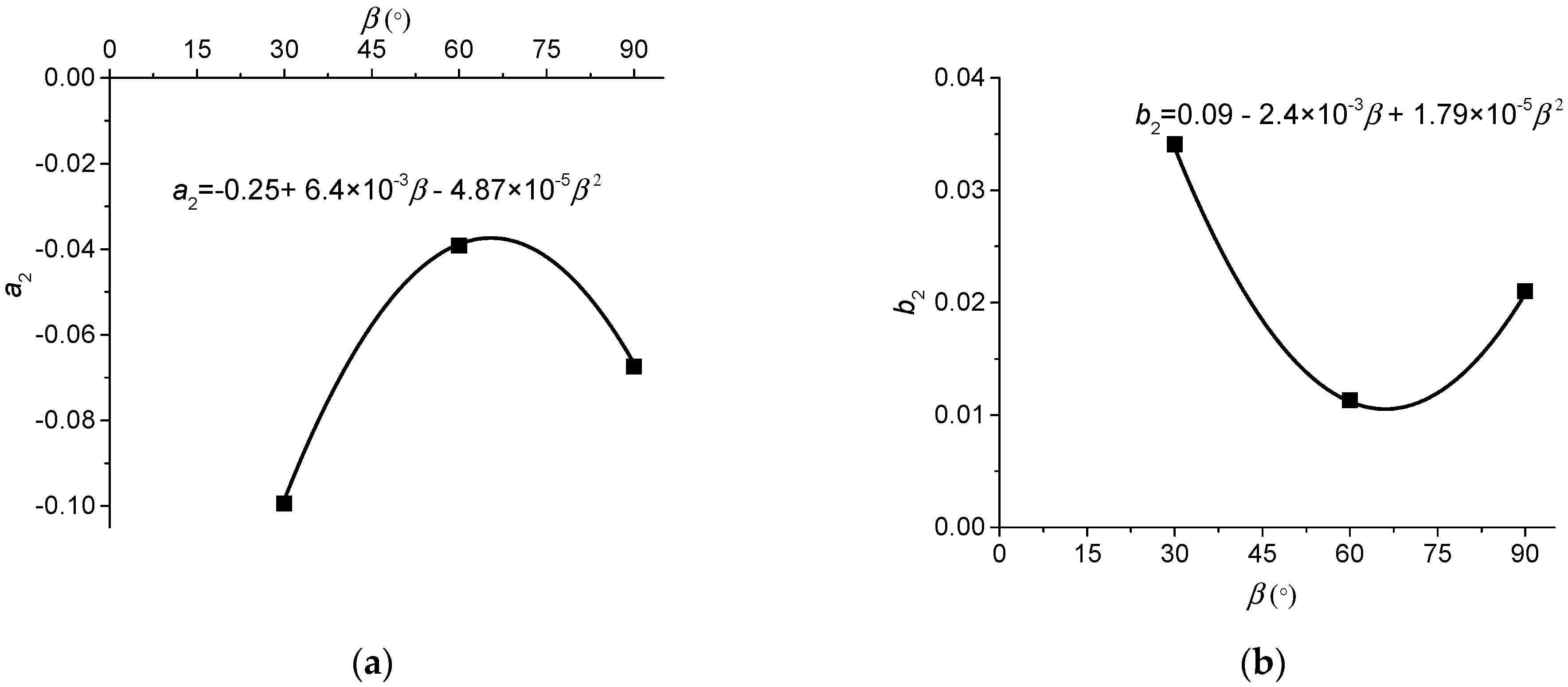
5.2. Damage Evolution Equation

The evolution of the damage variable D is plotted in Figure 12 with the increase of axial stress σ1. Power function can be used to fit the damage evolution equation:
D = a σ 1 b ,
where a and b are two constant parameters. The data of damage variable D are well fitted (Figure 12), and the fitted parameters are presented in Table 3. This equation build the damage variable and the axial loading conditions. As defined in Section 5.1, the damage variable D indicates the degree of damage based on the dissipated strain energy, therefore Equation (8) can describe the evolutionary damage process with the increase of axial loading.
Apparently, constant parameters a and b can significantly affect the curvature of the D-σ1 curves based on damage evolution Equation (8). In fact, this is caused by the variation of inclination angle β and confining pressures σ3. According to the fitted D-σ1 curves presented in Figure 12, for the samples with all the three different inclination angles β, the damage variable D increases at a relatively similar rate during the axial loading process under uniaxial compression (σ3 = 0 MPa). With the increasing confining pressures, the damage variable D turns to increase very slowly at the beginning of loading, followed by a significant increase when the peak strength is approaching. This is reasonable when comparing with the damage process of the shale samples. Under uniaxial compression (σ3 = 0 MPa), the damage process usually includes the crack initiation, propagation, coalescence, and formation of the macro tensile fractures. With increasing confining pressures, the crack initiation and propagation is to some extent limited by the confinements at the early stage of axial loading, however, the formation of shear surface, as well as the slippage along the surfaces occurs when the axial stress is approaching the peak strength, leading to a significant increase of damage variable D.
The influence of inclination angel on the damage evolution can be observed according to the curves presented in Figure 13. Under uniaxial compression (σ3 = 0 MPa), the D-σ1 curves are almost the same for the samples with different inclination angles. Under higher confining pressures, the D-σ1 curves begin to show some different characteristics: for the sample with inclination angle β = 60°, the increasing rate of damage variable D has weaker changes during the loading process when compared with the cases of β = 30° and 90°. These are also reasonable when comparing with the cracking and fracturing process of the samples. When σ3 = 0 MPa, the formation of fractures by splitting the rock material occurs in each of the samples with different inclination angles. With increasing confining pressures, the cracking and fracturing process of the shale sample with β = 60° occurs gradually along the weak planes, while for the samples with β = 30° and 90°, the crack initiation and propagation occurs slowly at the early stage of compression and the formation of macro shear fractures lead to a significant increase of damage when the axial stress approaches the peak strength.
Consequently, the damage evolution Equation (8) can reflect the damage process of shale samples when considering both the inclination angle and confining pressures. The relationship between the constant parameters (a and b) and the two factors (β and σ3) can be discussed as follows:
Firstly, for the samples with each of the inclination angles, the parameters a and b are dependent on the confining pressures σ3. With the values of a and b plotted in Figure 14, it can be found that the relation between these two parameters and σ3 can be further fitted by the following equations:
log 10 a = a 1 + a 2 σ 3 ,
b = b 1 + b 2 σ 3 ,
where a1, a2 and b1, b2 are also constant parameters, and their fitted values are shown in Table 4. In this way, the damage evolution equation with the increasing σ1 can be built dependent on the confining pressure σ3 for the shale samples with different oriented weak planes.
Secondly, these parameters can be further fitted with the inclination angle β. According to Figure 14 and Table 4, it can be found that the parameters a1 and b1 remain almost constant for the cases of different inclination angles β. Therefore, it is only required to build relationship between the parameters (a2 and b2) and β. Based on the different values presented in Table 4, the relationship can be fitted as shown in Figure 15. It should be noted that this relationship is only suitable for the cases of 30° ≤ β ≤ 90°, and systematic experiments on the samples with more different inclination angles should be carried out to make the equations more reasonable and reliable.
In this section, the damage evolution equation is built based on the evolution of strain energy dissipation, which has been proved to be closely related to the crack propagation and fracturing of the rock material. It can be used to describe the damage process of the shale samples with different oriented weak planes and confining pressures during the pre-peak loading. Based on this damage evolution equation, constitutive relationship can be studied for the shale samples when considering different loading directions and confining pressures; therefore, it is helpful for understanding the wellbore stability in the shale reservoir.

6. Conclusions

Based on a series of cyclic uniaxial and triaxial compressive experiments on the shale samples with different oriented weak planes and confining pressures, the damage behaviors are researched during the pre-peak loading process. The main findings are as follows:
(1)
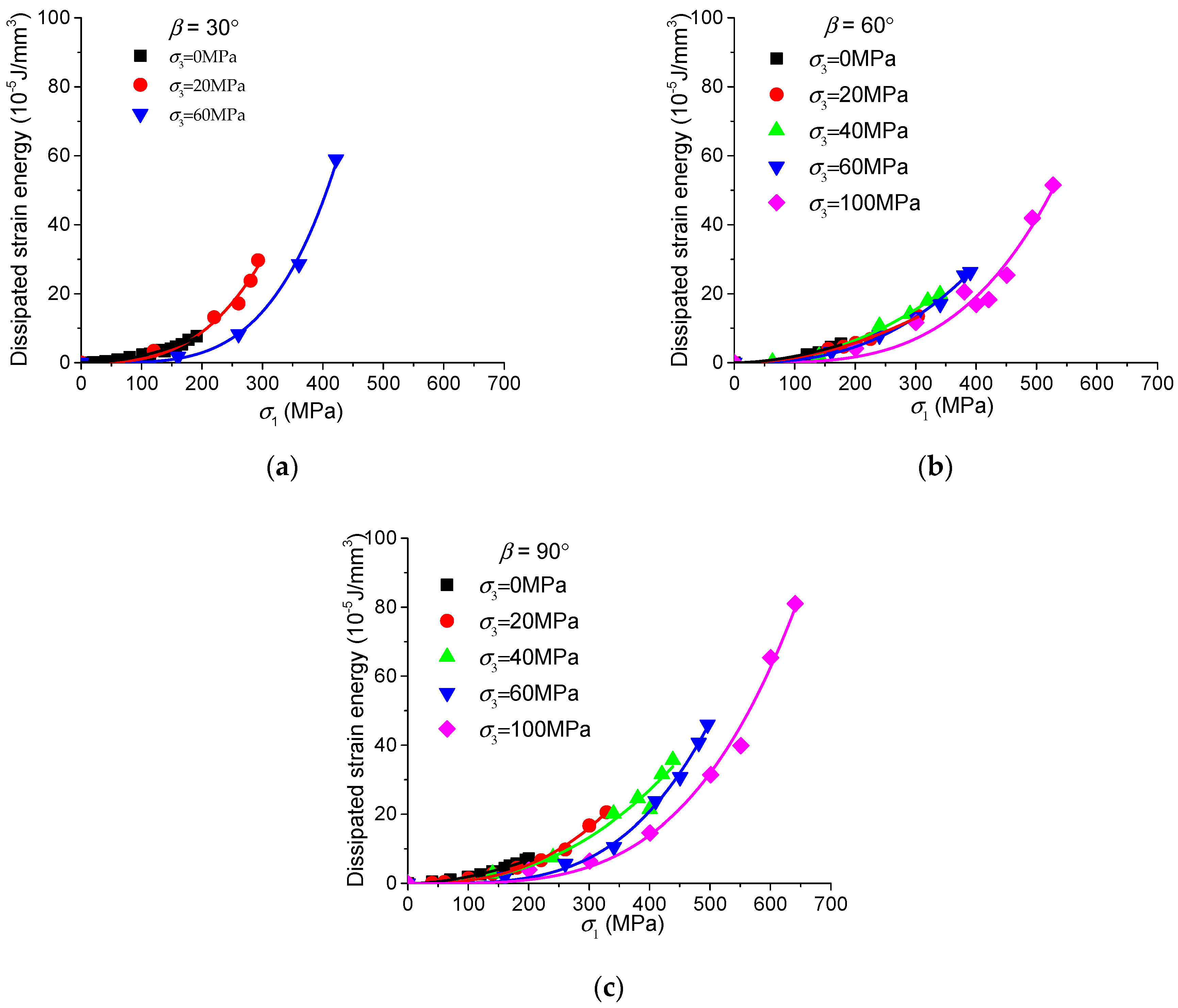
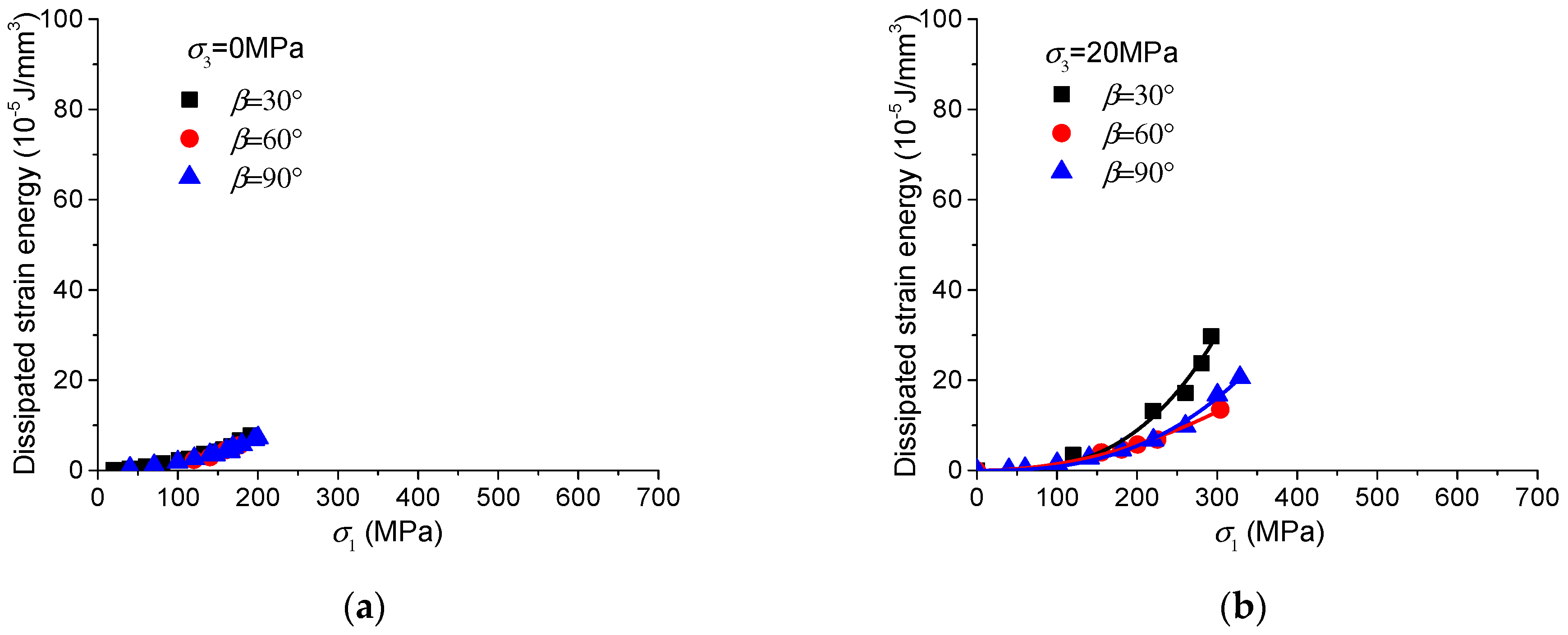
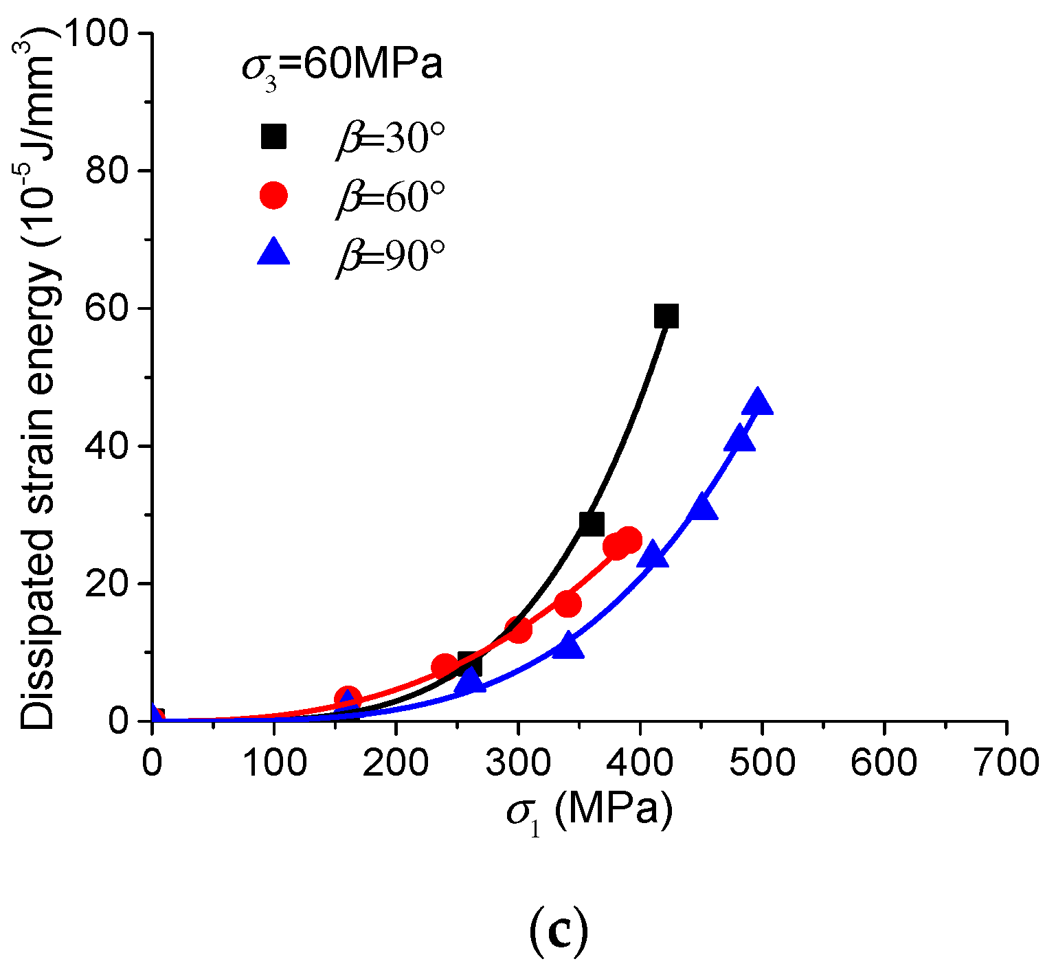
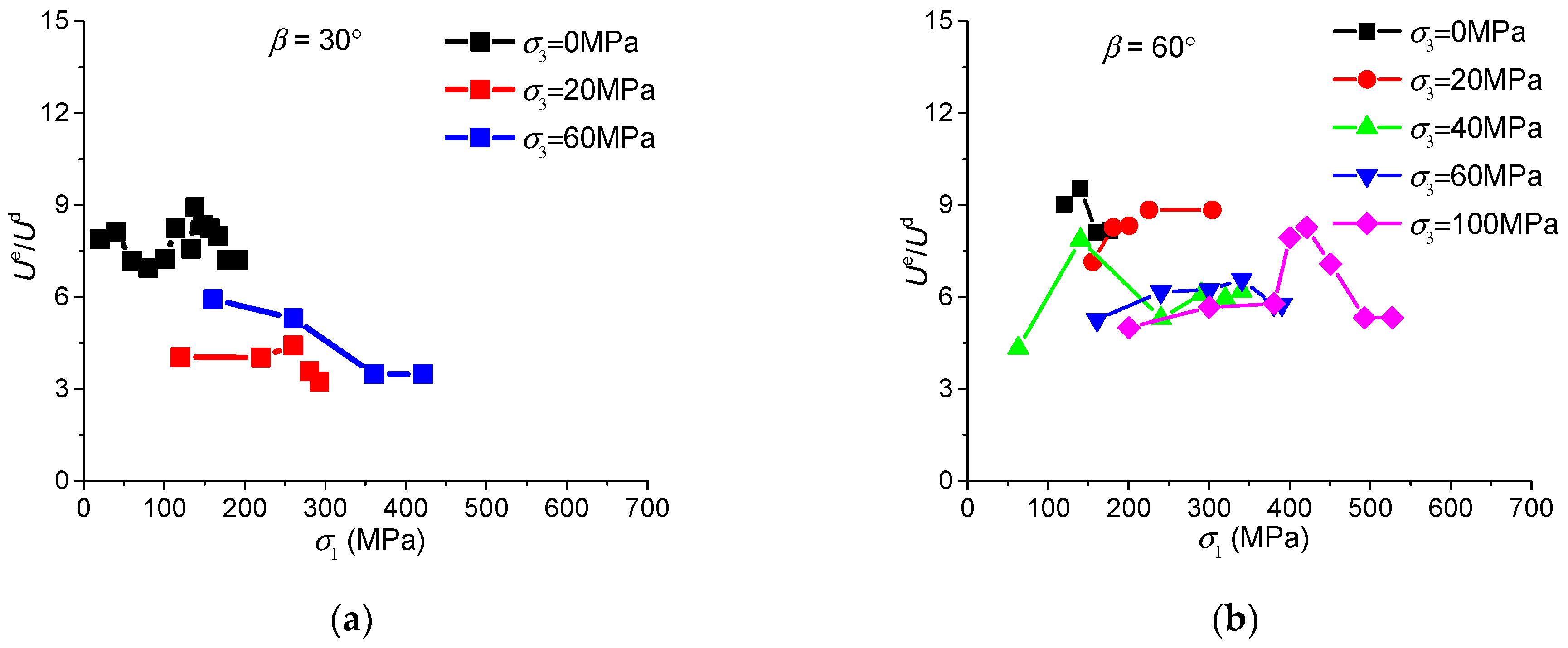
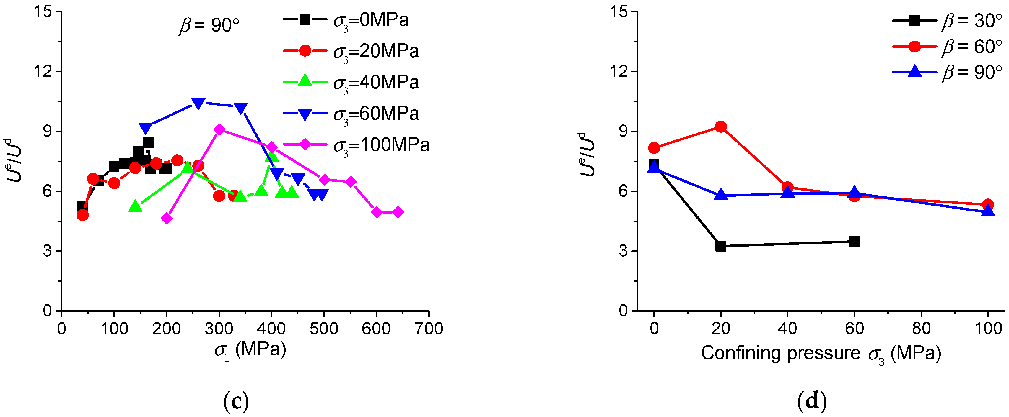
The evolution characteristics of the strain energy dissipation are observed for the shale samples with different oriented weak planes under different confining pressures. Under uniaxial test, the strain energy dissipation increases slowly with the increasing axial loading; under higher confining pressures, the strain energy dissipation increases slowly at the beginning process of axial loading, while there is a significant increase when the peak stress is approaching. For the shale samples with inclination angle β = 60°, the increase of the strain energy dissipation is not so significant as the cases of β = 30° and 90°.
(2)
These behaviors of strain energy dissipation are closely related to the different fracturing patterns of the samples under different loading directions and confining pressures. Generally speaking, the formation of extension fractures dissipates less strain energy, while the coalescence of shear fractures and the friction on the fracture surfaces dissipate much more strain energy. For the slip along the weak planes with a low friction angle, the dissipated strain energy is also limited. The different characteristics of strain energy dissipation are related to the corresponding fracturing patterns.
(3)
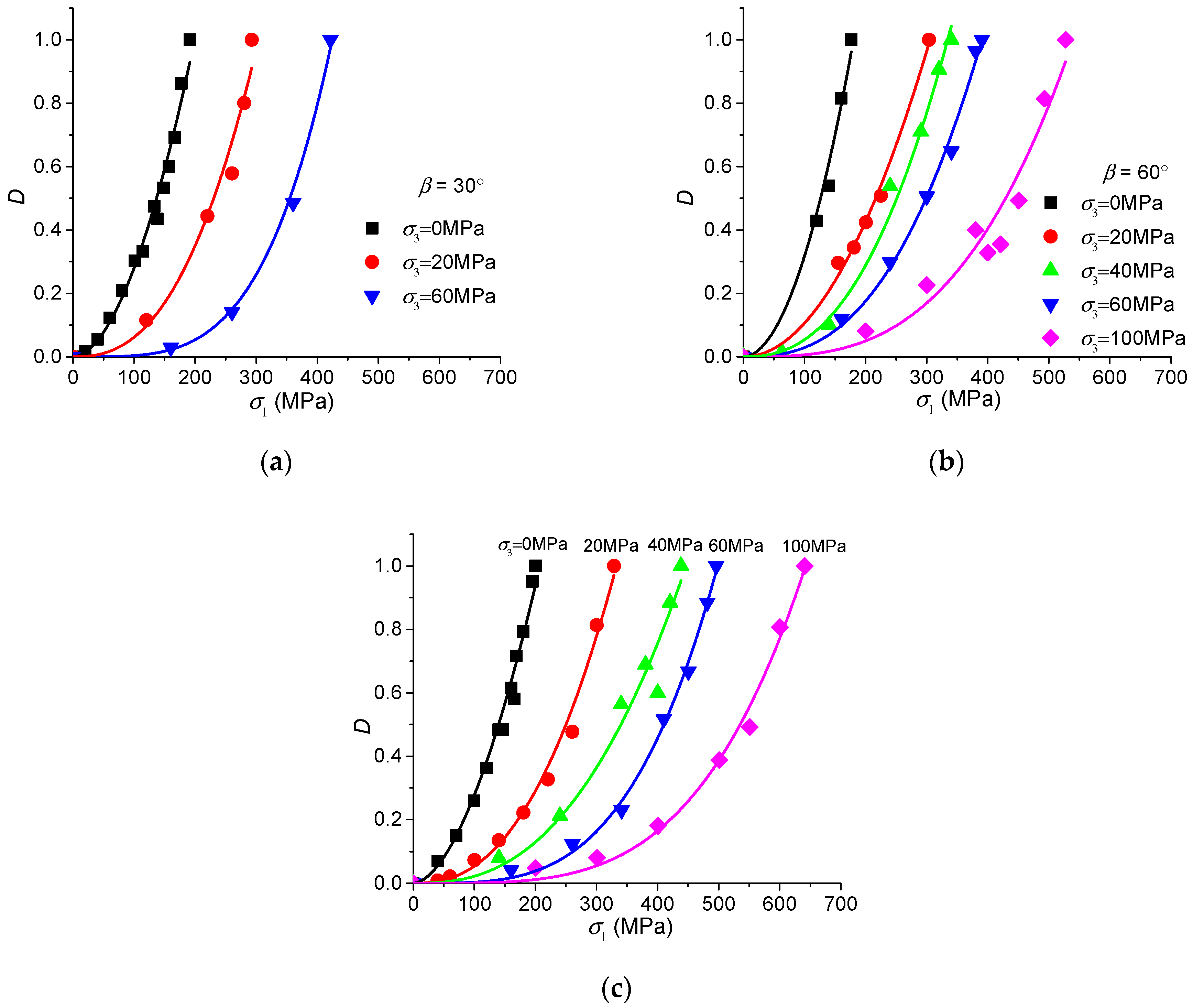
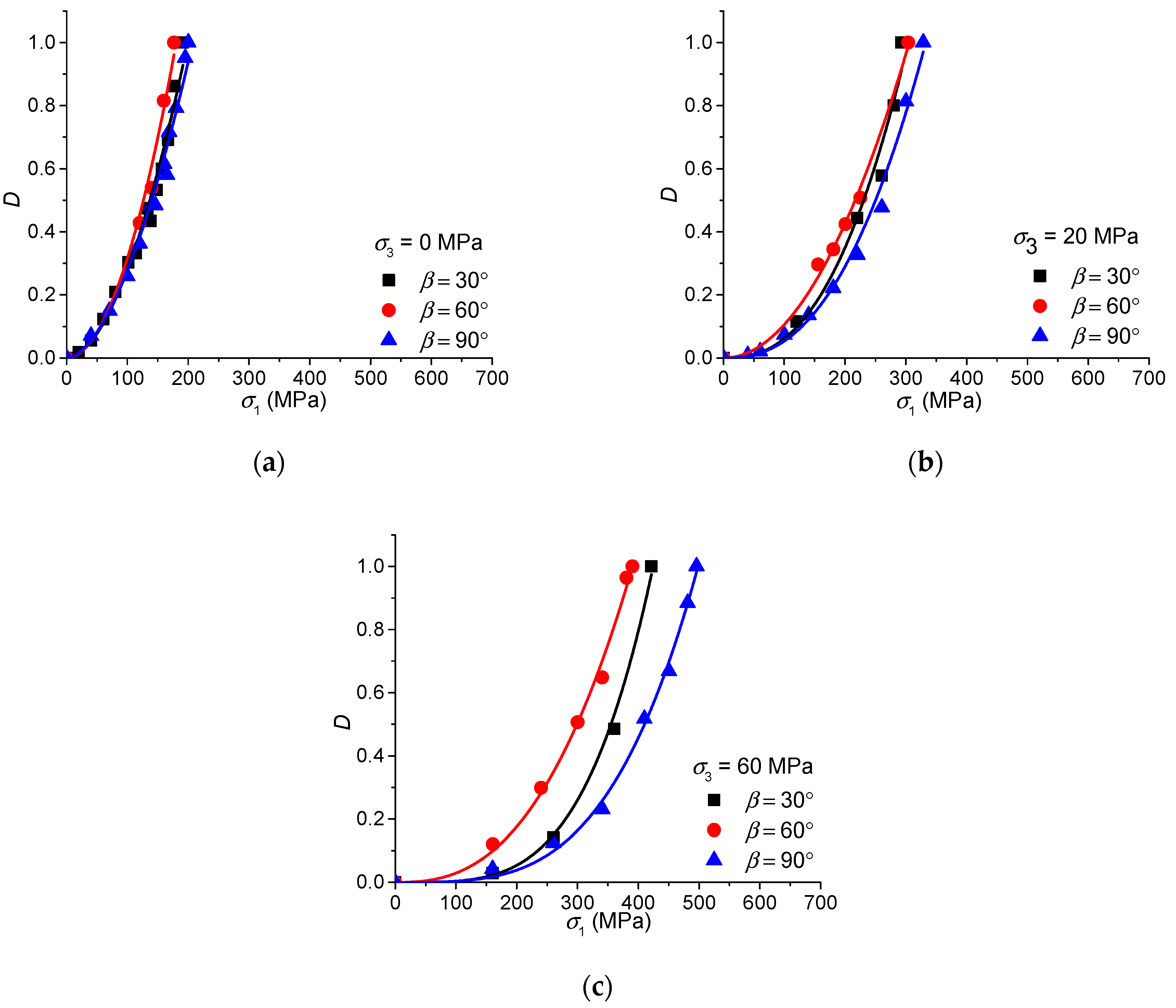
The damage evolution equation is built dependent on the loading directions and confining pressures. The damage equation shows that the damage of the shale samples increases as a power function of the axial stress. This damage evolution equation can be used for describing the damage process of the shale samples, and it can also be helpful for build constitutive equations of the shale when considering both the orientation of weak planes and various stress states.
This study is helpful for understanding the deformation and failure of wellbore, as well as the effect of stimulation in the shale gas reservoir. The mechanical behaviors obtained from the cyclic uniaxial and triaxial experiments can also provide a database for further analyzing the damage behaviors of different shale samples. The damage evolution equation can be used for building constitutive equations and modeling the shale samples. It should also be noted that this work only analyzed the pre-peak damage process, and the post-peak failure is also important for the shale in the oil and gas engineering, and it will be studied in the future work based on the cyclic uniaxial and triaxial tests in this study also for the modelling of damage behaviors of shale in the future work.

Acknowledgments

This work is financially supported by the Strategic Priority Research Program of the Chinese Academy of Sciences (No. XDB10050201 and XDB10030301), and National Natural Science Foundation of China (No. 41402286). Hua Zhang from Institute of Rock and Soil Mechanics, CAS is acknowledged for his help in the laboratory experiments. The anonymous reviewers gave very helpful suggestions, which were valuable for improving our manuscript.

Author Contributions

Cheng Cheng designed and conducted the laboratory experiments, made the analyses and wrote the paper; Xiao Li designed the framework of the research and guided the analyses.

Conflicts of Interest

The authors declare no conflict of interest.

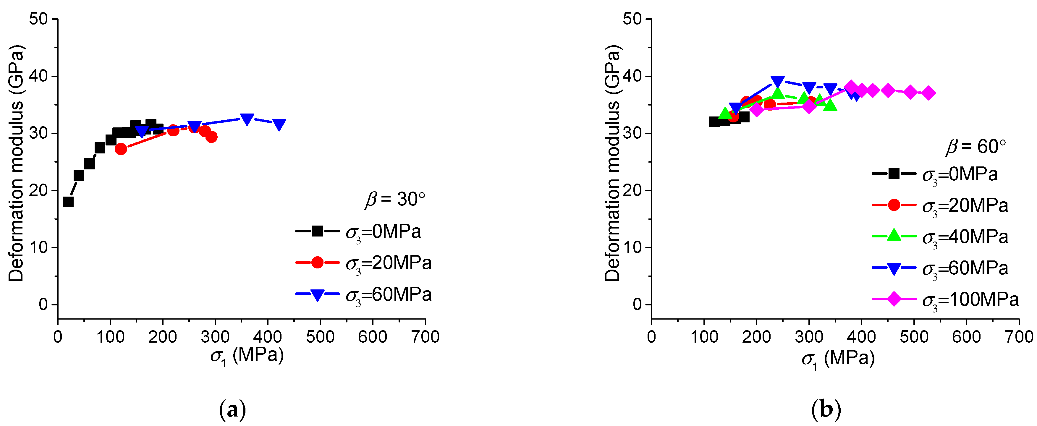
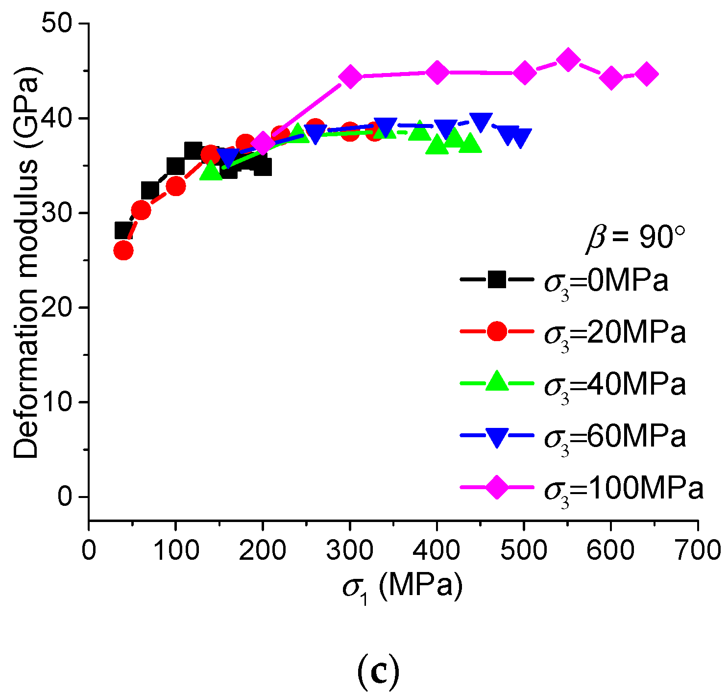
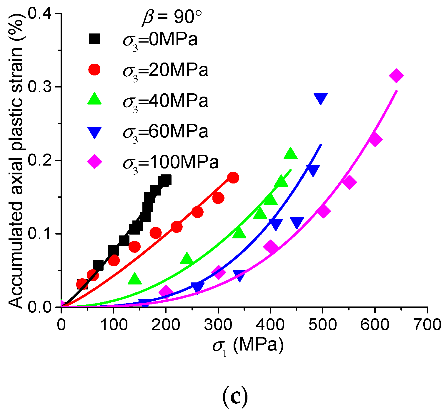
Appendix A. Deformation Behaviors during the Damage Process

(1) Deformation modulus
Variation of deformation modulus with increasing axial loading can be observed in Figure A1. Generally speaking, deformation modulus increases at the beginning of loading owing to the closure of pre-existing cracks. Thereafter, the deformation modulus keeps almost constant and only a little reduction occurs when the peak strength is approaching. The samples (β = 30°) have the lowest deformation moduli because the axial loading has quite a large angle with the weak planes, and the samples (β = 90°) have the highest deformation moduli because the axial loading is parallel with the weak planes. With increasing confinement, there is a general increase of deformation moduli for the samples with different oriented weak planes. However, the increase of deformation moduli is less obvious for the samples (β = 30°) owing to the orientation of weak planes relative to the axial loading direction.
Figure A1. Deformation modulus with the increase of axial stress for the shale samples with different oriented weak planes ((a) β = 30°, (b) β = 60°, and (c) β = 90°) under various confining pressures.
Energies 11 00160 g0a1aEnergies 11 00160 g0a1b
(2) Plastic strain
Accumulated axial plastic strain values are plotted in Figure A2. For the samples (β = 30° and 90°), the accumulated axial plastic strain increases obviously since the beginning of axial loading under uniaxial compression, without a significant increase when the peak strength is approaching. With increasing confining pressures, the accumulated axial plastic strain is very limited at the beginning of axial loading, but increases much significantly when the peak strength is reaching. For the samples (β = 60°), the accumulated axial plastic strain values are very limited during the whole process of uniaxial loading, while the values are limited at the initial loading and increase significantly with the axial stress σ1 approaches to the peak stress under higher confining pressures.
It should also be noted that the plastic strain increases almost linearly with axial stress when σ3 = 0 MPa, as there is not a very significant increase of plastic strain when the peak strength is approaching for the tensile failure of the samples. However, with the increase of confining pressures, the failure patterns turn to be shear failure, and there will be more slip when the failure plane is formed, so there is a more significant increase of plastic strain for the tests under higher confining pressures.
Figure A2. Accumulated axial plastic strain with the increase of axial stress for the shale samples with different oriented weak planes ((a) β = 30°, (b) β = 60°, and (c) β = 90°) under various confining pressures.
Energies 11 00160 g0a2aEnergies 11 00160 g0a2b

References

  1. Lian, Z.; Yu, H.; Lin, T.; Guo, J. A study on casing deformation failure during multi-stage hydraulic fracturing for the stimulated reservoir volume of horizontal shale wells. J. Nat. Gas Sci. Eng. 2015, 23, 538–546. [Google Scholar] [CrossRef]
  2. Li, Q.; Xing, H.; Liu, J.; Liu, X. A review on hydraulic fracturing of unconventional reservoir. Petroleum 2015, 1, 8–15. [Google Scholar] [CrossRef]
  3. Ma, Y.; Pan, Z.; Zhong, N.; Connell, L.D.; Down, D.I.; Lin, W.; Zhang, Y. Experimental study of anisotropic gas permeability and its relationship with fracture structure of Longmaxi Shales, Sichuan Basin, China. Fuel 2016, 180, 106–115. [Google Scholar] [CrossRef]
  4. Niandou, H.; Shao, J.; Henry, J.; Fourmaintraux, D. Laboratory investigation of the mechanical behaviour of Tournemire shale. Int. J. Rock Mech. Min. Sci. 1997, 34, 3–16. [Google Scholar] [CrossRef]
  5. Brown, S.R.; Bruhn, R.L. Fluid permeability of deformable fracture networks. J. Geophys. Res. Solid Earth 1998, 103, 2489–2500. [Google Scholar] [CrossRef]
  6. Jaeger, J.C. Shear Failure of Anistropic Rocks. Geol. Mag. 1960, 97, 65–72. [Google Scholar] [CrossRef]
  7. McLamore, R.T.; Gray, K.E. A Strength Criterion for Anisotropic Rocks Based Upon Experimental Observations. In Proceedings of the Annual Meeting of the American Institute of Mining, Metallurgical, and Petroleum Engineers, Los Angeles, CA, USA, 19–23 February 1967. [Google Scholar]
  8. Crawford, B.R.; Dedontney, N.L.; Alramahi, B.; Ottesen, S. Shear strength anisotropy in fine-grained rocks. In Proceedings of the 46th US Rock Mechanics/Geomechanics Symposium, Chicago, IL, USA, 24–27 June 2012. [Google Scholar]
  9. Fjær, E.; Nes, O.-M. The Impact of Heterogeneity on the Anisotropic Strength of an Outcrop Shale. Rock Mech. Rock Eng. 2014, 47, 1603–1611. [Google Scholar] [CrossRef]
  10. Gao, Z.; Zhao, J.; Yao, Y. A generalized anisotropic failure criterion for geomaterials. Int. J. Solids Struct. 2010, 47, 3166–3185. [Google Scholar] [CrossRef]
  11. Laloui, L.; Salager, S.; Nuth, M.; Marschall, P. Anisotropic mechanical response of a shale. In Proceedings of the EAGE Shale Workshop 2010: Shale—Resource & Challenge, Nice, France, 26–28 April 2010. [Google Scholar]
  12. Rezapour, A. Modeling of Mechanical Behaviour of Anisotropic Rocks. Master Degree Thesis, McMaster University, Hamilton, ON, Canada, 2015. [Google Scholar]
  13. Zhang, Z.; Zhang, R.; Xie, H.; Liu, J.; Were, P. Differences in the acoustic emission characteristics of rock salt compared with granite and marble during the damage evolution process. Environ. Earth Sci. 2015, 73, 6987–6999. [Google Scholar] [CrossRef]
  14. Ghamgosar, M.; Erarslan, N.; Williams, D.J. Evolution of Damage on Tensile Fracturing of Rock by Means of Elastic Ultrasonic Wave Velocity. Proceedings of Eurock, Vigo, Spain, 27–29 May 2014; pp. 297–302. [Google Scholar]
  15. Feng, X.T.; Chen, S.; Zhou, H. Real-time computerized tomography (CT) experiments on sandstone damage evolution during triaxial compression with chemical corrosion. Int. J. Rock Mech. Min. Sci. 2004, 41, 181–192. [Google Scholar] [CrossRef]
  16. Zhou, X.P.; Zhang, Y.X.; Ha, Q.L. Real-time computerized tomography (CT) experiments on limestone damage evolution during unloading. Theor. Appl. Fract. Mech. 2008, 50, 49–56. [Google Scholar] [CrossRef]
  17. Song, D.; Wang, E.; Li, Z.; Liu, J.; Xu, W. Energy dissipation of coal and rock during damage and failure process based on EMR. Int. J. Min. Sci. Technol. 2015, 25, 787–795. [Google Scholar] [CrossRef]
  18. Qiu, S.-L.; Feng, X.-T.; Xiao, J.-Q.; Zhang, C.-Q. An Experimental Study on the Pre-Peak Unloading Damage Evolution of Marble. Rock Mech. Rock Eng. 2014, 47, 401–419. [Google Scholar] [CrossRef]
  19. Martin, C.D.; Chandler, N.A. The progressive fracture of Lac du Bonnet granite. Int. J. Rock Mech. Min. Sci. Geomech. Abstr. 1994, 31, 643–659. [Google Scholar] [CrossRef]
  20. Yoshinaka, R.; Tran, T.V.; Osada, M. Non-linear, stress- and strain-dependent behavior of soft rocks under cyclic triaxial conditions. Int. J. Rock Mech. Min. Sci. 1998, 35, 941–955. [Google Scholar] [CrossRef]
  21. Li, D.; Sun, Z.; Xie, T.; Li, X.; Ranjith, P.G. Energy evolution characteristics of hard rock during triaxial failure with different loading and unloading paths. Eng. Geol. 2017, 228, 270–281. [Google Scholar] [CrossRef]
  22. Wang, P.; Xu, J.; Fang, X.; Wang, P. Energy dissipation and damage evolution analyses for the dynamic compression failure process of red-sandstone after freeze-thaw cycles. Eng. Geol. 2017, 221, 104–113. [Google Scholar] [CrossRef]
  23. Peng, R.; Ju, Y.; Wang, J.G.; Xie, H.; Gao, F.; Mao, L. Energy Dissipation and Release During Coal Failure Under Conventional Triaxial Compression. Rock Mech. Rock Eng. 2015, 48, 509–526. [Google Scholar] [CrossRef]
  24. Xie, H.P.; Li, L.Y.; Ju, Y.; Peng, R.D.; Yang, Y.M. Energy analysis for damage and catastrophic failure of rocks. Sci. China Technol. Sci. 2011, 54, 199–209. [Google Scholar] [CrossRef]
  25. Denney, D. Thirty Years of Gas-Shale Fracturing: What Have We Learned? J. Pet. Technol. 2010, 62, 88–90. [Google Scholar] [CrossRef]
  26. Jarvie, D.M.; Hill, R.J.; Ruble, T.E.; Pollastro, R.M. Unconventional shale-gas systems: The Mississippian Barnett Shale of north-central Texas as one model for thermogenic shale-gas assessment. AAPG Bull. 2007, 91, 475–499. [Google Scholar] [CrossRef]
  27. Wang, J.; Liu, Y. Simulation Based Well Performance Modeling in Haynesville Shale Reservoir. In Proceedings of the SPE Production and Operations Symposium, Oklahoma City, OK, USA, 27–29 March 2011. [Google Scholar]
  28. Song, D.; Wang, E.; Liu, J. Relationship between EMR and dissipated energy of coal rock mass during cyclic loading process. Saf. Sci. 2012, 50, 751–760. [Google Scholar] [CrossRef]
  29. Ke, W.; Chuang, Z. Experimental study of energy dissipation and damage variable before and after destruction of rock subjected to cyclic loading. Electron. J. Geotech. Eng. 2013, 18, 3979–3985. [Google Scholar]
  30. Huang, D.; Li, Y. Conversion of strain energy in Triaxial Unloading Tests on Marble. Int. J. Rock Mech. Min. Sci. 2014, 66, 160–168. [Google Scholar] [CrossRef]
  31. Li, M.; Mao, X.; Lu, A.; Tao, J.; Zhang, G.; Zhang, L.; Li, C. Effect of specimen size on energy dissipation characteristics of red sandstone under high strain rate. Int. J. Min. Sci. Technol. 2014, 24, 151–156. [Google Scholar] [CrossRef]
  32. Zhao, G.-Y.; Dai, B.; Dong, L.-J.; Yang, C. Energy conversion of rocks in process of unloading confining pressure under different unloading paths. Trans. Nonferr. Met. Soc. China 2015, 25, 1626–1632. [Google Scholar] [CrossRef]
  33. Li, Q.M. Strain energy density failure criterion. Int. J. Solids Struct. 2001, 38, 6997–7013. [Google Scholar] [CrossRef]
  34. Cho, J.-W.; Kim, H.; Jeon, S.; Min, K.-B. Deformation and strength anisotropy of Asan gneiss, Boryeong shale, and Yeoncheon schist. Int. J. Rock Mech. Min. Sci. 2012, 50, 158–169. [Google Scholar] [CrossRef]
  35. Fjær, E.; Nes, O.M. Strength Anisotropy of Mancos Shale. In Proceedings of the 47th US Rock Mechanics/Geomechanics Symposium, San Francisco, CA, USA, 23–26 June 2013. [Google Scholar]
  36. Jia, C.G.; Chen, J.H.; Guo, Y.T.; Yang, C.H.; Xu, J.B.; Wang, L. Research on mechanical behaviors and failure modes of layer shale. Rock Soil Mech. 2013, 34, 57–61. [Google Scholar]
  37. Chen, T.; Feng, X.; Zhang, X.; Cao, W.; Fu, C. Experimental study on mechanical and anisotropic properties of black shale. Chin. J. Rock Mech. Eng. 2014, 33, 1772–1779. [Google Scholar]
  38. Sang, Y.; Yang, S.; Zhao, F.; Hou, B. Research on anisotropy and failure characteristics of southern marine shale rock. Drill. Prod. Technol. 2015, 38, 71–74. [Google Scholar]
  39. Wu, Y.; Li, X.; He, J.; Zheng, B. Mechanical Properties of Longmaxi Black Organic-Rich Shale Samples from South China under Uniaxial and Triaxial Compression States. Energies 2016, 9, 1088. [Google Scholar] [CrossRef]
  40. Hoek, E.; Brown, E.T. Empirical strength criterion for rock masses. J. Geotech. Eng. Div. 1980, 106, 1013–1035. [Google Scholar]
  41. Cheng, C.; Li, X.; Qian, H. Anisotropic Failure Strength of Shale with Increasing Confinement: Behaviors, Factors and Mechanism. Materials 2017, 10, 1310. [Google Scholar] [CrossRef] [PubMed]
  42. Kidybiński, A. Bursting liability indices of coal. Int. J. Rock Mech. Min. Sci. Geomech. Abstr. 1981, 18, 295–304. [Google Scholar] [CrossRef]
  43. Hucka, V.; Das, B. Brittleness determination of rocks by different methods. Int. J. Rock Mech. Min. Sci. Geomech. Abstr. 1974, 11, 389–392. [Google Scholar] [CrossRef]
  44. Xie, H.P.; Yang, J.U.; Li-Yun, L.I. Criteria for strength and structural failure of rocks based on energy dissipation and energy release principles. Chin. J. Rock Mech. Eng. 2005, 24, 3003–3010. [Google Scholar]
Figure 1. (a) Sketch of sample coring method (modified from [39]); and (bd) Shale samples with different oriented weak planes ((b) β = 30°, (c) β = 60°, and (d) β = 90°).
Energies 11 00160 g001
Figure 2. (a) NM-3C ultrasonic wave monitoring system; (b) transduces and (c) variation of P-wave velocities of these samples.
Energies 11 00160 g002
Figure 3. (a) MTS815.03 test machine and (b) Linear variable differential transformer (LVDT) installed with the sample in a heat shrinkable tube.
Energies 11 00160 g003
Figure 4. (a) Axial stress-strain curve obtained from the cyclic loading-unloading experiment on the sample with β = 30° under uniaxial compression (σ3 = 0 MPa); and, (b) axial stress–time curve of the same test to show the cycles of loading and unloading.
Energies 11 00160 g004
Figure 5. (a) Hoek-Brown fitted curves of the Peak strength values of the Shale samples with different oriented weak planes under different confining pressures; and, (b) variation of cohesion and internal friction angles of these samples.
Energies 11 00160 g005
Figure 6. Fracturing patterns the Shale samples with different oriented weak planes under the cyclic loading and unloading experiments under different confining pressures (Some of the pictures have been shown in [41]).
Energies 11 00160 g006
Figure 7. (a) Extension fracturing surfaces of sample S30-0 (β = 30° and σ3 = 0 MPa); and, (b) shear fracturing surfaces of sample S30-60 (β = 30° and σ3 = 60 MPa).
Energies 11 00160 g007
Figure 8. Illustration of the elastic and dissipated energy, deformation modulus, as well as the axial elastic and plastic strain based on a cycle from the axial stress-strain curves shown in Figure 4a.
Energies 11 00160 g008
Figure 9. Dissipated strain energy with the increase of axial stress for the shale samples with different oriented weak planes ((a) β = 30°, (b) β = 60°, and (c) β = 90°) under various confining pressures.
Energies 11 00160 g009
Figure 10. Dissipated strain energy with the increase of axial stress for the shale samples with different oriented weak planes under various confining pressures ((a) σ3 = 0 MPa, (b) σ3 = 20 MPa, and (c) σ3 = 60 MPa).
Energies 11 00160 g010aEnergies 11 00160 g010b
Figure 11. Ratio of releasable elastic strain energy Ue to dissipated strain energy Ud with the increase of axial stress for the shale samples with different oriented weak planes ((a) β = 30°, (b) β = 60°, and (c) β = 90°) under various confining pressures; (d) The ratio of Ue/Ud in the cycle of peak stress for the samples with different oriented weak planes under different confining pressures.
Energies 11 00160 g011aEnergies 11 00160 g011b
Figure 12. Evolution of damage variable with the increase of axial stress for the shale samples with different oriented weak planes ((a) β = 30°, (b) β = 60°, and (c) β = 90°) under various confining pressures.
Energies 11 00160 g012
Figure 13. Evolution of damage variable with the increase of axial stress for the shale samples with different oriented weak planes under various confining pressures ((a) σ3 = 0 MPa, (b) σ3 = 20 MPa, and (c) σ3 = 60 MPa).
Energies 11 00160 g013
Figure 14. Fitting of constant parameters (a) a and (b) b dependent on the confining pressure σ3.
Energies 11 00160 g014
Figure 15. Fitting of constant parameters (a) a2 and (b) b2 dependent on the inclination angle β. It should be noted that the fitting describes the changing trend of the two parameters for 30° ≤ β ≤ 90°, and more experiments should be conducted to make the curve more reasonable.
Energies 11 00160 g015
Table 1. Geometrical and physical properties of the shale samples.
β (°)Sample No.Diameter (mm)Height (mm)Bulk Density (g/cm3)P-Wave Velocity (m/s)
30S30-049.35100.022.734311.4
S30-2049.4199.962.734384.2
S30-6049.6399.962.704384.4
60S60-049.5299.922.734683.6
S60-2049.5799.902.734712.4
S60-4049.5199.702.734762.7
S60-6049.4499.902.734712.4
S60-10049.47100.022.734659.3
90S90-049.52100.042.734903.9
S90-2049.39100.072.754905.6
S90-4049.52100.042.745002.0
S90-6049.4099.962.755099.8
S90-10049.46100.092.744906.2
Table 2. Mechanical properties of the shale samples.
β (°)Sample No.Confinement σ3 (MPa)Peak Axial Stress (MPa)Peak Axial Strain (%)
30S30-00191.30.82
S30-2020292.61.12
S30-6060421.51.44
60S60-00176.60.65
S60-2020303.90.92
S60-4040340.20.99
S60-6060390.41.00
S60-100100527.41.37
90S90-00200.20.77
S90-2020328.60.98
S90-4040438.41.21
S90-6060495.21.35
S90-100100640.91.59
Table 3. Fitted constant parameters a and b in the damage evolution equation.
β (°)σ3 (MPa)abR2
3005.58 × 10−51.850.9845
205.87 × 10−72.510.9749
606.00 × 10−113.890.9961
6003.99 × 10−51.950.9866
201.01 × 10−52.010.9948
407.78 × 10−72.420.9906
601.80 × 10−72.600.9943
1005.60 × 10−93.020.9505
9008.37 × 10−51.760.9838
207.44 × 10−72.430.9913
401.86 × 10−72.540.9658
602.34 × 10−103.570.9961
1002.05 × 10−113.810.9907
Table 4. Functions of a and b dependent on confining pressure σ3 and the fitted constant parameters.
β (°) log 10 a = a 1 + a 2 σ 3 b = b 1 + b 2 σ 3
a1a2R2b1b2R2
30−4.2484−0.09950.99991.84140.03410.9998
60−4.3748−0.03920.99171.90200.01130.9639
90−4.4838−0.06740.90961.89620.02100.8730

