Optimal Sizing of Energy Storage Systems for the Energy Procurement Problem in Multi-Period Markets under Uncertainties

Abstract

In deregulated electricity markets, minimizing the procurement costs of electricity is a critical problem for procurement agencies (PAs). However, uncertainty is inevitable for PAs and includes multiple factors such as market prices, photovoltaic system (PV) output and demand. This study focuses on settlements in multi-period markets (a day-ahead market and a real-time market) and the installation of energy storage systems (ESSs). ESSs can be utilized for time arbitrage in the day-ahead market and to reduce the purchasing/selling of electricity in the real-time market. However, the high costs of an ESS mean the size of the system needs to be minimized. In addition, when determining the size of an ESS, it is important to identify the size appropriate for each role. Therefore, we employ the concept of a “slow” and a “fast” ESS to quantify the size of a system’s role, based on the values associated with the various uncertainties. Because the problem includes nonlinearity and non-convexity, we solve it within a realistic computational burden by reformulating the problem using reasonable assumptions. Therefore, this study identifies the optimal sizes of ESSs and procurement, taking into account the uncertainties of prices in multi-period markets, PV output and demand.

1. Introduction

In many counties, electricity markets have been deregulated, resulting in several kinds of markets with different roles and time scales. A procurement agency (PA), such as a load-serving entity or an electric retailer, is an important player in a deregulated electricity market because it must meet two difficult requirements: the load obligation and profit maximization. One of the PA’s major concerns is to minimize procurement costs while satisfying its load obligation. As such, PAs usually have multiple procurement sources, such as electricity markets, self-generation units and bilateral contracts. In addition, renewable energy (RE) systems, such as photovoltaic (PV) systems, have become important sources of energy with the increasing concern about environmental issues. However, market prices and RE outputs include uncertainty; for example, the market price could spike in the event of an unpredicted power shortage, and PV outputs often fluctuate with rapid changes in solar radiation. PAs have to consider these kinds of uncertainties when procuring electricity because they can have a significant effect on procurement costs.

In this study, we focus mainly on two methods to resolve the above issues: transactions in multi-period markets and the installation of energy storage systems (ESSs). First, while there is a wide variety of markets in each country, multi-period markets are playing the principal role in market trade. 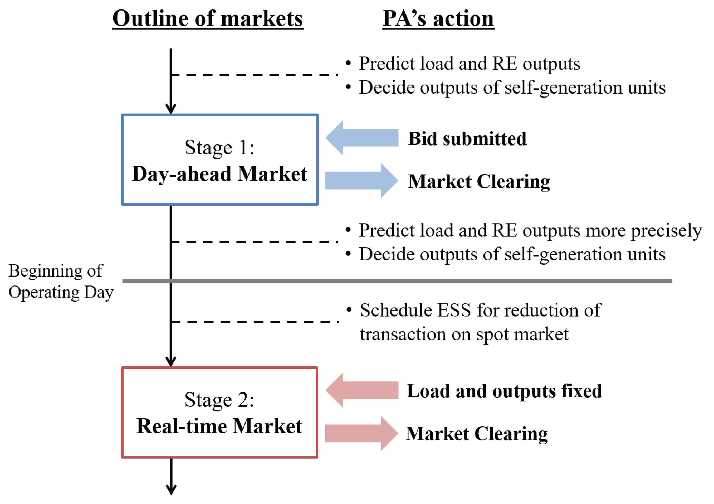Multi-period markets include forward and spot markets, used to hedge against price risks, and are used for many kinds of economic goods [1]. Even within the context of electricity markets, there are many types of multi-period markets, including a day-ahead market (DAM) and real-time market (RTM), a DAM and hourly ahead market and a DAM and imbalanced payments. Specifically, we focus on a set of DAMs and RTMs, which PAs can use to reduce the risks associated with an increase in procurement costs. Second, we consider that PAs own their ESSs, such as large-scale batteries. In order to minimize procurement costs, ESSs can be used for time arbitrage in a DAM and to reduce the number of transactions in the DAM. The former means that PAs earn profits by charging low and discharging high in their ESSs. The latter indicates that PAs avoid purchasing or selling electricity on an RTM at unfavorable prices. Although ESSs can be used to avoid unexpected increases in procurement costs, PAs have to install the appropriate size of ESS, owing to the high costs of such systems.

Many previous studies have addressed the energy procurement problem (EPP), with uncertainties, of different kinds of PAs in deregulated electricity markets [2,3,4,5,6,7,8], including studies that focus on single-period markets. In the case of electricity markets, there are two major approaches used to evaluate the impact of uncertainties: a scenario-based approach and a probabilistic approach. The advantage of a scenario-based approach is that the type of optimization problem is retained, resulting in it being employed in numerous studies [2,3,4,5,6]. However, the disadvantage of the approach is that the scale of a problem becomes much larger, based on the number of scenarios. This is why the number of scenarios is limited. As a result, several effective methods to reduce the number of scenarios have been proposed [5,6,9,10]. Of course, it is important to eliminate unnatural scenarios that are not based on actual historical data, but instead are generated by algorithms. However, it is better to deal with a larger number of scenarios in order to consider a wider variety of scenarios, especially if a large amount of actual data is available. On the other hand, a probabilistic approach assumes probability density functions and evaluates uncertainty using mean values or variances. This kind of approach is also used [7,8] because it can consider an entire case within a probability distribution. However, it is difficult to derive exact solutions in this way because formulations can be nonlinear.

In addition to previous studies related to the EPP, researchers have focused on ESSs in multi-period markets [11,12,13,14,15], considering the size and scheduling of an ESS in order to maximize profits or to minimize procurement costs. For example, studies have examined time arbitrage [14] and how to reduce payment imbalances [15]. However, to the best of our knowledge, few studies have attempted to determine the size and schedule of an ESS based on both time arbitrage and reductions in RTM transactions, although these specifications could differ depending on each purpose.

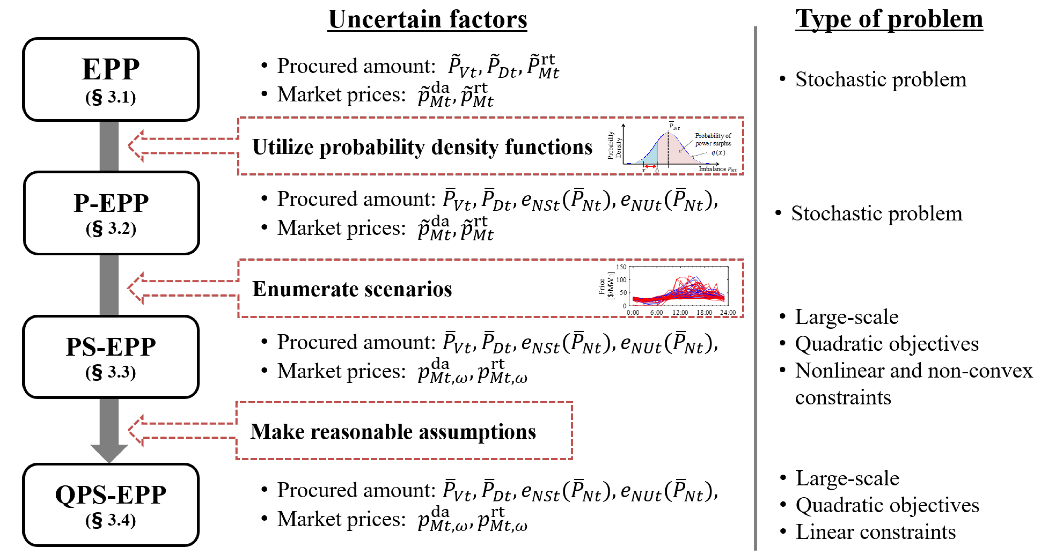
Based on the above discussion, our literature review identified the following two issues. First, there are difficulties in dealing with the large number of scenarios in scenario-based approaches and in deriving exact solutions using probabilistic approaches. Second, there is insufficient consideration of the two different purposes when determining the size and scheduling of an ESS. To address the first issue, we employ both a scenario-based and a probabilistic approach to evaluate the uncertainties, preserving the advantages of each approach. The proposed combined approach makes the optimization problem more difficult owing to its large scale and nonlinearity. However, we propose finding exact solutions within a realistic computational burden by making reasonable assumptions. To address the second issue, we employ the concepts of “slow” and “fast” ESSs, as proposed in [16,17], which enable us to divide the effects of means and variances. This study shows that slow and fast ESSs can quantify the time arbitrage in a DAM and reduce the number of transactions in an RTM, respectively. In order to verify the effectiveness of our proposed approach, we perform simulations using a generalized model of electricity markets, as well as a large amount of actual historical data.

2. Overview of Procurement Agencies and Multi-Period Markets

This section explains the models of PAs and markets used in this study.

2.1. Procurement Agency

Previous studies have modeled players who procure electricity from multiple sources, such as load-serving entities [2,7], electric retailers [4,5,8,15] and large consumers [3,6]. We model such a player as a “procurement agency (PA),” without loss of generality. As in other models, PAs supply electricity for contracted demand by procuring from multiple sources, such as bilateral contracts and self-generation. In this study, a PA has the following sources of electricity: transactions in DAMs and RTMs, self-generation, PVs and ESSs in an area. The capacity of each option is given, except in the case of ESSs. Moreover, it is assumed that a PA is a price-taker in the markets, which means its behavior has no impact on market prices.

2.2. Multi-Period Markets

Of the several types of multi-period markets, this study focuses on the following two-period energy markets: a DAM and an RTM. Figure 1 shows the market scheme and the PA’s action in each step. First, on the day before the operating day, bids are submitted to the DAM before the DAM and RTM prices and the RE outputs become known. Second, the DAM is cleared based on bidding curves by the beginning of the operating day (usually around noon on the day before). Third, RE outputs are committed just before the RTM is cleared at each hour, and PAs decide on their schedules of self-generation and the charging/discharging of their ESSs in order to supply the demand. Fourth, PA imbalances are settled after the RTM is cleared.

3. Optimization Problem of Probabilistic Procurement

This section formulates the EPP with uncertainties, as well as the procedure used to solve the problem, as shown in Figure 2. The original model of the EPP with uncertainties is formulated in Section 3.1. Then, the problem is reformulated and relaxed in Section 3.2, Section 3.3 and Section 3.4. In the process of formulating the problem, we propose an evaluation method that considers both a probabilistic distribution and scenarios, resulting in a large-scale nonlinear problem with non-convex constraints. Therefore, we make several reasonable assumptions in order to solve the formulated problem.

3.1. Energy Procurement Problem

First, the original EPP is formulated. Note that the formulation in this step does not include the reduction terms of RTM transactions. Moreover, we employ a model of multi-period markets, where both markets have the same time steps for their transactions.

Referring to previous studies of the EPP in a single market [3,5,6] and in multi-period markets [12], the objective function of the EPP in this study is given as follows.

3.1.1. Objective Function

$$\begin{array}{c}\hfill \underset{\mathit{x}}{min}{p}_E^{\mathrm{dur}}{C}_E+\sum _{t=1}^{\tau }\left(\begin{array}{c}{\displaystyle \sum _{k=1}^{n_G}(p_{G2,k}{P}_{Gk,t}^2+p_{G1,k}{P}_{Gk,t}+p_{G0,k})}\hfill \\ +{\tilde{p}}_{Mt}^{\mathrm{da}}{P}_{Mt}^{\mathrm{da}}+{\tilde{p}}_{Mt}^{\mathrm{rt}}{\tilde{P}}_{Mt}^{\mathrm{rt}}\hfill \end{array}\right),\end{array}$$

(1)

where $\mathit{x}:={[{\mathit{C}}_E,{\mathit{P}}_G,{\mathit{P}}_M^{\mathrm{da}},{\tilde{\mathit{P}}}_M^{\mathrm{rt}},{\mathit{P}}_E,\mathit{S}]}^T$.

Here, Equation (1) is the objective function used to minimize the total costs of power procurement for one settlement period, $\tau$. In this case, $\tau =24$, and the time step is set to 1 h. The first term represents the investment cost of an ESS with capacity $C_E$. This is converted to an operating cost after annualizing the investment cost from the price of the ESS using Equation (2):

$$p_E^{\mathrm{dur}}=\frac{\tau }{8760}\frac{r^{\mathrm{dis}}{p}_E}{1-{(1+r^{\mathrm{dis}})}^{-y_E}},$$

(2)

where $r^{\mathrm{dis}}$ and $y_E$ are the discount rate and the useful lifetime of the ESS (in years), respectively, and 8760 corresponds to $\tau \times 365$. The second term in Equation (1) indicates the operational cost of self-generation units, such as thermal power plants. Here, $P_{Gk,t}$ denotes the output of the k-th conventional generator, running from one to $n_G$, and $p_{Gn,k}$ is a polynomial coefficient of the n-th term in the fuel-cost function of the k-th generator. The fourth and fifth terms denote purchasing/selling electricity on a DAM and an RTM at time t ($P_{Mt}^{\mathrm{da}}$ and $P_{Mt}^{\mathrm{rt}}$, respectively), at market prices ${\tilde{p}}_{Mt}^{\mathrm{da}}$ and ${\tilde{p}}_{Mt}^{\mathrm{rt}}$, respectively. Here, $P_{Mt}^{\mathrm{da}}$ and $P_{Mt}^{\mathrm{rt}}$ refer to purchased power if positive and sold power if negative.

3.1.2. Constraints

Load Obligation with a PA in Multi-Period Markets:

$$\sum _{k=1}^{n_G}{P}_{Gk,t}+{\tilde{P}}_{Vt}+P_{Mt}^{\mathrm{da}}+P_{Et}-{\tilde{P}}_{Dt}+{\tilde{P}}_{Mt}^{\mathrm{rt}}=0,$$

(3)

where ${\tilde{P}}_{Vt}$ denotes the PV outputs at t and $P_{Et}$ denotes discharging in an ESS at t if positive and charging if negative. In addition, ${\tilde{P}}_{Dt}$ denotes the electricity demand at t. This constraint on the PA’s load obligation shows that it has to purchase/sell electricity on an RTM if there is a mismatch between power demand and supply at t owing to uncertainties ${\tilde{P}}_{Vt}$ and ${\tilde{P}}_{Dt}$.

Limitation of the Output of Conventional Power Plants:

$$P_{Gk}^{min}\le P_{Gk,t}\le P_{Gk}^{max},$$

(4)

$$\left|P_{Gk,t+1}-P_{Gk,t}\right|\le \Delta P_{Gk}.$$

(5)

Here, Equations (4) and (5) represent the upper and lower limits of the generator output ($P_{Gk}^{max}$ and $P_{Gk}^{min}$, respectively) and the upper and lower limits of the rate of change of generation ($\Delta P_{Gk}$).

Relational Expression for Charging/Discharging and State of Charge:

$$S_{t+1}-S_t=-P_{Et},$$

(6)

where $S_t$ is the charge state of a slow ESS at t.

Limitation of State of Charge:

$$0\le S_t\le C_E,$$

(7)

where $C_E$ is the capacity of an ESS.

In summary, the EPP has stochastic parameters and variables, and thus, transformations are required in order to solve the problem.

3.2. Probabilistic EPP

Based on the formulation of the EPP, probabilistic indices are employed to evaluate the uncertainties. The modeling targets in this section are ${\tilde{P}}_{Vt}$ and ${\tilde{P}}_{Dt}$ in order to quantify the expectations of purchasing/selling electricity on an RTM. In order to simplify the modeling of the indices, we assume that the PV output and the demand for 1 h follow a Gaussian distribution. The use of other probability distributions is reserved for future work.

Equation (8) denotes the expected imbalances after DAM clearing, based on ${\overline{P}}_{Vt}$ and ${\overline{P}}_{Dt}$, and the expectations of ${\tilde{P}}_{Vt}$ and ${\tilde{P}}_{Dt}$:

$${\overline{P}}_{Nt}=\sum _{k=1}^{n_G}{P}_{Gk,t}+{\overline{P}}_{Vt}+P_{Mt}^{\mathrm{da}}+P_{Et}-{\overline{P}}_{Dt}.$$

(8)

The negative and positive values of ${\overline{P}}_{Nt}$ denote a power shortage and surplus, respectively. PAs have to purchase electricity from the RTM in the case of a shortage and have to sell electricity in the RTM in the case of a surplus.

In addition, Equation (9) shows that ${\overline{P}}_{Nt}$ is bounded by the upper and lower limits of ${\overline{P}}_{Nt}$, $P_{Nt}^{max}$ and $P_{Nt}^{min}$, respectively:

$$P_{Nt}^{min}\le {\overline{P}}_{Nt}\le P_{Nt}^{max}.$$

(9)

From the viewpoint of transactions in multi-period markets, both $P_{Nt}^{max}$ and $P_{Nt}^{min}$ denote the degree of virtual bidding allowed on a DAM. If $P_{Nt}^{max}$ and $P_{Nt}^{min}$ are set to zero, the secondary market can be regarded as a system of imbalanced payments because it is prohibited from practicing arbitrage between the two markets.

Equation (10) shows the relational expression for the standard deviation of imbalances, ${\sigma }_{Nt}$:

$${\sigma }_{Nt}^2={\sigma }_{Vt}^2+{\sigma }_{Dt}^2+2{\sigma }_{VDt},$$

(10)

where ${\sigma }_{Vt}$, ${\sigma }_{Dt}$ and ${\sigma }_{VDt}$ indicate the standard deviations of ${\tilde{P}}_{Vt}$ and ${\tilde{P}}_{Dt}$ and the covariance between ${\tilde{P}}_{Vt}$ and ${\tilde{P}}_{Dt}$, respectively. Here, the standard deviations of the imbalances are simply parameters, because they do not include any decision variables.

Using this assumption for the probability density function, $q(x;{\overline{P}}_{Nt},{\sigma }_{Nt})$, two probabilistic indices are formulated: expected energy not supplied (EENS, $e_{\mathit{NS}t}$) [18] and expected energy not used (EENU, $e_{\mathit{NU}t}$) [19], as shown in Equations (11) and (12). The former measures the incidence of power shortages, denoting expected purchases of electricity, and the latter is a metric for power surpluses, denoting the expected selling of electricity in the RTM:

$$\begin{array}{c}\hfill \begin{array}{ccc}\hfill e_{\mathit{NS}t}({\overline{P}}_{Nt};{\sigma }_{Nt})& =& {\int }_{-\infty }^0(-x)q(x;{\overline{P}}_{Nt},{\sigma }_{Nt})dx\hfill \\ & =& \frac{{\sigma }_{Nt}}{\sqrt{2}}\left(z_t(\mathrm{erf}\left(z_t\right)-1)+\frac{exp(-z_t^2)}{\sqrt{\pi }}\right),\hfill \end{array}\end{array}$$

(11)

$$\begin{array}{c}\hfill \begin{array}{ccc}\hfill e_{\mathit{NU}t}({\overline{P}}_{Nt};{\sigma }_{Nt})& =& {\int }_0^{\infty }xq(x;{\overline{P}}_{Nt},{\sigma }_{Nt})dx\hfill \\ & =& \frac{{\sigma }_{Nt}}{\sqrt{2}}\left(z_t(\mathrm{erf}\left(z_t\right)+1)+\frac{exp(-z_t^2)}{\sqrt{\pi }}\right),\hfill \end{array}\end{array}$$

(12)

where $z_t$ can be expressed as Equation (13), and $\mathrm{erf}(·)$ denotes the error function, as shown in Equation (14):

$$z_t=\frac{{\overline{P}}_{Nt}}{\sqrt{2}{\sigma }_{Nt}},$$

(13)

$$\mathrm{erf}\left(x\right)=\frac{2}{\sqrt{\pi }}{\int }_0^{x}exp(-X^2)dX.$$

(14)

Therefore, the expected purchasing/selling of electricity in the RTM is given as Equation (15):

$$E[{\tilde{P}}_{Mt}^{\mathrm{rt}}]=\left\{\begin{array}{cc}{e_{NS}}_t\left({\overline{P}}_{Nt}\right)\hfill & \mathrm{if}{P}_{Mt}^{\mathrm{rt}}\ge 0,\hfill \\ -{e_{NU}}_t\left({\overline{P}}_{Nt}\right)\hfill & \mathrm{otherwise}.\hfill \end{array}\right.$$

(15)

Thus, the part of the objective function related to transaction costs in the RTM (set to $f_M^{\mathrm{rt}}$) can be formulated as Equation (16):

$$f_M^{\mathrm{rt}}\left({\overline{P}}_{Nt}\right)=\sum _{t=1}^{\tau }{\tilde{p}}_{Mt}^{\mathrm{rt}}\left\{{e_{NS}}_t\left({\overline{P}}_{Nt}\right)-{e_{NU}}_t\left({\overline{P}}_{Nt}\right)\right\}.$$

(16)

In the next step, we model the reduction in RTM transactions by charging and discharging within an ESS, because the price of the DAM is usually unfavorable to a PA.

$$f_M^{\mathrm{rt}}({\overline{P}}_{Nt},e_{NSt}^{\mathrm{red}},e_{NUt}^{\mathrm{red}})=\sum _{t=1}^{\tau }\left(\begin{array}{c}{\tilde{p}}_{Mt}^{\mathrm{rt}}\left\{({e_{NS}}_t\left({\overline{P}}_{Nt}\right)-e_{NSt}^{\mathrm{red}})-({e_{NU}}_t\left({\overline{P}}_{Nt}\right)-e_{NUt}^{\mathrm{red}})\right\}\hfill \\ +p_E^{\mathrm{dur}}(e_{NSt}^{\mathrm{red}}+e_{NUt}^{\mathrm{red}})\hfill \end{array}\right),$$

(17)

where $e_{NSt}^{\mathrm{red}}$ and $e_{NUt}^{\mathrm{red}}$ indicate the expected reductions in purchases and sales of electricity at t, respectively. Here, the term $p_E^{\mathrm{dur}}(e_{NSt}^{\mathrm{red}}+e_{NUt}^{\mathrm{red}})$ is added as the investment cost of an ESS associated with reducing the number of RTM transactions.

In the following step, $e_{NSt}^{\mathrm{red}}$ and $e_{NUt}^{\mathrm{red}}$ are determined, but it is required that PAs derive the size of an ESS to be installed. Therefore, a term with the same dimension as ${\overline{P}}_{Nt}$ can be extracted from the difference between the original expected electricity transaction and the reduced transaction using the inverse functions of EENS and EENU, as shown in Equations (18) and (19).

$$\begin{array}{c}\hfill \begin{array}{ccc}\hfill P_{Et}^{\mathrm{fs}}& =& e_{NSt}^{-1}\left(e_{NSt}\left({\overline{P}}_{Nt}\right)\right)-e_{NSt}^{-1}(e_{NSt}\left({\overline{P}}_{Nt}\right)-e_{NSt}^{\mathrm{red}})\hfill \\ & =& {\overline{P}}_{Nt}-e_{NSt}^{-1}(e_{NSt}\left({\overline{P}}_{Nt}\right)-e_{NSt}^{\mathrm{red}}),\hfill \end{array}\end{array}$$

(18)

$$\begin{array}{c}\hfill \begin{array}{ccc}\hfill P_{Et}^{\mathrm{fu}}& =& e_{NUt}^{-1}\left(e_{NUt}\left({\overline{P}}_{Nt}\right)\right)-e_{NUt}^{-1}(e_{NUt}\left({\overline{P}}_{Nt}\right)-e_{NUt}^{\mathrm{red}})\hfill \\ & =& {\overline{P}}_{Nt}-e_{NUt}^{-1}(e_{NUt}\left({\overline{P}}_{Nt}\right)-e_{NUt}^{\mathrm{red}}).\hfill \end{array}\end{array}$$

(19)

The new variables, $P_{Et}^{\mathrm{fs}}$ and $P_{Et}^{\mathrm{fu}}$, constrain purchases and sales of electricity caused by sudden changes in power supply and demand. Thus, these variables can be regarded as “fast” discharging and charging in an ESS. Here, we refer to these as “fast” ESSs for shortages ($P_{Et}^{\mathrm{fs}}$) and surpluses ($P_{Et}^{\mathrm{fu}}$). In order to simplify the problem, we assume that fast ESSs for shortages and surpluses can only discharge and charge, respectively. Based on this assumption, the required capacities of fast ESSs, $C_E^{\mathrm{fs}}$ and $C_E^{\mathrm{fu}}$, can be easily determined, as expressed in Equations (20) and (21).

$$C_E^{\mathrm{fs}}=\sum _{t=1}^{\tau }{P}_{Et}^{\mathrm{fs}}$$

(20)

$$C_E^{\mathrm{fu}}=\sum _{t=1}^{\tau }(-P_{Et}^{\mathrm{fu}}).$$

(21)

In order to distinguish a conventional ESS ($P_{Et},C_E$) from a fast ESS, we refer to ESSs that do not consider uncertainties as “slow” ESSs.

Using the characteristics related to ${e_{NS}}_t\left({\overline{P}}_{Nt}\right)$ and ${e_{NU}}_t\left({\overline{P}}_{Nt}\right)$, as shown in Equation (22), Equation (17) can be simplified as shown in Equation (23):

$$\begin{array}{c}\hfill \begin{array}{ccc}\hfill E[{\tilde{P}}_{Mt}^{\mathrm{rt}}]& =& {e_{NS}}_t\left({\overline{P}}_{Nt}\right)-{e_{NU}}_t\left({\overline{P}}_{Nt}\right)\hfill \\ & =& {\int }_{-\infty }^0(-x)q\left(x\right)dx-{\int }_0^{\infty }xq\left(x\right)dx\hfill \\ & =& -{\int }_{-\infty }^{\infty }xq\left(x\right)dx\hfill \\ & =& -{\overline{P}}_{Nt},\hfill \end{array}\end{array}$$

(22)

$$\begin{array}{c}\hfill \begin{array}{ccc}\hfill f_M^{\mathrm{rt}}({\overline{P}}_{Nt},e_{NSt}^{\mathrm{red}},e_{NUt}^{\mathrm{red}})& =& {\sum }_{t=1}^{\tau }\left(\begin{array}{c}-{\tilde{p}}_{Mt}^{\mathrm{rt}}{\overline{P}}_{Nt}\hfill \\ +(p_E^{\mathrm{dur}}-{\tilde{p}}_{Mt}^{\mathrm{rt}})e_{NSt}^{\mathrm{red}}+(p_E^{\mathrm{dur}}+{\tilde{p}}_{Mt}^{\mathrm{rt}})e_{NUt}^{\mathrm{red}}\hfill \end{array}\right).\hfill \end{array}\end{array}$$

(23)

Finally, Equations (24) and (25) must be installed to keep the amount of electricity purchased/sold non-negative:

$$0\le e_{NSt}^{\mathrm{red}}\le e_{NSt}\left({\overline{P}}_{Nt}\right),$$

(24)

$$0\le e_{NUt}^{\mathrm{red}}\le e_{NUt}\left({\overline{P}}_{Nt}\right).$$

(25)

These are reverse-convex constraints because both $e_{NSt}({\overline{P}}_{Nt})$ and $e_{NUt}({\overline{P}}_{Nt})$ are convex functions (see Appendix A).

In summary, the probabilistic EPP (P-EPP) is formulated as follows:

$$\begin{array}{cc}\hfill \underset{\mathit{x}}{min}& p_E^{\mathrm{dur}}{C}_E+\sum _{t=1}^{\tau }\left(\begin{array}{c}{\displaystyle \sum _{k=1}^{n_G}(p_{G2,k}{P}_{Gk,t}^2+p_{G1,k}{P}_{Gk,t}+p_{G0,k})}\hfill \\ +{\tilde{p}}_{Mt}^{\mathrm{da}}{P}_{Mt}^{\mathrm{da}}-{\tilde{p}}_{Mt}^{\mathrm{rt}}{\overline{P}}_{Nt}\hfill \\ +(p_E^{\mathrm{dur}}-{\tilde{p}}_{Mt}^{\mathrm{rt}})e_{NSt}^{\mathrm{red}}+(p_E^{\mathrm{dur}}+{\tilde{p}}_{Mt}^{\mathrm{rt}})e_{NUt}^{\mathrm{red}}\hfill \end{array}\right)\hfill \\ \hfill \mathrm{s}.\mathrm{t}.& \mathrm{Equations}\left(4\right)–\left(9\right),\left(24\right)\mathrm{and}\left(25\right).\hfill \end{array}$$

3.3. Probabilistic and Scenario-Based EPP

Even though stochastic decision variables are removed, the P-EPP includes stochastic parameters of ${\tilde{p}}_{Mt}^{\mathrm{da}}$ and ${\tilde{p}}_{Mt}^{\mathrm{rt}}$. We fix these stochastic parameters based on the number of scenarios.

Equation (26) defines the occurrence probability of the $\omega$-th scenario, with values ranging from one to $n_{\mathsf{\Omega }}$.

$$q_{M\omega }=Pr[{\tilde{p}}_{Mt}^{\mathrm{da}}=p_{Mt\omega }^{\mathrm{da}},{\tilde{p}}_{Mt}^{rt}=p_{Mt\omega }^{\mathrm{rt}}].$$

(26)

In other words, one scenario provides two prices (i.e., for the DAM and the RTM).

The variables are decided according to each scenario, so the expected procurement costs should be taken into account in the objective function. In addition, for the constraints, Equations (4)–(9), (24) and (25) are generated for each scenario. However, this does not affect the characteristics of the optimization problem. Therefore, the probabilistic and scenario-based EPP (PS-EPP) is formulated as follows:

$$\begin{array}{cc}\hfill \underset{\mathit{x}}{min}& \sum _{\omega =1}^{n_{\mathsf{\Omega }}}{q}_{M\omega }\left(p_E^{\mathrm{dur}}{C}_{E\omega }+\sum _{t=1}^{\tau }\left(\begin{array}{c}{\displaystyle \sum _{k=1}^{n_G}(p_{G2,k}{P}_{Gk,t,\omega }^2+p_{G1,k}{P}_{Gk,t,\omega }+p_{G0,k})}\hfill \\ +p_{Mt,\omega }^{\mathrm{da}}{P}_{Mt,\omega }^{\mathrm{da}}-p_{Mt,\omega }^{\mathrm{rt}}{\overline{P}}_{Nt,\omega }\hfill \\ +(p_E^{\mathrm{dur}}-p_{Mt,\omega }^{\mathrm{rt}})e_{NSt,\omega }^{\mathrm{red}}+(p_E^{\mathrm{dur}}+p_{Mt,\omega }^{\mathrm{rt}})e_{NUt,\omega }^{\mathrm{red}}\hfill \end{array}\right)\right)\hfill \\ \hfill \mathrm{s}.\mathrm{t}.& \mathrm{Equations}\left(4\right)–\left(9\right),\left(24\right)\mathrm{and}\left(25\right),\forall \omega \in \{1,\dots ,n_{\mathsf{\Omega }}\}.\hfill \end{array}$$

3.4. Quadratic Probabilistic and Scenario-Based EPP

The PS-EPP is formulated as in Section 3.3 and has a quadratic objective function. However, the feasible region consists of nonlinear and non-convex functions, as shown in Equations (24) and (25). This section describes the method to solve the PS-EPP, considering the structural features and making several reasonable assumptions.

Focusing only on the decision variables $e_{NSt,\omega }^{\mathrm{red}}$ and $e_{NSt,\omega }^{\mathrm{red}}$, the objective function of the PS-EPP is separable and linear, and both are bounded by Equations (24) and (25). Owing to these structural features, the solution of $e_{NSt,\omega }^{\mathrm{red}}$ and $e_{NSt,\omega }^{\mathrm{red}}$ can be derived automatically, as shown in Equations (27) and (28).

$$e_{NSt,\omega }^{\mathrm{red}}=\left\{\begin{array}{cc}0\hfill & \mathrm{if}{p}_E^{\mathrm{dur}}-p_{Mt,\omega }^{\mathrm{rt}}\ge 0,\hfill \\ {e_{NS}}_{t,\omega }\left({\overline{P}}_{Nt,\omega }\right)\hfill & \mathrm{otherwise},\hfill \end{array}\right.$$

(27)

$$e_{NUt,\omega }^{\mathrm{red}}=\left\{\begin{array}{cc}0\hfill & \mathrm{if}{p}_E^{\mathrm{dur}}+p_{Mt,\omega }^{\mathrm{rt}}\ge 0,\hfill \\ {e_{NU}}_{t,\omega }\left({\overline{P}}_{Nt,\omega }\right)\hfill & \mathrm{otherwise}.\hfill \end{array}\right.$$

(28)

As a result, $e_{NSt,\omega }^{\mathrm{red}}$ and $e_{NSt,\omega }^{\mathrm{red}}$ can be eliminated, and the reverse-convex constraints of Equations (24) and (25) can be ignored. Equation (29) shows the transaction costs in the RTM, after reformulating using Equations (22), (24) and (25).

$$f_M^{\mathrm{rt}}\left({\overline{P}}_{Nt,\omega }\right)=\sum _{\omega =1}^{n_{\mathsf{\Omega }}}{q}_{M\omega }\left(\begin{array}{c}{\displaystyle \sum _{t\in {\mathcal{T}}_1}\left(-p_{Mt,\omega }^{\mathrm{rt}}{\overline{P}}_{Nt,\omega }\right)}\hfill \\ {\displaystyle +\sum _{t\in {\mathcal{T}}_2}\left\{p_E^{\mathrm{dur}}{e}_{NSt,\omega }\left({\overline{P}}_{Nt,\omega }\right)-p_{Mt,\omega }^{\mathrm{rt}}{e}_{NUt,\omega }\left({\overline{P}}_{Nt,\omega }\right)\right\}}\hfill \\ {\displaystyle +\sum _{t\in {\mathcal{T}}_3}\left\{p_{Mt,\omega }^{\mathrm{rt}}{e}_{NSt,\omega }\left({\overline{P}}_{Nt,\omega }\right)+p_E^{\mathrm{dur}}{e}_{NUt,\omega }\left({\overline{P}}_{Nt,\omega }\right)\right\}}\hfill \end{array}\right),$$

(29)

where ${\mathcal{T}}_1,{\mathcal{T}}_2$ and ${\mathcal{T}}_3$ are defined as follows:

$$\begin{array}{c}\hfill \begin{array}{c}{\mathcal{T}}_1:=\{t=1,\dots ,\tau |-p_E^{\mathrm{dur}}\le p_{Mt,\omega }^{\mathrm{rt}}\le p_E^{\mathrm{dur}}\},\hfill \\ {\mathcal{T}}_2:=\{t=1,\dots ,\tau |p_E^{\mathrm{dur}}-p_{Mt,\omega }^{\mathrm{rt}}<0\},\hfill \\ {\mathcal{T}}_3:=\{t=1,\dots ,\tau |p_E^{\mathrm{dur}}+p_{Mt,\omega }^{\mathrm{rt}}<0\}.\hfill \end{array}\end{array}$$

Here, ${\mathcal{T}}_1\cap {\mathcal{T}}_2\cap {\mathcal{T}}_3=Ø$, and ${\mathcal{T}}_1\cup {\mathcal{T}}_2\cup {\mathcal{T}}_3=\{1,\dots ,\tau \}$ because $p_E^{\mathrm{dur}}$ is greater than zero.

Although non-convex constraints are eliminated, $f_M^{\mathrm{rt}}\left({\overline{P}}_{Nt,\omega }\right)$ is non-convex (and more specifically, concave; see Appendix B), which could make it difficult to find the global optimal solution. In addition, the nonlinearity could be a factor causing high computational costs.

Therefore, in order to simplify and relax the problem, we assume that ${\overline{P}}_{Nt,\omega }$ is set to $P_{Nt}^{max}$ at $t\in {\mathcal{T}}_2$ and that ${\overline{P}}_{Nt,\omega }$ is set to $P_{Nt}^{min}$ at $t\in {\mathcal{T}}_3$, showing some of the features that make these assumptions reasonable.

The first feature of the PS-EPP is that we can determine the ${\overline{P}}_{Nt,\omega }$ that minimizes $f_M^{\mathrm{rt}}\left({\overline{P}}_{Nt,\omega }\right)$ in the case of $t\in {\mathcal{T}}_2\cup {\mathcal{T}}_3$, as shown in Equations (30) and (31), because the functions are monotonically decreasing or monotonically increasing (see Appendix B):

$$\begin{array}{c}\hfill \underset{\begin{array}{c}{P}_{Nt}^{min}\le {\overline{P}}_{Nt,\omega }\le P_{Nt}^{max},\\ \forall t\in {\mathcal{T}}_2\end{array}}{argmin}\{p_E^{\mathrm{dur}}{e}_{NSt,\omega }\left({\overline{P}}_{Nt,\omega }\right)-p_{Mt,\omega }^{\mathrm{rt}}{e}_{NUt,\omega }\left({\overline{P}}_{Nt,\omega }\right)\}=P_{Nt}^{max}\end{array}$$

(30)

$$\begin{array}{c}\hfill \underset{\begin{array}{c}{P}_{Nt}^{min}\le {\overline{P}}_{Nt,\omega }\le P_{Nt}^{max},\\ \forall t\in {\mathcal{T}}_3\end{array}}{argmin}\{p_{Mt,\omega }^{\mathrm{rt}}{e}_{NSt,\omega }\left({\overline{P}}_{Nt,\omega }\right)+p_E^{\mathrm{dur}}{e}_{NUt,\omega }\left({\overline{P}}_{Nt,\omega }\right)\}=P_{Nt}^{min}.\end{array}$$

(31)

Note that the global optimal solution is not guaranteed, because ${\overline{P}}_{Nt,\omega }$ is fixed considering only $f_M^{\mathrm{rt}}\left({\overline{P}}_{Nt,\omega }\right)$, even though Equation (8) includes ${\overline{P}}_{Nt,\omega }$.

The second feature is that the fixed ${\overline{P}}_{Nt,\omega }$ at $t\in {\mathcal{T}}_2\cup {\mathcal{T}}_3$ does not conflict with reasonable PA actions in the RTM. Specifically, in the case of $t\in {\mathcal{T}}_2\cup {\mathcal{T}}_3$, the real-time (RT) price is so unfavorable as to install an ESS, as described in the inequality constraints. This is why $e_{NSt,\omega }^{\mathrm{red}}$ and $e_{NSt,\omega }^{\mathrm{red}}$ should be greater than zero, which means installing fast ESSs.

Finally, the quadratic PS-EPP (QPS-EPP) can be formulated as follows:

$$\begin{array}{cc}\hfill \underset{\mathit{x}}{min}& \sum _{\omega =1}^{n_{\mathsf{\Omega }}}{q}_{M\omega }\left(\begin{array}{c}{p}_E^{\mathrm{dur}}{C}_{E\omega }\hfill \\ {\displaystyle +\sum _{t=1}^{\tau }\left({\displaystyle \sum _{k=1}^{n_G}(p_{G2,k}{P}_{Gk,t,\omega }^2+p_{G1,k}{P}_{Gk,t,\omega }+p_{G0,k})+p_{Mt,\omega }^{\mathrm{da}}{P}_{Mt,\omega }^{\mathrm{da}}}\right)}\hfill \\ {\displaystyle +\sum _{t\in {\mathcal{T}}_1}(-p_{Mt,\omega }^{\mathrm{rt}}{\overline{P}}_{Nt,\omega })}\hfill \end{array}\right)\hfill \\ \hfill \mathrm{s}.\mathrm{t}.& \mathrm{Equations}\left(4\right)–\left(9\right)\hfill \\ & {\overline{P}}_{Nt,\omega }=P_{Nt}^{max},\forall t\in {\mathcal{T}}_2\hfill \\ & {\overline{P}}_{Nt,\omega }=P_{Nt}^{min},\forall t\in {\mathcal{T}}_3\hfill \\ & \forall \omega \in \{1,\dots ,n_{\mathsf{\Omega }}\}.\hfill \end{array}$$

This optimization problem can be solved easily using quadratic programming, even if the scale of the problem is large.

4. Simulation

4.1. Parameter Setting and Data

This section describes the parameters related to a PA and to the multi-period markets. As described in Section 2.1, a PA has the following procurement sources: transactions in a DAM and an RTM, self-generation, PVs and ESSs.

4.1.1. PVs and Contracted Demands

The capacity of PVs and the contracted demand are set to 50 MW and 100 MW, respectively. Moreover, we use data provided by Pennsylvania-New Jersey-Maryland interconnection (PJM)through Data Miner 2 [20] to create the profiles for PV output and demand for the operating day. Specifically, PV output uses data on generating power based on the fuel type of “solar” [21]. Then, the demand is hourly data of metered loads in PJM (RTO region) [22]. Both sets of data cover the period 1 July 2017–30 September 2017, because they both include seasonal characteristics. Then, both sets of data are adjusted using the capacity of PVs and the contracted demand, comparing them with the maximum values for the study period. 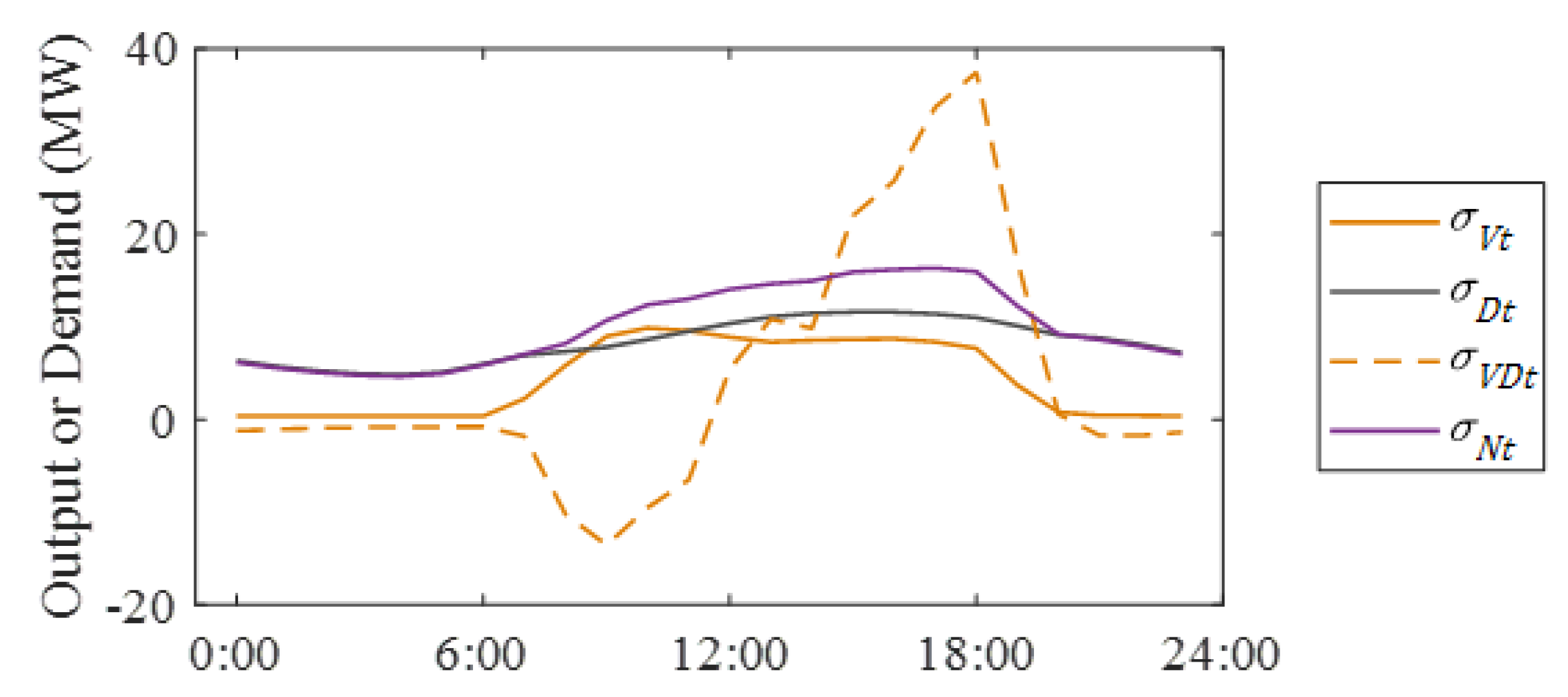Figure 3 shows the mean PV output (${\overline{P}}_{Vt}$) and mean demand (${\overline{P}}_{Dt}$) for the study period, as well as the standard deviations of imbalances (${\sigma }_{Nt}$), derived from each standard deviation and the covariance (i.e., ${\sigma }_{Vt}$, ${\sigma }_{Dt}$ and ${\sigma }_{VDt}$).

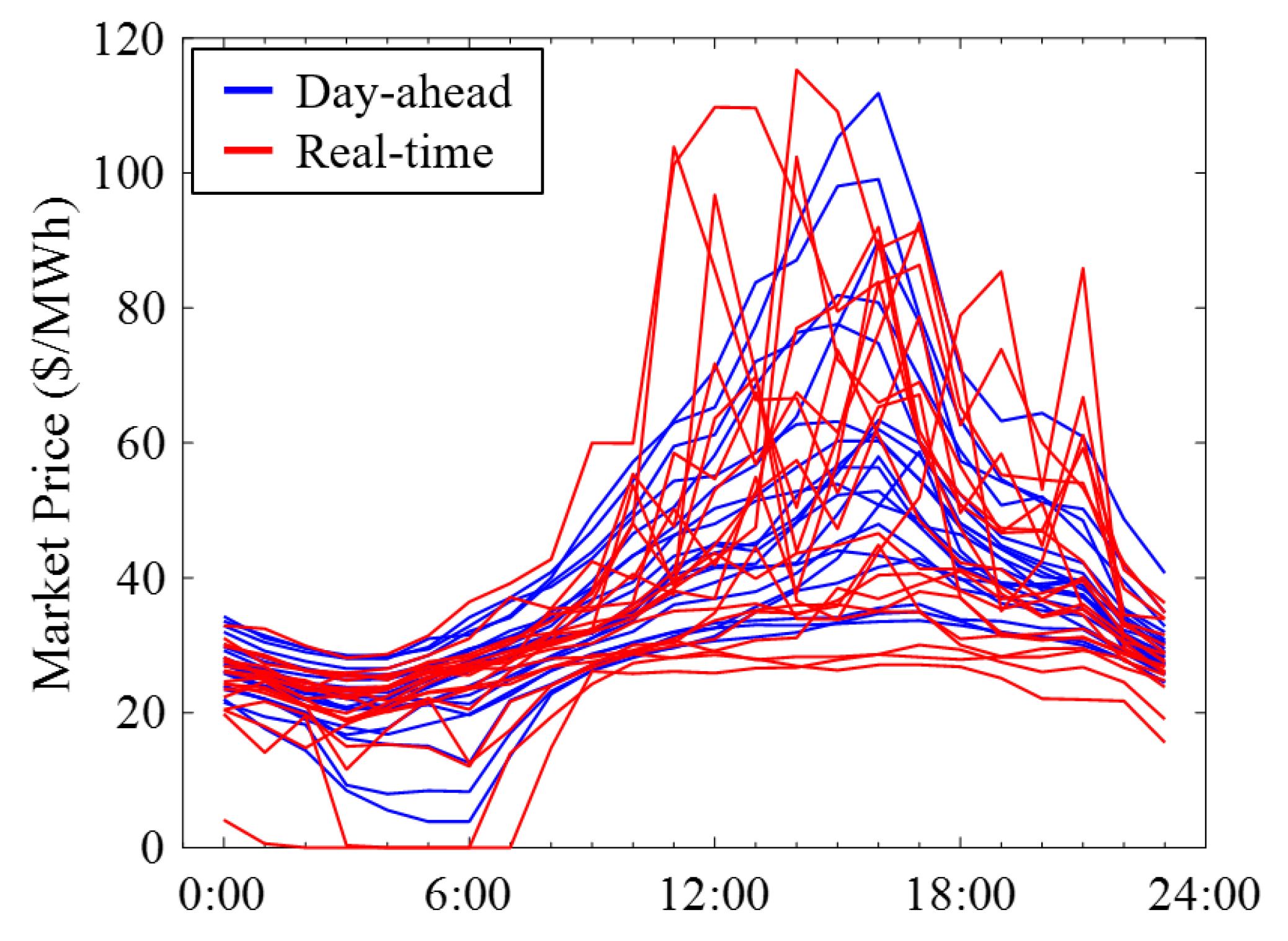
4.1.2. Market Prices

We use the data on prices in the DAM and RTM given in PJM (pricing node: PJM-RTO) [23,24], as well as the PV output and demand. The data cover the period 1 July–30 September, which is the same period used for the PV output and demand, for the four years between 2014 and 2017. Therefore, there are 368 scenarios. The probability of each scenario is divided equally: $q_{M\omega }=1/368$. Figure 4 shows samples of the DAM and RTM prices.

4.1.3. Self-Generation

The number of self-generating units is set to one (i.e., $n_G=1$), and the type of generator is set as an oil-fired power plant as a dispatchable generator. The capacity of generation is set to 100 MW, and all parameters are taken from the generation unit at bus 7 in the IEEE Reliability Test System (RTS) [25]. As for the generation costs for the above unit, $p_{G2}$, $p_{G1}$ and $p_{G0}$ are $0.05\$/{\mathrm{MW}}^2$, $43.66\$/\mathrm{MW}$ and $781.52\$/\mathrm{h}$, respectively. The parameters related to generator outputs are as follows: $P_G^{min}$, $P_G^{max}$ and $\Delta P_G$ are set to 0 MW, 100 MW and 100 MW, respectively.

4.1.4. ESSs

The installation cost of an ESS, $p_E$, is 0.50 million [26], and the daily cost of an ESS, $p_E^{\mathrm{dur}}$, is 177 $/day, from Equation (2). Moreover, we add upper limits to the installed capacities of ESSs of 50 MWh, which is equal to the size of settled PVs. This is because the optimization problem is unbounded in some cases.

4.1.5. Others

All the simulations in Section 3 are carried out on a computer configured as Intel(R) Core(TM) i7-6700 CPU (Intel Corporation, Santa Clara, CA, USA) 3.40 GHz and 32.0 GB of RAM and using MATLAB (2017a, The MathWorks, Inc., Natick, MA, USA).

4.2. Simulation Results

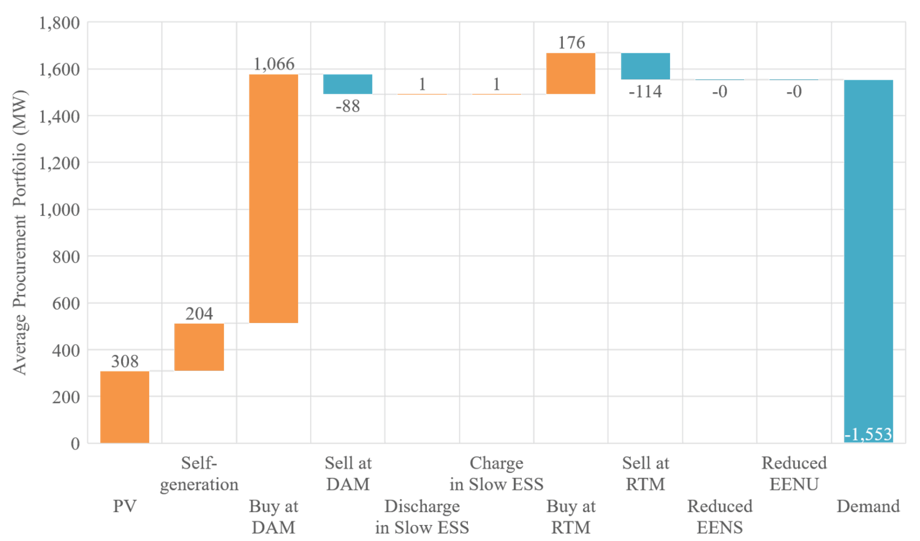
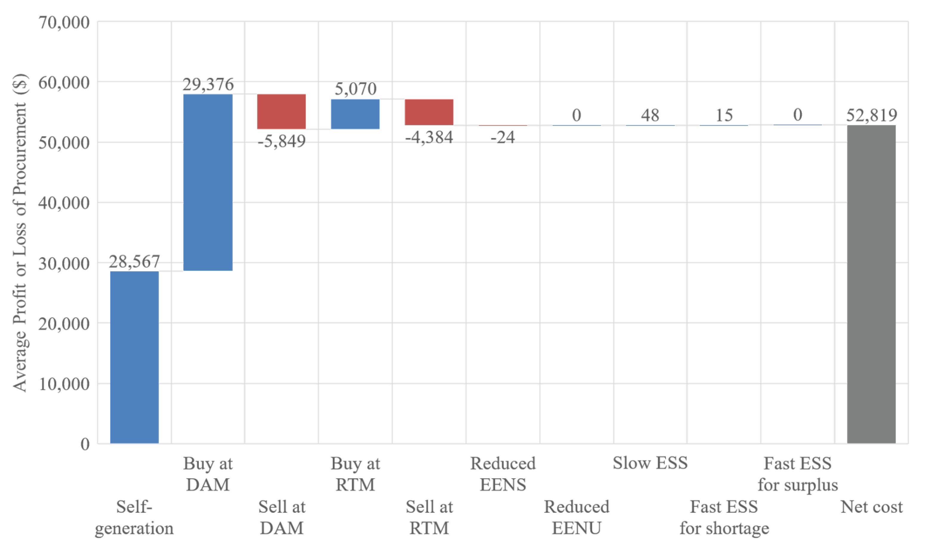
Figure 5 and Figure 6 shows the aggregated results of all scenarios derived from the QPS-EPP. Figure 5 shows the average profit and loss of procurement, divided into each source, and Figure 6 shows the average power procurement portfolio for all scenarios. Several findings are evident from these simulation results: (1) the amount of procured electricity from self-generation is not large, but the procurement cost is high; (2) PAs procure electricity mainly from a DAM; (3) the amount of electricity sold is smaller than bought; and (4) ESSs are only installed in a few cases.

First, almost half the total procurement cost is for self-generation, with the remainder comprising purchases from the DAM. On the other hand, the amount of power procured from the DAM is much larger than that from self-generation. This is because of the generation cost is independent of $P_{Gt}$ (i.e., ${\sum }_{t=1}^{\tau }{p}_{G0}=\mathrm{18,756}$). However, some results described later show that self-generation is used effectively when the price on the DAM is relatively high.

Second, PAs bought a large amount of electricity on the DAM because this market had the greatest price advantage. This is obvious after comparing the amount of bought electricity and the procured amount.

Third, the amount of electricity sold is smaller than that bought. The first reason for this is that the operating duration was mainly in summer, when power shortages often occur, which may have resulted in higher market prices. The second reason is that the size of settled PVs is not sufficient to cause power surpluses. Even though power shortages are likely to occur in the overall market, PAs that have large sources can sell electricity in the markets. PV output is the best source of electricity to be sold because the operational costs are zero. However, PAs do not have sufficient PVs for this option.

Fourth, as shown in Figure 5 and Figure 6, the sizes of the slow and fast ESSs are small, overall. This is obviously because of their high costs, although both ESSs were installed and used effectively and sufficiently in some cases.

Figure 7 and Figure 8 shows some of the cases when ESSs were installed and utilized, including the operations in each scenario. The first figure shows the procurement result on 25 September 2017, when slow ESSs were installed and utilized. The second figure shows the result on 20 July 2015, when fast ESSs were installed. In general, as shown in Figure 7 and Figure 8, PAs procure electricity from the DAM when the day-ahead (DA)price is low and use self-generation when the price is high. Moreover, ${\overline{P}}_{Nt,\omega }$ is $P_{Nt}^{max}$ in the case of $p_{Mt,\omega }^{\mathrm{rt}}>p_{Mt,\omega }^{\mathrm{da}}$, and vice versa.

On 25 September 2017, slow ESSs were installed up to the upper limits because the DA price was relatively higher than on other days. Given the expected operation at $t=1$, slow ESSs were charged when the DA price was lower and then discharged immediately after the price increased. This means that arbitrage using slow ESSs in the DAM was practiced perfectly. On the other hand, fast ESSs were not installed because the real-time (RT)price was low. Moreover, the amount of electricity bought on the RTM was large because the RT price was lower than the DA almost all day, resulting in ${\overline{P}}_{Nt,\omega }=P_{Nt}^{min}$.

On 20 July 2015, fast ESSs for shortages were installed and discharged at some t in the case of $p_{Mt,\omega }^{\mathrm{rt}}>p_E^{\mathrm{dur}}=177$. As a result, PAs were able to avoid buying electricity on the RTM. The sizes of the installed fast ESSs, $C_E^{\mathrm{fs}}$, were 139.7 MWh, which depended on ${\overline{P}}_{Vt}$ and ${\overline{P}}_{Dt}$, owing to the functions ${e_{NS}}_{t,\omega }$.

Finally, we explain the principal used to determine the size of an installed slow and fast ESSs, based on simulation results and the above discussion.

Table 1. Data of ESS installation.

Type of ESS	Minimum Capacity (MWh)	Maximum Capacity (MWh)	Average Capacity (MWh)	Number of Cases Procured from ESSs	Average for Days with ESSs (MWh)
Slow ESS	0	50.0	0.3	2	50.0
Fast ESS for shortage	0	203.6	2.3	10	86.2
Fast ESS for surplus	0	0	0	0	0

shows the data on ESS sizes, which include the minimum, maximum and average capacity of each ESS in all scenarios, the number of scenarios in which each ESS was installed and the average capacity of each ESS among those scenarios. Several viewpoints can be considered by decision-makers when determining the size of each ESS: conservative, cost-savings and balanced. First, conservative decision-makers should install the maximum size because they can avoid paying more than usual in any cases considered. Second, cost-saving-minded decision-makers should install the minimum or average sizes for all scenarios. However, it might be meaningless to install a limited size of ESS, because a certain size is required to adapt to a day when PAs charge or discharge ESSs. Third, balanced-minded decision-makers should install the average size for days with ESSs, because this will enable them to employ intermediate scenarios, when PAs without ESSs could pay more. Regardless of the nature of a decision-maker, we need to note the following. The simulation results are based only on the given scenarios, and are underestimated owing to certain assumptions. In addition, decision-makers should consider how to utilize ESSs in ways other than arbitrage and to reduce payments in an RTM, such as ancillary services and demand response programs.

5. Conclusions

Minimizing the procurement costs of electricity is a critical problem for PAs, but multiple factors associated with uncertainties are inevitable, including market prices, PV output and demand. To hedge against risks in energy procurement, this study focused on settlements in multi-period markets (a DAM and an RTM) and on the installation of ESSs. Although ESSs can be utilized for time arbitrage in the DAM and to reduce purchases/sales of electricity in the RTM, the size of ESSs should be minimized owing to their high costs. Furthermore, it is important that we distinguish between the sizes of ESSs appropriate for different roles. Therefore, we proposed an evaluation method that combines probabilistic and scenario-based approaches and employed the concept of “slow” and “fast” ESSs to quantify the sizes of the different roles. Because the optimization problem is formulated as a large-scale quadratic problem with nonlinear and non-convex constraints, it is generally difficult to derive exact solutions within a realistic computational burden. To overcome this issue, we made several reasonable assumptions based on the characteristics of the problems and then transformed the problem into a linear-constrained quadratic problem. Using simulations on a large amount of historical data, we verified that the sizes and schedules of ESSs were determined appropriately, distinguishing between time arbitrage and reductions of settlements in the RTM.

In future work, we intend to incorporate bidding models in the markets to investigate the optimality of the proposed framework by solving the EPP directly. In addition, it is expected that our methodology can determine the sizes of ESSs considering prediction errors, by preparing several kinds of scenarios. However, the proposed method does not include prediction errors in terms of the formulations, so our future work is to propose the systematic methodology which can include the prediction errors related to market prices, PV output and demand.

References

1. Ito, K.; Reguant, M. Sequential Markets, Market Power and Arbitrage. RIETI Discuss. Pap. Ser. 15-E-015 2015, 1–53. [Google Scholar] [CrossRef]
2. Xu, J.; Luh, P.; White, F.; Ni, E.; Kasiviswanathan, K. Power Portfolio Optimization in Deregulated Electricity Markets With Risk Management. IEEE Trans. Power Syst. 2006, 21, 1653–1662. [Google Scholar] [CrossRef]
3. Aalami, H.A.; Nojavan, S. Energy storage system and demand response program effects on stochastic energy procurement of large consumers considering renewable generation. IET Gener. Transm. Distrib. 2016, 10, 107–114. [Google Scholar] [CrossRef]
4. Lorca, Á.; Prina, J. Power portfolio optimization considering locational electricity prices and risk management. Electr. Power Syst. Res. 2014, 109, 80–89. [Google Scholar] [CrossRef]
5. Nojavan, S.; Zare, K.; Mohammadi-ivatloo, B. Stochastic Energy Procurement Management for Electricity Retailers Considering the Demand Response Programs under Pool Market Price Uncertainty. Majlesi J. Energy Manag. 2015, 4, 49–58. [Google Scholar]
6. Nojavan, S.; Aalami, H.A. Stochastic energy procurement of large electricity consumer considering photovoltaic, wind-turbine, micro-turbines, energy storage system in the presence of demand response program. Energy Convers. Manag. 2015, 103, 1008–1018. [Google Scholar] [CrossRef]
7. Jiang, L.; Low, S.H. Multi-period Optimal Procurement and Demand Responses in the Presence of Uncertain Supply. In Proceedings of the IEEE Conference on Decision and Control (CDC), Orlando, FL, USA, 12–15 December 2011; pp. 4348–4353. [Google Scholar]
8. Hatami, A.R.; Seifi, H.; Sheikh-El-Eslami, M.K. Optimal selling price and energy procurement strategies for a retailer in an electricity market. Electr. Power Syst. Res. 2009, 79, 246–254. [Google Scholar] [CrossRef]
9. Dupacova, J.; Growe-Kuska, N.; Romisch, W. Scenario reduction in stochastic programming—An approach using probability metrics. Math. Programm. 2003, 95, 493–511. [Google Scholar] [CrossRef]
10. Tanaka, I.; Yuge, H.; Ohmori, H. Formulation and evaluation of long-term allocation problem for renewable distributed generations. IET Renew. Power Gener. 2017, 11, 1584–1596. [Google Scholar] [CrossRef]
11. He, G.; Chen, Q.; Kang, C.; Pinson, P.; Xia, Q. Optimal Bidding Strategy of Battery Storage in Power Markets Considering Performance-Based Regulation and Battery Cycle Life. IEEE Trans. Smart Grid 2016, 7, 2359–2367. [Google Scholar] [CrossRef]
12. Kazemi, M.; Zareipour, H. Long-term Scheduling of Battery Storage Systems in Energy and Regulation Markets Considering Battery’s lifespan. IEEE Trans. Smart Grid 2017. [Google Scholar] [CrossRef]
13. Nguyen, M.Y.; Yoon, Y.T. Optimal scheduling and operation of battery/wind generation system in response to real-time market prices. IEEJ Trans. Electr. Electron. Eng. 2014, 9, 129–135. [Google Scholar] [CrossRef]
14. Salles, M.B.; Aziz, M.J.; Hogan, W.W. Potential Arbitrage Revenue of Energy Storage Systems in PJM. Energies 2017, 10, 1100. [Google Scholar] [CrossRef]
15. Chakraborty, S.; Okabe, T. Energy storage scheduling for imbalance reduction of strategically formed balancing groups. In Proceedings of the 2016 IEEE International Conference on Smart Grid Communications, SmartGridComm, Sydney, Australia, 6–9 November 2016; Volume 114, pp. 278–283. [Google Scholar]
16. Konishi, R.; Takahashi, M. Optimal Facility Allocation and Determination of Demand Response Participation Rate Considering Uncertainties in Power Systems. Trans. Inst. Syst. Control Inf. Eng. 2017, 30, 10–19. [Google Scholar] [CrossRef]
17. Konishi, R.; Takenobu, Y.; Takahashi, M.; Hayashi, Y. Optimal Allocation of Photovoltaic Systems and Energy Storage Systems Considering Constraints of Both Transmission and Distribution Systems. In Proceedings of the IEEE Power & Energy Society Innovative Smart Grid Technologies Conference (ISGT), Arlington, VA, USA, 23–26 April 2017; pp. 1–5. [Google Scholar]
18. Billinton, R.; Allan, R. Reliability Evaluation of Power Systems, 1st ed.; Springer: New York, NY, USA, 1996. [Google Scholar]
19. Wang, P.; Gao, Z.; Bertling, L. Operational Adequacy Studies of Power Systems With Wind Farms and Energy Storages. IEEE Trans. Power Syst. 2012, 27, 2377–2384. [Google Scholar] [CrossRef]
20. Data Miner 2. PJM Interconnection. Available online: http://dataminer2.pjm.com/list (accessed on 1 December 2017).
21. Generation by Fuel Type. PJM Interconnection. Available online: http://dataminer2.pjm.com/feed/gen_by_fuel (accessed on 1 December 2017).
22. Metered Load Data. PJM Interconnection. Available online: http://dataminer2.pjm.com/feed/hrl_load_metered (accessed on 1 December 2017).
23. Day-Ahead Hourly LMPs. PJM Interconnection. Available online: http://dataminer2.pjm.com/feed/da_hrl_lmps (accessed on 1 December 2017).
24. Real-Time Hourly LMPs. PJM Interconnection. Available online: http://dataminer2.pjm.com/feed/rt_hrl_lmps (accessed on 1 December 2017).
25. Reliability Test System Task Force of the Application of Probability Methods Subcommittee. IEEE Reliability Test System. IEEE Trans. Power Appar. Syst. 1979, PAS-98, 2047–2054.
26. Hart, D.; Sarkissian, A. Deployment of Grid-Scale Batteries in the United States. In Technical Report; U.S. Department of Energy: Washington, DC, USA, 2016. [Google Scholar]
Figure 1. Scheme and flow of multi-period markets.
Energies 11 00158 g001
Figure 2. Procedure to transform and relax the energy procurement problem (EPP). P-EPP, probabilistic EPP; PS-EPP, probabilistic and scenario-based EPP, QPS-EPP, quadratic probabilistic and scenario-based EPP.
Energies 11 00158 g002
Figure 3. Statistical parameters of PV output and demand.
Energies 11 00158 g003aEnergies 11 00158 g003b
Figure 4. Example of scenarios of market prices.
Energies 11 00158 g004
Figure 5. Average profit and loss of procurement. EENS, expected energy not supplied; EENU, expected energy not used.
Energies 11 00158 g005
Figure 6. Average power procurement portfolio.
Energies 11 00158 g006
Figure 7. Procurement on 25 September 2017.
Energies 11 00158 g007
Figure 8. Procurement on 20 July 2015.
Energies 11 00158 g008