PMU Measurement-Based Intelligent Strategy for Power System Controlled Islanding

Abstract

Controlled islanding is an effective remedy to prevent large-area blackouts in a power system under a critically unstable condition. When and where to separate the power system are the essential issues facing controlled islanding. In this paper, both tasks are studied to ensure higher time efficiency and a better post-splitting restoration effect. A transient stability assessment model based on extreme learning machine (ELM) and trajectory fitting (TF) is constructed to determine the start-up criterion for controlled islanding. This model works through prompt stability status judgment with ELM and selective result amendment with TF to ensure that the assessment is both efficient and accurate. Moreover, a splitting surface searching algorithm, subject to minimal power disruption, is proposed for determination of the controlled islanding implementing locations. A highlight of this algorithm is a proposed modified electrical distance concept defined by active power magnitude and reactance on transmission lines that realize a computational burden reduction without feasible solution loss. Finally, the simulation results and comparison analysis based on the New England 39-bus test system validates the implementation effects of the proposed controlled islanding strategy.

1. Introduction

A modern power system operates close to its technical limits because of expansions in scale and load demand. This operation makes a power system more vulnerable to serious disturbances. To prevent blackouts evolved from rotor angle instability conditions, system separation measures are implemented and show an effect in certain scenarios [1]. With advances in the development of measuring and controlling techniques, controlled islanding strategies adapted to different scenarios are of increasing interest [2,3,4].

For controlled islanding [5], the splitting initiation criterion, an algorithm for splitting surface determination and stability control for an isolated sub-group system, are necessary in the implementation and are usually discussed separately in the literature. Moreover, determining when and where to separate the power system is primarily studied because of the crucial impact of these factors on the success rate of controlled islanding. Splitting initiation criterion usually relies on prompt transient stability status judgment of the power system, which can be categorized into two types according to which physical model is considered. Rapid time-domain simulation [6] and transient energy function methods [7] are representatives of model-based methods.

With widely-configured advanced metering infrastructure [8], dynamic data during a power system transient period can be obtained within milliseconds. On this basis, the use of model-free methods has expanded rapidly because of their acceptable accuracy and accredited high processing speed. On one hand, implicit information in trajectories, e.g., the rotor angle trajectory and the active power trajectory of a generator, is excavated from the aspect of physical [9,10,11] and mathematical [12,13] characteristics. In [9,10], post-disturbance dynamics are analyzed on phase planes Δω–Δδ and P–Δδ to realize stability assessment. These methods rely on correct mapping of an actual power system, the complexity of which increases vastly with the expansion of the power system scale. In [12,13], a curve extrapolation technique, including Taylor series expansion and a pattern recognition method, is applied for fast stability assessment. These methods demonstrate promising performance in short-term assessment; however, their results in long-term assessment are questionable because they do not account for power system non-linear characteristics in a dynamic process. On the other hand, machine learning techniques, including artificial neural networks (ANN) [14,15], support vector machine (SVM) [16], decision tree (DT) [17,18], and extreme learning machine (ELM) [19], have been widely utilized for transient stability assessment, showing promising performance. In [18], an adaptive controlled islanding measure assisted by the DT method is proposed to solve the problem of “when to island”. However, the accuracy of these machine learning based methods is closely related to the training sample scale and quantity, as well as the training method.

Three types of methods are used to determine the splitting surface. Slow coherency theory is the theoretical support for the first type [2,20,21,22]. This type of method reduces the feasible solution space by identifying, in advance, slowly coherent groups of generators with which the dynamic behavior of each generator is considered. However, the time-consuming problem caused by evaluation of higher order states of the system and iterative calculations is noteworthy. The second type of method relies on graph theory [23,24,25]. These methods consider the power system as an undirected graph, and cut sets of splitting lines are determined by satisfying certain constraints. Although these methods achieve an increase in computing efficiency, problems with respect to feasible solution loss in the graph reduction process and rationality of the computing results deserve further research. In [23], breadth first search (BFS) and depth first search (DFS) were applied to searching for the optimal solution with minimal power imbalance. In [24], a three-phase method based on an ordered binary decision diagram (OBDD) highlighted the superiority of graph theory. In [25], the calculation complexity is considerably reduced with spectral clustering; however, the procedure on generator coherency constraint processing is controversial [26]. The third type of method is based on an intelligent optimal solving algorithm, which can help to speed up the calculations and determine globally-optimal solutions that are as close to the truly optimal solutions as practically possible [27,28].

In most of the relevant literature, research on controlled islanding strategies are conducted from the aspect of either the start-up criterion or optimal splitting surface determination. However, a complete controlled islanding strategy should include both aspects in practical implementation. Moreover, increased configuration of phasor measurement unit (PMU) devices enables a situational awareness capability of a power system, and an efficient data-processing method is necessary to achieve such a capability.

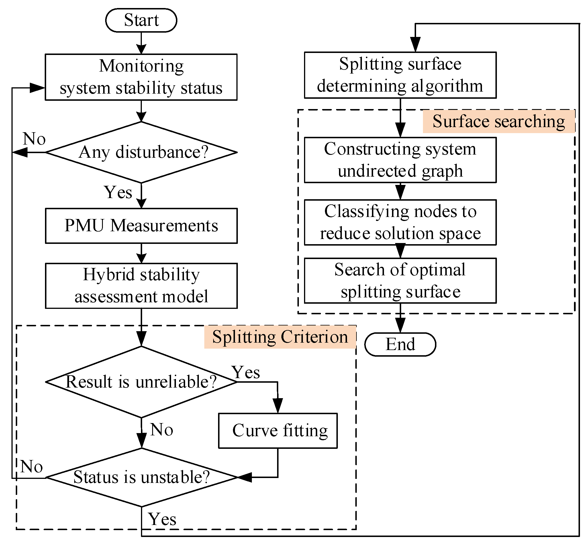
Therefore, the main objective of this paper is to propose a controlled islanding strategy with high efficiency and reliability. For the start-up criterion, a transient stability assessment model aimed at maximizing the benefits of model-free methods is constructed by integrating machine learning and the trajectory fitting (TF) method. Furthermore, an optimal splitting surface determining algorithm based on graph theory is proposed; this algorithm avoids feasible solution loss using the modified network reduction method.

The remainder of this paper is organized as follows: In Section 2, key issues about controlled islanding strategy design is discussed. The transient stability assessment model for the start-up criterion and the searching algorithm for the optimal splitting surface are presented in Section 3 and Section 4, respectively. The implementing structure and process of the proposed controlled islanding strategy is explained in Section 5. Case studies and the conclusions are presented in Section 6 and Section 7, respectively.

2. Controlled Islanding Strategy Design

In contrast with conventional passive islanding, controlled islanding is an online, centralized, and globalized implementation method for system separation. This method determines the splitting locations rapidly with globally obtained operation information and constraints, e.g., power imbalance and power-flow disruption. Hence, controlled islanding always shows outstanding performance.

Determining both when and where to separate the power system is essential for controlled islanding. The splitting action occasion is influential on the dynamics of post-splitting systems. The splitting surface selection determines the operational state of the isolated system and the subsequent control measures.

Regarding the task of “when”, prompt transient stability assessment is an effective tool. Model-based transient stability assessment methods, e.g., time simulation and transient energy function, are restricted by excessive computing time or high complexity in the analysis of a large-scale power system. Machine learning-based methods have been widely applied in stability assessment, exhibiting good performance. Among these machine learning methods, the ELM algorithm has been demonstrated to be useful for transient stability assessment because of its high training efficiency and preferable accuracy. In [19], the ELM was verified to provide incorrect judgments at relatively high possibility, if its output is within a certain interval. This result indicated that the accuracy of the ELM-based transient stability assessment model could be enhanced further with specifical amendments. In this paper, the TF method in [13] is adopted as the enforcement tool for amendments. Hence, the start-up criterion for controlled islanding strategy is determined using a transient stability model constructed based on the ELM and the TF method. The model realizes a balance between computing speed and accuracy through a proposed coordinating mechanism.

Regarding the task of “where”, it aims to determine a suitable islanding surface to ensure the stability of the post-splitting subgroup system. In this paper, “suitable solution” corresponds to the splitting surface with minimal power imbalance and power-flow disruption, where minimal power imbalance is regarded as the objective function in the optimal splitting surface calculation. Theoretically, the searching algorithm requires a large calculation quantity because of the extensive possibility of splitting line sets; this situation is known as a typical NP-hard (non-deterministic polynomial) problem. For either graph theory-based methods or slow coherency theory-based methods, determining the splitting surface is intended to search for generator groups with weak connections. Hence, the possible solution space can be pre-filtered with an evaluation of the electrical connection strength. The electrical distance with line reactance only is such an evaluation index; however, this index’s static feature may lead to loss of feasible solutions in the network reduction. In this paper, a modified electrical distance defined by the ratio of the transmission line reactance and the active power measurements (x_ij/P_ij) is proposed for solution space reduction.

3. Hybrid Transient Stability Assessment Model for Activation Criterion

Conventional passive islanding relies on local electrical information to function. Controlled islanding makes a decision based on global system information, and its action state depends on transient stability assessment results.

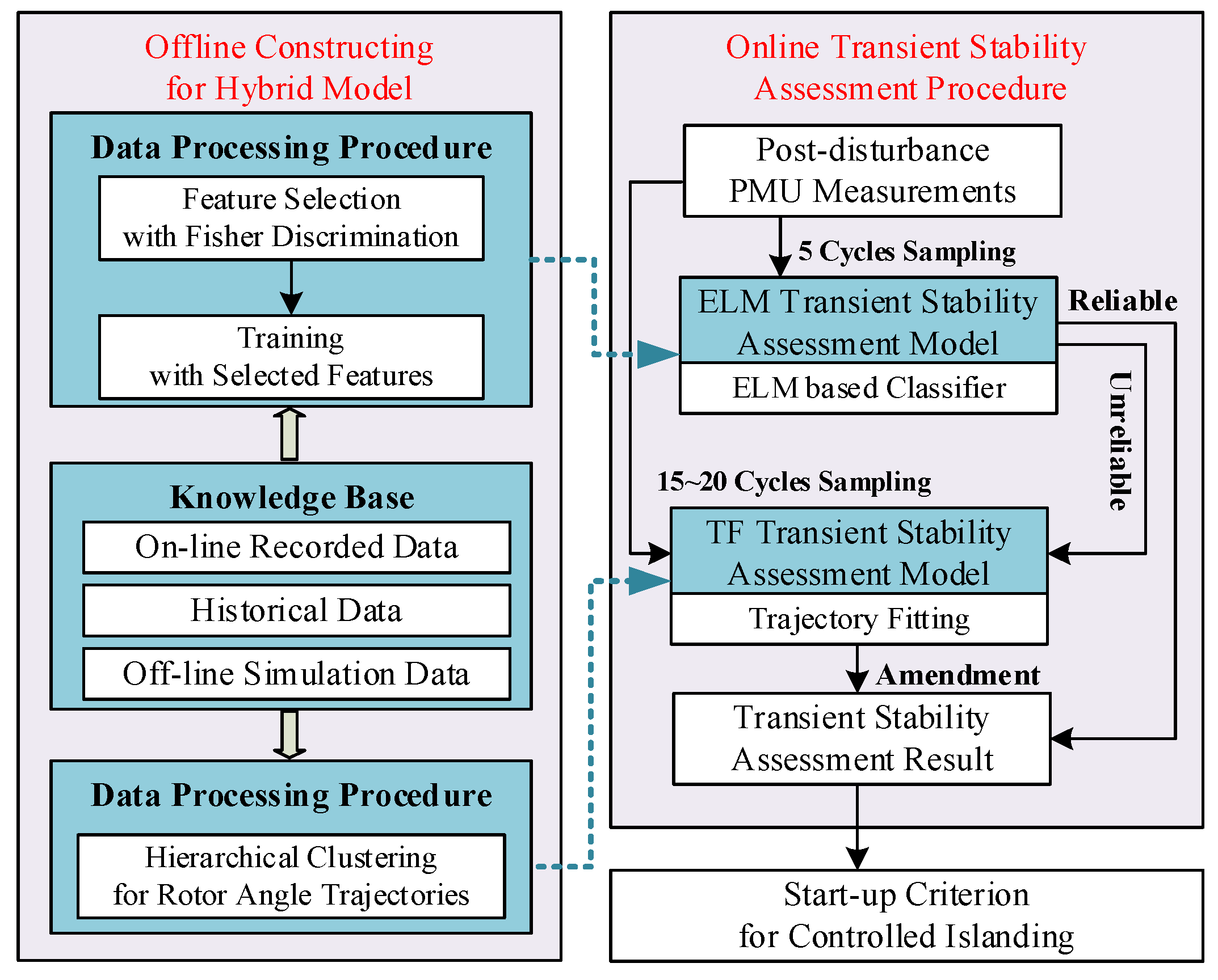
In this part, a hybrid transient stability assessment model based on the ELM and the TF method is constructed, as shown in Figure 1. The proposed model can provide support for making a controlled islanding decision with post-disturbance system stability assessment results. If the assessment result is stable, then subsequent measures for controlled islanding (e.g., splitting surface searching and splitting actions) will not be triggered. Otherwise, the splitting surface searching algorithm will be initiated at once with generator grouping information.

3.1. ELM Theory

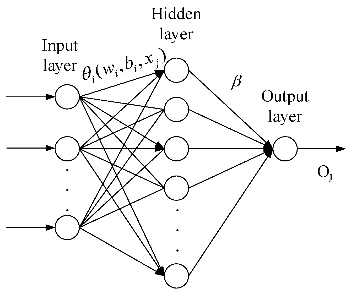
The ELM is a single hidden layer feed-forward neural network algorithm proposed by Huang [29]. Compared with a conventional neural network algorithm, the ELM algorithm determines the parameters of hidden nodes using a random assignment and inverse calculation process, rather than the time-consuming tuning process using the gradient descent method, thereby guaranteeing its high training speed.

Training samples with N sets can be represented as follows:

$${\aleph }_N={\left\{(x_i,t_i)|x_i\in R^n,t_i\in R^m\right\}}_{i=1}^N$$

(1)

where x_i is a n × 1 input vector, and t_i is a m × 1 target vector. A single-hidden layer network with activation function θ(x) can be modeled as:

$${\displaystyle \sum _{i=1}^{\tilde{N}}{\beta }_i{\vartheta }_i(w_i,b_i,x_j)}=o_j,j=1,\dots ,N$$

(2)

where $\tilde{N}$ represents the number of hidden nodes, $w_i={[w_{i1},w_{i2},\dots ,w_{in}]}^T$ and b_i are parameters of the hidden nodes, and ${\beta }_i={[{\beta }_{i1},{\beta }_{i2},\dots ,{\beta }_{in}]}^{\mathrm{T}}$ is the weighting vector connecting the i-th hidden nodes and the output nodes. The structure of the ELM algorithm is shown in Figure 2.

For each training sample, the calculated outputs are expected to remain the same as the actual results, which can be represented as ${\displaystyle \sum _{j=1}^N\Vert o_j-t_j\Vert =0}$. Therefore, ${\beta }_i$, $b_i$, $w_i$ is to be determined to satisfy ${\displaystyle \sum _{i=1}^{\tilde{N}}{\beta }_i{\vartheta }_i(w_i,b_i,x_j)}=t_j,j=1,\dots ,N$, which can be written in matrix form as follows:

$$H\beta =T$$

(3)

where:

$$\begin{gathered} H(w_1,\dots ,w_{\tilde{N}},b_1,\dots ,b_{\tilde{N}},x_1,\dots ,x_{\tilde{N}})={\left[\begin{array}{ccc}\vartheta (w_i,b_i,x_1)& & \vartheta (w_{\tilde{N}},b_{\tilde{N}},x_1)\\ ⋮& \cdots & ⋮\\ \vartheta (w_i,b_i,x_N)& & \vartheta (w_{\tilde{N}},b_{\tilde{N}},x_N)\end{array}\right]}_{N\times \tilde{N}}, \\ \beta ={\left[\begin{array}{c}{\beta }_{{}_1}^{\mathrm{T}}\\ ⋮\\ {\beta }_{\tilde{N}}^{\mathrm{T}}\end{array}\right]}_{\tilde{N}\times m}T={\left[\begin{array}{c}{t}_1^{\mathrm{T}}\\ ⋮\\ t_N^{\mathrm{T}}\end{array}\right]}_{N\times m} \end{gathered}$$

Hence, the training process is to determine β_i, w_i, and b_i. For the ELM training algorithm, the parameters w_i and b_i are fixed before training with random values. β_i is the only undetermined parameter. If the number of hidden neurons is equal to the number of training samples, then β_i can be calculated easily [29]. Although the number of hidden neurons is less than the number of training samples, generally, precise values of β_i, w_i. and b_i, may not exist. The mathematical model can be transformed to minimize the cost function given below, where ${\beta }_i$, $b_i$, $w_i$ (the optimal approximate solution) are to be determined:

$$E={{\displaystyle \sum _{j=1}^N\left({\displaystyle \sum _{i=1}^L{\tilde{\beta }}_i\vartheta ({\tilde{w}}_i\cdot X_j+{\tilde{b}}_i)-t_j}\right)}}^2$$

(4)

For fixed ${\tilde{w}}_i$, ${\tilde{b}}_i$, ${\tilde{\beta }}_i$ the approximate solution can be easily determined [29].

The ELM-based transient stability assessment model is constructed through three main steps. First, historical samples and offline simulation samples, which consist of system features, are collected for feature selection. The recorded actual data can be used to supplement the prior knowledge base to ensure the adaptation to a practical power system. Second, Fisher discrimination is implemented to determine the features that are closely related to the system transient stability status from the initial features with samples in the prior knowledge base. In this manner, the required data scale is reduced and the computing efficiency is improved.

In this paper, the initial features (listed in

Table 1. Initial features for Fisher discrimination evaluation.

Notation	Description
δi	rotor angle variation of generator i
Vi, θi	voltage amplitude and phase angle variation of bus i
Pin,i, Qin,i	active and reactive power injection variation of bus i
PL,i, QL,i	active and reactive power flow of line i
Finfo (ftime and fduration)	fault information (fault time and fault duration)
L, Lnode	load level

) can be obtained by PMU measurements.

Finally, the selected features are regarded as significant features and applied for training of the ELM-based classifier. Once the classifier is established, the ELM transient stability assessment model is constructed. In practical implementation, the transient stability status is judged by the assessment model according to the PMU measurements of the significant features within a short time delay.

3.2. ELM-Based Transient Stability Assessment Model

As mentioned above, the accuracy of a machine learning technique-based method is greatly influenced by the scale and quality of the training samples, as well as the training approach. To improve the accuracy, the TF method [13] is applied to amend the outputs of the ELM-based stability assessment model in certain cases; this approach indicates a coordination mechanism exists in the hybrid transient stability assessment model. The TF method can be constructed using the following two steps:

• Generator rotor angle trajectories in various scenarios are collected from simulation and historical samples and comprise the prior sample database for one certain generator. The difference between samples is measured by the vector distance and is defined as follows:

  $$f(x_{i,T},x_{j,T})={\left({\displaystyle \sum _{t=0}^{T-1}{(x_{i,t}-x_{j,t})}^2}\right)}^{\frac{1}{2}}$$

  (5)

  where x_i,T, x_j,T are samples i and j with data of T moments. The samples are considered approximate if the vector distance between them is less than a certain threshold.
• Approximate trajectory samples are grouped using the hierarchical clustering algorithm. The trajectory having the minimum vector distance with other trajectories is defined as the standard trajectory of the group. Standard trajectories comprise the standard trajectory pattern library, and the measured trajectory is subsequently matched with pattern trajectories in this pattern library to predict the rotor angle trajectory tendency. If the rotor angle of any generator is beyond 180° with the predicted trajectory, then it is judged as a transient instability. Otherwise, it is stable in the transient process.

As the essential component of the hybrid transient stability assessment model, the coordination mechanism is designed for sampling time and result amendment. The ELM- and the TF-based assessment model require five cycles and 15–20 cycles of sampling time, respectively. If the measurements are sufficient in quantity and quality, then the assessment model is initiated immediately. With the conclusion that output of the ELM-based model is problematic in a certain interval in [19], the result amendment procedure is triggered if the output of the ELM-based model is in an unreliable interval. In this case, the TF-based method is used for this amendment procedure and determines the final transient stability assessment result. The determined result is taken as the start-up criterion to decide whether to start up the controlled islanding surface searching algorithm and the splitting action.

4. Optimal Splitting Surface Search Algorithm

The splitting surface searching approach is always used to determine weakly-connected generator groups, among which an out-of-synchronization state typically occurs. In this section, a modified electrical distance index is used to determine those nodes having vague connection with separated generator groups, which could significantly simplify the solution space without feasible solution loss. The ‘optimal’ algorithm involves satisfying some other constraints and considering an active power imbalance of the isolated system as the objective function in the proposed searching algorithm.

4.1. Nodes Classification

Conventionally, a power system is considered to be an undirected graph with edge weight and the accumulated value of the edge weights between nodes is regarded as the electrical distance. In most cases, the reactance of lines is defined as the edge weight for network simplification, and nodes in the electrical network can be divided into two types. Nodes near one certain group of coherent generators in electrical distance are labeled as normal nodes (NN). Otherwise, if nodes share a similar connection with multiple groups of coherent generators, then they are classified as public nodes (PN).

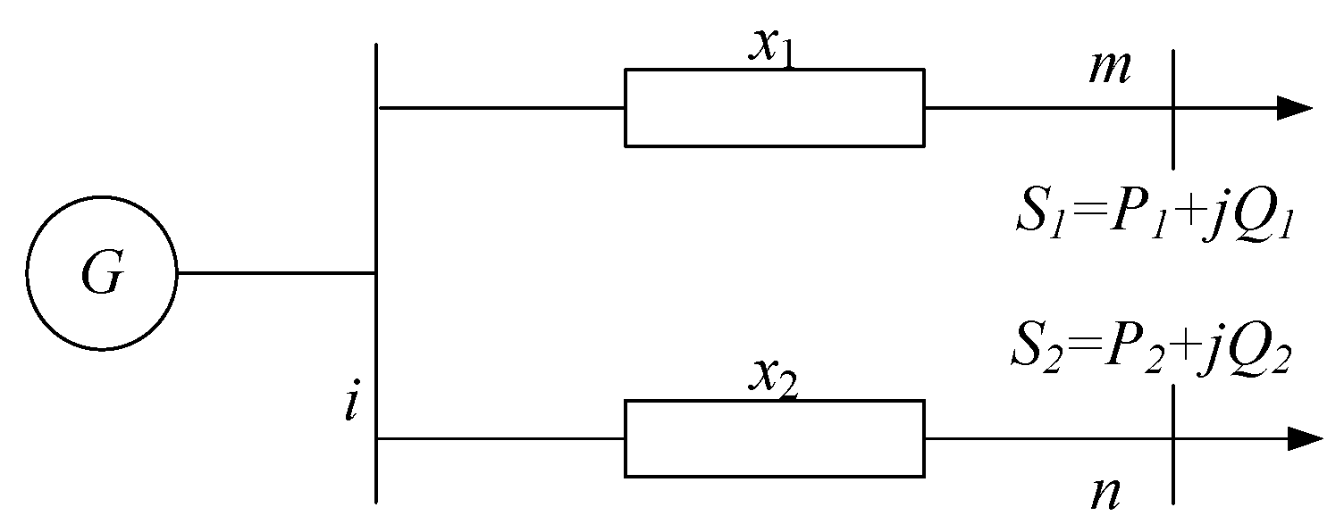
However, considering reactance only in the electrical distance is not complete, theoretically. The detailed analysis of a specific case is shown below:

Figure 3 shows a structure of a simple power system, where the reactance of two lines is equal, i.e., x₁ = x₂, and the load on buses m and n are S₁ = 2S₂, where S₁ = 2S₂, i.e., the active power transmitted between node i and m is twice as much as that between node i and n. Therefore, the electrical distance between nodes i and m is equal to that between nodes i and n when only reactance is considered in the electrical distance. However, this approach neglects the effect of transmitted power on the lines. In this paper, the ratio of the reactance and the active power of the lines is considered as the edge weight to evaluate the electrical distance. We take the IEEE-9 test system as an example to show the advantage of this approach as follows:

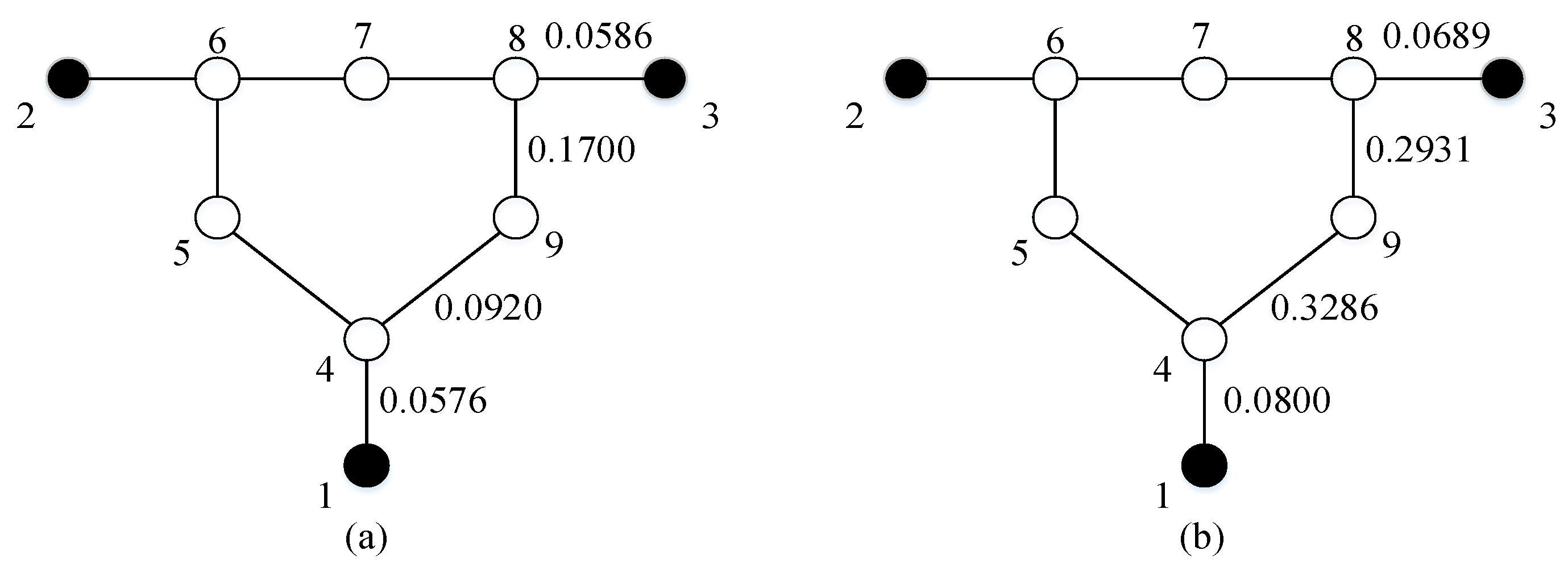
The effect of the edge weight on the results of determining the splitting surface is analyzed on the IEEE-9 test system [25]. Figure 4 shows the edge weight defined with x_ij and x_ij/P_ij of the IEEE-9 test system in (a) and (b), respectively. The minimum accumulating value of the edge weight from node 9 to nodes 1 and 3 are calculated, as summarized in

Table 2. Minimum edge weight cumulative summation.

Edge Weight Definition	Minimum Accumulating Edge Weight Value
	Node 9 to 1	Node 9 to 3
xij	0.1496	0.2286
xij/Pij	0.4086	0.3620

.

Table 2 indicates that edge weight defined with x_ij has smaller weight value from node 9 to 1, i.e., node 9 is closer to node 1 than to node 3. While nodes 9 to 3 have relatively stronger connections for the edge weight defined by x_ij/P_ij. This difference may lead to a loss of feasible solutions in network reduction for the reactance-only scenario. Hence, further research is necessary to consider reactance not only in the electrical distance.

In this paper, x_ij/P_ij is defined as the edge weight of the undirected graph-model. Reduction of the islanding solution space is executed using the following steps:

• Calculating the minimum accumulative edge weight among nodes using the Floyd algorithm. The electrical distance between the load nodes and the coherent generator groups can be written as:

  $$D_{i\to m}=\frac{1}{N_m}{\displaystyle \sum _{j=1}^{N_m}{W}_{ij}}$$

  (6)

  where N_m is the number of generators in coherent group m, and W_ij is the minimum accumulative edge weight between load node i and generator node j in group m.
• The difference in the electrical distance between load node i and two generator groups m1 and m2 can be estimated as:

  $$\gamma =D_{i\to m_1}-D_{i\to m_2}$$

  (7)

A threshold $\epsilon$ is pre-determined according to statistical data and operational experience, with the public nodes occupying approximately 20% of the whole nodes. Node i is defined as the public node of the two generator groups when $\left|\gamma \right|<\epsilon$. If $\left|\gamma \right|>\epsilon$, then node i is defined as a normal node and node i is classified as a closely connected generator group according to the positive-negative value of γ.

4.2. Optimal Splitting Surface Searching Algorithm

On basis of node classification, a normal node is assigned to a corresponding generator group. The essence of searching the optimal splitting surface becomes distribution of the public nodes into suitable generator groups. To determine the optimal splitting surface, the minimum active power imbalance and the minimal power-flow disruption are applied as the objective functions in Equations (8) and (9), respectively:

$$\begin{array}{cc}\min & \Delta P=\left|P_G-P_L\right|\end{array}$$

(8)

$$\begin{array}{cc}\min & {\displaystyle \sum _{i\in V_1,j\in V_2}\left|P_{ij}\right|}\end{array}$$

(9)

where P_G and P_L denote the active power of the generators and the loads in the isolated system respectively, and P_ij is the active power transmitted between nodes i and j. The minimum active power imbalance of the isolated system determines whether the isolated system can recover from load-generation imbalance. Minimum power-flow disruption can reduce the disruption caused by variation of the power-flow dispatch. In this paper, the minimum active power imbalance of the isolated system is taken as the objective function. The set of public nodes is distributed into suitable generator groups using the Breadth First Search (BFS) algorithm for optimal splitting location determination.

5. Controlled Islanding Implementing Strategy

The problems of when and where to separate the power system are solved by implementing the proposed strategy. In this strategy, the splitting action is supposed to be executed once the splitting location is determined by the optimal splitting surface searching algorithm. The implementation of the proposed controlled islanding strategy is shown in Figure 5; the details of the steps are as follows:

Step 1:

Start the prediction program after a disturbance is detected.

Step 2:

Capture the PMU measurements required by the hybrid transient stability assessment model. Note that the sampling time is different for the ELM- and for the TF-based models in this hybrid assessment model.

Step 3:

Initiate the splitting criterion-deciding procedure using the hybrid transient stability assessment model. In this model, the amending procedure using the TF model is activated if the output of the ELM model shows uncertainty.

Step 4:

Judge whether to start the optimal islanding surface searching algorithm according to the splitting criterion, i.e., the system stability status. If the power system tends to lose stability, then go to step 5; otherwise, go to step 1.

Step 5:

The optimal splitting surface searching program starts. Series procedures, including system undirected graph construction, nodes classification, and optimal solution calculating, are conducted.

Step 6:

The optimal splitting surface is determined, and the splitting action is immediately executed. The program ends, and the next round begins.

It can be inferred from Figure 5 that the hybrid transient stability assessment model and the optimal splitting surface searching algorithm are essential parts of the proposed strategy. In the hybrid model, the ELM method output assessment result is taken in most cases and the TF method amendment is taken in certain cases to realize optimization of the combination of computing speed and accuracy. Moreover, the splitting surface with a minimized active power imbalance can be determined rapidly via reduction of the possible solution space. Sequentially, fast and reliable detection of transient instability and determination of the optimal splitting surface is realized, thereby achieving the purpose of the proposed strategy.

6. Case Study

The New England 39-bus test system is used as the testbed for validation of the proposed controlled islanding strategy. To construct the transient stability assessment model, 10,000 samples are generated using the Monte Carlo method; 9000 of these samples are applied for training and trajectory clustering, and the rest are applied for testing. The transient stability status will be determined to be unstable as soon as the rotor angle of any generator exceeds 180° compared with the reference generator.

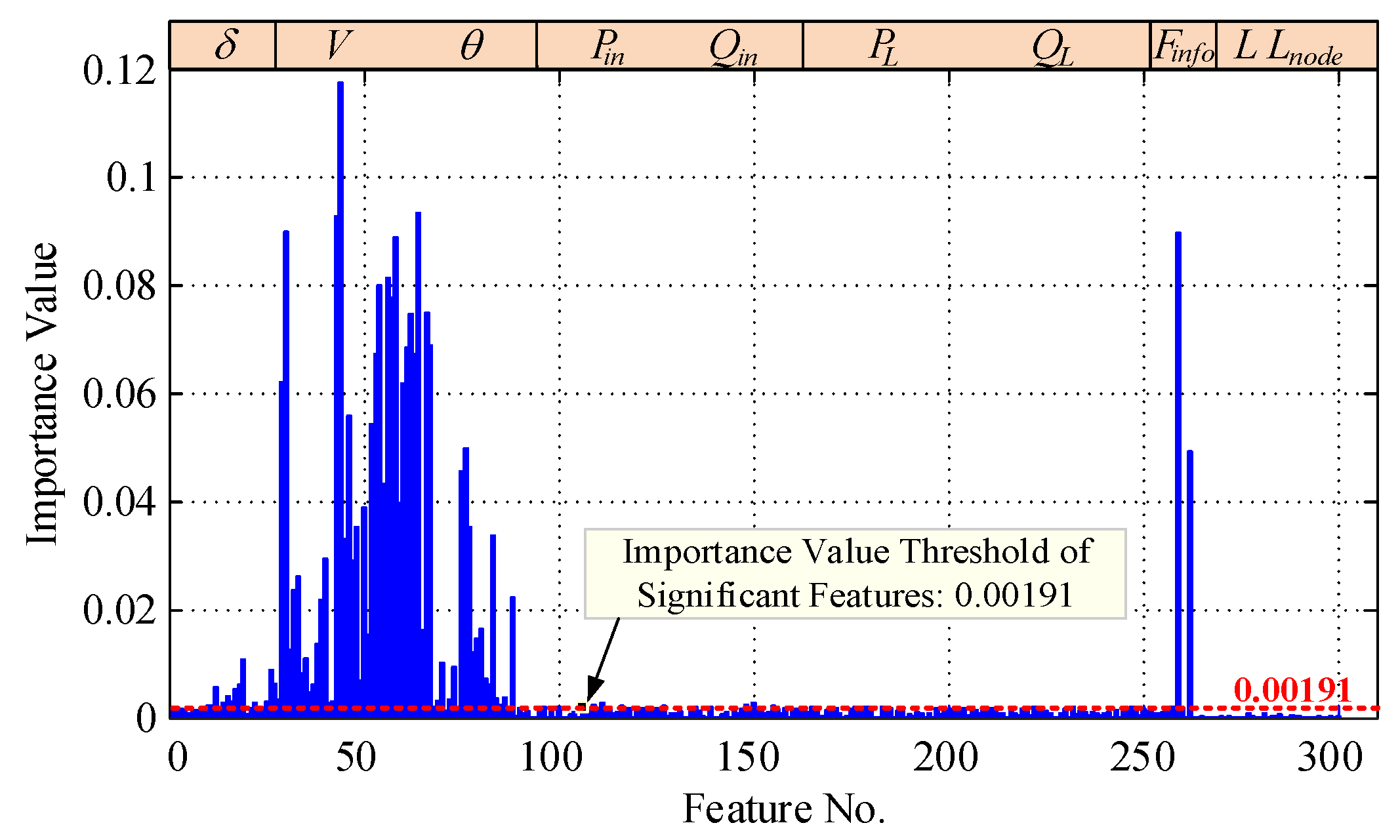
Initial features for feature selection are summarized in Table 1. These initial features are processed via Fisher discrimination to determine the significant features. Figure 6 shows the importance value for each feature, and the top 100 features of the total are chosen as the inputs for the ELM classifier training.

Figure 6 shows that most significant features are dynamic information, e.g., voltage magnitude and phase angle variation, generator rotor angle variation, and fault information. These significant features are used as the ELM training and model inputs. Examinations on the ELM-based transient stability assessment model show that accuracy can reach 97.46% with 1350 hidden nodes at maximum.

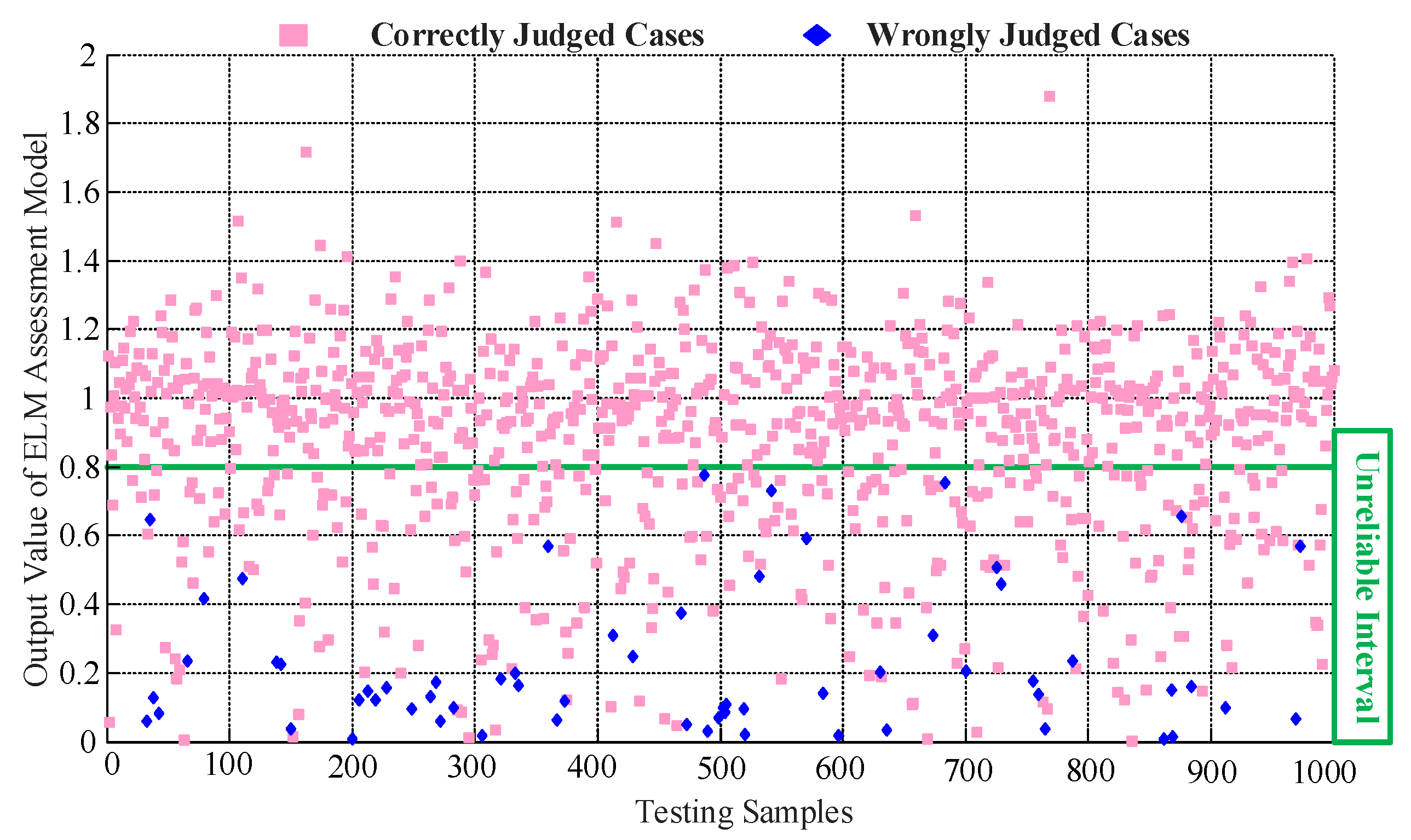
Misjudged cases of the ELM-based transient stability assessment model are small in quantity, but are inevitable. The distribution of the output value for correct and incorrect assessment of the ELM-based model is further studied, as shown in Figure 7.

This finding indicates that the output value for the most misjudged case is within a specific interval ranging from 0 to 1.0, which is defined as the unreliable interval. In this paper, the unreliable interval is set as (0, 0.8).

In the hybrid transient stability assessment model, the TF method is applied to amend the ELM assessment results in the unreliable interval. When number of hidden nodes of the ELM algorithm is set as 500, the accuracy is improved from 94.1% (ELM only model) to 100% (hybrid model). The results show that 355 sets of 1000 test samples with problematic outputs are processed using the TF-based model. The TF method rectifies the ELM-based model assessment results 63 times, 45 of which are corrected from the stable condition to the unstable condition. The expected computing time for each test sample increases from 0.041 s (ELM only model) to 0.136 s (hybrid model). Compared with the ELM-only method, the computing time is a slightly longer, but the accuracy is highly improved.

6.1. Case 1: Assessment by ELM Model is Reliable

In this case, a three-phase short circuit fault is set to occur at 0 s in the middle of lines 23–24 and is cleared at 0.4 s. The generators form two coherent groups: {33, 34, 35, 36} and {30, 31, 32, 37, 38, 39}, in which generators 33–36 are the critical crew. Identification of the instability using the ELM-based transient stability assessment model requires 0.036 s. On the basis of the node classification mentioned above, the evaluation value for the electrical distance between load nodes and two generator groups are listed in

Table 3. Difference of the minimum edge weights cumulative summation.

Nodes	γ	Nodes	γ	Nodes	γ
1	0.0392	11	0.0332	21	−0.0749
2	0.0276	12	0.0318	22	−0.0772
3	0.0221	13	0.0318	23	−0.0859
4	0.0369	14	0.0295	24	−0.0790
5	0.0379	15	-0.0699	25	0.0300
6	0.0372	16	-0.0721	26	0.0442
7	0.0372	17	−0.0663	27	0.0442
8	0.0379	18	−0.0587	28	0.0545
9	0.0547	19	−0.0764	29	0.0551
10	0.0327	20	−0.0803

.

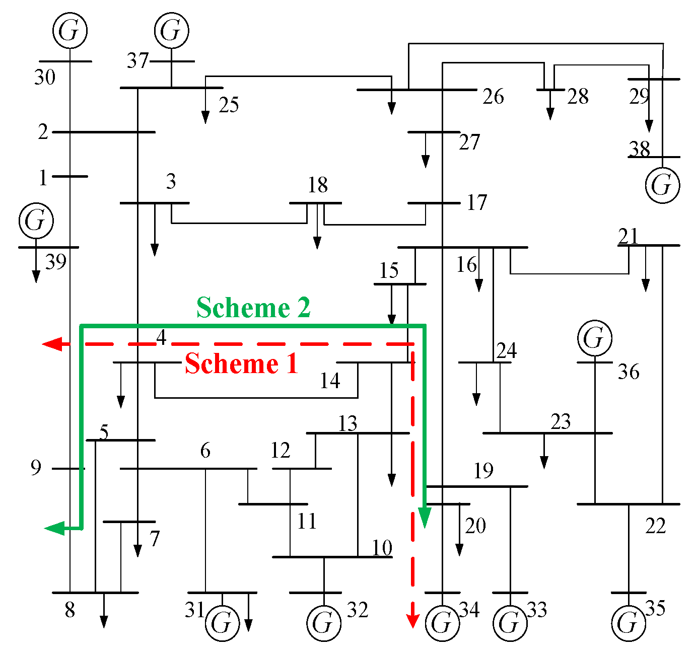
The threshold ε is set as 0.035. Therefore, nodes 2, 3, 10, 11, 12, 13, 14, and 25 are defined as public nodes. Normal nodes 15, 16, 17, 18, 19, 20, 21, 22, 23, and 24 belong to the generator group {33, 34, 35, 36}. The calculated optimal splitting surface solution is shown in Figure 8 with the red dashed line (Scheme 1).

It can be inferred from Table 3 that node 27 has a shorter electrical distance from the generator group {30, 31, 32, 37, 38, 39} than from {33, 34, 35, 36}. In the algorithm defining the reactance as the edge weight, node 27 is classified into the generator group {33, 34, 35, 36}, and the final splitting solution is shown in Figure 8 with the green solid line (Scheme 2). To show the strength of the proposed algorithm, the algorithm defining reactance as the edge weight is contrasted from the aspect of active power imbalance and power-flow disruption in

Table 4. Comparison of the islanding surface searching algorithms.

Islanding Strategy	Active Power Imbalance (p.u.)	Power-Flow Disruption (p.u.)
14–15, 3–18, 17–27	0.329/0.130	0.805
14–15, 17–18, 26–27	0.901/1.360	4.913

.

The table indicates that algorithm considering only reactance in electrical distance may lead to loss of feasible solutions and, thus, affect the final optimal solution. In this condition, power flow disruption is higher than the result found using the proposed algorithm.

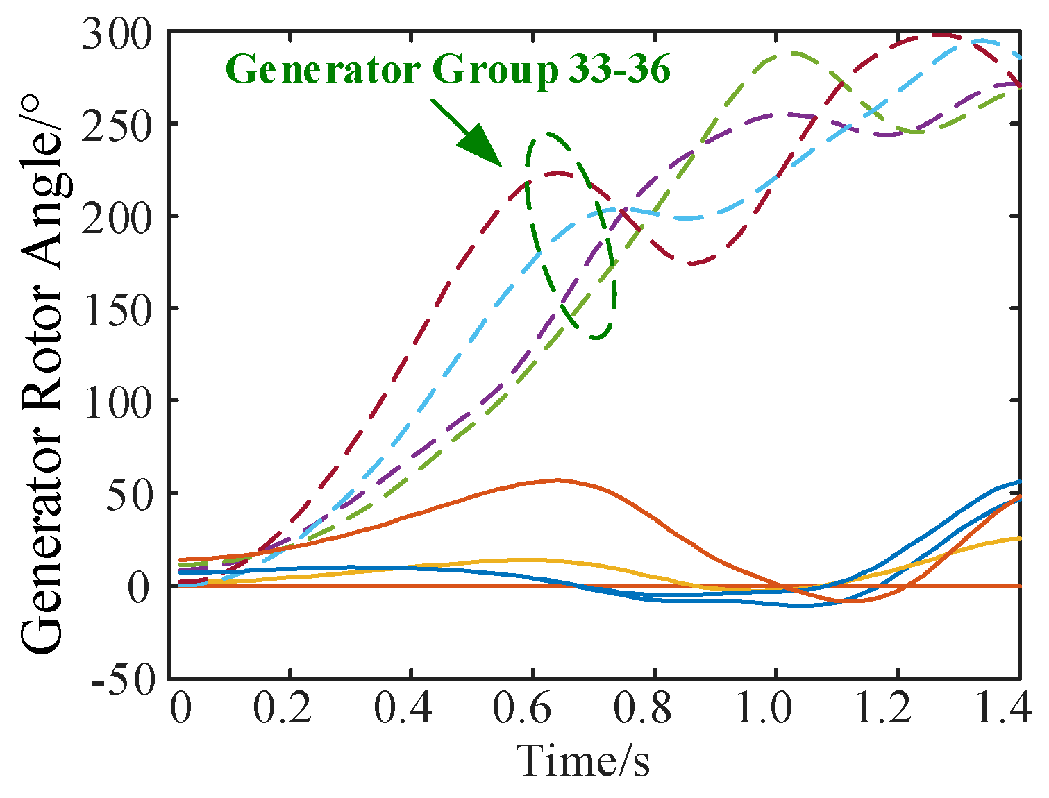
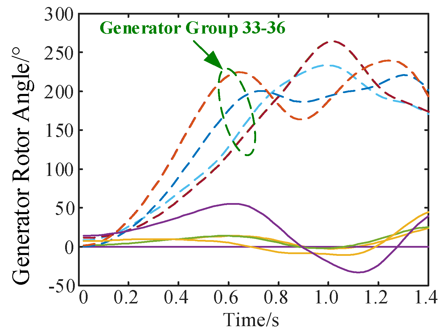
Figure 9 and Figure 10 show the trajectories of the critical generator group {33, 34, 35, 36} using the two islanding strategies. Variation of the generator rotor angle shows that the islanding solution presented in this paper retains system stability better.

6.2. Case 2: ELM Output Located in the Unreliable Interval

In this case, a three-phase short circuit fault occurs at 0.1 s at the middle of line 6–7 and continues for 0.4 s until it is cleared. This fault leads to desynchronization between the generator group {31, 32} and the remaining generators. It takes approximately 0.3 s of computing time to ensure an accurate assessment using the TF method because the ELM output is located in the unreliable interval [0, 0.8].

The optimal splitting solution is shown in Figure 11, marked with the red dashed line (Scheme 1). The solution is contrasted with the results (Scheme 2 in Figure 11) determined by the algorithm presented in the literature [30], whose objective function is the minimum power-flow disruption; a comparison of the results is shown in

Table 5. Comparison of islanding surface searching algorithms.

Islanding Strategy	Power-Flow Disruption (p.u.)	Time (ms)
3–4, 9–39, 14–15	1.2733	≈11
3–4, 8–9, 14–15	1.2678	≈40

.

It is apparent that the algorithm that determines the minimum cut ensures the minimum power-flow disruption. Compared with this algorithm, the proposed algorithm in this paper can also avoid high power-flow disruption by taking active power on transmission lines into consideration in the concept of the electrical distance. Using the proposed algorithm, the solution space is reduced based on the electrical distance, resulting in a reduced computing time while providing a consistent (nearly identical) result.

The validation results illustrate that the ELM-based transient stability assessment model is computationally efficient. The TF method is able to amend the problematic results of the ELM-based assessment model; however, this amendment requires a slightly longer computing time. The algorithm proposed for optimal splitting location determination reduces the solution space using the modified electrical distance concept while not losing any feasible solutions.

7. Conclusions

In this paper, a controlled islanding strategy consisting of prompt transient stability assessment and optimal splitting surface determination was described.

(1).

A hybrid transient stability assessment model based on the ELM and TF methods was constructed to determine the start-up criterion. In this model, the ELM method is used for prompt stability assessment, and the TF method is employed to enhance the reliability of the assessment results.

(2).

A rapid algorithm comprised of network reduction and optimal solution searching was proposed to determine the splitting surface. In this algorithm, feasible solution loss in the network reduction process is avoided by modifying the evaluation index of the electrical distance.

Using the proposed method, both the start-up criterion and the optimal splitting surface can be determined online with high reliability. The results showed that the proposed controlled islanding strategy is effective in preventing transient instability. As the scenarios considered in this work were designed optimally, the sample generation problem and data acquisition risks in a realistic scenario were ignored. Further research can be dedicated to these problems to achieve reliable performance of the proposed controlled islanding strategy in a practical implementation.