Abstract
This study investigates a demand-side management problem in which multiple suppliers compete with each other to maximize their own revenue. We consider that suppliers have heterogeneous energy sources and individually set the unit price of each energy source. Then, consumers that share a net utility react to the suppliers’ decisions on prices by deciding the amount of energy to request, or how to split the consumers’ aggregated demand over multiple suppliers. In this case, the consumers need to consider the power loss and the price to pay for procuring electricity. We analyze the economic benefits of such a pricing competition among suppliers (e.g., a demand-side management that considers consumers’ reaction). This is achieved by designing a hierarchical decision-making scheme as a multileader–multifollower Stackelberg game. We show that the behaviors of both consumers and suppliers based on well-designed utility functions converge to a unique equilibrium solution. This allows them to maximize the payoff from all participating consumers and suppliers. Accordingly, closed-form expressions are provided for the corresponding strategies of the consumers and the suppliers. Finally, we provide numerical examples to illustrate the effectiveness of the solutions. This game-theoretic study provides an example of incentives and insight for demand-side management in future power grids.
1. Introduction
Due to the growing concerns over environmental damage from existing power grids and the depletion of traditional fossil fuel sources, next-generation power grids are envisioned to transform traditional power grids into more energy-efficient, reliable, and responsive systems [1,2,3]. This evolution can be achieved by integrating modern communication technologies and innovations in distributed generation from renewable energy sources. Such systems are known as [4,5,6]. Balancing demand and supply in a smartgrid has proved to be a challenge because of the highly variable, unpredictable, and intermittent nature of energy generation from renewable sources [4].
Demand-side management (DSM) is a promising responsive system for smartgrids to manage consumer demand [7,8,9,10,11,12,13,14,15]. For instance, a supplier can directly manage its consumer demand to maximize its revenue or improve energy efficiency. This is generally based on an agreement between suppliers and consumers. However, a major drawback of this approach is related to concerns regarding consumer privacy issues. Hence, to address these issues, there is an alternative approach wherein suppliers indirectly manage consumer demand by changing energy unit prices over time. This is called a mechanism. Consumers are encouraged to voluntarily manage their demand based on pricing information determined by suppliers [9]. Accordingly, the pricing mechanism impacts both suppliers’ revenues and consumers’ satisfaction [16,17].
This concern has motivated studies to determine the optimal behavior of consumers or to set optimal energy unit prices for DSM. The common goal of these studies is to find optimal strategies for consumers or suppliers by considering the impact of pricing mechanisms [3,12,17,18,19,20,21,22,23,24]. In [10], the authors suggested a DSM strategy that uses a day-ahead load shifting technique to overcome both peak load demand problems. The work of Song [24] proposed an optimal critical peak pricing scheme for DSM by considering the interactions of consumers where there is a single utility company. In this work, a repeated game framework for nonstationary DSM was proposed to minimize the long-term total cost and discomfort cost of consumers. Further, for the practical use of real-time data, the reference [25] suggested a game theoretic model predictive control approach to solve the day-ahead optimization problem while considering forecasting errors. The approach presented in [12] found the optimal behavior of consumers by considering competition among them, and interactions between consumers and a supplier. In this system, a single supplier sets an optimal unit price to maximize its profit. Consumers then individually determine their optimal demand by competing against one another. Recently, in reference [3], the decision processes for both multiple suppliers and consumers were modeled with the intervention of a utility company as an intermediate node. This work assumed that a utility company sets the optimal energy unit price instead of the suppliers, and pricing competition among suppliers was not considered. An incentive-based demand response model proposed by Yu et al. [26] aimed to model three hierarchical levels of a grid operator, multiple suppliers and corresponding consumers. Here, because it is assumed that each supplier serves enrolled consumers, pricing competition among multiple suppliers was not considered. Maharjan et al. [27] applied the Stackelberg game theory and developed a distributed algorithm to find optimal strategies for multiple suppliers and consumers. In their study, each consumer attempted to maximize the logarithmic satisfaction function according to procured energy within pre-defined budgets. However, there was no consideration of the amount of required energy demand, so the required energy level was not guaranteed. Similar to [27], the work of Alshehri [28] is the closest to this study. The authors added the minimum required energy demand as a constraint in the model of [27]. However, there was no consideration of a power loss penalty between multiple suppliers and consumers. In addition, it is difficult to determine efficient budget requirements to meet the minimum required energy demand.
This study addresses a DSM problem in which multiple suppliers conduct pricing competition to maximize their own revenue. We consider that suppliers have heterogeneous energy sources and individually set the unit price of each energy source. Then, consumers that share a common utility cooperatively react by making decisions on how to request (or how to split) the aggregated demand over multiple suppliers to maximize their net utility. It should be noted that all previous research adopted budget requirement and did not consider power loss for electricity transmission between suppliers and consumers. In contrast, in the model proposed here, we consider two penalty terms—namely, power loss and price to procure electricity—in the consumers’ objective function, where the required demand is considered as a constraint. Thus, in the proposed model, setting the budget requirement is not necessary, and consumers can consider both the distance to suppliers and the energy price for the optimal decision. Accordingly, interactions between suppliers and consumers are considered. We analyze the economic benefits of such a pricing competition among suppliers in terms of the DSM problem by considering interactions between suppliers and consumers, which is modeled by a multileader–multifollower Stackelberg game. We show that the behaviors of both consumers and suppliers based on well-designed utility functions converge to a unique equilibrium solution to maximize the payoff for all participating consumers and suppliers. Accordingly, closed-form expressions are provided for the corresponding strategies of both the consumers and the suppliers. Thus, our model accounts for situations in which consumers suffer from a trade-off between power loss and the price of heterogeneous energy sources for DSM.
The contributions of this study are summarized as follows:
- We design the suppliers’ utility function by compromising between both revenue and power generation cost. In addition, the net utility function of procuring electricity for consumers (which represents social welfare for consumers) is well designed by considering the following aspects. (1) the satisfaction from electricity, (2) two penalty terms of power loss and the price to pay for procuring electricity. Accordingly, compared with other studies, setting the budget requirement is not necessary, and consumers determine an optimal strategy by considering both power loss to suppliers and energy price.
- Based on the proposed utility function of the consumer and supplier sides, this study addresses the joint pricing and DSM problem over heterogeneous energy sources in a competitive electric energy market. The problem is formulated as a Stackelberg game (multipleleader-multifollower).
- In the formulated Stackelberg game, we propose a novel DSM scheme for finding the best response of consumers while supporting aggregated demand. On the supplier side, we design a non-cooperative pricing game between multiple suppliers by considering consumers’ reactions. Here, we prove the existence of a Nash equilibrium (NE) in the proposed scenarios.
- With the relaxation of constraints on the DSM problem, closed-form solutions to the proposed problem for both consumers and suppliers are provided. We also prove that a unique Stackelberg equilibrium (SE) exists in the proposed Stackelberg game by providing a gradient iteration algorithm for the SE, based on the mathematical background. In the numerical results, obtained with varying parameters, we analyze the relationship of the best response between consumers and suppliers. The proposed schemes converge well to equilibrium points.
The remainder of this paper is organized as follows. We explain the detailed system model and utility functions for suppliers and consumers in Section 2. In Section 3, the problem is formulated as a Stackelberg game and the SE is discussed. In Section 4, a detailed theoretical analysis of the Stackelberg game is conducted by providing the closed-form solutions and showing the uniqueness of the SE. Finally, we present the numerical results and conclude the work in Section 5 and Section 6, respectively.
2. Competitive Electric Power Market Model with Heterogeneous Power Generators
In this section, we address the problem of a DSM where multiple suppliers compete against one another to maximize their own revenue (Figure 1). We consider a set of suppliers = {1, 2, …, I} who own various heterogeneous power generators (i.e., heterogeneous energy sources). Suppose there are J types of power generators (e.g., thermal energy, solar energy, and wind turbines) in the power grid infrastructures so that we can define the set of power generators with a given supplier i as = {, , …, }. The available power generation capacity of each power generator can be expressed as , with the available power generation capacity of supplier i over the power generator j. Here, a supplier can provide the available power to consumers who are willing to use the power at a given price . In this case, a supplier uses a dedicated control channel to broadcast the availability of power with the payment price to obtain this power. Here, we assume that the consumers are in the same geographical areas. It is a reasonable assumption when only focusing on the population of certain areas. Thus, the consumers can request electric power from all available power generators in of suppliers in simultaneously at every time slot, where there are periodical electric power requests within a given time slot. That is, consumers can procure aggregated electric power from different power generators. In this sense, there is a broker between the suppliers and the consumers who aggregates demand from all consumers and makes demand requests to suppliers based on the consumers’ decisions. It should be noted that the broker concept is widely used in electric power market models to manage energy distribution, as in [4,5]. Here, the total amount of requested demand required to support the whole population is denoted by . To simplify analysis, we also assume that each consumer requests the same amount of power for their own objective (or service) and is willing to cooperate with others to maximize net utility (i.e., social welfare). This means that their optimal demand vector over the provided power generators would all be in the same ratio. Furthermore, the total aggregated demand over all energy sources is , where is the allocated demand vector over the power generator j of supplier i. Thus, the total aggregated demand over all power generators would meet the to support the requested demand.
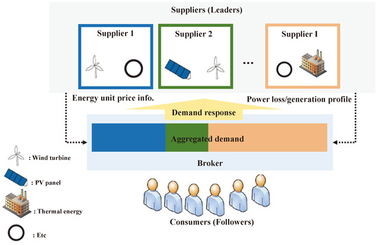
Figure 1.
Stackelberg game model. PV: photovoltaic.
2.1. The Net Utility Function of Consumers (Social Welfare)
Generally, consumers can adaptively control the aggregated demand over the various power generators from the suppliers by simultaneously utilizing available heterogeneous power generators. Based on this assumption, consumers will maximize their net utility—which is coupled with the power loss cost and price to pay—through cooperation, while meeting the requested demand for the whole population. From the consumers’ point of view, total net utility (or social welfare) for the requested demand needs to be modeled using the power loss penalty and the payment price to procure energy. First, we consider the cost of power loss.
- Power loss model: In the power loss model, we consider a general power loss penalty model from [2,29]. Here, the power loss occurs during a power exchange between the consumer and power generator. It is a function of several factors, such as the distance between consumer and power generator, power transfer voltage, and amount of power. In this case, we assume that the power demand vector is less than the available power generation capacity. Thus, the power loss penalty function () is expressed as follows:where V is the transfer voltage, is the resistance of the distribution line between the power generator j of the supplier i and consumers, and is the fraction of power lost in the transformer at generation.
- Proposed net utility function: Therefore, the proposed utility function—which represents the net utility or social welfare—for consumers is presented as follows:where and are the weight factors (≥ 0) for satisfaction of consumers from procuring electricity and payment, respectively. The logarithm term is the consumers’ gain from satisfaction in using a certain amount of electricity. Note that a logarithmic utility function is generally utilized to measure user’s satisfaction with diminishing returns [4,5,6]. In this study, the total requested demand for electricity is defined as a constant. This term should be considered a constant gain term. There are two major motivations for using this utility function. First, because the function is concave, it guarantees the existence of a global optimal point. Second, the adjustable parameters and provide flexibility to fit the function with different priorities for consumers’ satisfaction and payment, respectively.
Proposition 1.
The net utility function of consumers is concave in d.
Proof of Proposition 1.
To prove the concavity of the multi-variable function, we must verify the negative semi-definiteness of the Hessian matrix [30]. If a Hessian of is negative semidefinite for all d, then is concave. The Hessian of is expressed as , , and , where
Consequently, the negative diagonal implies concavity. ☐
2.2. The Supplier’s Utility Function
From the suppliers’ point of view, the total utility function needs to be modeled using the generation cost and total revenue from consumers. Therefore, a novel utility function (i.e., net revenue) from supplier i is presented as follows:
where denotes the cost for generating and operating power generator j to supplier i.
3. A Game-Theoretic Approach: Stackelberg Game
In this section, we introduce a game-theoretic approach to analyze our system model. More specifically, we describe a basic overview of the Stackelberg game and formulate the joint pricing and DSM problem based on the proposed utility functions defined in the previous section.
3.1. Preliminaries
Stackelberg games are a special type of noncooperative game in which there exists a hierarchy among players. For instance, for a two-level game, players can be classified as leaders and followers. In the original work of H. von Stackelberg, the Stackelberg model was designed to analyze a strategic game in economics in which the leader firm moves first and then follower firms move sequentially. This is the case with one single leader and multiple followers. Generally, in a Stackelberg game, each player is assumed to be selfish and rational, and each aims to maximize its utility or revenue. Moreover, the leaders are in a strong position to enforce their strategies on the followers. Hence, in this leader–follower competition, the leaders decide their strategies prior to decision of the followers’ strategies. Therefore, the followers can observe the strategies of the leaders and adapt their own strategies accordingly. In particular, because each follower has the information of the strategy adopted by each leader, they will choose their best strategy (also known as the best response), given the strategies of the leaders. On the other hand, the leaders are aware of the fact that each follower will choose its best response to the leaders’ strategies. Therefore, the leaders are able to maximize their utilities based on the best responses of the followers. The solution of the game is known as the Stackelberg equilibrium. The Stackelberg game approach has advantages for identifying hierarchical equilibrium solutions in this noncooperative decision problem and analyzing the economic benefits [4,5].
In our system model, there are two levels of game where multiple suppliers and multiple consumers exist (Figure 1). The competition game in the first level is among suppliers to sell their electricity to consumers. Here, suppliers take the role of leaders. Each supplier sets its own pricing strategy c to impose price on consumers who demand electricity. Here, multiple leaders hold a strong position, and leaders can impose their own strategy. In the second level, there are other players called followers who react to the leaders’ strategy. The followers—consumers in this case—determine the demand vector over each power generator based on the leaders’ strategy to maximize their net utility through cooperation.
3.2. Novel DSM Scheme at Consumer Side
In the proposed game formulation on the follower side, c is decided by electricity suppliers (i.e., multiple leaders). The followers (i.e., consumers) maximize their own net utility () by performing DSM. That is, they determine the amount of demand to request from the distributed generators while guaranteeing support for the required power demand. Therefore, for a given pricing strategy from the suppliers, we define the best response function for the follower as
where denotes a set of possible demand distribution strategies. To identify the best-response demand-distribution for a given price, we transform Equation (3) into a convex optimization problem. Because the consumers’ net utility function is a concave function, solving the best-response function for a consumer in Equation (3) could be considered a convex optimization problem as follows:
The objective function of Problem (4) is concave, and the problem has linear constraints. Therefore, the problem is a convex optimization problem, which also makes a local maximum the global maximum [31]. The basic principle in Lagrange duality is to relax the original problem (4)–(7) by transferring the constraints to the objective in the form of a weighted sum. We then define a Lagrangian associated with the above problem as:
where is the Lagrange multiplier corresponding to the demand requirement of Equation (5), and = (: ) and = (: ) are vectors of Lagrange multipliers corresponding to the feasible region of the d vector from Equations (6)–(7) with , ≥ 0. Then, the dual function can be expressed as
Accordingly, the dual problem corresponding to the primal problem of Equations (4)–(7) is
Because the primary problem of Equations (4)–(7) is a convex optimization problem, a strong duality exists. The optimal values for the primal and dual problems are equal. As a result, it is appropriate to solve the primal problem through its dual problem of Equation (10). Hence, the optimal power distribution for a fixed value of dual variables (, and ) can be calculated by applying the Karush–Kuhn–Tucker (KKT) conditions on Equation (10). We then obtain:
Using the utility function (1), we conclude that the optimal demand distribution vector is . Therefore, the optimal solution can be calculated as
Here, a gradient descent method can be applied to calculate the optimum values for dual variables (, and ) to solve Equation (12), as given by
where t is the time index of iteration, with s = {1, 2, 3} is a sufficiently small fixed step size, and the notation denotes the projection onto nonnegative orthants [31,32]. Convergence towards the optimum solution is guaranteed because the gradient of Equation (12) satisfies the Lipschitz continuity condition [33]. Specifically, by updating dual variables to a gradient direction [31], the dual variables , , and will converge to the dual optimal , , and , respectively, as , and the solution to Equation (12) will also converge to the optimal . The proposed decomposition method for the optimization problem (4)–(7) is summarized as follows:
3.3. Novel Competitive Pricing Scheme at Supplier Side
Here, we analyze the leaders’ strategies for the Stackelberg game. In this case, we assume that there are multiple leaders (i.e., various suppliers) in the area where consumers can request electric power, and suppliers compete with each other to maximize their own utility. This is accomplished by selecting their pricing strategy based on considering the followers’ best-response. Here, the optimal pricing strategy could be expressed as
where ={, , …, }.
However, the utility function of the leader not only depends on its own strategy, but also on the rate at which it is allocated by the followers as determined in Equation (3). Thus, Equation (16) can be rewritten more specifically,
Therefore, the leader needs to consider the followers’ best-response to the imposed pricing strategy to identify on an optimal strategy. Furthermore, we also consider that multiple leaders compete with each other by setting their own prices. Thus, other suppliers’ strategies are another criterion for deciding one’s own strategy.
Proposition 2.
The DSM algorithm for the follower side (Algorithm 1) is quasi-convex in when other prices () are fixed.
Proof of Proposition 2.
When is gradually increased from zero, the demand distribution will remain equal or decrease. Subsequently, when continues to increase to an infinite value, will reach the value max (0, ). Therefore, the DSM algorithm for the follower side is a non-increasing function in . From [34], a function that is always non-increasing or non-decreasing is quasi-convex; therefore, we can prove that the DSM algorithm for the follower side (Algorithm 1) is quasi-convex in . ☐
| Algorithm 1 A gradient algorithm for demand-side management (DSM). |
|
Based on these perspectives, we prove the existence of NE in this competitive pricing game and SE in the two-level (consumer–supplier) game, respectively. This allows us to provide a gradient algorithm for the SE as represented in Algorithm 2.
Definition 1.
A pricing vector is a Nash equilibrium of the non-cooperative competitive pricing game if, for every i and j, (, ) ≥ (, ) for all ∈, where (, ) is the resulting pricing strategy for the power generator j for the supplier i, given the other power generator pricing results .
Theorem 1.
There exists at least one Nash equilibrium in the non-cooperative competitive pricing game.
Proof.
Note that the strategy is a nonempty, convex, and compact subset of some Euclidean space . The utility function (c) is a non-decreasing function in . The DSM algorithm on the follower side represents a continuous function of demand distribution which is quasi-convex in each from Proposition 2. Therefore, according to [35], the game has at least one NE. ☐
3.4. Existence of Stackelberg Equilibrium
For the formulated Stackelberg game, a pair consisting of leaders’ and followers’ strategies ((= ,… , etc.), ) is called SE if
and . To find the SE, we first solve the best-response function (3) to identify the relationship between the leaders’ and followers’ strategies. Based on that relationship, we can obtain an optimal pricing strategy by solving (18) and determining the SE point(s).
Corollary 1.
At least one Stackelberg equilibrium exists in the proposed two-level game.
Proof of Corollary 1.
There is a unique optimal demand distribution point at the follower level. Correspondingly, there exists at least one NE in the non-cooperative competitive pricing game at the leader level, as shown in Theorem 1. Therefore, the proposed two-level game has at least one SE. ☐
We can use the following gradient-based iteration algorithm to obtain the SE.
| Algorithm 2 Gradient algorithm for Stackelberg equilibrium. |
Input: randomly given a price over energy source j by supplier i 2: Output: optimal demand distribution vector and pricing vector over power generator j by supplier i Repeat the iteration (a) The consumers perform DSM Algorithm 1 to obtain the optimal demand distribution (b) The suppliers update the prices: (c) Until ≤ 4: End iteration |
In Algorithm 1, is the iterative step size of the price, = {, ,…,}, is the gradient with .
4. Theoretical Analysis of the Proposed Stackelberg Game
In this section, we theoretically analyze the proposed Stackeberg game. This is accomplished by providing a closed-form solution with a relaxation of the constraints for the DSM problem. Furthermore, we also prove that a unique SE exists in the proposed two-level game.
4.1. Closed-Form Solution for DSM at the Consumer Side
To find the closed-form solution for theoretical analysis, we assumed that optimal demand distribution is always positive and satisfies the capacity requirements of the power generator under a certain condition of . Hence, inequality constraints (6)–(7) for the optimization problem for DSM are removed. We then redefine the Lagrangian form as follows:
where is the Lagrange multiplier.
To solve the problem, the necessary and sufficient conditions for optimality are then given by the KKT conditions:
Therefore, from Equations (20) and (21), for a given minimum required demand (), the optimal demand distribution at power generator j of supplier i can be obtained as follows:
where X = .
Here, to satisfy the positivity and capacity requirement of optimal demand distribution, we assumed that any positive weight factor should satisfy the condition below, when prices and other constant values are given.
Proposition 3.
The optimal demand distribution at power generator j of supplier i decreases with its prices when other prices are fixed.
Proof of Proposition 3.
Taking the first-order derivative of , we have
Because and are positive and negative, respectively, implies that is decreasing with . ☐
4.2. Closed-Form Solution for Competitive Pricing at the Supplier Side
Here, based on the analytical result (i.e., the closed-form solution) for the DSM for the consumers’ side, we determine that there is a unique SE in the proposed two-level game between consumer and supplier. The leader of the Stackelberg game (the supplier) can optimize its strategy () to maximize its utility as defined in Equation (2), which forms a non-cooperative competitive pricing game. Thus, from Equation (17), the best response from the supplier could be rewritten as
where and are, respectively, the pricing strategy of supplier i for power generator j and all other pricing strategies, except . In addition, is the optimal demand distribution vector for consumers with given pricing c of suppliers.
This can be written as
and we denote the solution of the best response as .
Proposition 4.
The utility function of supplier i is concave in its own price , when the other suppliers’ prices are fixed and optimal demand is allocated by consumers.
Proof of Proposition 4.
Taking the second-order derivative of , we have
Because and are positive and negative, respectively, is less than 0. Therefore, is concave with respect to . ☐
Here, we assume that the cost for generating and operating electricity should be decided such that > 0, given that the variables are constant. Next, we can prove that the supplier-level game has a unique NE; this NE provides a set of prices such that none of the suppliers can increase their individual utility by choosing a different price based on prices offered by other suppliers. The key aspect of the uniqueness proof is to realize that the best response function in Equation (26) is a standard function [35]. A function is said to be standard if it satisfies the following properties:
- positivity: ()> 0;
- monotonicity; if ≥ ,() ≥ ();
- scalability: () > (), ;
Theorem 2.
An arbitrary supplier i’s best response function () is standard. Thus, a unique NE exists in the non-cooperative competitive pricing game between suppliers.
Proof of Theorem 2.
Please find the proof of this theorem in the Appendix A. ☐
4.3. Existence and Uniqueness of Stackelberg Equilibrium (SE) for the Proposed Two-Level Game
For a Stackelberg game, the existence and uniqueness of a SE are two desirable properties. In this subsection, we will prove that solutions and (i∈, j∈) are in SE for the proposed game.
Corollary 2.
A unique Stackelberg equilibrium exists in the proposed two-level game.
Proof of Corollary 2.
Because an arbitrary supplier i’s best response function is standard from Theorem 2, the supplier’s pricing game has a unique NE; therefore, the proposed game also has a unique NE. ☐
5. Numerical Results
In this section, various numerical examples—which were simulated by MATLAB—are presented to verify the proposed theorems and propositions and to investigate the utility of both consumers and suppliers with respect to varying parameters. Therefore, we assumed the following scenario: two different types of power generators (indexed as 1 and 2) with different operating costs o = [, ] = [0.1, 0.2] kW.p.u. and available power generation capacity vectors g = [, ] = [6500, 5000] kW. In addition, the total amount of requested demand required to support the whole population was 4200 kW, and it was assumed to be constant during 1 h. The losses due to resistance between the power generator and consumers and in the transformer were set, respectively, to typical values of = 0.2 ohm per km, = 500, and = 0.02. We also assumed that the distance from power generators 1 and 2 to consumers were 20 km and 10 km, respectively. The voltage V was set to 50 kV, which is a practical value in a variety of smart grid distribution networks [29,36].
5.1. DSM According to Suppliers’ Electric Power Price
We then verify the effect of the electric power price offered by supplier 2 on the demand distribution to suppliers 1 and 2. Figure 2 shows that the demand distribution to supplier 2 linearly decreases with price while is fixed. Conversely, the demand distribution to supplier 1 correspondingly increases by guaranteeing . This intuitive result regarding demand distribution versus price is based on Proposition 3.
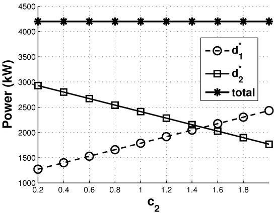
Figure 2.
The demand distribution to suppliers 1 and 2 ( = 0.016) as the price offered by supplier 2 varies.
5.2. Utility of Suppliers and Net Utility of Consumers According to the Suppliers’ Price
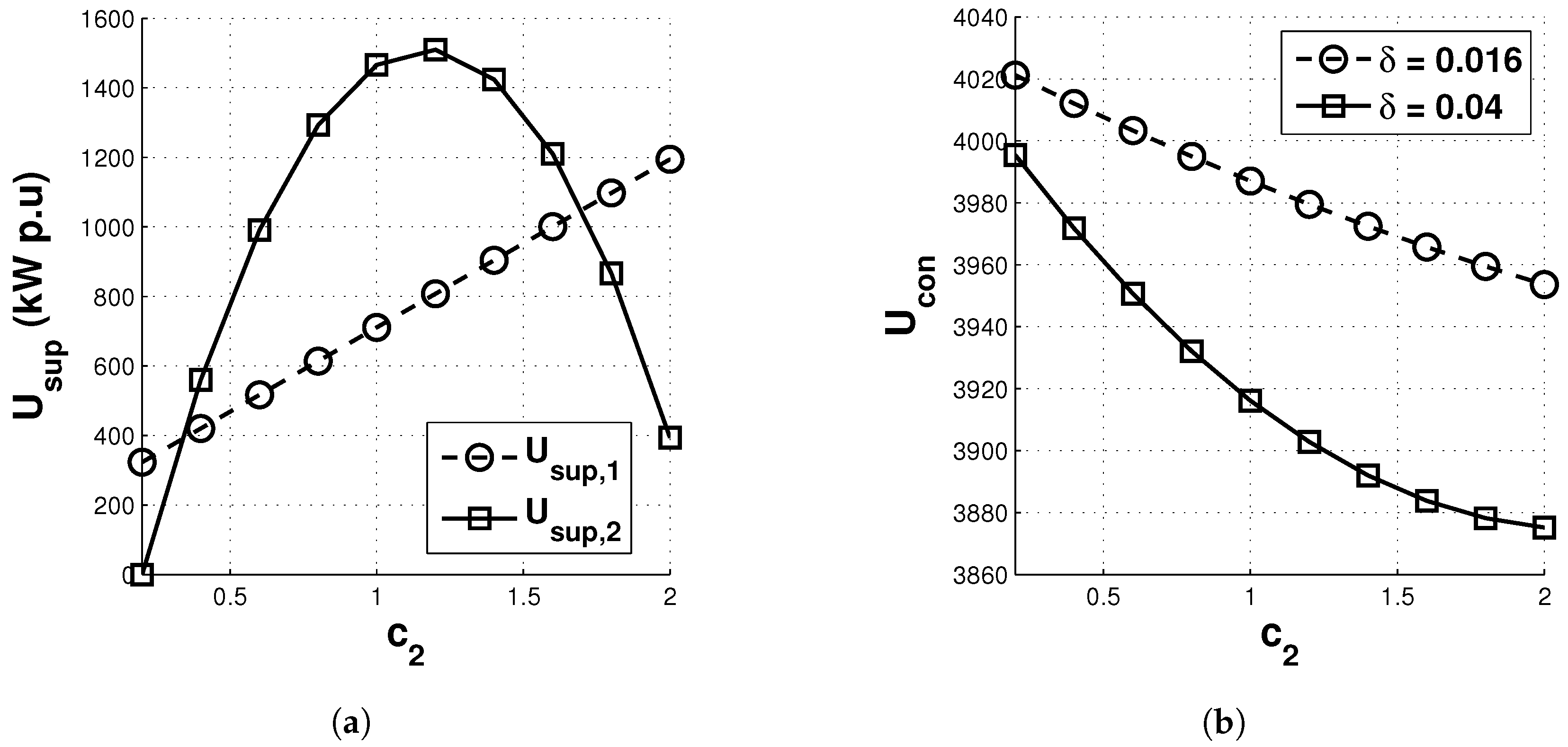
Based on the results of Figure 2, we analyze the utility of the supplier and the net utility of consumers as the price offered by supplier 2 varies. Figure 3b shows that the utility of supplier 2 is concave in price (from proposition 4), and the utility of supplier 1 increases with price . For each price offered by supplier 2, supplier 1 offers a price based on the best-response strategy to maximize its own utility. Therefore, until = 1.2, supplier 2 will increase the utility with ; however, it decreases with over 1.2. Thus, supplier 1 will end up obtaining a higher utility than supplier 1. This is due to the amount of decrease in demand distribution to supplier 2 as the prices they offer increase. Conversely, the demand distribution to supplier 1 correspondingly increases, as shown in Figure 2. In addition, the increased price of supplier 2 affects the best strategy of the other suppliers (i.e., the optimal price of supplier 1 also increases). Thus, the net utility for consumers decreases with price , as shown in Figure 3b. In addition, as the value of increases, the net utility for the consumers gives more weight to the impact of price. Hence, the lower net utility for consumers is achieved due to the larger impact of price.
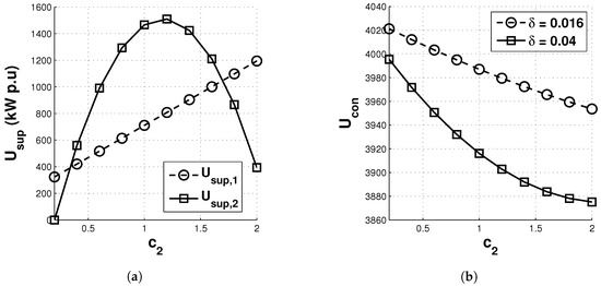
Figure 3.
(a) Utility of supplier and (b) net utility of consumers ( = 0.016, 0.04) as the price offered by supplier 2 varies.
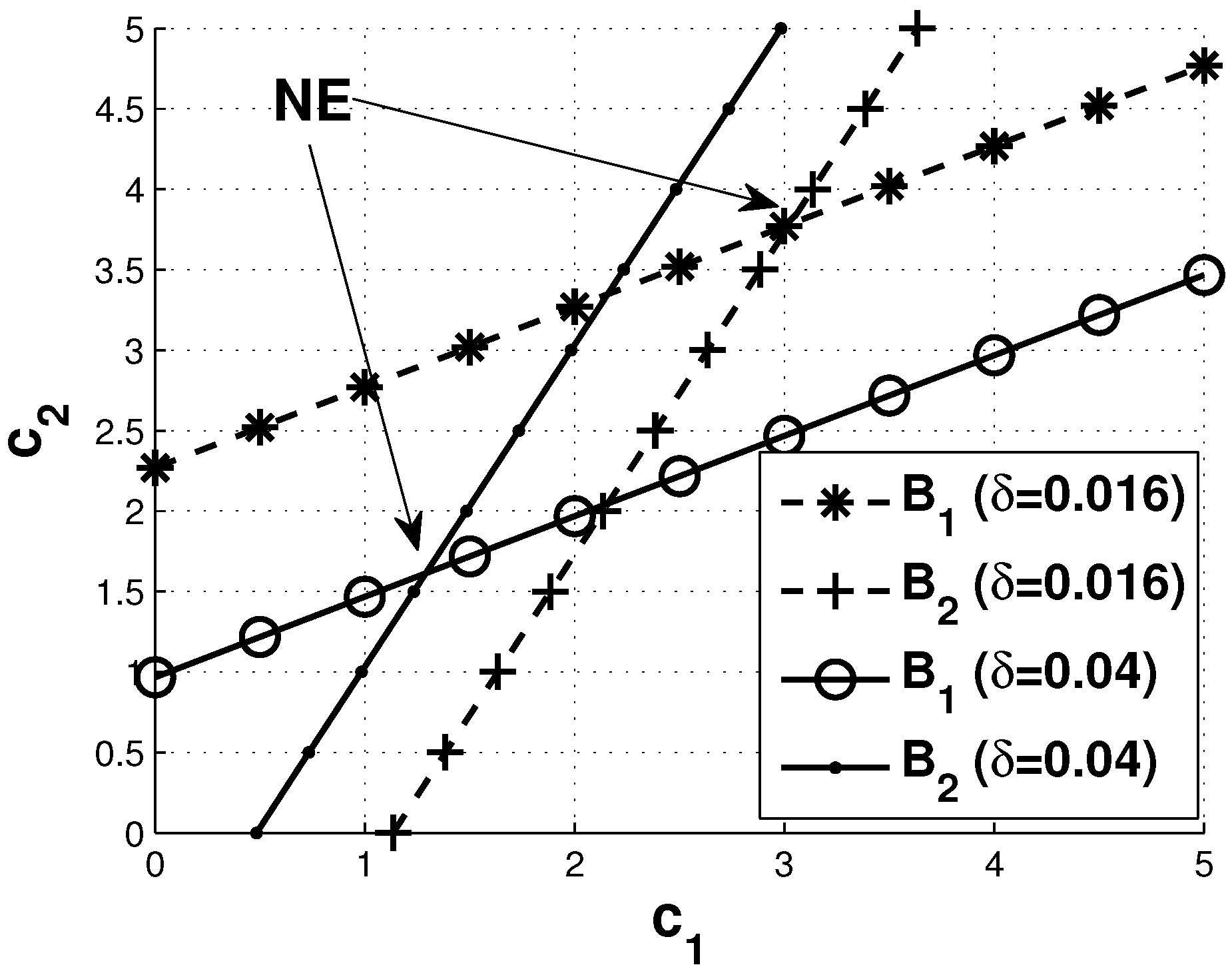
Figure 4 shows the best response functions and NE of the non-cooperative competitive pricing for the two suppliers. This is derived from Algorithm 2. This figure graphically shows the existence and uniqueness of the NE. As shown, there is only one point of intersection, which is the NE of prices offered to consumers by suppliers. In this case, as the value of increases, the NE provides less value due to the greater impact of price on consumers.
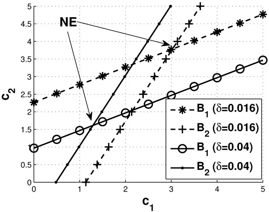
Figure 4.
Existence and uniqueness of the Nash equilibrium (NE) in the non-cooperative competitive pricing game among suppliers.
5.3. Utility of Suppliers and Net Utility of Consumers According to the Number of Suppliers
We investigate the effect of the number of suppliers on the net utility of consumers and the utility of suppliers and the optimal price. Here, we assume that the specification of different suppliers is identical to that of supplier 1. As shown in Figure 5a, the optimal price decreases with an increase in the number of suppliers. As the number of suppliers increases, the competition among them becomes more severe, and thus the average price decreases. Therefore, the utility for the supplier decreases due to the reduced optimal price, as shown in Figure 5. Conversely, Figure 5c shows that the net utility for consumers increases as the number of suppliers increases. Moreover, with the increase in the value of (from = 0.016 to = 0.04), the optimal price for suppliers decreases because the price now has a greater impact on the net utility of consumers than power loss penalty, as shown in Figure 5a. This means that the utility of the suppliers also decreases, as shown in Figure 5.
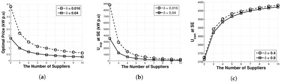
Figure 5.
(a) Optimal price, (b) utility of the supplier, and (c) net utility of consumers at the Stackelberg equilibrium (SE) as the number of suppliers varies.
6. Conclusions and Future Works
We analyzed and evaluated a demand-side management problem in which multiple suppliers with heterogeneous energy sources compete with each other by setting the unit price of each energy source. Then, consumers cooperatively react to the suppliers’ decisions on prices by deciding how to request their aggregated demand from multiple suppliers. To do this, we first modeled the utility functions for consumers and suppliers, respectively. For suppliers, the utility function was designed considering the revenue acquired from consumers and the cost of electric power generation. For consumers, the net utility function considers the consumers’ satisfaction, the price to pay, and the power loss during transmission. In considering the interactions between consumers and suppliers, the problem was formulated as a Stackelberg game. Based on the numerical results, we represented the relationship between price and demand, which affects both the game and the suppliers’ strategy. Finally, we showed that the proposed scheme converges well to an equilibrium point. Future work stemming from this study should accommodate dynamic game models with time varying analysis from a practical perspective.
Acknowledgments
This work was supported in part by the MSIT (Ministry of Science and ICT), Korea, under the National Program for Excellence in Software supervised by the IITP (Institute for Information & Communications Technology Promotion) (2015-0-00932) and BK 21 plus program.
Author Contributions
Joohyung Lee wrote the paper, designed ideas and performed the modelling as a corresponding author; Kireem Han performed the evaluations and analyzed the data. During the manuscript preparation Junkyun Choi helped to improve the paper content’s quality.
Conflicts of Interest
The authors declare no conflicts of interest.
Appendix A
This appendix provides the mathematical proof of the theorem represented in Section 4.
Proof of Theorem 2.
(1) Positivity.
Because > 0, > 0, and > 0, the first and second items in the best response function (26) are always greater than 0. In addition, is also positive due to this assumption. Because the best response function is a sum of positive terms, we can obtain the positivity of the best response function:
(2) Monotonicity.
Here, the problem for showing monotonicity can be reduced to providing . Taking the derivative of the best response function with respect to for , we obtain
In addition, taking the derivative of the best response function with respect to for and , we obtain
(3) Scalability.
Based on Eqaution (26) for all , we obtain
which satisfies scalability. ☐
References
- Arnold, G.W. Challenges and Opportunities in Smart Grid: A Position Article. Proc. IEEE 2011, 99, 922–927. [Google Scholar] [CrossRef]
- Saad, W.; Han, Z.; Poor, H.V.; Basar, T. Game-Theoretic Methods for the Smart Grid: An Overview of Microgrid Systems, Demand-Side Management, and Smart Grid Communications. IEEE Signal Process. Mag. 2012, 29, 86–105. [Google Scholar]
- Maharjan, S.; Zhu, Q.; Zhang, Y.; Gjessing, S.; Basar, T. Demand Response Management in the Smart Grid in a Large Population Regime. IEEE Trans. Smart Grid 2016, 7, 189–199. [Google Scholar] [CrossRef]
- Lee, J.; Guo, J.; Choi, J.; Zukerman, M. Distributed Energy Trading in Microgrids: A Game-Theoretic Model and Its Equilibrium Analysis. IEEE Trans. Ind. Electron. 2015, 62, 3524–3533. [Google Scholar] [CrossRef]
- Park, S.; Lee, J.; Bae, S.; Hwang, G.; Choi, J. Contribution-Based Energy-Trading Mechanism in Microgrids for Future Smart Grid: A Game Theoretic Approach. IEEE Trans. Ind. Electron. 2016, 63, 4255–4265. [Google Scholar] [CrossRef]
- Jeon, J.H.; Lee, J.; Choi, J.K. A Distributed Power Allocation Scheme for Base Stations Powered by Retailers with Heterogeneous Renewable Energy Sources. ETRI J. 2016, 38, 746–756. [Google Scholar] [CrossRef]
- Su, C.L.; Kirschen, D. Quantifying the Effect of Demand Response on Electricity Markets. IEEE Trans. Power Syst. 2009, 24, 1199–1207. [Google Scholar]
- Ibars, C.; Navarro, M.; Giupponi, L. Distributed Demand Management in Smart Grid with a Congestion Game. In Proceedings of the IEEE Smart Grid Communications, Gaitherburg, MD, USA, 4–6 October 2010; pp. 495–500. [Google Scholar]
- Mohsenian-Rad, A.; Wong, V.W.S.; Jatskevich, J.; Schober, R.; Leon-Garcia, A. Autonomous Demand-Side Management Based on Game-Theoretic Energy Consumption Scheduling for the Future Smart Grid. IEEE Trans. Smart Grid 2010, 1, 320–331. [Google Scholar] [CrossRef]
- Logenthiran, T.; Srinivasan, D.; Shun, T.Z. Demand Side Management in Smart Grid Using Heuristic Optimization. IEEE Trans. Smart Grid 2011, 3, 1244–1252. [Google Scholar] [CrossRef]
- Guan, X.; Ho, Y.C.; Pepyne, D.L. Gaming and Price Spikes in Electric Power Markets. IEEE Trans. Power Syst. 2001, 16, 402–408. [Google Scholar] [CrossRef]
- Soliman, H.M.; Leon-Garcia, A. Game-theoretic demand-side management with storage devices for the future smart grid. IEEE Trans. Smart Grid 2014, 5, 1475–1485. [Google Scholar] [CrossRef]
- Yu, M.; Hong, S.H. A real-time demand-response algorithm for smart grids: A stackelberg game approach. IEEE Trans. Smart Grid 2016, 7, 879–888. [Google Scholar] [CrossRef]
- Zhang, D.; Li, S.; Sun, M.; O’Neill, Z. An optimal and learning-based demand response and home energy management system. IEEE Trans. Smart Grid 2016, 7, 1790–1801. [Google Scholar] [CrossRef]
- AlSkaif, T.; Zapata, M.G.; Bellalta, B.; Nilsson, A. A distributed power sharing framework among households in microgrids: A repeated game approach. Computing 2017, 99, 23–37. [Google Scholar] [CrossRef]
- Li, C.; Tang, S.; Cao, Y.; Xu, Y.; Li, Y.; Li, J.; Zhang, R. A New Stepwise Power Tariff Model and Its Application for Residential Consumers in Regulated Electricity Markets. IEEE Trans. Power Syst. 2013, 28, 300–308. [Google Scholar] [CrossRef]
- Liu, Y.; Guan, X. Purchase Allocation and Demand Bidding in Electric Power Markets. IEEE Trans. Power Syst. 2003, 18, 106–112. [Google Scholar]
- Ma, J.; Deng, J.; Song, L.; Han, Z. Incentive mechanism for demand side management in smart grid using auction. IEEE Trans. Smart Grid 2014, 5, 1379–1388. [Google Scholar] [CrossRef]
- Samadi, P.; Mohsenian-Rad, H.; Schober, R.; Wong, V.W.S. Advanced Demand Side Management for the Future Smart Grid Using Mechanism Design. IEEE Trans. Smart Grid 2012, 3, 1170–1180. [Google Scholar] [CrossRef]
- Shengrong, B.; Yu, F.R.; Liu, P. Dynamic pricing for demand-side management in the smart grid. In Proceedings of the IEEE Online Conference on Green Communication, New York, NY, USA, 26–29 September 2011; pp. 47–51. [Google Scholar]
- Yang, P.; Tang, G.; Nehorai, A. A Game-Theoretic Approach for Optimal Time-of-Use Electricity Pricing. IEEE Trans. Power Syst. 2013, 28, 884–892. [Google Scholar] [CrossRef]
- Li, C.; Yu, X.; Yu, W.; Chen, G.; Wang, J. Efficient Computation for Sparse Load Shifting in Demand Side Management. IEEE Trans. Smart Grid 2017, 8, 250–261. [Google Scholar] [CrossRef]
- Marzband, M.; Javadi, M.; Domínguez-García, J.L.; Moghaddam, M.M. Non-cooperative game theory based energy management systems for energy district in the retail market considering DER uncertainties. IET Gener. Transm. Distrib. 2016, 10, 2999–3009. [Google Scholar] [CrossRef]
- Song, L.; Xiao, Y.; Van Der Schaar, M. Demand side management in smart grids using a repeated game framework. IEEE J. Sel. Areas Commun. 2014, 32, 1412–1424. [Google Scholar] [CrossRef]
- Stephens, E.R.; Smith, D.B.; Mahanti, A. Game theoretic model predictive control for distributed energy demand-side management. IEEE Trans. Smart Grid 2015, 6, 1394–1402. [Google Scholar] [CrossRef]
- Yu, M.; Hong, S.H. Incentive-based demand response considering hierarchical electricity market: A Stackelberg game approach. Appl. Energy 2017, 203, 267–279. [Google Scholar] [CrossRef]
- Maharjan, S.; Zhu, Q.; Zhang, Y.; Gjessing, S.; Basar, T. Dependable demand response management in the smart grid: A Stackelberg game approach. IEEE Trans. Smart Grid 2013, 4, 120–132. [Google Scholar] [CrossRef]
- Alshehri, K.M.A. Multi-Period Demand Response Management in the Smart Grid: A Stackelberg Game Approach. Ph.D. Thesis, University of Illinois at Urbana-Champaign, Champaign, IL, USA, 2015. [Google Scholar]
- Saad, W.; Han, Z.; Poor, H.V. Coalitional Game Theory for Cooperative Micro-Grid Distribution Networks. In Proceedings of the Communications Workshops (ICC) ’11, Kyoto, Japan, 5–9 June 2011. [Google Scholar]
- Callahan, J.J. Advanced Calculus: A Geometric View; Springer Science & Business Media: New York, NY, USA, 2010. [Google Scholar]
- Palomar, D.P.; Chiang, M. A tutorial on decomposition methods for network utility maximization. IEEE J. Sel. Areas Commun. 2006, 24, 1439–1451. [Google Scholar] [CrossRef]
- Boyd, S.; Vandenberghe, L. Convex Optimization; Cambridge University Press: Cambridge, UK, 2004. [Google Scholar]
- Bertsekas, D.P. Non-Linear Programming; Athena Scientific: Beimont, MA, USA, 2003. [Google Scholar]
- Dos Santos Gromicho, J. Quasiconvex Optimization and Location Theory (Applied Optimization); Springer: New York, NY, USA, 1998. [Google Scholar]
- Mas-Colell, A.; Whinston, M.D.; Green, J.R. Microeconemic Theory; Oxford University: Oxford, UK, 1995. [Google Scholar]
- Machowski, J.; Bialek, J.W.; Bumby, J.R. Power Systems Dynamics: Stability and Control; Wile: New York, NY, USA, 2008. [Google Scholar]


© 2017 by the authors. Licensee MDPI, Basel, Switzerland. This article is an open access article distributed under the terms and conditions of the Creative Commons Attribution (CC BY) license (http://creativecommons.org/licenses/by/4.0/).