Article

Performance Analysis of Conjugate Gradient Algorithms Applied to the Neuro-Fuzzy Feedback Linearization-Based Adaptive Control Paradigm for Multiple HVDC Links in AC/DC Power System

Department of Electrical Engineering, COMSATS Institute of information Technology, 22060 Abbottabad, Pakistan
*
Author to whom correspondence should be addressed.
Energies 2017, 10(6), 819; https://doi.org/10.3390/en10060819
Submission received: 23 March 2017 / Revised: 24 May 2017 / Accepted: 5 June 2017 / Published: 16 June 2017
(This article belongs to the Section F: Electrical Engineering)

Abstract

:
The existing literature predominantly concentrates on the utilization of the gradient descent algorithm for control systems’ design in power systems for stability enhancement. In this paper, various flavors of the Conjugate Gradient (CG) algorithm have been employed to design the online neuro-fuzzy linearization-based adaptive control strategy for Line Commutated Converters’ (LCC) High Voltage Direct Current (HVDC) links embedded in a multi-machine test power system. The conjugate gradient algorithms are evaluated based on the damping of electro-mechanical oscillatory modes using MATLAB/Simulink. The results validate that all of the conjugate gradient algorithms have outperformed the gradient descent optimization scheme and other conventional and non-conventional control schemes.

1. Introduction

In recent years, the rapid growth in energy consumption and the implementation of the deregulated environment have resulted in the highly interconnected and stressed infrastructure of the power system. A change in the operating condition at any one location can have a magnified impact over a wide area as it propagates through the electrical network. Under the stressed operating conditions, even a small disturbance can threaten the stability of the power system and generate power system oscillations. Among these, Low-Frequency Oscillations (LFOs) would limit the power transfer capabilities between different interconnected areas and have a great impact on the most secure and economical operation of the power systems [1].
Rapid and effective damping of LFOs is an important issue as the sustained LFOs may result in almost instantaneous large-scale cascading failures. To avoid the economic loss and daily life interruption, it is highly necessary to dampen LFOs to continue the secure operation of the power system [2,3]. To improve the stability of the power system, a solution might be to utilize controllable power components within the system. One such component is the HVDC link [4].
Over the last few decades, rapid growth has been observed in the application of the HVDC technology in electric power transmission systems due to its economical and technical advantages. Mainly, HVDC transmission systems are employed to transmit electric bulk power over long distances and interconnect asynchronous AC systems having different frequencies [5]. Available technology options for HVDC transmission system includes Line Commuted Converters (LCC) and forced commutated converters. The LCC-HVDC systems have evolved as a much more mature and reliable technology [6]. The simply structured classic LCC-HVDC systems are available in high power ratings with lower power losses [7]. As HVDC system operation involves no inertia, it is possible to rapidly control the power flow through the HVDC link. The instant variation in power flow can be used to improve system operating flexibility, as well as maintain the stability of the power system during perturbed operating conditions. The provision of appropriate supplementary damping control of the classical HVDC system provides modulation of power flow through the HVDC link and effectively mitigates inter-area oscillations of interconnected power systems [8]. Recently, extensive research has been carried out to propose Power Oscillation Damping (POD) controllers applying classical control theory, optimal control schemes, robust control methods and the feedback linearization technique [9,10,11,12,13,14,15,16]. Classical control theory-based POD controllers are designed with a first-order approximation of the system dynamics at a certain operating condition. This method provides adequate damping for a system operating in the vicinity of equilibrium. However, their performance may decline due to the wide-ranging and rapidly varying operating conditions of the highly nonlinear and stochastic nature of the power system [17]. The linear optimal control schemes are based on the system model, which is linearized at a specific operating point and suffers the same drawbacks and limitations as classical control [18]. Robust control improves the performance of classical POD control. However, it requires an upper bound on uncertainties and is deficient in learning. Its performance deteriorates in a highly nonlinear power system with increased uncertainties [19].
For highly nonlinear systems, differential geometry-based Feedback Linearization Control (FBLC) is a better option to model a nonlinear control scheme [20]. However, it requires having exact knowledge of the system nonlinearities. Model uncertainty can result in degraded performance and hence limited applications in the power system [21]. The POD controller realization based on an adaptive feedback linearization becomes more suitable for applications in the highly nonlinear power systems with unknown or uncertain parameters [22]. Although model-based methods for identification and control of plants dynamics are well established and widely used, they may not provide satisfactory performance in today’s power system. Artificial intelligence-based control techniques have been applied for systems with both un-modeled dynamics and uncertainty in the parameter [23].
In [24], Artificial Neural Network (ANN)-based FBLC is employed to improve power system stability by mitigating LFOs. The opaque nature of ANNs includes learning capability, and they are capable of parallel processing. ANNs entail an ample amount of problem data for their training and are prone to overfitting [25]. ANNs’ drawbacks are tackled by the integration of their merits and the Fuzzy Logic System (FLS) that results in a more intelligent Adaptive Neuro-Fuzzy Inference System (ANFIS). The combination of FLS and ANNs acquires the capabilities of robustness, parallel processing and learning capability from ANNs and the imprecise knowledge-based modeling capability of the simple and natural structure FLS. ANFIS is dynamic and capable of learning from experience with sample data to estimate a function without any mathematical model. The online optimization of the parameters of ANFIS enhances its fast and accurate learning capabilities to achieve the desired output [26,27].
The gradient-based back-propagation algorithm has been widely used as a learning algorithm for ANFIS [28]. The Steepest Descent (SD) algorithm follows the negative of the gradient to approach the desired local minimum in a zigzag path. Newton methods have faster convergence than the SD method, but require computation of the Hessian and its inverse. A prominent iterative Conjugate Gradient (CG) method computes new search directions by using only one previous search vector at each time step and does not follow a pre-specified direction of the negative of the gradient. The speed of convergence is better than the SD method as the CG algorithm moves in the non-interfering directions. Computation of the Hessian is not a prerequisite in CG algorithms. It requires less memory to operate and less computation as compared to Hessian-based methods [29]. With simple implementation and fast convergence, CG methods become numerically competitive for applications in a highly nonlinear power system [30,31]. Furthermore, a real-time adaptation of ANFIS parameters has a swift response in comparison with batch mode adaptation and rapidly optimizes the parameters of ANFIS [32]. The performance of FBLC is further improved through on-line tuning of its coefficients. Optimized coefficients keep the control magnitude bounded and effective over a wide range of operating conditions [33]. Simple implementation of the Least Mean Square (LMS) algorithm makes it the most prevalent adaptive algorithm. Anyhow, the LMS algorithm is sensitive to the scaling of its input and exhibits data-dependent slow convergence behavior. Its variant, normalized Least Mean Square (nLMS) algorithm, is as simple as LMS and more robust. The nLMS algorithm is more stable on average than LMS and shows an improved balance between simplicity and performance in real-time applications [34].
A MIMO Adaptive Neuro-Fuzzy Feedback Linearization Control (ANFFBLC) for multiple HVDC links has been proposed in [35]. The ANFIS architecture is employed for real-time identification of unknown nonlinear dynamics of the power system. ANFIS parameters are optimized through a nonlinear CG algorithm proposed by Hager and Zhang. FBLC coefficients are on-line tuned to track the power system output for an extensive operating conditions. On-line self-tuning of FBLC coefficients and real-time adaptive neuro-fuzzy identification aspects of ANFFBLC make it an appropriate POD control for HVDC systems. The main contributions of this research include:
  • Implementation of the SD algorithm and six CG methods for online optimization of ANFFBLC parameters.
  • Evaluation and comparison of damping performance of the SD algorithm and six CG methods along with conventional and non-conventional control schemes.
Different case studies are performed in a multi-area AC/DC test power system to validate the damping performance of ANFFBLC with different CG algorithms. Results show a promising response with ANFFBLC and improved stability of the power system as compared with conventional and non-conventional control schemes.
The rest of the paper is organized as follows. Section 2 describes the modeling and control of the AC/DC power system. The proposed closed-loop control system design is explained in Section 3. Results are presented and discussed in Section 4. Section 5 concludes the findings of this research work.

2. AC/DC Power System Model Description

The major components of test AC/DC power system comprise the synchronous generators with control, LCC-HVDC links, transmission lines and transformers. Synchronous machines and control dynamics are expressed by differential equations, while algebraic equations describe the load flow and network model.

2.1. Power System Components Modeling

The synchronous machines with their associated control constitutethe major components of the modern power system. This research work implements a sixth order synchronous machine, while considering the dynamics of the stator, field and damper windings. The sixth order model of the i-th synchronous machine is given by the following differential equations [36].
T d o d d t E q = E f d E q ( x d x d ) I d x d x d ( x d x l s ) 2 ( ψ 1 d + ( x d x l s ) I d E q )
T d o d d t ψ 1 d = ψ 1 d + E q + ( x d x l s ) I d
T q o d d t E d = E d + ( x q x q ) I q x q x q ( x q x l s ) 2 ( ψ 2 q + ( x q x l s ) I q + E d )
T q o d d t ψ 2 q = ψ 2 q E d + ( x q x l s ) I q
d d t δ = ω r ω s
d d t ω r = 1 2 H P m P e D Δ ω r
where:
  • E f d is the field voltage.
  • E d / q is the transient voltage in the d/q-axis.
  • I d / q is the armature current in the d/q-axis.
  • x d / q , x d / q , x d / q are synchronous, transient and sub-transient reactances in the d/q-axis, respectively.
  • x l s is the armature leakage reactance.
  • T d o / q o is the transient time constants of the d/q-axis.
  • T d o / q o is the sub-transient time constants of the d/q-axis.
  • ψ 1 d is the d-axis flux linkage of the damper winding.
  • ψ 2 q is the q-axis flux linkage of the damper winding.
  • H is the inertia constant.
  • P e is the generator electrical power.
  • P m is the generator mechanical power.
  • δ is the generator rotor angle.
  • ω r is the generator rotor speed.
The dynamics in the d-axis are narrated by Equations (1) and (2), while Equations (3) and (4) define the dynamics in the q-axis. The swing equation of the synchronous machine is represented by Equations (5) and (6). With negligible stator’s resistance, the stator voltage and machine’s real power are given as:
E d = x q x l s x q x l s E d x q x q x q x l s ψ 2 q + x q I q
E q = x d x l s x d x l s E q + x d x d x d x l s ψ 1 d + x d I d
E t = E d 2 + E q 2
P e = E d I d + E q I q
where E t is the generator terminal voltage. The complete generator model includes a detailed nonlinear hydraulic turbine with a governor system. The excitation system is implemented with the IEEE Type 1 voltage regulator combined with an exciter. The long transmission line is modeled with the distributed parameter, and distribution lines are modeled with lumped parameters and π -representation. All transmission lines, transformers and loads are combined to model the power system network, and the nodal equations describe the relationships between the system voltages and currents.

2.2. HVDC Dynamics

LCC-HVDC is comprised of the commutation transformer, thyristor bridges, the AC filter system to limit the harmonic content in the AC current, the DC smoothing reactor, the mono-polar DC transmission line and the control system.

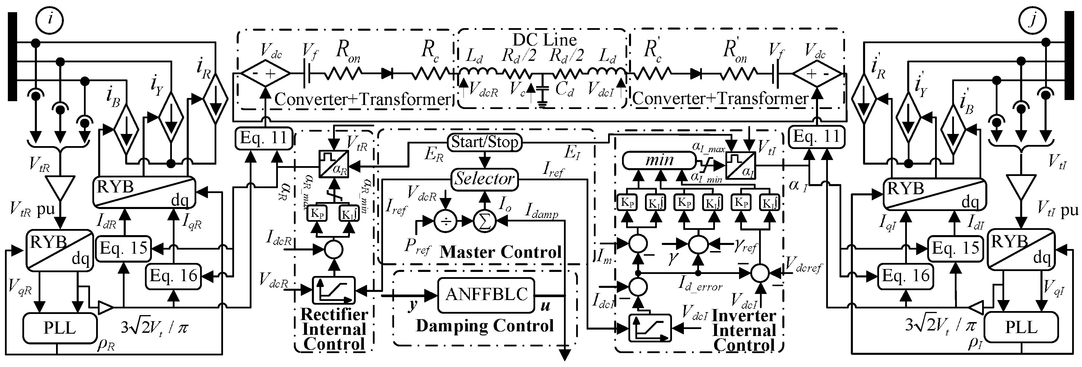
2.2.1. LCC-HVDC Converter Modeling

The LCC-HVDC system represented by an average model is shown in Figure 1. The variables are shown with appropriate subscripts I and R for the inverter and rectifier poles, respectively. The rectifier and inverter poles are average models of 12-pulse converters with equivalent DC voltage and AC current sources. The voltage source generates converter voltage at the DC side, and the current source injects the fundamental component of the current into the AC network. The linear model of the commutation transformer is also included in the average model representation. The model does not represent high-frequency switching harmonics, which are unnecessary for dynamic analysis and control dynamics. However, dynamics resulting from the control system and the power system interaction are preserved [37]. The rectifier and the inverter are interconnected through a DC transmission line with smoothing reactors for each pole.
The average DC voltage with firing delay angle, α is defined as:
V d c = 6 π π / 6 + α π / 6 + α 2 a V t cos ( ω t ) d ( ω t ) = 6 2 π a V t cos α
where V t is the converter AC bus voltage, a is the transformer’s off-nominal tap ratio and 6 2 π a V t = V d c o is the ideal no-load DC voltage; where:
6 2 π a V t = V d c o
The voltage source in the average model is powered by Equation (11). The figure also models the thyristor on-state voltage drop and losses in the converter and transformer. The diode represents the unidirectional current flow without any losses associated with it. The DC voltage at the rectifier and inverter, with the effect of commutation overlap, is given as:
V d c R = V d c o cos α 2 3 X c π I d c R
V d c I = V d c o cos γ 2 3 X c π I d c I
In the above equations, I d c is the converter direct current, X c is the commutation reactance and γ = π α μ is defined as the extinction advance angle. Here, μ is the commutation interval. The fundamental primary phase current injected into the AC line is computed in the d q -axis frame as:
I d = V d c o ( cos 2 α cos ( 2 α + 2 μ ) ) 4 6 a X c
I q = V d c o ( 2 μ + sin 2 α sin ( 2 α + 2 μ ) ) 4 6 a X c
μ = cos 1 cos α 2 X c I d V d c o α
The active and reactive power exchanged with the AC system is calculated as:
P a c = 2 π 6 a V d c o I d
Q a c = 2 π 6 a V d c o I q

2.2.2. DC Transmission System

The DC transmission system model includes a DC line with smoothing reactors at both pole terminals. The T-model for the DC line dynamics of the LCC-HVDC system is described by two reactor currents and a capacitor voltage. With DC voltages, V d c R and V d c I , available at the terminals of DC system, the dynamics of DC transmission line are given as [16]:
L d I d c R ˙ = V d c R V C I d c R R d 2
L d I d c I ˙ = V C V d I I d c I R d 2
C d V c ˙ = ( I d c R I d c I )
where R d , C d and V c are resistance, capacitance and voltage across the capacitance of the DC line, respectively.

2.2.3. LCC-HVDC Control

The control architecture of an LCC-HVDC system is implemented with internal control and external POD control. The rapid control of the desired power flow through HVDC link is realized through swift valve gate control. In the internal control, master control determines the appropriate current order I r e f and transmits the same to the rectifier and inverter controls. The current order is calculated as:
I r e f = P r e f V d c R + I d a m p
where P r e f is the desired HVDC power and the damping signal I d a m p is derived through ANFFBLC. During normal operation, the power order determines the current order, and I d a m p is zero. Under disturbed operating conditions, the ANFFBLC generates the appropriate damping signal that adjusts the I r e f and, hence, modulates HVDC power. The conventional Proportional-Integral (PI)-based pole control generates the respective ignition delay angle α subject to current reference and the Voltage-Dependent Current Order Limiter (VDCOL). In the case of low commutating voltage, the VDCOL redefines the reduced current reference according to reduced DC voltage once it becomes less than the predefined threshold [38].
In the normal operation, the rectifier maintains a constant current through the DC transmission system. The control mode is shifted to constant ignition angle with minimum delay angle α m i n during disturbed operating conditions. The rectifier current control is defined as:
α ˙ R = K P I ˙ d c R + K I I e R
where the current error is I e R = I d c R I r e f and α R _ m i n α R α R _ m a x . The inverter is operated in a constant extinction angle control mode that maintains the DC system voltage at the inverter. For the reduced commutation voltage in distressed operating conditions, the inverter control switches to constant current control mode. The dynamics of the inverter current control, voltage control and gamma control are described respectively as:
α ˙ I I = K P I ˙ d c I + K I I e I
α ˙ I V = K P V ˙ d c I + K I V e I
α ˙ I γ = K P γ ˙ + K I γ e I
α I | α I _ m i n α I _ m a x = min { α I I , α I V , α I γ }
where current, voltage and γ error, respectively, are I e I = I d c I I r e f + I m , V e I = V d c I V d c r e f V d c m I r e f I d c I I m , γ e I = γ γ r e f γ m I r e f I d c I I m . The inverter control also provides current support for the situation when the DC current drops below a threshold equal to I r e f I m . Furthermore, α for the inverter is maintained to ensure γ γ m i n [39]. I m , V m and γ m are current, voltage and extinction advance angle margins at the inverter pole, respectively.

3. Closed-Loop Control System Design

The proposed ANFFBLC scheme is a model-free indirect control strategy and requires minimal knowledge of the power system. As shown in Figure 2, the dynamics of the AC/DC power system are identified through an Adaptive Neuro-Fuzzy Identifier (ANFI) using the Wide-Area Measurement System (WAMS)-based measured speed signals of generators. The CG algorithm on-line optimizes the ANFI parameters to minimize the identification error. The coefficients of the FBLC are also tuned through the nLMS algorithm to maintain its performance over a wide range of operating conditions. Based on the identified power system model, the ANFFBLC generates the appropriate damping signal for each HVDC link. The following section explains the implementation and function of the ANFFBLC to improve the damping of the power system oscillations.

3.1. Feedback Linearization Control

Feedback linearization is a well-known technique used to transform a nonlinear system into a linear one by a state transformation and nonlinear feedback. A well developed linear control design now can be applied to a linearized system [40]. Consider an-th-order multi-variable nonlinear system [41]:
y 1 n = f 1 ( x ) + g 11 ( x ) u 1 + + g 1 m ( x ) u m y m n = f m ( x ) + g m 1 ( x ) u 1 + + g m m ( x ) u m
where x = [ x 1 , , x 1 n 1 , , x m , x 1 n 1 ] T m n is the state variable available for measurement, u = [ u 1 , u 2 , , u m ] T m represents the control input and y = [ y 1 , y 2 , , y m ] T m is the output of MIMO nonlinear system. f τ ( x ) m and g τ h ( x ) m × m represent unknown smooth nonlinearities of the dynamic system with τ , h = 1 , 2 , , m . The system in Equation (29) can also be expressed in companion form as:
y = f ( x ) + G ( x ) u
where y n = y 1 n , y 2 n , , y m n T m , f ( x ) = f 1 ( x ) , f 2 ( x ) , , f m ( x ) T m and G ( x ) = g 11 g 1 m g m 1 g m m m × m .
The control objective is to derive control law u = [ u 1 , u 2 , , u m ] T that forces the output y ( t ) = [ y 1 ( t ) , y 2 ( t ) , , y m ( t ) ] T to follow the a desired trajectory y d ( t ) = [ y 1 d ( t ) , y 2 d ( t ) , , y m d ( t ) ] T . The error matrix e ̲ is defined as:
e ̲ = y 1 y 1 d y 2 y 2 d y m y m d y ˙ 1 y ˙ 1 d y ˙ 2 y ˙ 2 d y ˙ m y ˙ m d y 1 ( n 1 ) y 1 d ( n 1 ) y 2 ( n 1 ) y 2 d ( n 1 ) y m ( n 1 ) y m d ( n 1 )
The filter tracking error Υ is defined as:
Υ T = θ 1 θ 2 θ n 1 1 T e ̲ = Θ T 1 e ̲
where Θ = θ 1 θ 2 θ n 1 is a vector of FBLC coefficients, and its appropriate choice ensures that z n 1 + θ n 1 z n 1 + + θ 1 is asymptotically stable, i.e., e ̲ ( k ) 0 as Υ ( k ) 0 . The constant value of Θ does not provide desired performance over a wide range of operating conditions. In this research work, Θ is updated at each time step using the nLMS-based self-tuning scheme. The derivative of Equation (32) results in:
Υ ˙ T = θ 1 θ 2 θ n 1 1 T y ˙ 1 y ˙ 1 d y ˙ 2 y ˙ 2 d y ˙ m y ˙ m d y ¨ 1 y ¨ 1 d y ¨ 2 y ¨ 2 d y ¨ m y ¨ m d y 1 n y 1 d n y 2 n y 2 d n y m n y m d n
Υ ˙ T = y 1 n y 2 n y m n T + y 1 d n y 2 d n y m d n T + 0 Θ T e ̲ = y 1 n y 2 n y m n + y D T 1 × m
Using Equations (30) and (34), we have:
Υ ˙ = y n + Y D = f ( x ) + G ( x ) u + y D
Using Υ = exp ( K Γ t ) Υ ˙ = K Γ Υ and K Γ > 0 ensures that e ̲ 0 as Υ 0 . Therefore, the above equation can be written as:
K Γ Υ = f ( x ) + G ( x ) u + y D
For the known nonlinear functions f ( x ) and G ( x ) , the following control law is designed according to the feedback linearization method, which would cancel the nonlinearities of the system and would bring Υ to zero:
u = G 1 ( x ) [ f ( x ) K Γ Υ y D ]
However, it is impractical to implement the control law if the nonlinear functions f and G are uncertain or unknown. Therefore, this study proposes to identify the nonlinear functions f ^ and G ^ at each time-step through an Adaptive Neuro-Fuzzy Identifier (ANFI) and to online optimize the design parameter Θ . The control law is now given as:
u = G ^ 1 ( x ) [ f ^ ( x ) Γ ]
where Γ = K Γ Υ y D .
Assumption 1.
As the nonlinear MIMO system is controllable, G ( x ) m × m is invertible for all x U c m n .
The following section explains the identification of nonlinear functions and online estimation of the design parameter.

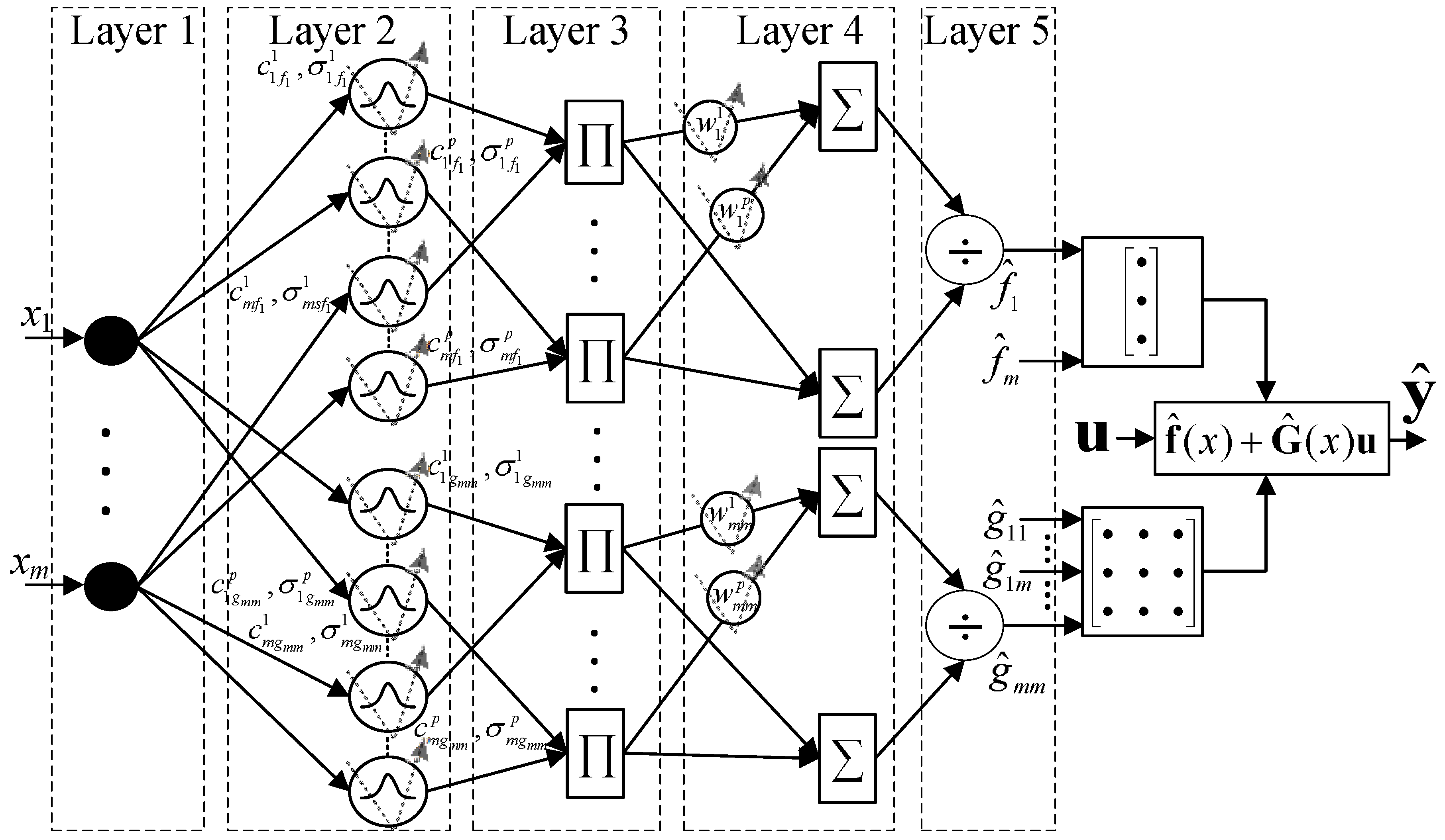
3.2. Adaptive Neuro-Fuzzy Identification

The five-layered ANFI architecture was implemented to identify the nonlinear dynamics of the power system. The inputs to the ANFI are relative speed deviations of different machines w.r.t. the swing machine, and the outputs are the identified nonlinear dynamics of the power system. In the forward pass, the whole network works in a layer fashion, and in the backward pass, error signals are propagated to update the antecedent and consequent parts’ parameters according to the chain rule.
Assumption 2.
The system relative degree n is known, and y, y ˙ ,, y n are bounded output and available for measurement.
The ANFI architecture of Figure 3 is implemented with m 2 + m neuro-fuzzy subsystem blocks that realizes a fuzzy IF-THEN rule in the following form:
  • Rule j f : If x 1 is F τ 1 j and x 2 is F τ 2 j and ⋯ and x m is F τ m j , Then f τ ^ is w f τ j
  • Rule j g : If x 1 is G τ h 1 j and x 2 is G τ h 2 j and ⋯ and x m is G τ k m j , Then g τ h ^ is w g τ h j
where F τ i j and G τ h i j represent fuzzy sets of the antecedent part for the i-th input, i = 1 , 2 , , m , and the j-th rule, j = 1 , 2 , , p , and w f τ j and w g τ h j , τ , h = 1 , 2 , , m , are the consequent weights. The network is implemented with Gaussian membership functions in the antecedent part, a product inference engine and singleton variables in the consequent part.
The function of the nodes in each layer is defined as:
Layer 1: Each node in this layer only transmits input values to the next layer.
Layer 2: The adaptive nodes represent the input fuzzy sets described by the Gaussian membership function. The output of each node is calculated as:
A i j = exp 1 2 x i c i j σ i j 2
where c i j and σ i j , receptively, are the mean and standard deviation of the Gaussian membership function for the j-th term of the i-th input variable x i .
Layer 3: Rule nodes constitute the antecedent of the fuzzy rule base. The firing strength of each rule is calculated using the product T-norm. The output of this layer for the j-th rule is defined as:
A j = i = 1 n A i j ( x i )
Layer 4: Nodes in Layer 4 are called consequent nodes and represent the possible THEN-part of the fuzzy rules. The weights of the adaptive links in this layer represent the singleton w f τ j and w g τ h j . The nodes in this layer compute the weighted firing strengths of each rule from the previous layer.
Layer 5: Nodes in this layer calculate the normalized sum of weighted firing strengths over the sum of firing strengths. The computed defuzzified crisp outputs are identified f ^ τ ( x ) and g ^ τ h ( x ) and given as:
f ^ τ = j = 1 p w f τ j A j j = 1 p A j = j = 1 p ξ j w f τ j
g ^ τ h = j = 1 p w g τ h j A j j = 1 p A j = j = 1 p ξ j w g τ h j
where ξ j = A j j = 1 p A j is the j-th fuzzy basis function. The MIMO nonlinear system is identified as:
y ^ = f ^ ( x ) + G ^ ( x ) u
where f ^ ( x ) = f ^ 1 ( x ) f ^ 2 ( x ) f ^ m ( x ) T and G ^ ( x ) = g ^ 11 ( x ) g ^ 1 m ( x ) g ^ m 1 ( x ) g ^ m m ( x ) .
The identification error, e I , is defined as the error between identified and real dynamics and given as:
e I ( k ) = 1 2 ε T ε = 1 2 y ^ ( k ) y ( k ) 2
The objective is to accurately identify the dynamics of the power system by minimizing the identification error e I ( k ) . The conjugate gradient-based parameter learning algorithm is developed to minimize the error through optimization of the parameters of the membership functions and the link weights in the consequent part. The following section explains the CG-based optimization algorithm for the adaptive parameters of ANFI.

Conjugate Gradient Algorithm for Parameter Optimization

CG algorithms comprise a class of optimization algorithms that have strong local and global convergence properties. The nonlinear CG methods are relatively robust in numerical computation and provide sufficient descent independence of line search [42]. Our problem is to minimize the identification error by adapting the parameters of the ANFFBLC.
ρ = { c i f τ j , σ i f τ j , c i g τ h j , σ i g τ h j , w f τ j , w g τ h j }
where ρ represents the adaptation parameters of the ANFIS. A nonlinear CG algorithm computes a sequence ρ k , k 1 with initial guess ρ 0 , using the recurrence as:
ρ ( k + 1 ) = ρ ( k ) + χ i d ( k )
where the χ > 0 is a design parameter and d ( k ) is the conjugate search direction, computed as:
d ( k ) = g ( k ) , k = 0 g ( k ) + β k d ( k 1 ) , k 1
Here, g ( k ) = e I ( ρ ) is the gradient of the error function at the k-th instant, and β k is the CG coefficient, chosen in such a way that the new search direction is orthogonal to the subspace generated by previous search directions. In this research work, the following different CG algorithms are opted to corresponding different choices for the computation of β k .
  • Fletcher and Reeves (FR) presented the first nonlinear CG algorithm with update choice for the CG coefficient, β k F R , given as [43]:
    β k F R = g ( k + 1 ) 2 g ( k ) 2
  • Polak-Ribière and Polayk (PRP) proposed a CG method that updated the CG coefficient, β k P R P , using the following formula [44].
    β k P R P = g ( k + 1 ) T g ( k + 1 ) g ( k ) [ g ( k ) ] T g ( k )
  • The CG algorithm suggested by Fletcher (CD) has a strong convergence property, and the coefficient, β k C D , is updated using [45]:
    β k C D = g ( k + 1 ) 2 d ( k ) T g ( k )
  • The effect of inexact linear search was considered by Liu and Storey (LS) to develop a generalized CG scheme with coefficient β k L S updated as [46]:
    β k L S = g ( k + 1 ) T g ( k + 1 ) g ( k ) d ( k ) T g ( k )
  • In [47], a CG algorithm was presented by Dai and Yuan (DY) with a sufficient descent property. The CG coefficient, β k D Y , is updated as:
    β k D Y = g ( k + 1 ) 2 d ( k ) T g ( k + 1 ) g ( k )
  • A modified CG algorithm is proposed by Hager and Zhang (HZ) that has a more complicated update formula [48]. The CG coefficient, β k N , is updated as:
    β k N = ( g ( k + 1 ) g ( k ) ) 2 d ( k ) g ( k + 1 ) g ( k ) 2 d ( k ) T g ( k + 1 ) g ( k ) T g ( k + 1 ) d ( k ) T g ( k + 1 ) g ( k )
All of these methods do not require the computation of the Hessian matrix that is usually preferred over the methods requiring the Hessian in each iteration. The gradient of identification error is computed in each iteration of the CG algorithm. Using the chain rule of differentiation, the gradient of Equation (44) w.r.t. the respective consequent part parameter is given as:
e I w f τ j = e I y ^ y ^ f ^ f ^ τ w f τ j = ε ξ f τ j
e I w g τ h j = e I y ^ y ^ g ^ τ h g ^ τ h w g τ h j = ε ξ g τ h j u
where e I y ^ = ε , y ^ f ^ τ = 1 , y ^ g ^ τ h = u , f ^ τ w f τ j = ξ f τ j and g ^ τ h w g τ h j = ξ g τ h j . For the identification of f ^ τ , the gradient of the identification error w.r.t. the parameters of the Gaussian membership function is calculated as:
e I c i f τ j = e I y ^ y ^ f τ ^ f ^ τ A f τ j A f τ j c i f τ j = ε w f τ j f ^ τ j A f τ j A f τ j x i c i f τ j ( σ i f τ j ) 2
e I σ i f τ j = e I y ^ y ^ f ^ τ f ^ τ A f τ j A f τ j σ i f τ j = ε w f τ j f ^ τ j A f τ j A f τ j ( x i c i f τ j ) 2 ( σ i f τ j ) 3
and similarly for the identification of g ^ τ h :
e I c i g τ h j = e I y ^ y ^ g ^ τ h g ^ τ h A g τ h j A g τ h j c i g τ h j = ε a τ h j g ^ τ h j A g τ h j A g τ h j x i c i g τ h j ( σ i g τ h j ) 2 u
e I σ i g τ h j = e I y ^ y ^ g ^ τ h g ^ τ h A g τ h j A g τ h j σ i g τ h j = ε a τ h j g ^ τ h j A g τ h j A g τ h j ( x i c i g τ h j ) 2 ( σ i g τ h j ) 3 u
The ANFIS parameters ρ = { c i f τ j , σ i f τ j , c i g τ h j , σ i g τ h j , w f τ j , w g τ h j } are updated through CG algorithms using the respective gradients from Equations (53)–(58) and learning rates χ i in Equations (45) and (46). The optimized ANFI parameters enable the real-time identification of the power system dynamics to design the control law of Equation (38) with the minimized identification error from Equation (44).

3.3. nLMS-Based Self-Tuning of FBLC Coefficients

The objective of the ANFFBLC is to derive a control law u m such that the system defined in Equation (30) follows the desired trajectory y d m with an acceptable accuracy and bounded states and controls. The control law defined in Equation (38) is based on the identified system model and input Γ = K Γ y D m . In Equation (32), Θ is estimated at each time step using the nLMS algorithm to ensure the appropriate performance of FBLC over a wide range of operating conditions [24].
Assumption 3.
The desired trajectory y d ( t ) is continuous, bounded and available for online control computation.
Assumption 4.
There are no zero dynamics.
Equation (32) can be re-written as:
Υ = Θ t 1 e e ˙ e ( n 1 ) = Θ t 1 ϕ Φ
where ϕ T = e e ˙ e ( n 2 ) and Φ = e ( n 1 ) . If Θ ^ is the estimate of Θ , the nLMS-based update law can be written as:
Θ ^ ( k ) = Θ ^ ( k 1 ) + χ s φ ( k ) φ ( k ) T φ ( k ) + χ z Υ ( k ) φ ( k ) Θ ^ ( k 1 ) ϱ ( k )
where 0 < χ s < 2 is the step size and χ z > 0 is a design parameter introduced to avoid the division by zero. The online tuning of FBLC coefficients ensures the appropriate choice of Θ that results in the desired damping performance of ANFFBLC over a wide range of operating conditions.

3.4. Computational Steps for Closed-Loop Control System

The following steps summarize the realization of the algorithm for damping LFOs by ANFFBLC-based multiple HVDC links in the AC/DC power system.
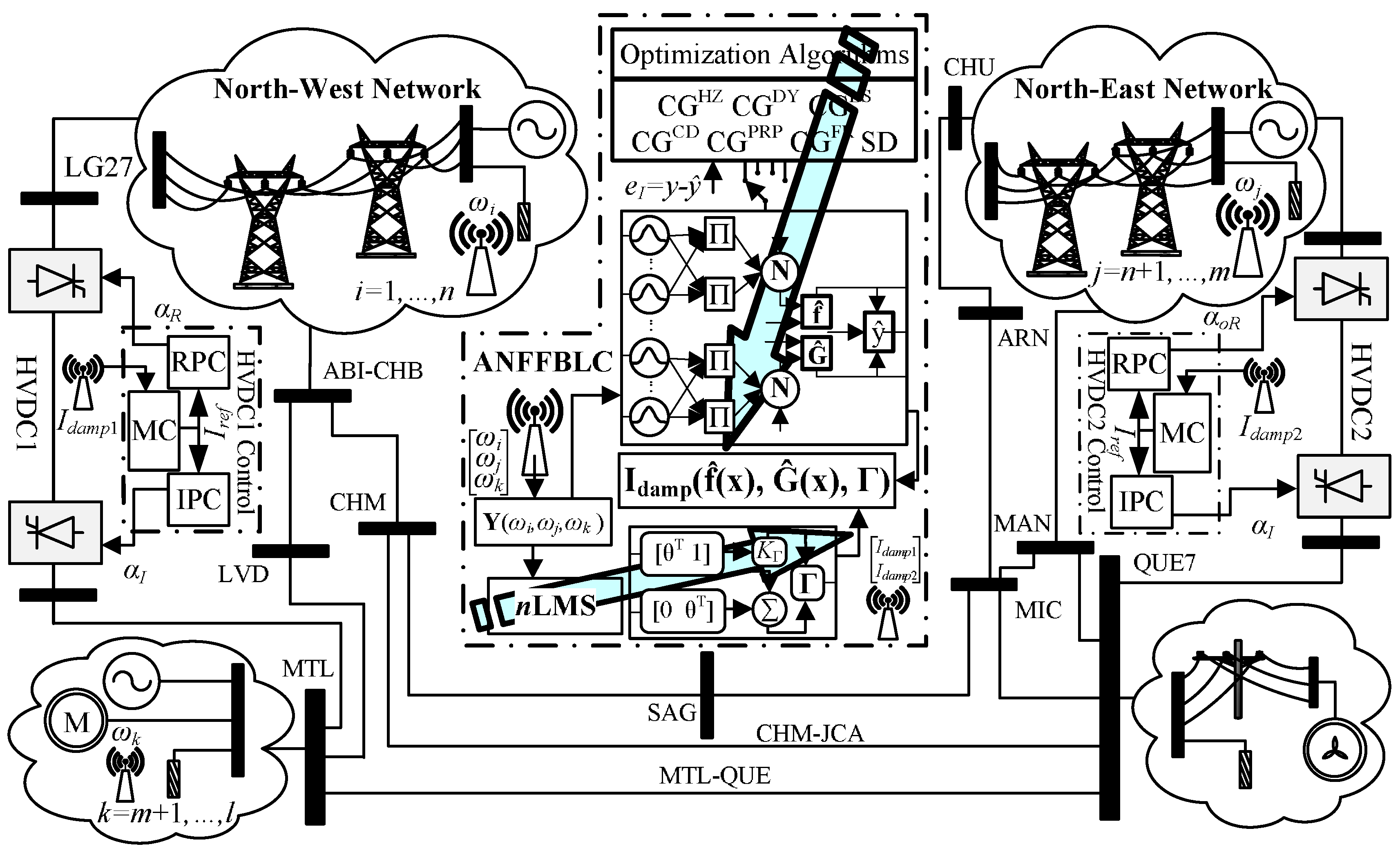
  • The wide area measurement system transmits the actual speed of generators, ω 1 , ω 2 , , ω 7 , to HVDC control.
  • Speed deviations of the generators w.r.t. the swing machine are computed as plant output, y T = [ y 1 y 2 ] , where y 1 = i = 2 5 ( ω i ω 1 ) and y 2 = i = 6 7 ( ω i ω 1 ) .
  • ANFFBLC captures the nonlinear dynamics, f ^ and G ^ , of the power system using y as explained in Section 3.2. The parameters of ANFIS of ANFFBLC are instantaneously optimized through the CG algorithm to minimize the identification error defined in Equation (44).
  • At the same instant, the online estimation generates the appropriate input Γ . The coefficients, Θ , are optimized through the nLMS algorithm to minimize the tracking error of Equation (31).
  • ANFFBLC generates the appropriate control law, u T = [ u 1 u 2 ] that is based on identified functions f ^ and G ^ and optimized Γ as given in Equation (38).
  • The ANFFBLC output constitutes I d a m p 1 and I d a m p 2 for master controls of HVDC Link 1 and Link 2, respectively. The I d a m p modulates the current order for HVDC link using Equation (23).
  • At each pole control, the current order I o r d generates the corresponding ignition delay angle, α , that controls the power flow through the HVDC system
  • During normal operation, I d a m p = 0 , and power flow through the HVDC system is set to a pre-specified value. During perturbed operating conditions, the generators oscillate against each other at a speed different from the set value. The speed deviations are detected by ANFFBLC, and the appropriate damping signal is generated for each HVDC system. The precise power flow control through the HVDC link improves the damping of power oscillations present in the system and improves its stability.

4. Simulation Results and Discussion

The test power system comprises the simplified model of the highly interconnected Hydro-Québec (HQ) power system with two HVDC links implemented in SIMULINK/SimPowerSystem [49]. Seven power plants and loads in different areas are connected through a huge 735-kV transmission network. Major load buses are MTLand QUE with 15,500-MW and 6000-MW loads, respectively. The load includes dynamic load, constant power PQ , constant impedance (Z) and induction motor load. Two HVDC links, each 1000 MW at 500 kV, are installed in the transmission network connecting buses LG27 to MTL and CHU to QUE for bulk power transmission. Sequential AC/DC load flow is used to initialize the system with machine G 1 taken as a swing bus.
The test power system is subjected to various contingencies with different operating conditions, locations and duration. The system response is evaluated through the observation of the following parameters.
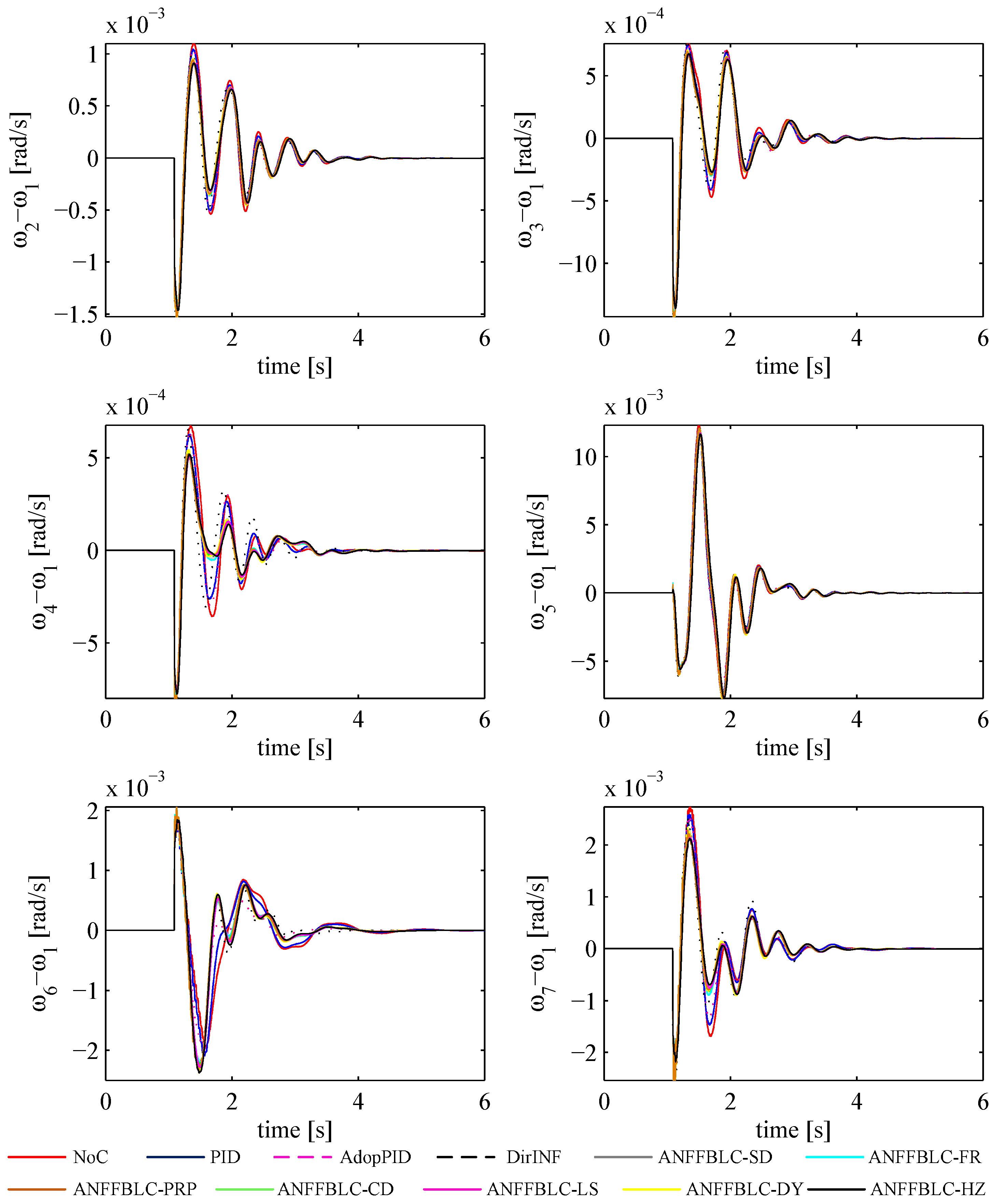
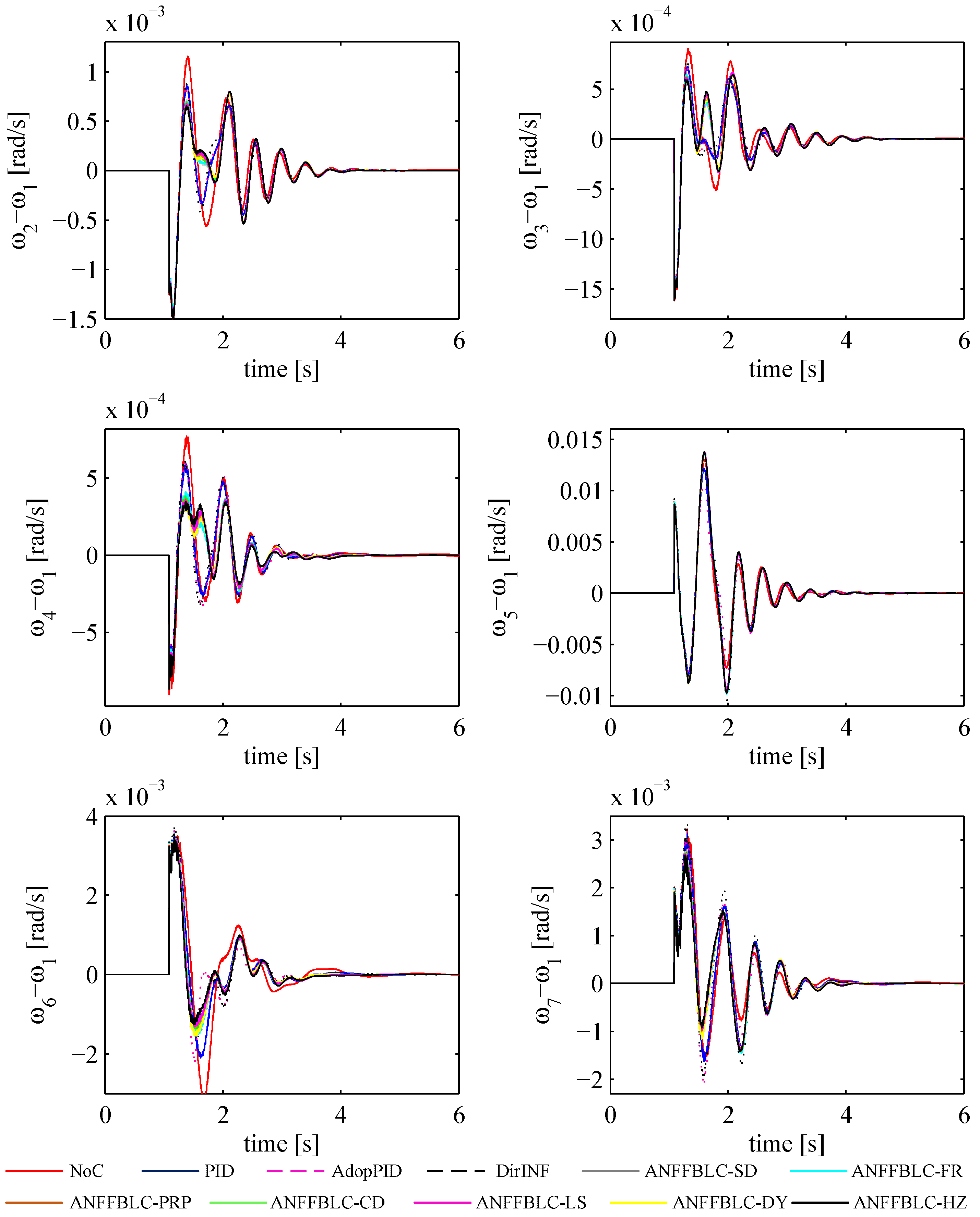
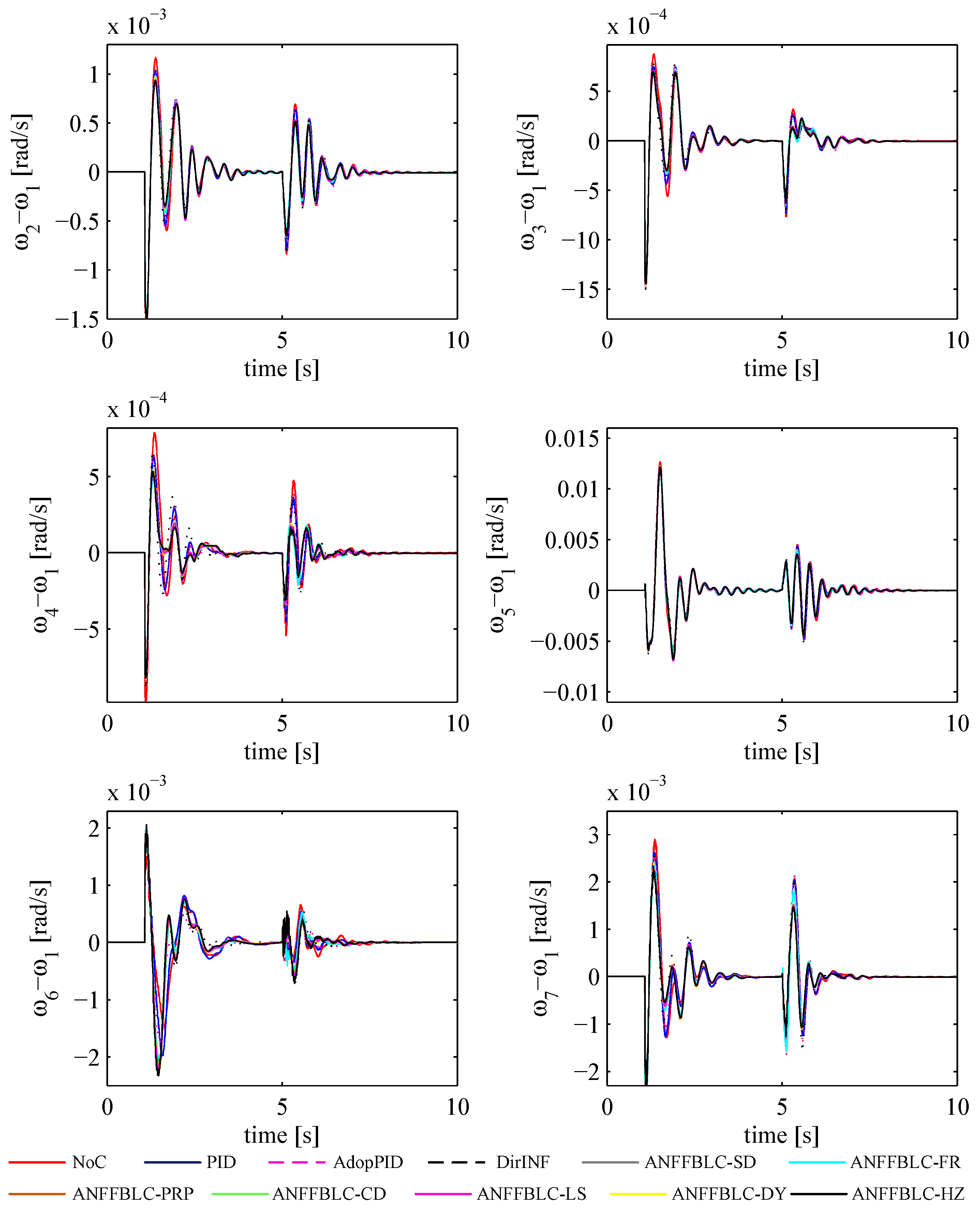
  • Low-frequency oscillations: Observation of over-shoot and settling time for modes with oscillations of generators G 2 to G 6 against the reference generator G 1 i.e., ω i ω 1 , i = 2 , 3 , , 7 .
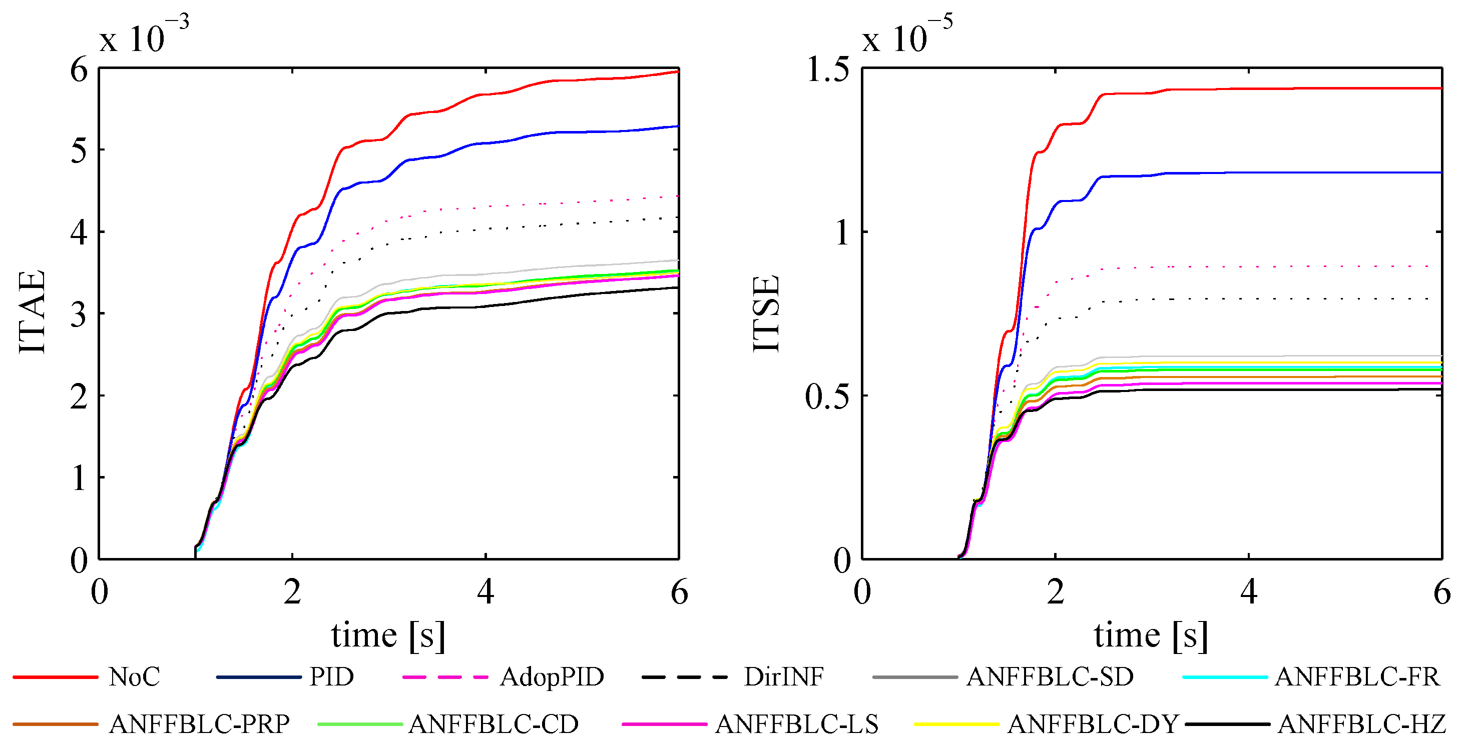
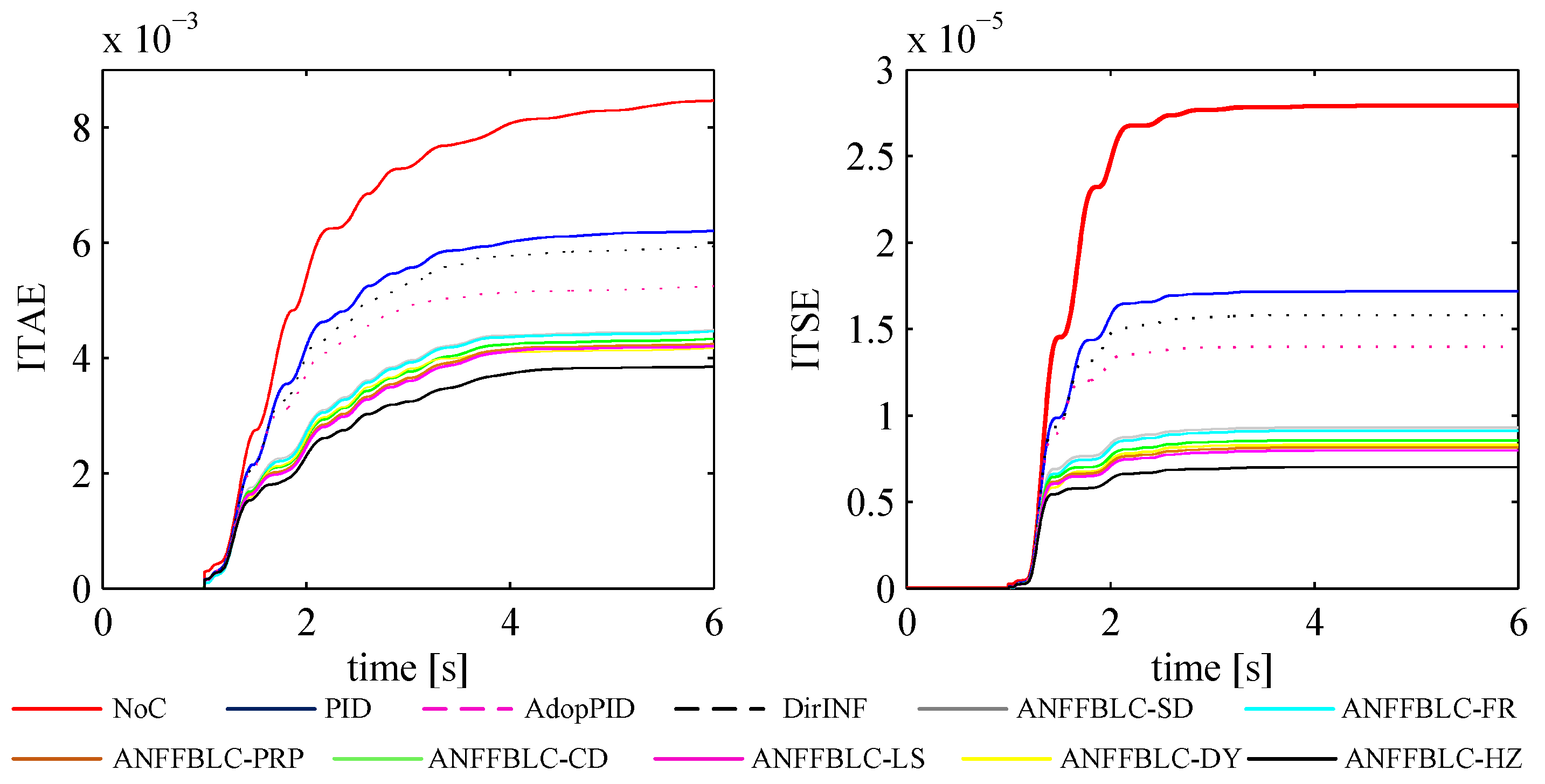
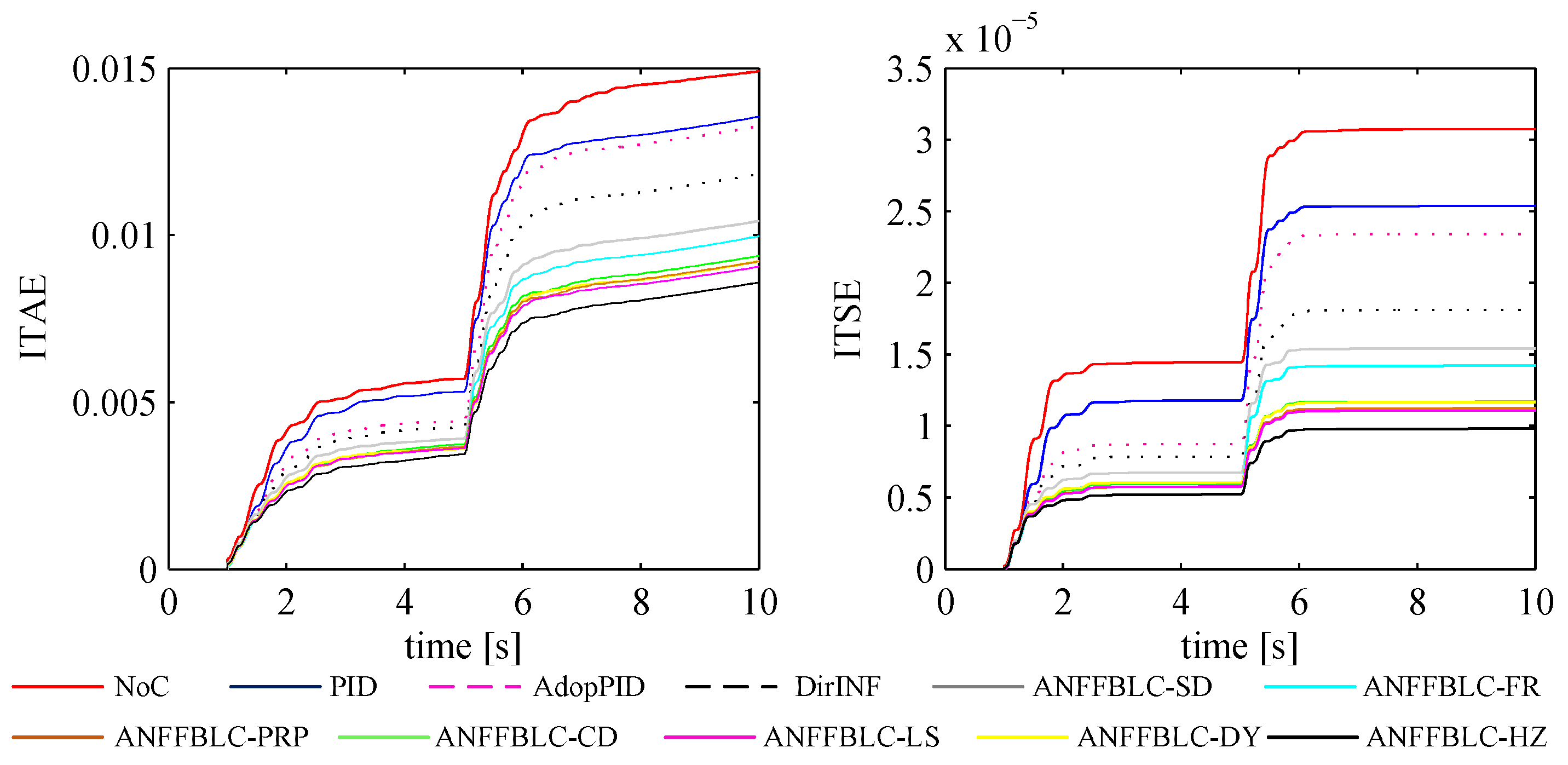
  • Performance indexes: The two used indexes for quantitative measures are Integral of Time-weighted Squared Error (ITSE) and Integral of Time-weighted Absolute Error (ITAE) [50]. For performance indexes, the error is calculated as e p = i = 2 7 ( ω 1 ω i ) .
In each scenario, for the comparison, to verify the effectiveness of damping performance, simulations were carried out with conventional PID control, Adaptive PID (AdapPID) [51], Direct Intelligent Neuro-Fuzzy Control (DirINF) [28], SD-based ANFFBLC and six CG methods.

4.1. Scenario # 1

At t = 1 s, a three-phase to ground fault occurs at HVDC 1 inverter bus MTL. The fault is cleared after 100 ms with a 1000-MW reduction in load at the MTL bus. Targeted oscillation modes are shown in Figure 4. Well-tuned conventional and non-conventional control schemes have competitive damping performance as compared to ANFFBLC with SD and different CG optimization techniques. During the first cycle, the overshoot is reduced by 6–26% with ANFFBLC damping schemes as compared to benchmark controls. For all modes, LFOs are damped completely with all machines settling to steady-state speed. The damping performance of HVDC links with damping control is also assessed through performance indexes. Two performance indexes ITSE and ITAE are shown in Figure 5. The ITSE plot represents time-weighted speed deviation error during the transient-state. The best improvement of 55% in the minimization of the transient-state error is achieved by ANFFBLC-HZ in comparison with PID control, while the ITSE plot of ANFFBLC-FR shows 50% improvement over PID. The ITAE plot represents time-weighted errors persisting for a long time and depicts the damping efforts during the steady-state conditions. The ITAE index for ANFFBLC-HZ shows 36% improvement in damping persistent oscillations as compared to the conventional control. ANFFBLC with SD and CG optimization depicts damping performance in close competition; however, the ANFFBLC-HZ index shows the most effective damping of LFOs. ANFFBLC shows 31–36%, 18–24% and 13–19% improvement in steady-state stability as compared to PID, AdapPID and DirINF, respectively.

4.2. Scenario # 2

The CHM-JCA transmission line is exposed to a three-phase to ground fault at time t = 1 s. The fault is cleared after 120 ms with the permanent outage of the transmission line. Oscillation modes, shown in Figure 6, reveal the more severe nature of the disturbance as post-fault operating conditions have changed. The plots show excessive overshoots with benchmark control schemes, while the ANFFBLC has rapidly dampedthe oscillations, and system settleto steady-state. In some cases, the competitive performance of conventional control is observed during steady-state; however, in the transient-state, 8–16% reduced overshoots are observed with ANFFBLC.
The ITSE and ITAE indexes shown in Figure 7 represent the damping performance comparison. HVDC links with MIMO ANFFBLC have lesser ITSE index values at any time and more flat profiles as compared to the ITSE plot of the benchmark control systems. As compared to conventional PID control, the ITSE plot for ANFFBLC-HZ depicts 63% improvement in damping the transient-state oscillations. The plots for the ANFFBLC schemes get flattened prior to the PID plot that shows the rapid minimization of error by ANFFBLC in the transient-state. Time-weighted index ITAE for ANFFBLC-HZ shows 49% improvement in the steady-state stability of the power system as compared to PID control. ITSE improvement of 46–58%, 38–52% and 30–46% is observed with ANFFBLC as compared to the PID, AdapPID and DirINF control schemes, respectively. While in the steady-state, improvement with ANFFBLC is 28–37%, 20–30% and 10–21%, as compared to the PID, AdapPID and DirINF controllers schemes, respectively. The ANFFBLC-HZ scheme has well contained the LFOs in the transient-state and steady-state conditions and maintains the best performance among different CG methods.

4.3. Scenario # 3

The test power system is subjected to a sequence of faults to investigate the effectiveness and robust nature of the proposed control. A 100-ms three-phase to ground fault occurs at t = 1 s at bus QUE. Another fault arises at bus SAG at time t = 5 s for a duration of 110 ms. Both faults are self-cleared without any structural change in the power system. The response of the system is observed through LFOs modes as shown in Figure 8. In terms of overshoot, the performances of ANFFBLC and conventional control are competitive after the first fault. However, after the second fault, the performance of the ANFFBLC is much more improved than benchmark controllers in terms of overshoot and settling time. The oscillatory behavior of the power system with PID control is observed for different oscillation modes. A better picture of damping performance is described by the performance indexes shown in Figure 9. As perceived by the ITSE plots, transient-state errors are minimized with ANFFBLC and benchmark controllers for both faults. However, ITSE indexes for ANFFBLC schemes have a lesser value and rapidly maintain constant index values during the steady-state condition after the second fault. The ITSE index for ANFFBLC schemes shows overall 39–61%, 34–57% and 15–45% improvement in the minimization of the speed deviation error during transient-state conditions as compared to PID, AdapPID and DirINF controls, respectively. Similar performance trends are observed in ITAE index with 23–35%, 21–34% and 12–26% improvement with ANFFBLC schemes. In Scenario 3, ANFFBLC-HZ has repeated the best damping performance like previous scenarios and shows the most improved transient-state and steady-state conditions.

4.4. Performance Comparison of CG Algorithms

In an application of different CG algorithms in the power system, all methods performed very close to each other and better than conventional control and non-conventional controllers. The damping performance of ANFFBLC with different CG schemes and benchmark controllers is summarized in Table 1. It shows the performance improvement attained by ANFFBLC as compared to conventional and non-conventional control in transient-state and steady-state conditions. The best performance is observed with the ANFFBLC-HZ scheme, while the FR method only performed better than the benchmark controls. The FR scheme suffers a jamming problem in some cases [52], and a modification was proposed in the Polak-Ribière scheme that enables a restart feature to avoid jamming and more rapid convergence as compared to the FR method. The proposed CD method with relaxed constraints is closely related to the FR scheme, and the search directions satisfy the sufficient descent condition under strong Wolfe line search. However, in some particular cases, the CD method may converge to a point where g k 0 [53]. The DY method always generates descent directions and converges globally with the line search satisfying the standard Wolfe condition. The DY method is also susceptible to jamming. The LS method exhibits similar performance as the PRP scheme with exact line search and has an in-built restart feature to avoid the jamming problem. Computation performance of the PRP and LS methods is better than the FR, PRP and DY methods. The HZ method modified the linear CG method of Hestenes and Stiefel that provides sufficient descent with a relaxed accuracy of the line search. In [48], the global convergence is proven to show that for any function and any line search, the sufficient descent condition is satisfied, and the jamming is avoided. That made the ANFFBLC-HZ scheme more robust in computation and provided better optimization of ANFIS parameters to ensure minimized identification error and the best damping performance over the other classical CG algorithms [54].

5. Conclusions

The article presented an MIMO POD controller for multiple HVDC transmission systems. The ANFFBLC schemes effectively modulate the real power flow through the HVDC system to enhance its damping assistance during perturbed conditions. Excited power oscillations under any disturbance are apprehended by the ANFFBLC on the basis of the measured speed signal of generators. SD and six CG algorithms are employed to optimize the parameters of ANFIS that minimize the identification error and captured the updated plant dynamics without a priori knowledge of the system model. The damping performance is investigated through the multi-machine AC/DC power system exposed to the disturbances of different severity. Results obtained for a wide range of operating conditions indicate the improved damping performance of different proposed CG-based ANFFBLC schemes as compared to ANFFBLC-SD, conventional PID control, AdapPID and DirINF. Among CG algorithms, the HZ method shows the best optimization capabilities with strong convergence to optimal minima of the optimization function. Rapid identification of the plant model with the HZ method enables ANFFBLC-HZ to derive the desired control output that effectively damped LFO in the power system. The future work includes the implementation of MIMO nonlinear POD control for multiple HVDC links and FACTS controllers, as well as the investigation of the effect on damping the low-frequency oscillations.

Author Contributions

Saghir Ahmad and Laiq Khan conceived and designed the simulations; Saghir Ahmad performed the simulation; Saghir Ahmad and Laiq khan analyzed the simulation results; Saghir Ahmad wrote the paper.

Conflicts of Interest

The authors declare no conflict of interest.

References

  1. Klein, M.; Rogers, G.J.; Kundur, P. A fundamental study of inter-area oscillations in power systems. IEEE Trans. Power Syst. 1991, 6, 914–921. [Google Scholar] [CrossRef]
  2. Sitnikov, V.; Povh, D.; Retzmann, D.; Teltsch, E. Solutions for large power system interconnections. In Proceedings of the Cigré Conference, Saint Petersburg, Russia, 17–19 September 2003. [Google Scholar]
  3. Rogers, G. Power System Oscillations; Springer: New York, NY, USA, 2012; pp. 7–22. [Google Scholar]
  4. Setreus, J.; Bertling, L. Introduction to HVDC technology for reliable electrical power systems. In Proceedings of the 10th IEEE International Conference on Probabilistic Methods Applied to Power Systems, Rincon, PR, USA, 25–29 May 2008; pp. 1–8. [Google Scholar]
  5. Harnefors, L.; Johansson, N.; Zhang, L.; Berggren, B. Interarea oscillation damping using active-power modulation of multiterminal HVDC transmissions. IEEE Trans. Power Syst. 2014, 29, 2529–2538. [Google Scholar] [CrossRef]
  6. Daryabak, M.; Filizadeh, S.; Jatskevich, J.; Davoudi, A.; Saeedifard, M.; Sood, V.K.; Martinez, J.A.; Aliprantis, D.; Cano, J.; Mehrizi-Sani, A. Modeling of LCC-HVDC systems using dynamic phasors. IEEE Trans. Power Deliv. 2014, 29, 1989–1998. [Google Scholar] [CrossRef]
  7. Li, R.; Bozhko, S.; Asher, G. Frequency control design for offshore wind farm grid with LCC-HVDC link connection. IEEE Trans. Power Electron. 2008, 23, 1085–1092. [Google Scholar] [CrossRef]
  8. MESSINA. Damping of low-frequency interarea oscillations using HVDC modulation and SVC voltage support. Electr. Power Compon. Syst. 2003, 31, 389–402. [Google Scholar]
  9. Badran, S.M.; Choudhry, M.A. Design of modulation controllers for AC/DC power systems. IEEE Trans. Power Syst. 1993, 8, 1490–1496. [Google Scholar] [CrossRef]
  10. Pipelzadeh, Y.; Chaudhuri, B.; Green, T.C. Coordinated damping control through multiple HVDC systems: A decentralized approach. In Proceedings of the 2011 IEEE Power and Energy Society General Meeting, San Diego, CA, USA, 24–29 July 2011; pp. 1–8. [Google Scholar]
  11. Mao, X.; Yao, Z.; Lin, G.; Wu, X. Researches on coordinated control strategy for inter-area oscillations in AC/DC hybrid grid with multi-infeed HVDC. In Proceedings of the 2005 IEEE/PES Transmission and Distribution Conference and Exhibition: Asia and Pacific, Dalian, China, 18 August 2005; pp. 1–6. [Google Scholar]
  12. Rahman, H.L.; Khan, B.H. Stability improvement of power system by simultaneous AC-DC power transmission. Electr. Power Syst. Res. 2008, 78, 756–764. [Google Scholar] [CrossRef]
  13. Hammons, J.; Yeo, R.L.; Gwee, C.L.; Kacejko, P.A. Enhancement of power system transient response by control of HVDC converter power. Electr. Mach. Power Syst. 2000, 28, 219–241. [Google Scholar]
  14. Cai, H.; Qu, Z.; Gan, D. A nonlinear robust HVDC control for a parallel AC/DC power system. Comput. Electr. Eng. 2003, 29, 135–150. [Google Scholar] [CrossRef]
  15. Mc Namara, P.; Negenborn, R.R.; De Schutter, B.; Lightbody, G. Optimal coordination of a multiple HVDC link system using centralized and distributed control. IEEE Tran. Control Syst. Technol. 2013, 21, 302–314. [Google Scholar] [CrossRef]
  16. Preece, R.; Milanovic, J.V.; Almutairi, A.M.; Marjanovic, O. Damping of inter-area oscillations in mixed AC/DC networks using WAMS based supplementary controller. IEEE Trans. Power Syst. 2013, 28, 1160–1169. [Google Scholar] [CrossRef]
  17. Lascu, C.; Jafarzadeh, S.; Fadali, M.S.; Blaabjerg, F. Direct torque control with feedback linearization for induction motor drives. IEEE Trans. Power Electron. 2017, 32, 2072–2080. [Google Scholar] [CrossRef]
  18. Khan, L.; Lo, K.L. Hybrid micro-GA based FLCs for TCSC and UPFC in a multi-machine environment. Electr. Power Syst. Res. 2006, 76, 832–843. [Google Scholar] [CrossRef]
  19. Song, G.; Song, G.; Longman, R.W.; Mukherjee, R. Integrated sliding-mode adaptive-robust control. IEE Proc. Control Theory Appl. 1999, 146, 341–347. [Google Scholar] [CrossRef]
  20. Eriksson, R.; Knazkins, V.; Söder, L. Coordinated control of multiple HVDC links using input–output exact linearization. Electr. Power Syst. Res. 2010, 80, 1406–1412. [Google Scholar] [CrossRef]
  21. Lee, D.; Kim, H.J.; Sastry, S. Feedback linearization vs. adaptive sliding mode control for a quadrotor helicopter. Inter. J. Control Autom. Syst. 2009, 7, 419–428. [Google Scholar] [CrossRef]
  22. Malik, O.P. Adaptive control of synchronous machine excitation. In Microprocessor-Based Control Systems; Sinha, N.K., Ed.; Springer: Dordrecht, The Netherlands, 1986; pp. 61–79. [Google Scholar]
  23. Yeşildirek, A.; Lewis, F.L. Feedback linearization using neural networks. Automatica 1995, 31, 1659–1664. [Google Scholar] [CrossRef]
  24. Arif, J.; Ray, S.; Chaudhuri, B. MIMO feedback linearization control for power systems. Int. J. Electr. Power Energy Syst. 2013, 45, 87–97. [Google Scholar] [CrossRef]
  25. Khan, L.; Ahmed, N.; Lozano, C. GA neuro-fuzzy damping control system for UPFC to enhance power system transient stability. In Proceedings of the 7th International Multi Topic Conference (INMIC 2003), Islamabad, Pakistan, 8–9 December 2003; pp. 276–282. [Google Scholar]
  26. Mitra, S.; Hayashi, Y. Neuro-fuzzy rule generation: Survey in soft computing framework. IEEE Trans. Neural Netw. 2000, 11, 748–768. [Google Scholar] [CrossRef] [PubMed]
  27. Azar, A.T. Adaptive Neuro-Fuzzy Systems. In Fuzzy Systems; Azar, A.T., Ed.; IN-TECH: Vienna, Austria, 2010; pp. 85–110. [Google Scholar]
  28. Shi, M.; Mizumoto, M. Some considerations on conventional neuro-fuzzy learning algorithms by gradient descent method. Fuzzy Sets Syst. 2000, 112, 51–63. [Google Scholar] [CrossRef]
  29. Shewchuk, J.R. An Introduction to the Conjugate Gradient Method without the Agonizing Pain; Carnegie Mellon University: Pittsburgh, PA, USA, 1994. [Google Scholar]
  30. Saini, L.M.; Soni, M.K. Artificial neural network-based peak load forecasting using conjugate gradient methods. IEEE Trans. Power Syst. 2002, 17, 907–912. [Google Scholar] [CrossRef]
  31. Liang, N.Y.; Huang, G.B.; Saratchandran, P.; Sundararajan, N. A fast and accurate online sequential learning algorithm for feedforward networks. IEEE Trans. Neural Netw. 2006, 17, 1411–1423. [Google Scholar] [CrossRef] [PubMed]
  32. Ahmad, S.; Khan, L. Adaptive feedback linearization based HVDC damping control paradigm for power system stability enhancement. In Proceedings of the IEEE 2016 International Conference on Emerging Technologies (ICET), Islamabad, Pakistan, 18–19 October 2016; pp. 1–6. [Google Scholar]
  33. Marino, R.; Tomei, P. Robust stabilization of feedback linearizable time-varying uncertain nonlinear systems. Automatica 1993, 29, 181–189. [Google Scholar] [CrossRef]
  34. Slock, D.T. On the convergence behavior of the LMS and the normalized LMS algorithms. IEEE Trans. Signal Process. 1993, 41, 2811–2825. [Google Scholar] [CrossRef]
  35. Ahmad, S.; Khan, L. A self-tuning NeuroFuzzy feedback linearization-based damping control strategy for multiple HVDC links. Turk. J. Electr. Eng. Comput. Sci. 2017, 25, 913–938. [Google Scholar] [CrossRef]
  36. Sauer, P.W.; Pai, M.A. Power System Dynamics and Stability, 1st ed.; Pearson Education: Dehli, India, 1998. [Google Scholar]
  37. Yazdani, A.; Iravani, R. Voltage-Sourced Converters in Power Systems: Modeling, Control, and Applications; John Wiley & Sons Inc.: Hoboken, NJ, USA, 2010. [Google Scholar]
  38. Kundur, P. Power System Stability and Control, 3rd ed.; McGraw-Hill: New York, NY, USA, 1994; pp. 463–580. [Google Scholar]
  39. Arrillaga, J.; Liu, Y.H.; Watson, N.R. Flexible Power Transmission: The HVDC Options; John Wiley & Sons Ltd.: Chichester, UK, 2007. [Google Scholar]
  40. Slotine, J.J.; Li, W. Applied Nonlinear Control; Prentice-Hall: Englewood Cliffs, NJ, USA, 1991; pp. 207–271. [Google Scholar]
  41. Labiod, S.; Boucherit, M.S.; Guerra, T.M. Adaptive fuzzy control of a class of MIMO nonlinear systems. Fuzzy Sets Syst. 2005, 151, 59–77. [Google Scholar] [CrossRef]
  42. Nocedal, J.; Wright, S.J. Numerical Optimization, 2nd ed.; Springer: New York, NY, USA, 2006; pp. 101–134. [Google Scholar]
  43. Fletcher, R.; Reeves, C.M. Function minimization by conjugate gradients. Comput. J. 1964, 7, 149–154. [Google Scholar] [CrossRef]
  44. Zhang, L.; Zhou, W.; Li, D.H. A descent modified Polak-Ribière-Polyak conjugate gradient method and its global convergence. IMA J. Numerical Anal. 2006, 26, 629–640. [Google Scholar] [CrossRef]
  45. Fletcher, R. Practical Methods of Optimization, 2nd ed.; John Wiley & Sons Ltd.: Chichester, UK, 1987; pp. 80–94. [Google Scholar]
  46. Liu, Y.; Storey, C. Efficient generalized conjugate gradient algorithms, part 1: Theory. J. Optim. Theory Appl. 1991, 69, 129–137. [Google Scholar] [CrossRef]
  47. Dai, Y.H.; Yuan, Y. A nonlinear conjugate gradient method with a strong global convergence property. SIAM J. Optim. 1999, 10, 177–182. [Google Scholar] [CrossRef]
  48. Hager, W.W.; Zhang, H. A new conjugate gradient method with guaranteed descent and an efficient line search. SIAM J. Optim. 2005, 16, 170–192. [Google Scholar] [CrossRef]
  49. Ahmad, S.; Khan, L. Adaptive feedback linearization control for power oscillations damping in AC/DC power system. In Proceedings of the IEEE 13th International Conference on Frontiers of Information Technology (FIT), Islamabad, Pakistan, 14–16 December 2015; pp. 199–204. [Google Scholar]
  50. Solihin, M.I.; Tack, L.F.; Kean, M.L. Tuning of PID controller using particle swarm optimization (PSO). Int. J. Adv. Sci. Eng. Inf. Technol. 2011, 1, 458–461. [Google Scholar] [CrossRef]
  51. Ali, S.; Khan, M.H.; Raja, A.A. TCSC based online adaptive control for improving damping in multimachine power system. In Proceedings of the IEEE International Conference on Energy Systems and Policies (ICESP), Islamabad, Pakistan, 24–26 November 2014; pp. 1–5. [Google Scholar]
  52. Powell, M.J. Restart procedures for the conjugate gradient method. Math. Program. 1977, 12, 241–254. [Google Scholar] [CrossRef]
  53. Dai, Y.; Han, J.; Liu, G.; Sun, D.; Yin, H.; Yuan, Y.X. Convergence properties of nonlinear conjugate gradient methods. SIAM J. Optim. 2000, 10, 345–358. [Google Scholar] [CrossRef]
  54. Hager, W.W.; Zhang, H. A survey of nonlinear conjugate gradient methods. Pac. J. Optim. 2006, 2, 35–58. [Google Scholar]
Figure 1. The Line Commutated Converter (LCC)-HVDC system average model implementation and control.
Energies 10 00819 g001
Figure 2. AC/DC power system with the closed-loop control system.
Energies 10 00819 g002
Figure 3. MIMO neuro-fuzzy identification architecture.
Energies 10 00819 g003
Figure 4. Relative speed deviations for various machines with fault at bus MTL and a 1000-MW load reduction.
Energies 10 00819 g004
Figure 5. Performance indexes with fault at bus MTL and a 1000-MW load reduction.
Energies 10 00819 g005
Figure 6. Relative speed deviations for various machines with the fault at line CHM-JCA and line outage.
Energies 10 00819 g006
Figure 7. Performance indexes with fault at line CHM-JCA and line outage.
Energies 10 00819 g007
Figure 8. Relative speed deviations for various machines with a sequence of faults at buses QUE and SAG.
Energies 10 00819 g008
Figure 9. Performance indexes with a sequence of faults at buses QUE and SAG .
Energies 10 00819 g009
Table 1. Performance improvement of ANFFBLC as compared to conventional control.
ScenarioPerformance%Age Improvement AdapPID, DirINF and ANFFBLC w.r.t. PID
IndexAdapPIDDirINFSDFRCDDYPRPLSHZ
1ITAE162131333335353536
ITSE243347505151535455
2ITAE92028283031323337
ITSE122346475052535458
3ITAE21323263132323335
ITSE82939445454565661

