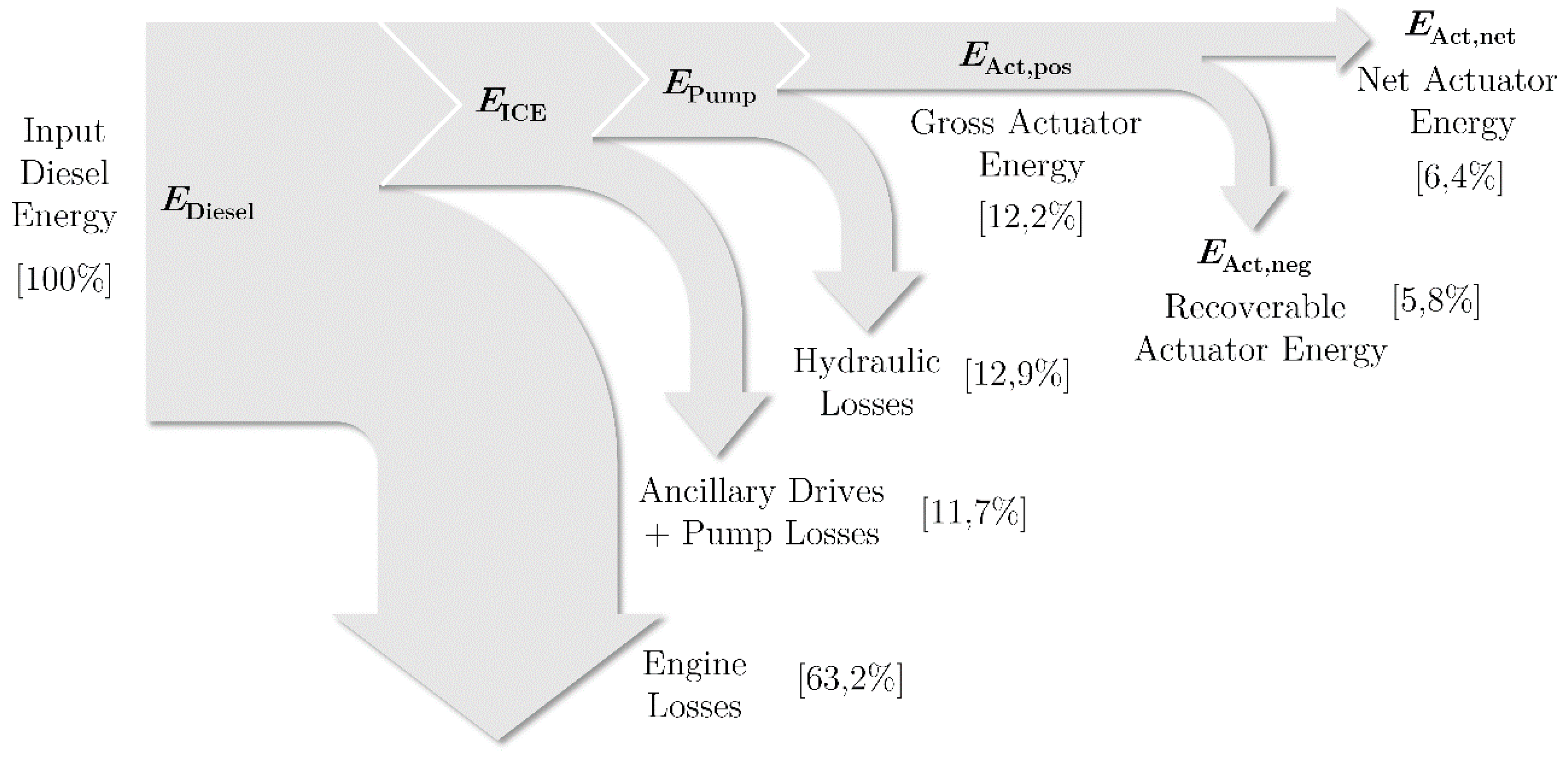
The exact reasons for these losses and their importance can be derived by analysing the individual machine subsystems and their interactions with one another in more detail. Let us begin by discussing the engine.
2.1. Engine
In theory, an engine can reach an efficiency of up to 100%, as the chemical input and mechanical output energies are both ordered and of the same quality, i.e., have the same exergy [
3,
4]. Unfortunately, converting chemical energy directly into mechanical work proves difficult and the fuel must first be ignited in an unconstrained chemical reaction generating heat and losses. As a result, engines specifically designed and optimised to work at a specific operating point can push their peak efficiency into a region of 45–50% but the typical units found in construction machinery display maximum efficiencies of just over 40% [
5]. This value changes considerably depending on the load, i.e., torque, and speed at which the engine operates. An exemplary internal combustion engine (ICE) efficiency map is shown in
Figure 3a.
The map is bounded by the full load line
, which corresponds to the maximum torque or power the ICE can generate at each rotation speed. If the ICE is operated along this line, no additional acceleration torque is available. Load torques above this value lead to a deceleration of the output shaft. Only above the minimum rotation speed
of about 800 rpm can an engine generate enough mechanical power to overcome its internal losses. Typical units provide a substantial acceleration torque at rotation speeds larger than 1000 rpm [
6]. As the speed increases and more power can be generated, the efficiency starts improving. However, higher speeds also lead to increased friction losses and allow less time for the reactants to mix during the combustion process. As a result, efficiency first increases and then begins decreasing with speed. The so-called sweet spot in the contour plot is therefore usually located in the lower to mid-speed range just below the full load line.
Efficiency maps are characterised by curves of constant power, hyperbolas. Not every power curve passes through the optimal operating region, indicating that the unit can only function efficiently within a certain power range. When selecting an engine for a specific application, in this case an excavator, the designer must take into account the peak power demand of the hydraulic system driven by the engine. In most engines, the rotation speed
, at which maximum power is available, is considerably higher than the speed
at which maximum efficiency is attained. In order to deliver peak power and thereby avoid having to change the engine speed during a working cycle, standard excavators are frequently operated at a fixed engine speed, namely
. During such a cycle, the load pressure and pump displacement will vary constantly, leading to fluctuations in the load torque shown in grey in
Figure 3a. This results in frequent part loading and therefore inefficient engine utilisation [
7].
Thinking in terms of absolute efficiency can be misleading, as fuel consumption is, in fact, the quantity that really matters. The Willans approximation, illustrated in
Figure 3b, is another method of plotting engine performance and reveals some interesting aspects that are not so evident from the contour plotted efficiency map [
8]. The fuel consumption
of an engine at a constant speed increases approximately linearly with its output power. For most diesel engines, this proportionality factor takes on a value of about 0.22 L/kWh [
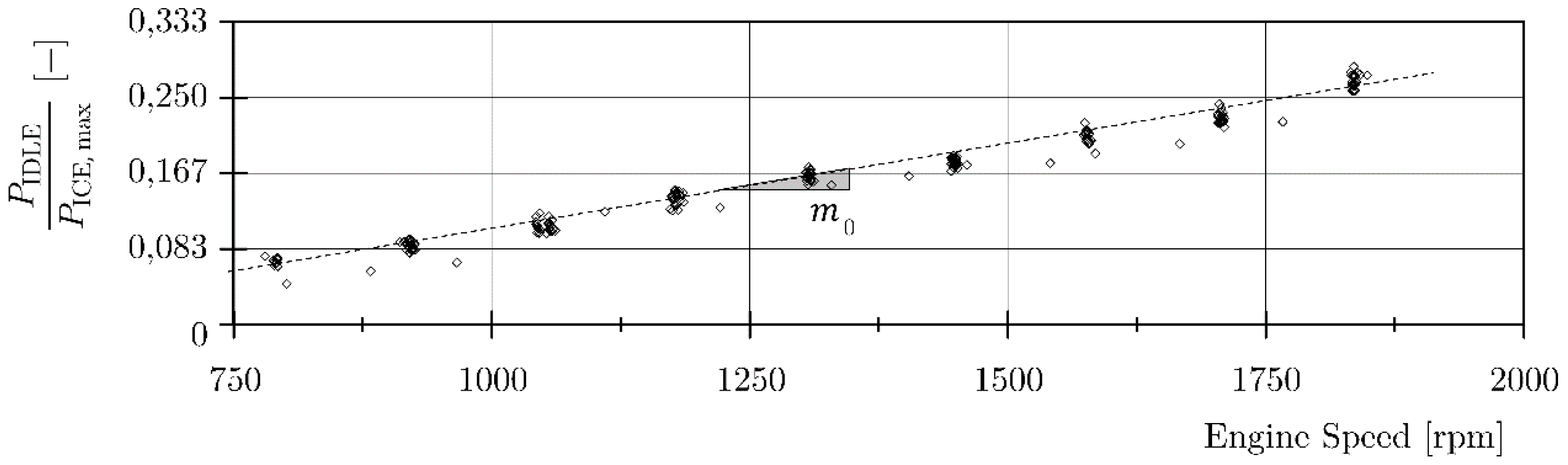
9]. In other words, each additional kW of output power results in the same increase in the fuel consumption rate, regardless of the current operating point. What this actually means is that the engine’s differential efficiency is actually a constant with a value of 42%. The Willans lines also show that an engine delivering no power still consumes fuel due to its parasitic losses. This is referred to as the idle fuel consumption
and largely depends on the engine size
, the number of pistons/cylinders and rotation speed
. In general, larger engines and higher rotation speeds lead to higher parasitic losses and therefore an increase in idle fuel consumption.
According to Rohde-Brandenburger, in the case of a turbocharged diesel engine, the Willans approximation can be expressed as follows [
8]:
with
This is in fact the reason why cars with engine start–stop systems reduce fuel consumption. Similarly, this explains the real advantage of the concepts referred to as engine downsizing and downspeeding. It is not due to the widely cited claim that the thermodynamic efficiency of the engine improves when operating at higher loads and smaller displacements, but rather that the idle fuel consumption of a downsized or downsped engine is lower [
9,
10]. This concept reveals invaluable information regarding how much the fuel consumption of a vehicle can be improved without making changes to the engine. For example, in the case of an average passenger vehicle with a four cylinder engine, the idle fuel consumption is responsible for up to 50% of the total fuel consumption in the new European driving cycle (NEDC). This would mean that the maximum fuel reduction achievable, by designing a new vehicle with theoretically zero mass and zero wind resistance but without any changes to the engine and gearbox, is only 50% [
9]. This highlights the importance of using smaller engines operating at lower speeds.
These observations have important consequences for the energy management strategies in hybrid vehicles. When an engine is already running, the decision to charge the battery or accumulator using the engine can be made without regarding the current operating point because the differential efficiency is constant [
11]. Only when the engine is off does the decision to charge lead to additional losses due to idling.
Reducing engine losses has not been one of the main concerns of excavator manufacturers in recent years. In the late 20th century, studies proved that the particulate matter (PM), carbon monoxide (CO) and nitrous oxides (NO
X) formed during the combustion of diesel fuel, are all detrimental to human health [
12,
13,
14]. In an attempt to improve the air quality in cities and towns, governments introduced a set of stringent diesel emission standards in the 1990s. The initial TIER 1–3 standards (in Europe Stage I–III), phased in between 1998 and 2008, were met using advanced engine designs and basically no or very simple exhaust gas after-treatment methods. With the introduction of the TIER 4 interim and final (European Stage IIIB and IV) standards, which were phased in from 2008 to 2015, manufacturers first agreed to decrease PM and then NO
X emissions by a further 90%. Meeting these standards was considerably more difficult.
Today’s excavators and other off-highway machines use expensive after-treatment systems with diesel oxidation catalysts (DOC) and diesel particulate filters (DPF). This has led to increased costs and a further reduction in the available installation space around the engine. As explained by Filla, the way in which emissions tests are currently conducted has also given OEMs (Original Equipment Manufacturers) little or no incentive to introduce efficient downspeed engines with hybrid technologies [
15]. The official non-road transient cycle (NRTC), used to evaluate engine emissions, uses a predetermined set of engine speeds and torques, which may not even match the actual engine operation in a machine. As a result, a machine with an advanced engine management system would be no different to a standard unit in regard to the current engine emissions regulations.
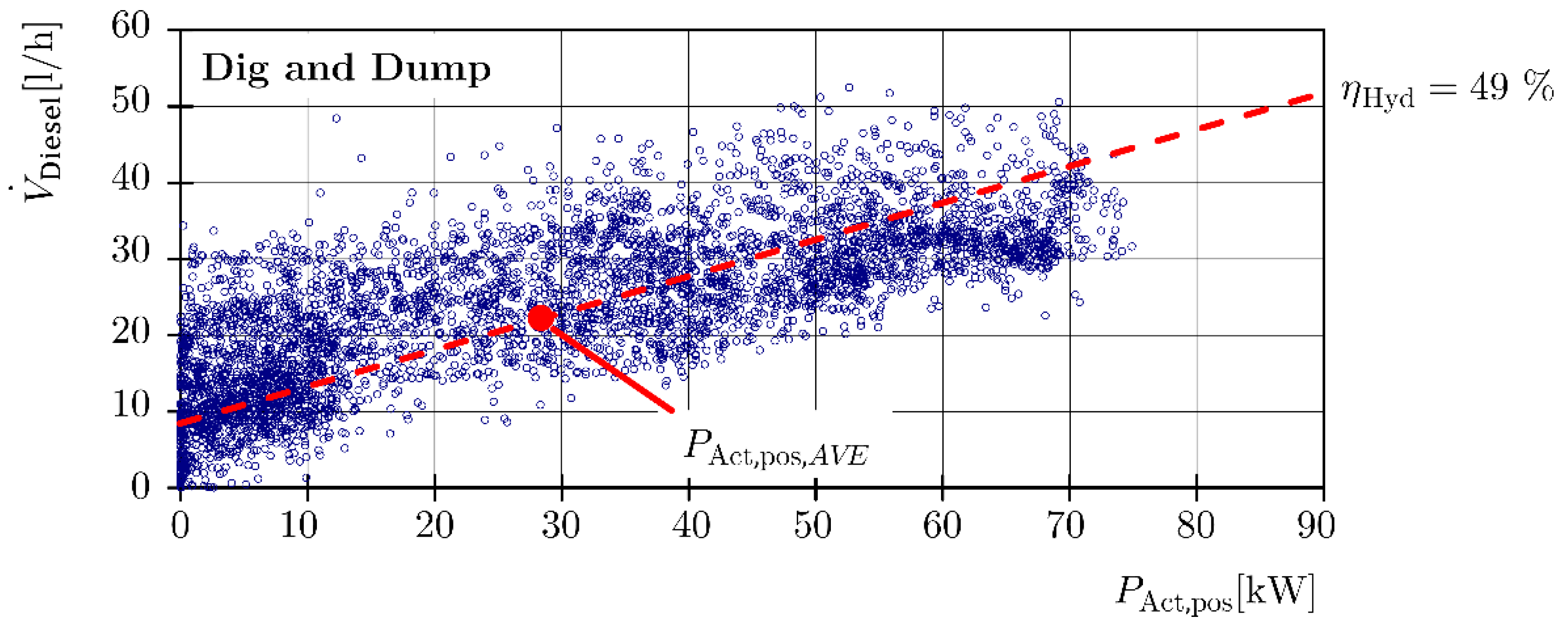
All the aspects mentioned above relate to quasi-static engine performance. As shown in
Figure 4 the effect of dynamic engine loading should not and cannot be neglected. In any typical excavator duty cycle, the engine load fluctuates rapidly and the engine must be able to respond quickly to these load changes to avoid stalling or excessive drops in rotation speed [
16].
Depending on the extent of these transients, fuel consumption can fluctuate considerably from the quasi-static descriptions in
Figure 3. Research has, in fact, shown that up to 50% of emissions are caused by transient loads [
17,
18]. As a result, newer TIER 4 engines do not have the same response that the older TIER 3 engines had. This is especially evident at lower engine speeds and is an important issue that will affect the design of newer mobile hydraulic systems.
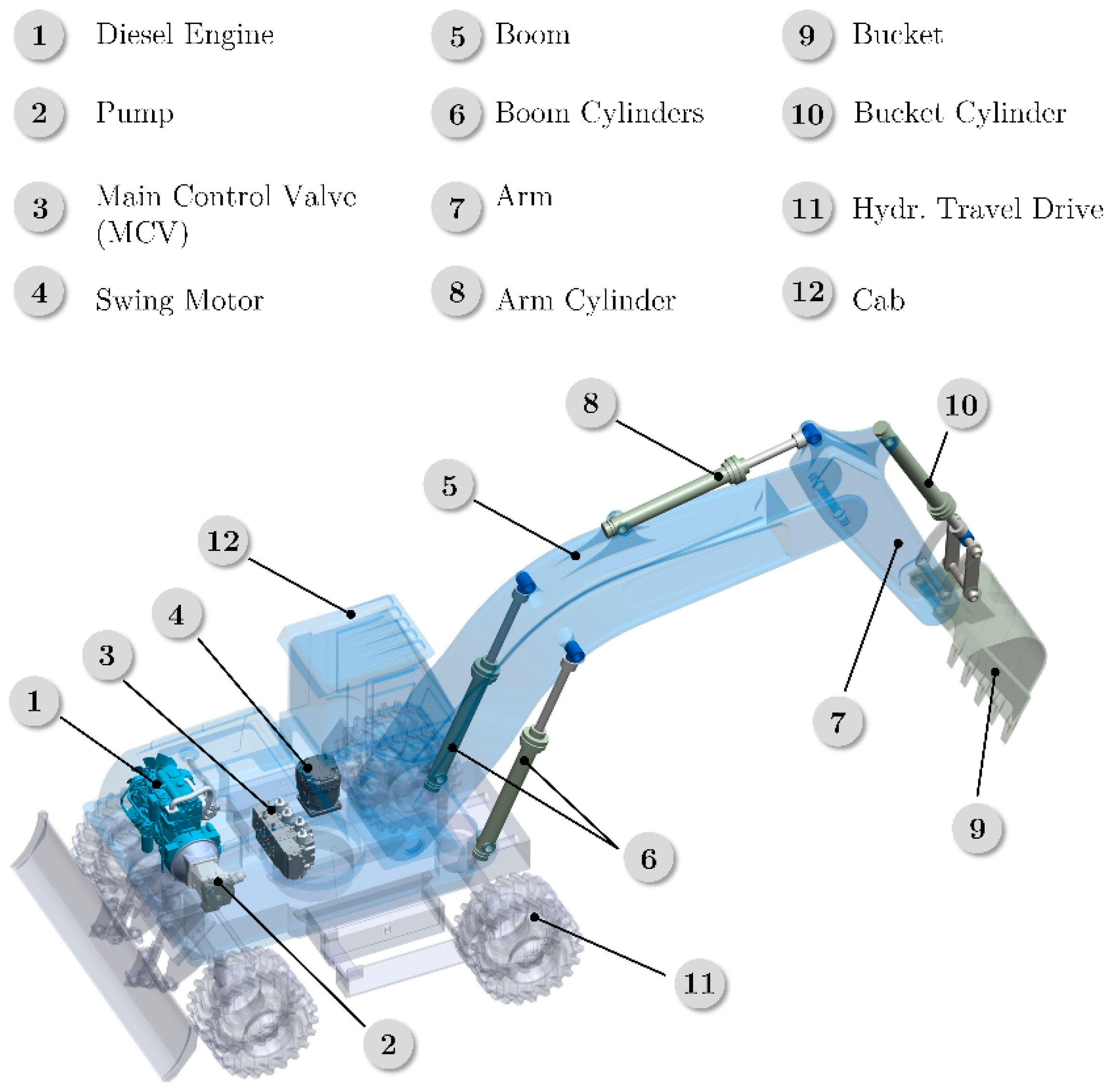
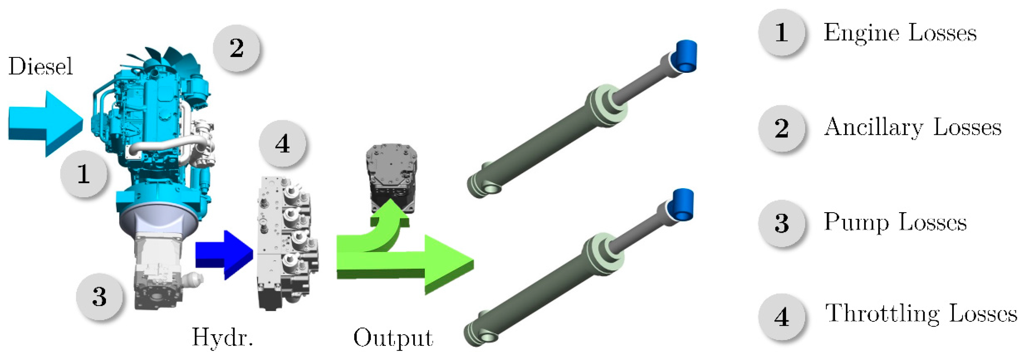
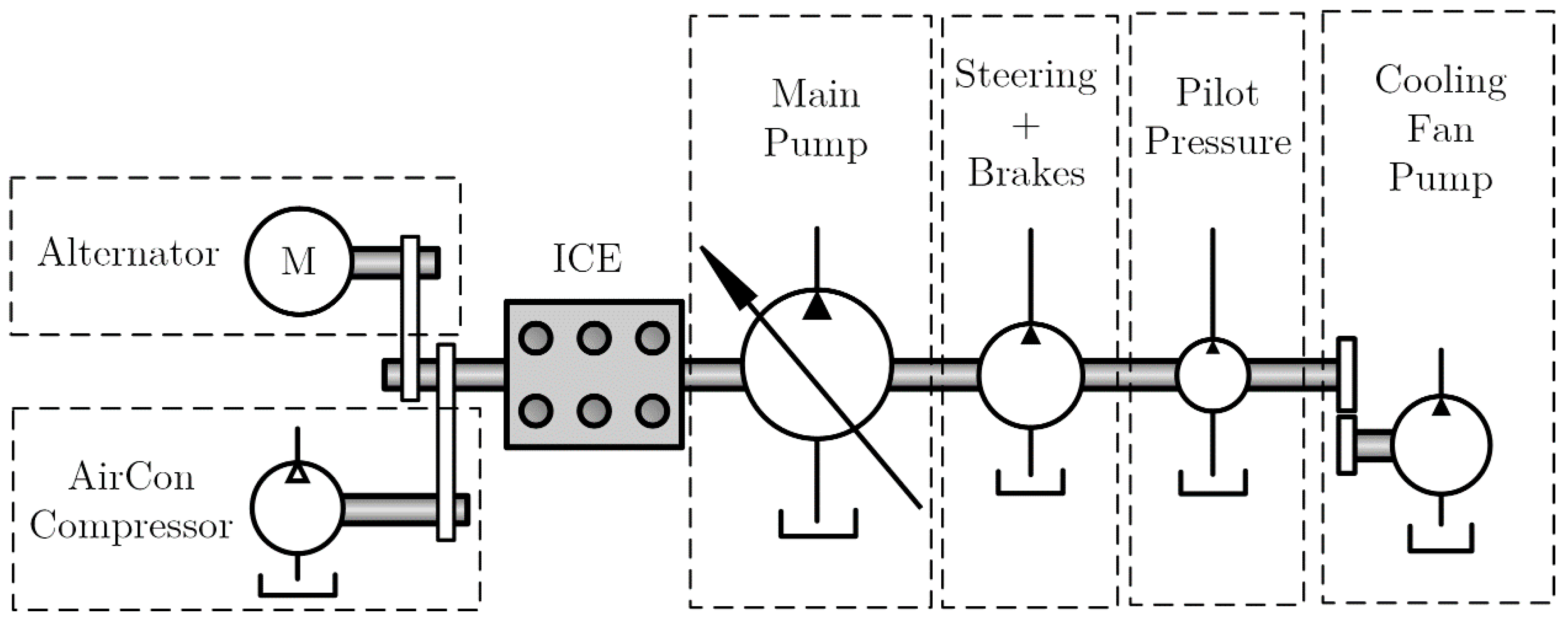
The mechanical power generated by the engine, must now be distributed to the individual hydraulic actuators. This takes us to the machine’s hydraulic system.
2.2. Hydraulic System
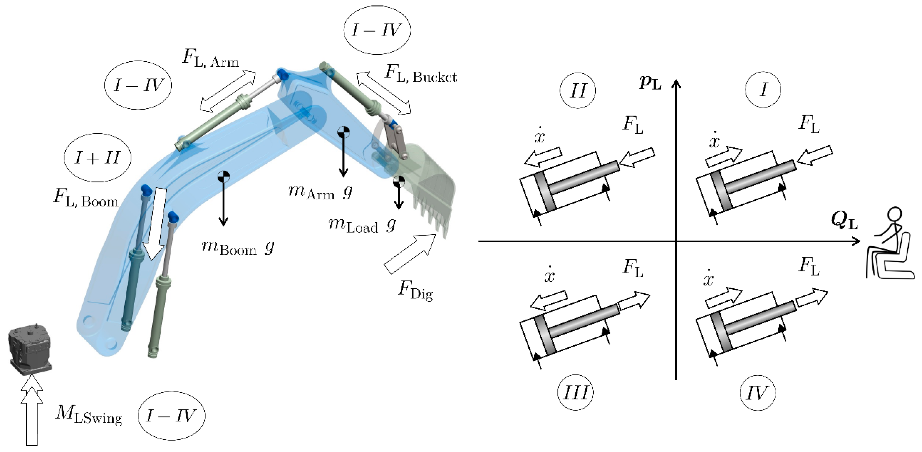
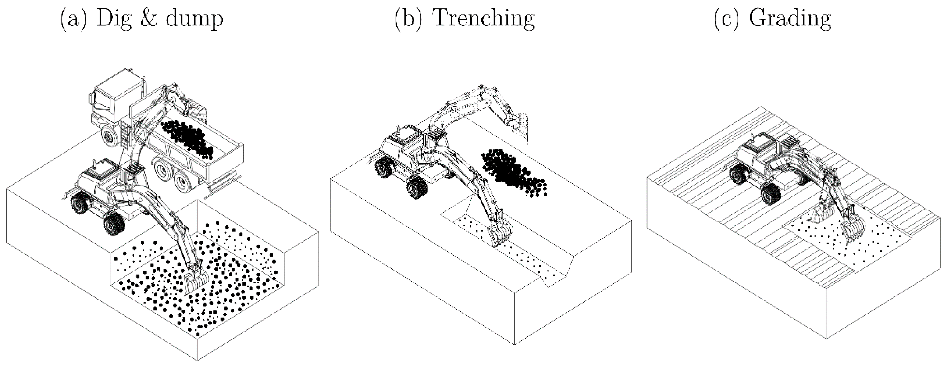
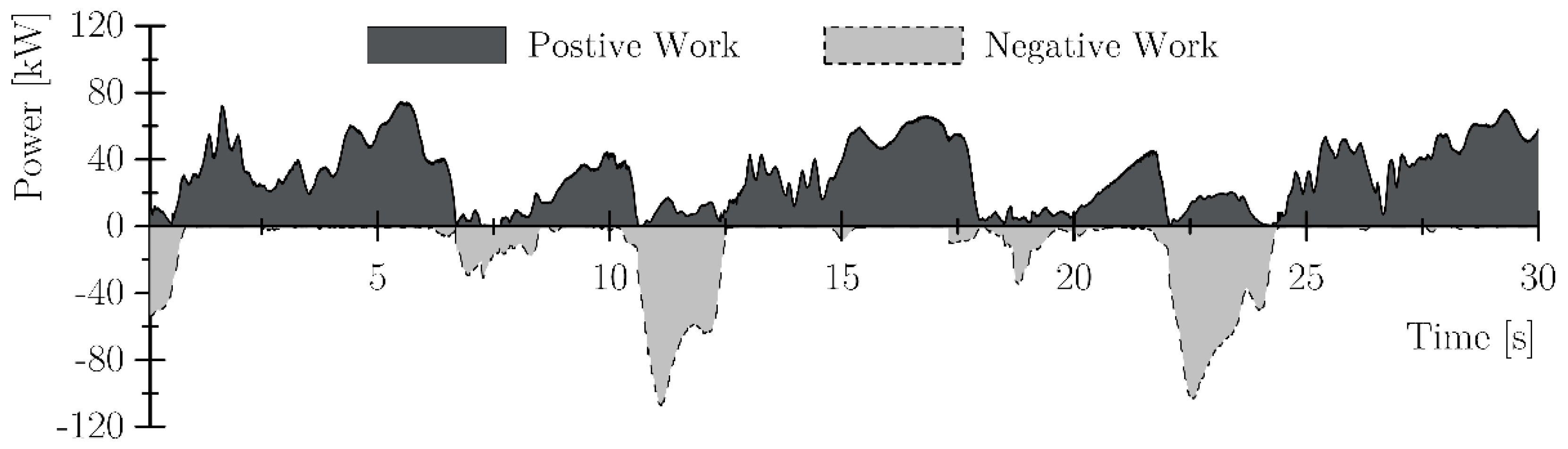
The way in which the hydraulic actuators interact with the external environmental load is particularly complex. Not only are the force and velocity demands of each actuator completely different, they also vary independently of each other depending on the operator’s commands. Some actuators may require high force and low velocity (high pressure, low flow) while others require low force and high velocity (low pressure, high flow).
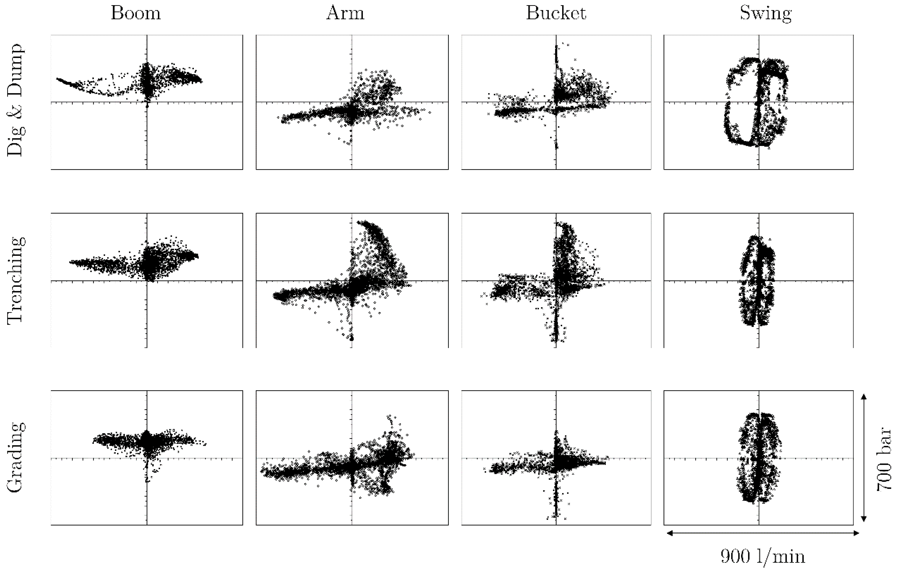
Figure 5 illustrates the load situation for the actuators making up the implement structure. The x-axis shows the flow required by each actuator (
) and can be interpreted as the operator’s input to the system. The y-axis shows the force or load pressure (
) experienced by the actuator and is a direct consequence of the surroundings, cf. Equations (3)–(5).
In the case of the linear actuators, the force acting on them is due to both the weight of the attached structure and the external forces present during digging and other operations. Inertial forces caused during acceleration play a less important role. Depending on the movements, each actuator experiences either a resistive force opposing its motion (Quadrants I and III) or an assistive force aiding its motion (Quadrants II and IV). Consequently, in quadrants I and III, the actuator must be actively supplied with power, while, in quadrants II and IV, the actuators can actually supply power to the system.
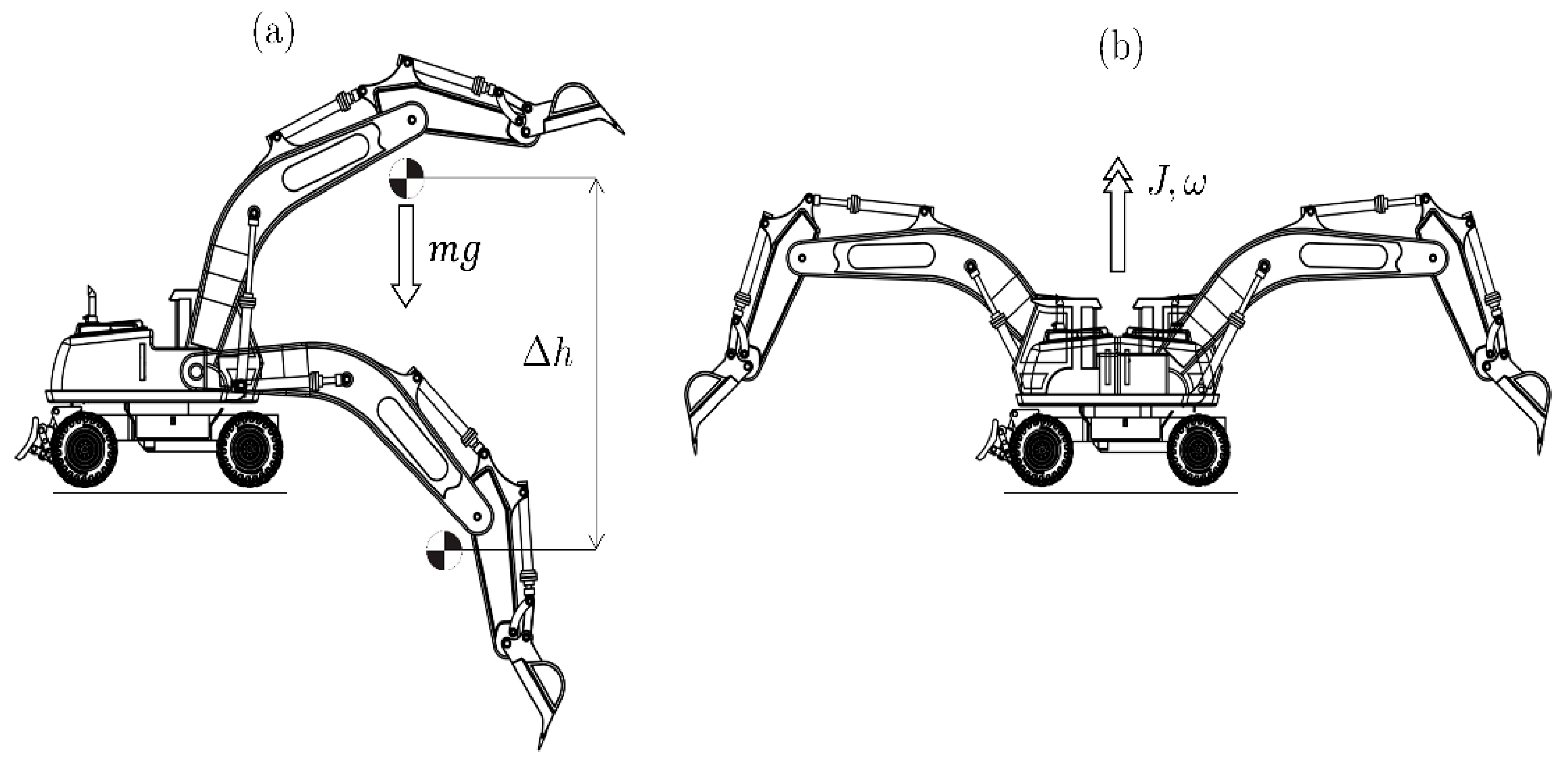
Due to the kinematic arrangement and large weight of the implement structure, the boom cylinders almost exclusively operate in load quadrants I and II. In contrast, the magnitude and direction of the load acting on the arm and bucket cylinders varies a great deal, causing operation in all four quadrants. The hydraulic motor driving the swing experiences four quadrant operation, but in contrast to the linear actuators the inertial forces dominate here, meaning that the load pressure is mainly due to the acceleration of the superstructure and not caused by external forces.
Each point in the plane represents a state of quasi-stationary equilibrium, in which the pump flow rate is proportional to the operator’s joystick displacement, system pressure is determined by the load, and the engine torque and pump torque are equal. As the actuator operating points move through the different load quadrants, the system’s power demand changes. To maintain a stable engine speed, every change in demand must be closely followed by a change in supply. This can be tricky for two reasons.
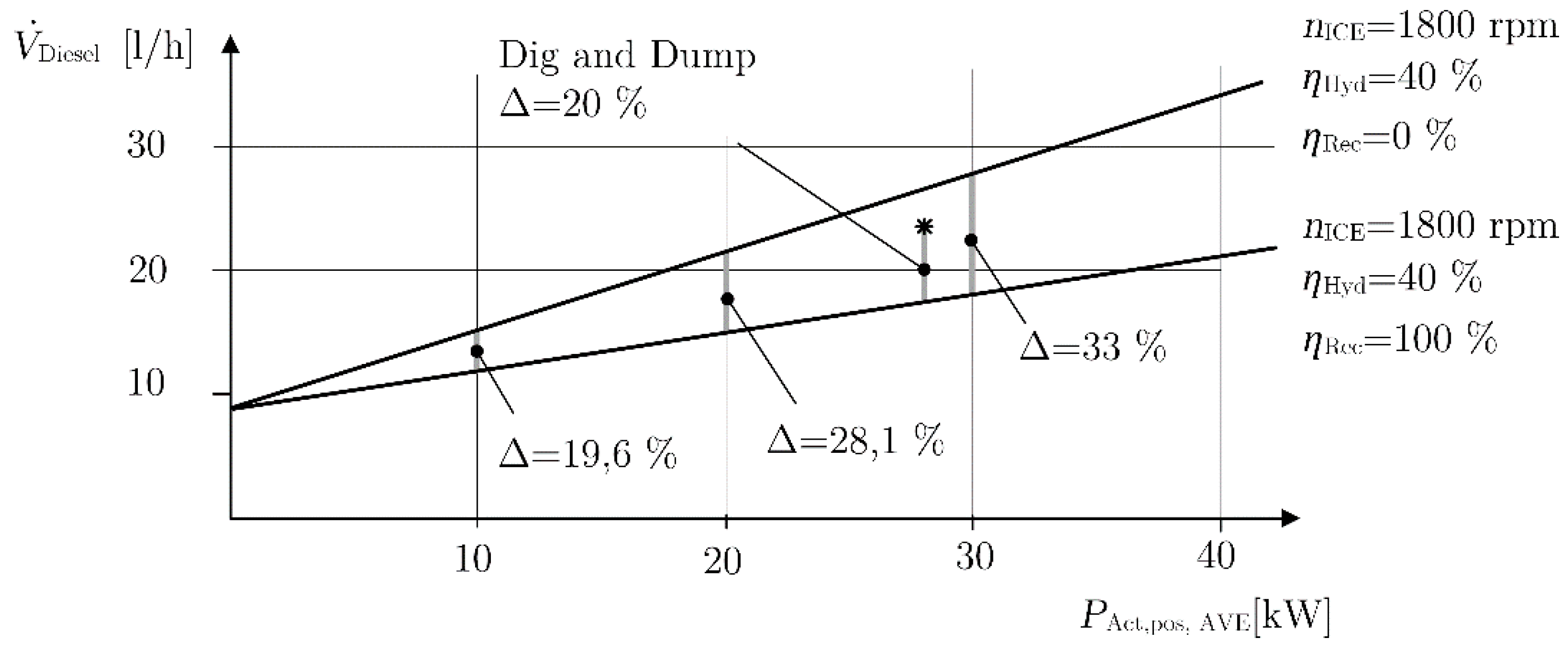
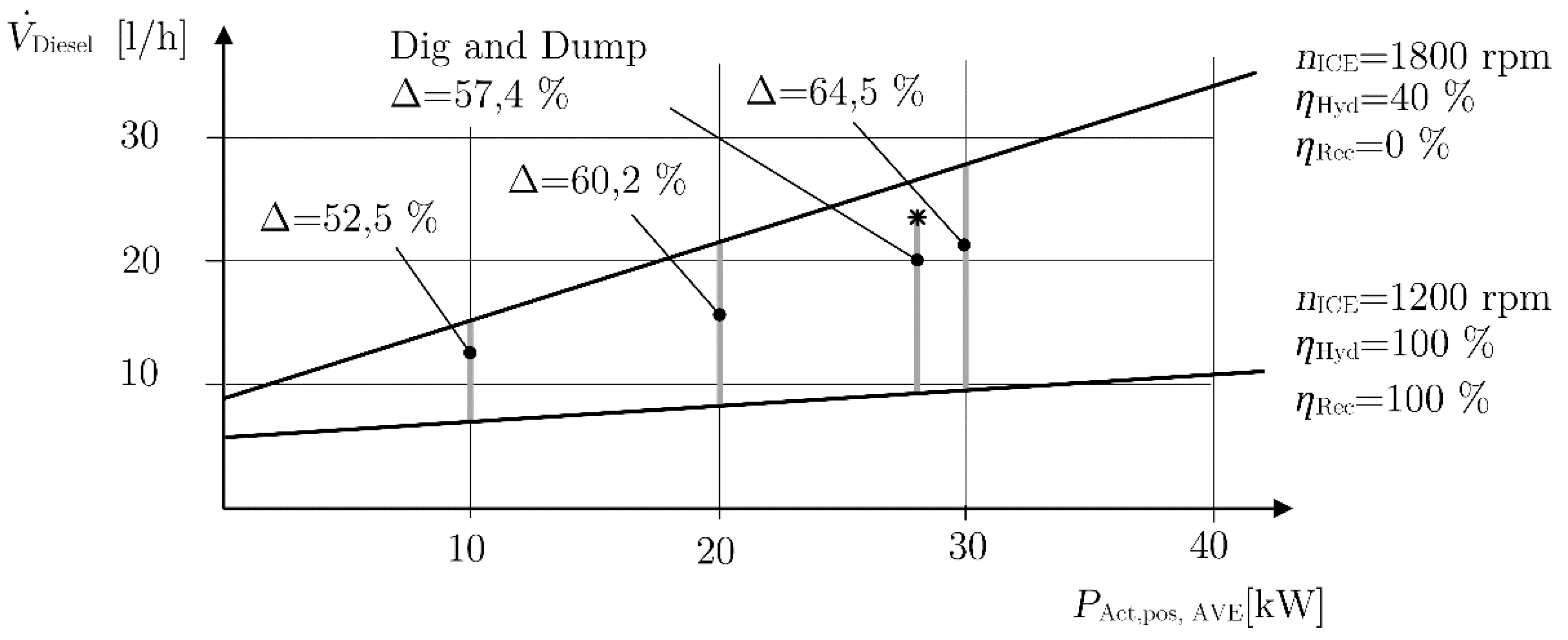
Firstly, the engines in most machines cannot even deliver the same amount of power as can be demanded by the pump. This may sound strange, but has to do with dimensioning. The pump size is selected to meet the maximum speed/flow rate requirements of all the actuators (implements + travel drive) when operating at the rated engine speed. System pressure is a function of the load and can reach values up to , but is typically around 200 bar. The pump’s corner power is, therefore, considerably greater than the power required during standard operation. Installing an engine with the same corner power capabilities as the pump in order to cover these infrequent cases would be expensive and require more space. As a result, it is quite common to find machines, in which the corner power of the pump is two or three times greater than the maximum engine power. Full actuator speed can only be maintained for average system pressures around 180 bar, thereafter a power limiting controller swivels the pump back preventing the engine from stalling.
Secondly, as the operator adjusts his joystick commands and the load changes, an actuator’s state can move through the load plane rather rapidly. Unfortunately, most engines cannot react so quickly to such rapid load changes and are prone to stalling. The pump controller and valves must assume this role, and ideally work in sync with the EECU, to ensure the dynamic power demand and supply are well matched. Achieving a well-tuned engine-pump interface is one of the major challenges in today’s mobile hydraulic systems [
19].
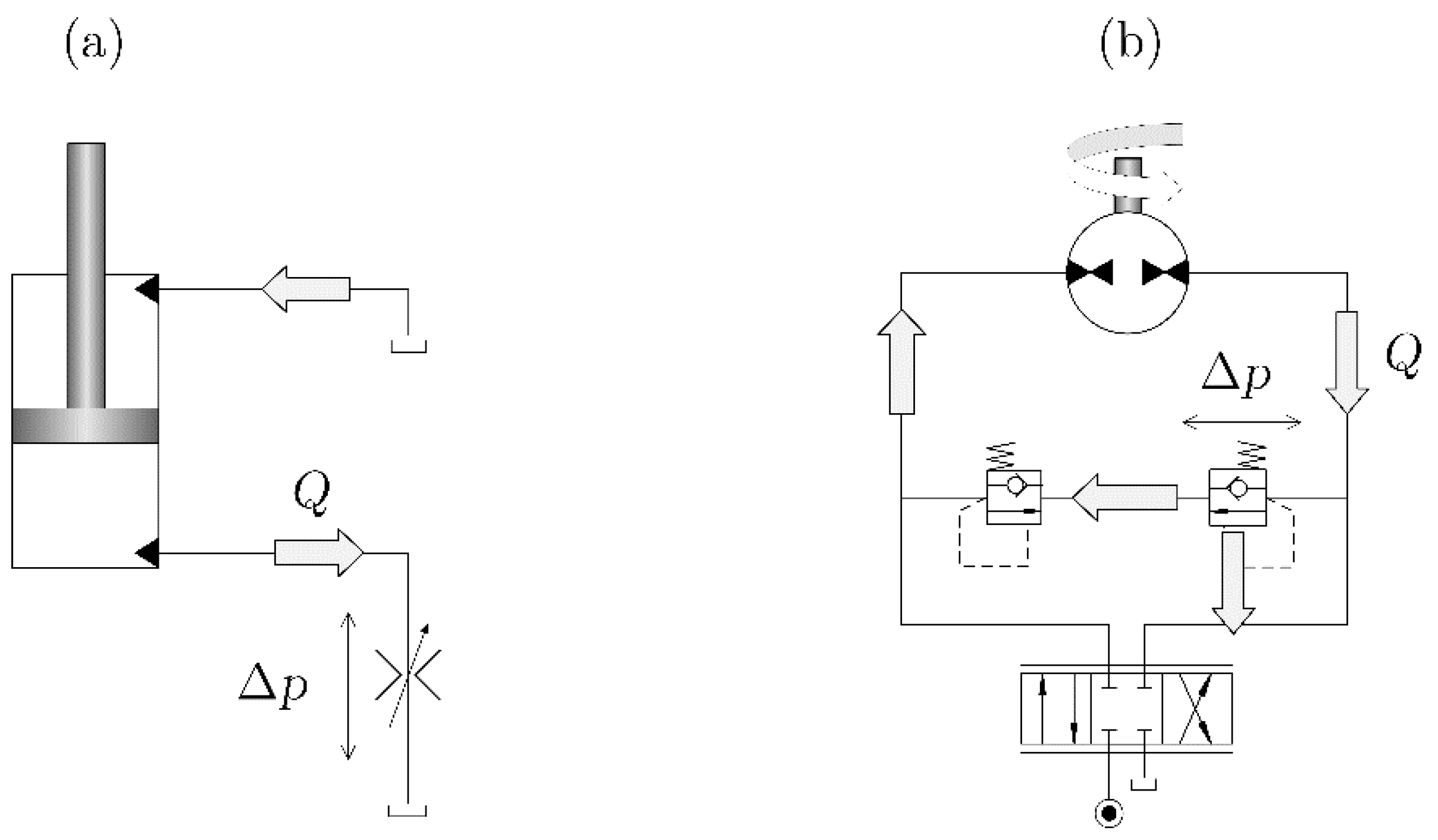
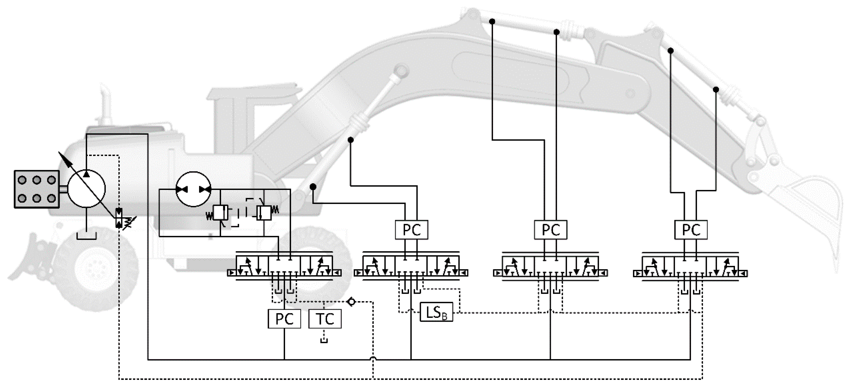
In contrast to most other mobile machines, excavators are capable of rotating their superstructure relative to the undercarriage by using the swing drive. The way in which the acceleration and deceleration of the swing is regulated largely determines the machine’s performance. Not only is this drive used approximately 60% of the time, it is also critical to safety because the operator’s field of vision changes as the machine turns. As a result, swing motion must be precise and have priority over other functions. Each OEM has its own specific solution, to attain the required swing motion without affecting the other actuators negatively. The single circuit flow sharing (SC-FS) system studied in this work, which also represents the most commonly used hydraulic system for wheeled excavators, is shown in
Figure 6.
The implement cylinders are controlled using downstream stream pressure compensated valves. Controlling the swing’s large inertia with such a flow controlled valve, causes high pressures during acceleration as the load pressure is primarily determined by inertial forces resulting from acceleration and not by external load forces from the environment [
20]. If the acceleration is not controlled appropriately, the system pressure can rise excessively leading to large pressure differences among the various actuators, which cause unnecessary throttling and forces the pump to swivel back thereby delivering less flow in order to avoid overloading the engine [
21]. Such issues are detrimental to performance. To overcome these issues, manufacturers have come up with various solutions.
Instead of regulating the flow rate to the swing, so-called torque control is used. In these circuits, the operator’s joystick command determines the maximum load sensing pressure of the swing drive and is used to directly regulate the swing torque and not the swing speed. To ensure the swing always receives exactly the flow it demands, regardless of the other actuator movements, an upstream pressure compensator with a lower spring pressure differential setting than the pump controller’s
is used [
22]. This gives the swing priority over the other actuators. This is an important safety function as the operator’s field of view changes during swing operation and unexpected obstacles may suddenly appear.
An additional feature of the circuit is the boom load sensing pressure bypass. During fast lifting operations, the load sensing line is directly connected to the boom piston side using a bypass throttle, causing the boom pressure to be the dominant pressure signal that is sent to the pump. This ensures that the swing pressure does not exceed the boom pressure, which results in minimal throttling and maximum pump flow, improving cycle times and efficiency [
20]. Some manufacturers also offer an energy efficient boom float function in which the boom down motion does not require any pump flow [
23]. These features represent the state of the art in today’s wheeled excavators.
To discuss the losses occurring within the hydraulic system, we must take a closer look at the pumps, valves and actuators.
2.2.1. Pump Losses
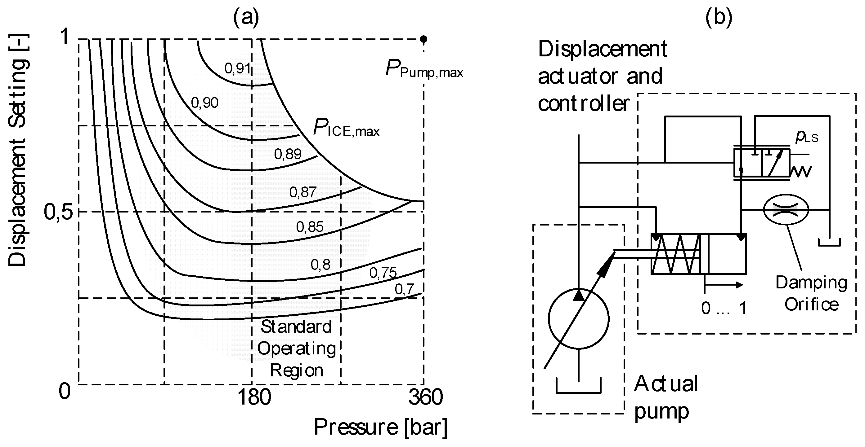
The hydraulic pump, almost exclusively of the axial piston type, is responsible for converting the mechanical output power from the engine into hydraulic power, in the form of flow and pressure. A typical pump efficiency map for a constant rotation speed is shown in
Figure 7a. Depending on the displacement setting and pressure, the efficiency can vary from as low as 60% to peak values of up to 91% at higher displacement settings and pressure levels [
24]. As with the engine, thinking in terms of efficiency can be misleading. The leakage and hydro-mechanical losses do not change depending on the displacement setting, they actually remain fairly constant. In reality, only the output power changes leading to a higher efficiency. A pump operating at a higher displacement actually consumes more energy as its power output is higher.
The mismatched corner powers of the engine and pump also create some additional effects. Pump operation in the upper right hand region is not even possible, meaning that the pump is forced to operate at lower displacement settings and efficiencies when system pressure is high. Studies have shown that depending on the cycle the pumps in a typical mobile hydraulic system are responsible for dissipating between 10% and 15% of the mechanical power supplied by the engine [
25,
26].
In the past couple of years, one further aspect concerning pump operation has become known. The values shown in typical pump efficiency maps are taken from measurements, in which the pump controller is inactive and the displacement actuator has been mechanically locked thereby not allowing the pump swash plate to vibrate. These are not realistic boundary conditions and do not represent how such units really operate in a machine. The pump’s controller is, in fact, constantly adjusting the swash plate and regulating the flow entering the system.
This causes two additional loss mechanisms. First, the hydro-mechanical controller usually has various damping orifices (
Figure 7b), which create additional leakage. The second loss mechanism is due to the dynamic high frequency oscillation of the swash plate [
27]. As the pump piston barrel rotates, a strong vibrating torque acts on the swash plate. In the case of tests, in which the swash plate is mechanically locked, this vibrating torque is counteracted by pump’s end stop. In reality, the pump controller must feed the swash plate with pressure in order to balance these torque oscillations, thereby increasing the energy consumed by the controller. Together these controller losses are by no means negligible and can decrease efficiency by up to ten percentage points [
27,
28].
Just like in a diesel engine, the concept of efficiency can be a bit misleading. A variable displacement pump operating in standby at near 0 displacement still consumes power. For example, a 210 cc pump operating at 1800 rpm and a standby pressure of 28 bar will consume around 4 kW of power. These parasitic losses increase with rotation speed and cannot be neglected as they increase the machine’s idle fuel consumption. A Willans representation of pump efficiency has yet to published, but would surely be extremely valuable.
2.2.2. Valve Losses
The flow leaving the pump(s) is distributed to the actuators using valves. The fundamental physics explaining the flow of fluid through a valve can be described using the orifice equation:
In order for a flow
Q to pass through a valve a certain pressure difference Δ
p, in other words a driving force, must be present. The amount of pressure needed depends on the valve’s geometry, described by the coefficient
, and spool position y. In summary, for a valve to function, part of the hydraulic power entering the valve must be dissipated as heat. These so-called pressure or throttling losses can be expressed as follows
In literature, there seems to be a number of misconceptions concerning throttling. Yes, due to their hydraulic resistance valves will always generate losses when supplying flow to an actuator, but if correctly sized, that is with a large enough value for , these losses can be kept low, down to only a couple of bar. The extreme throttling losses attributed to valves and so often cited in literature, are due to completely different reasons. These are worth mentioning.
The first and major cause is directly related to the nature of the hydraulic architecture. Multiple actuator systems, in which valves are used to distribute flow, delivered by a single pump are a classic example. Each actuator has its own independent pressure level, determined by the load it is currently subjected to. In order to deliver flow to each actuator the pump must supply the system with a pressure level greater than that of each actuator. Unfortunately, no matter how well the cylinder areas and kinematics are designed, there will always be instances, during which the individual actuator pressure levels are substantially different. This creates a complete mismatch between the pump pressure and actuator pressures. Unfortunately, valves can only operate according to the orifice equation and are not capable of performing a lossless transformation of the pump pressure down to a lower actuator pressure level. Consequently, the already existing pressure difference is used to generate the required flow, resulting in considerable losses, especially when the flow is large, see Equation (7).
Other than distributing flow, the valves must enable the operator to precisely regulate the movement of an actuator in all four load quadrants. This is done by regulating both the flow to the actuator using an inlet metering edge and the flow leaving the actuator using an outlet metering edge. The inlet edge is needed to control the actuator speed as it determines the amount of flow entering the actuator. The outlet edge, on the other hand, fulfils a different function. In quadrants II and IV, it is used as a type of brake and prevents runaway loads. In quadrants I and III, it is used to marginally throttle the flow leaving the actuator, thereby maintaining a pressure level of approximately 5 to 10 bar in the outlet chamber [
29]. This ensures that both the inlet and outlet chambers are always pressurized and act as springs, guaranteeing a higher natural frequency and better system response [
30]. For actuators undergoing four quadrant operation, finding an optimal outlet geometry involves compromise. The outlet resistance must be large enough to prevent the overrunning loads in quadrants II and IV, but preferably should not be too large to cause unnecessary throttling in the other two quadrants I and III.
In summary, it is important to differentiate between the following causes of throttling:
Throttling across the inlet edge in order to supply the actuator with flow
Throttling across the outlet edge to maintain controllability and prevent runaway loads
Throttling to equalise mismatched supply and actuator pressures


