1. Introduction
With the higher requirements of the economy and safety of the power grid, online condition-based maintenance (CBM) of power transformers without power outages is an inevitable trend for equipment maintenance mode [
1,
2]. The transformer CBM analysis relies on two basic groups: structured (e.g., numeric and categorical) and unstructured (e.g., natural language text narratives). Using structured data analysis, researchers have proposed a variety of transformer fault diagnosis algorithms such as the Bayesian method [
3,
4,
5], evidence reasoning method [
6], grey target theory method [
7], support vector machine (SVM) method [
8,
9,
10], artificial neural network method [
11,
12], extension theory method [
13], etc. These algorithms have achieved good results in engineering practice. However, for more unstructured data found in practice [
14,
15,
16,
17] (i.e., the malfunction inspection report), traditional artificial means of massive original document annotation and classification are not only time-consuming, but are also unable to achieve the desired results. For this reason, it has not been possible to adapt development of network information needs to the grid. Therefore, compared with structured data processing, it is more comprehensive for grid inspection personnel to effectively identify the massive unstructured text in the inspection malfunction report.
Deep learning achieved great success in speech recognition, natural language processing (NLP), machine vision, multimedia, and other fields in recent years. The most famous was the face recognition test set Labeled Faces in the Wild [
18], in which the final recognition rate of a non-deep learning algorithm was 96.33% [
19], whereas deep learning could reach 99.47% [
20].
Deep learning also consistently exhibits an advantage in regards to NLP. After Mikolov et al. [
21] presented language modeling using recurrent neural networks (RNNs) in 2010, he then proposed two novel model architectures (Continuous Bag-of-Words and Skip-gram) for computing continuous vector representations of words from very large data sets in 2013 [
22]. However, the model is not designed to capture the fine-grained sentence structure. When using the back-propagation algorithm to learn the model parameters, RNN needs to expand into the parameter-sharing multi-layer feed-forward neural network with the length of historical information corresponding to the number of layers to expand. Many layers not only make the training speed become very slow, but the most critical problem is also the disappearance of the gradient and the explosion of the gradient [
23,
24,
25].
Long short-term memory (LSTM) networks were developed in [
26] to address the difficulty of capturing long-term memory in RNNs. It has been successfully applied to speech recognition, which achieves state-of-the-art performance [
27,
28]. In text analysis, LSTM-RNN treats a sentence as a sequence of words with internal structures, i.e., word dependencies. Tai et al. [
29] introduce the Tree-LSTM, a generalization of LSTMs to tree-structured network topologies. Tree-LSTMs outperform all existing systems and strong LSTM baselines on two tasks: predicting the semantic relatedness of two sentences and sentiment classification. Li et al. [
30] explored an important step toward this generation task: training an LSTM auto-encoder to preserve and reconstruct multi-sentence paragraphs. They introduced an LSTM model that hierarchically builds a paragraph embedding from that of sentences and words, and then decodes this embedding to reconstruct the original paragraph. Chanen [
31] showed how to use ensembles of word2vec (word to vector) models to automatically find semantically similar terms within safety report corpora and how to use a combination of human expertise and these ensemble models to identify sets of similar terms with greater recall than either method alone. In Chanen’s paper, an unsupervised method was shown for comparing several word2vec models trained on the same data in order to estimate reasonable ranges of vector sizes to induce individual word2vec models. This method is based on measuring inter-model agreement on common word2vec similar terms [
31]. Palangi [
32] developed a model that addresses sentence embedding, a hot topic in current NLP research, using RNN with LSTM cells.
In the above papers, the RNN-LSTM is continuously improved and developed in the process of deep learning applied to NLP. At present, RNN-LSTM has many applications in NLP, but it has not been applied to the unstructured data in the grid. Unstructured data accounts for about 80% of power grid enterprises, which contain important information about the operation and management of the grid. In the malfunction inspection report, the unstructured data processing method is urgently needed to analyze the effective information.
The primary objective of this paper is to provide insight on how to apply the principles of deep learning via NLP to the unstructured data analysis in grids based on RNN-LSTM. The remaining parts in the paper are organized as follows. In
Section 2 and
Section 3, the description of the text data mining–oriented RNN and LSTM model are presented. In
Section 4, the malfunction inspection report analysis method based on RNN-LSTM is proposed. Experimental results are provided to demonstrate the proposed method in
Section 5. Conclusions are drawn in
Section 6.
3. Long Short-Term Memory Model
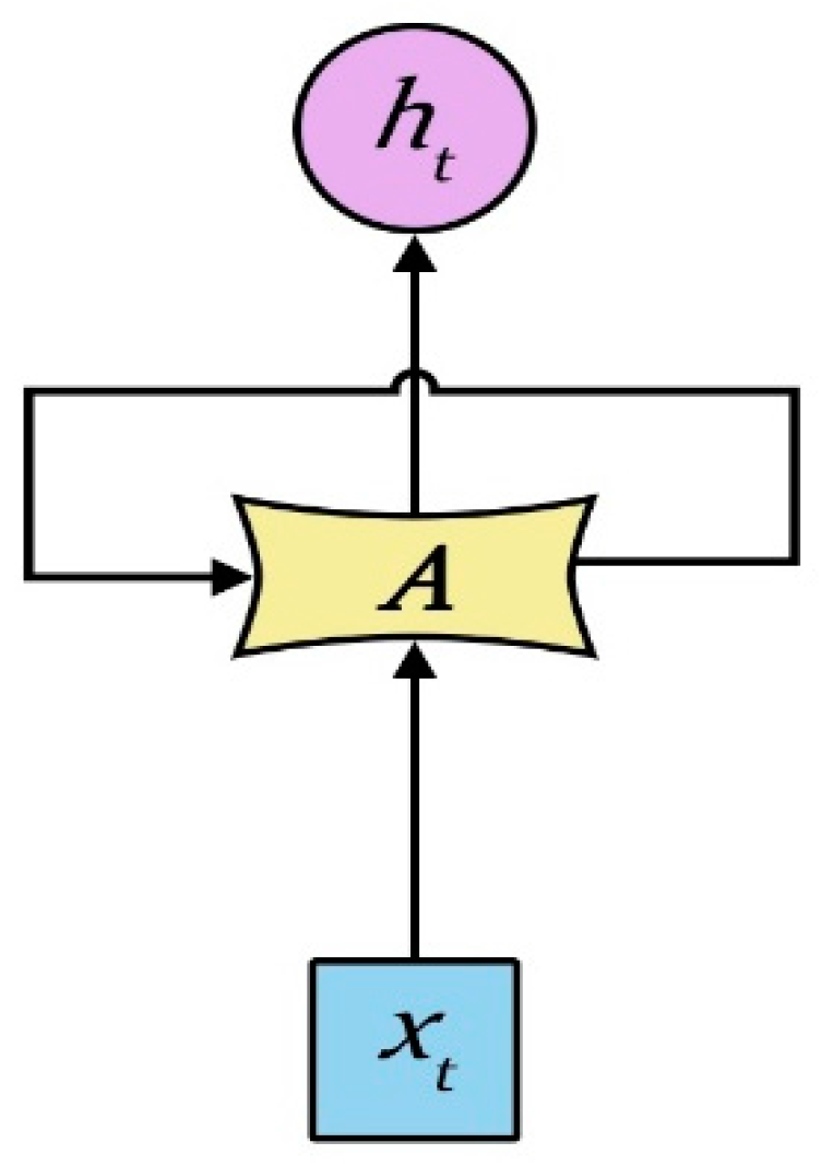
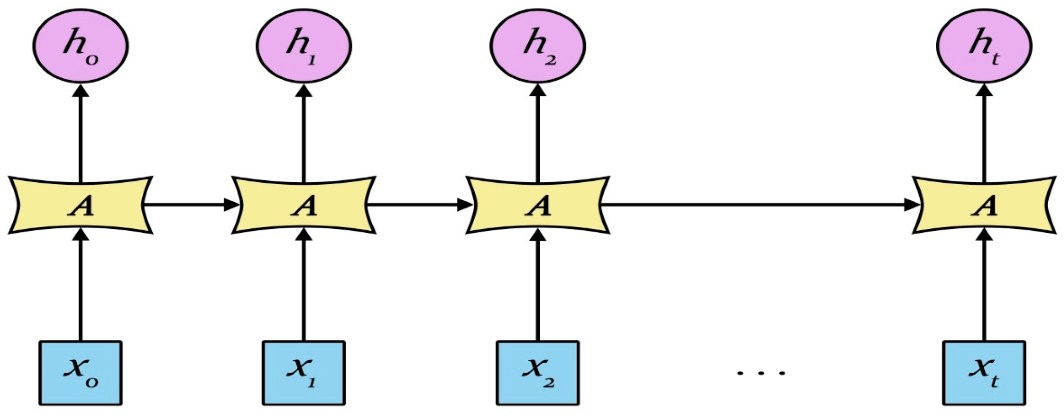
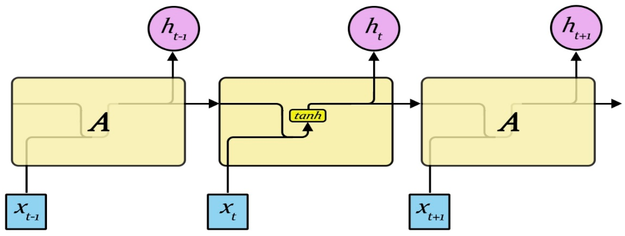
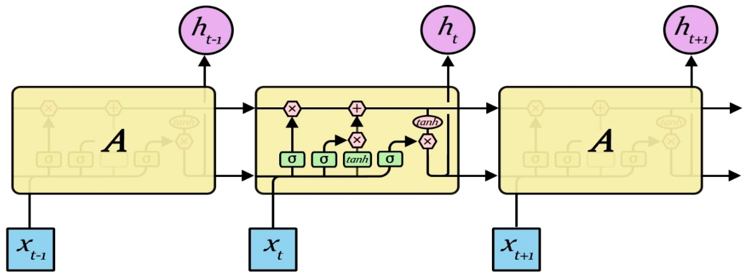
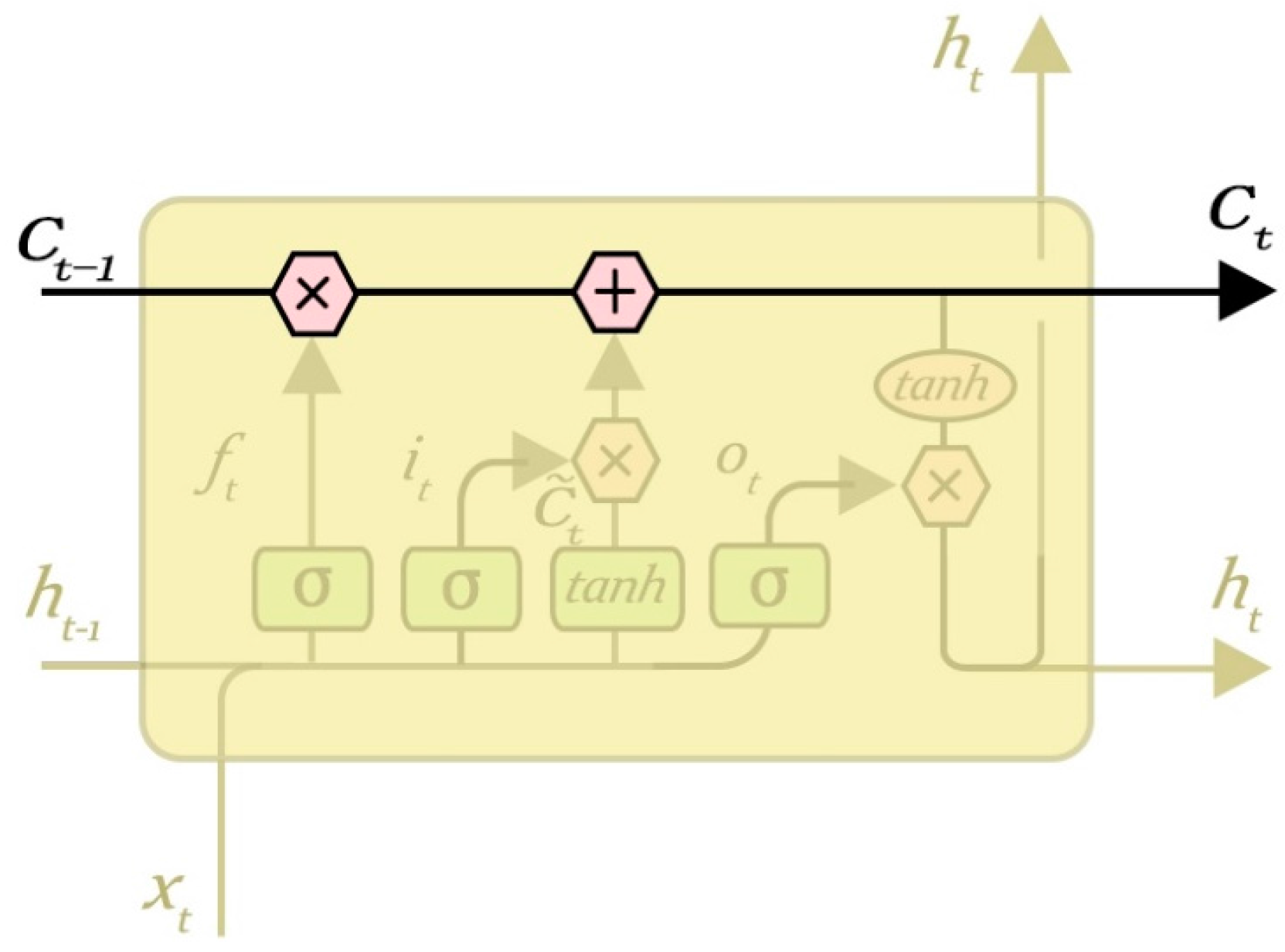
Although the RNN performs the transformation from the sentence to a vector in a principled manner, it is generally difficult to learn the long-term dependency within the sequence due to the vanishing gradients problem. The RNN has two limitations: first, the text analysis is in fact associated with the surrounding context, while the RNN only contacts the previous text, but not the following text; second, compared to the time step, RNN has more difficulties in the learning time correlation. A bidirectional LSTM (BLSTM) network can be used in the first problem, while the LSTM model can be used for the second. The RNN repeats the module as shown in
Figure 3, which only contains one neuron. The LSTM model is an improvement of the traditional RNN model; based on the RNN model, the cellular control mechanism is added to solve the long-term dependence problem of the RNN and the gradient explosion problem caused by the long sequence. The model can make the RNN model memorize long-term information by designing a special structure cell. In addition, through the design of three kinds of “gate” structures, the forget gate layer, the input gate layer, and the output gate layer, it can selectively increase and remove the information through the cell structure when controlling information through the cell. These three “gates” act on the cell to form the hidden layer of the LSTM, also known as the block. The LSTM repeat module is shown in
Figure 4, which contains four neurons.
3.1. Core Neuron
LSTM is used to control the transmission of information, it is usually expressed by
sigmoid function. The key to LSTMs is the cell state, the horizontal line running through the top of the diagram. The cell state is kind of like a conveyor belt. It runs straight down the entire chain, with only some minor linear interactions. It is very easy for information to just flow along it unchanged. The LSTM does have the ability to remove or add information to the cell state, carefully regulated by structures called gates. Gates are a way to optionally let information through. They are composed of a
sigmoid neural net layer and a pointwise multiplication operation. The state of the LSTM core neuron is shown in
Figure 5.
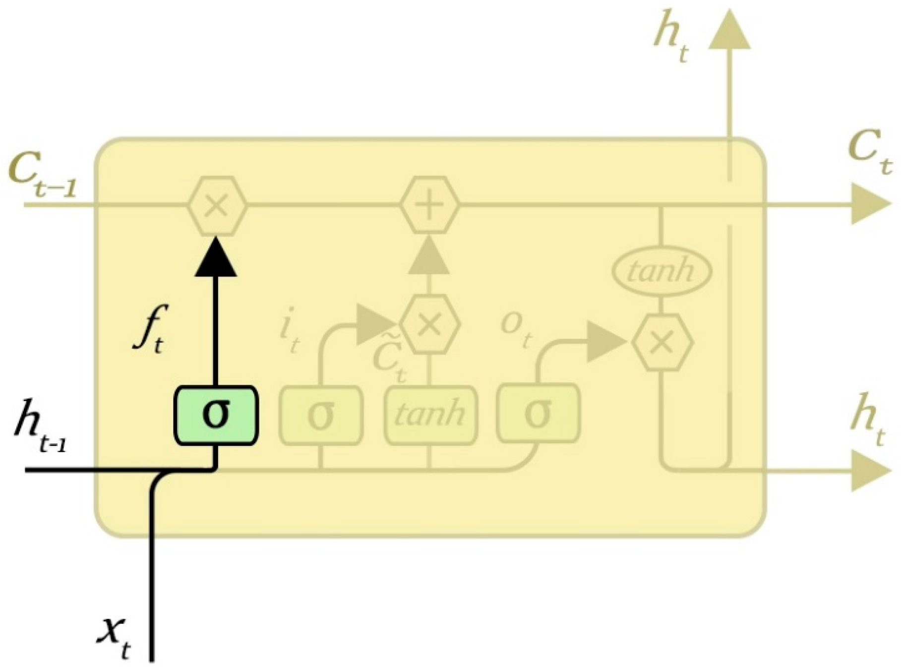
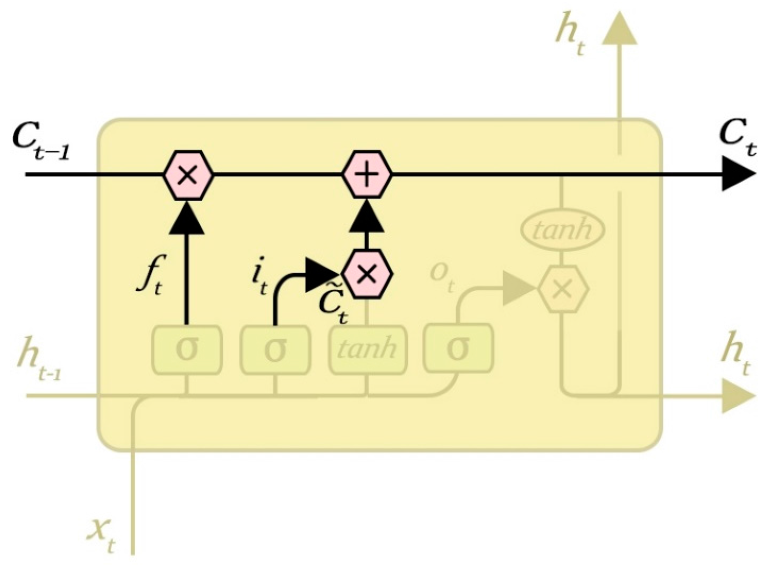
3.2. Forget Gate Layer
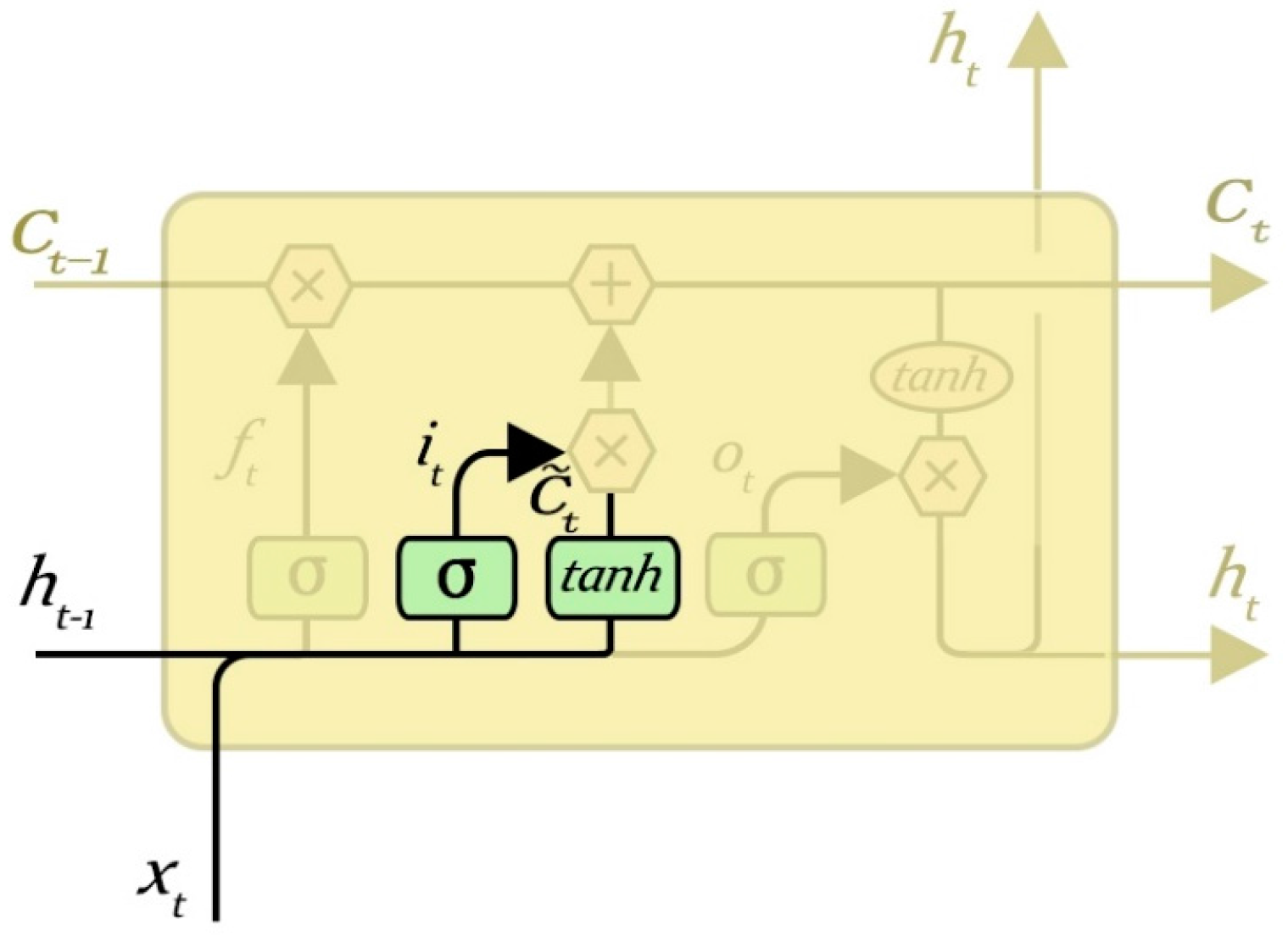
The role of the gate layer is to determine the upper layer of input information which may be discarded, and it is used to control the hidden layer nodes stored in the last moment of historical information. The forget gate computes a value between 0 and 1 according to the state of the hidden layer at the previous time and the input of the current time node, and acts on the state of the cell at the previous time to determine what information needs to be retained and discarded. The value “1” represents “completely keep”, while “0” represents “completely get rid of information”. The output of the hidden layer cell (historical information) can be selectively processed by the processing of the forget gate.
The forget gate layer is shown in
Figure 6, when the input is
and the output is
:
3.3. Input Gate Layer
The output gate layer is used to control the input of the cell state of the hidden gate layer. It can input the information through a number of operations to determine what needs to be retained to update the current cell state. First the input gate layer is established through a
sigmoid function to determine which information should be updated. The output of the input gate layer is a value between 0 and 1 of the
sigmoid output, and then it acts on the input information to determine whether to update the corresponding value of the cell state, where 1 indicates that the information is allowed to pass, and the corresponding value needs to be updated, and 0 indicates that it may not be allowed as the corresponding values do not need to be updated. It can be seen that the input gate layer can remove some unnecessary information. Then a
layer can be established by adding the candidate state of the neuron phase phasor, and the two jointly calculate the updated value. The input gate layer is shown in
Figure 7.
3.4. Update the State of Neurons
It is time to update the old cell state,
, into the new cell state
. The previous steps already decided what to do, and now we just need to actually do it. Multiply the old state by
, forgetting the information we decided to forget earlier; then add
. These are the new candidate values, scaled by how much we decided to update each state value. In the case of the language model, this is where we would actually drop the information about the old subject’s gender and add the new information, as we decided in the previous steps. The neurons’ state update process is shown in
Figure 8.
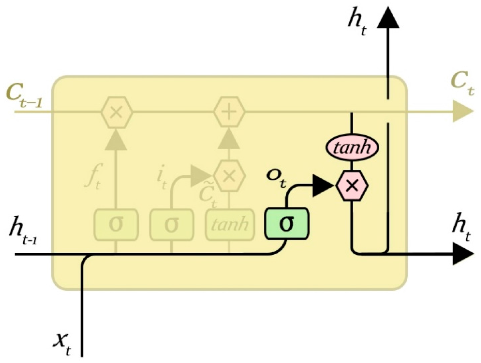
3.5. Output Gate Layer
The output gate layer is used to control the output of the current hidden layer node, and to determine whether to output to the next hidden layer or output layer. Through the output of the control, we can determine which information needs to be output. The value of its state is “0” or “1”. The value “1” represents a need to output, and “0” represents that it does not require output. Output control information on the current state of the cell for some sort of value can be found after the final output value.
Determine the output of the neurons as (6) and (7), and the output gate layer is shown in
Figure 9.
4. Malfunction Inspection Report Analysis Method Based on RNN-LSTM
To learn a good semantic representation of the input sentence, our objective is to make the embedding vectors for sentences of similar meanings as close as possible, and to make sentences of different meanings as far apart as possible. This is challenging in practice since it is hard to collect a large amount of manually labeled data that give the semantic similarity signal between different sentences. Nevertheless, a widely used commercial web search engine is able to log massive amounts of data with some limited user feedback signals. For example, given a particular query, the click-through information about the user-clicked document among many candidates is usually recorded and can be used as a weak (binary) supervision signal to indicate the semantic similarity between two sentences (on the query side and the document side). We try to explain how to leverage such a weak supervision signal to learn a sentence embedding vector that achieves the aforementioned training objective. The above objective to make sentences with similar meaning as close as possible is similar to machine translation tasks where two sentences belong to two different languages with similar meanings, and we want to make their semantic representation as close as possible.
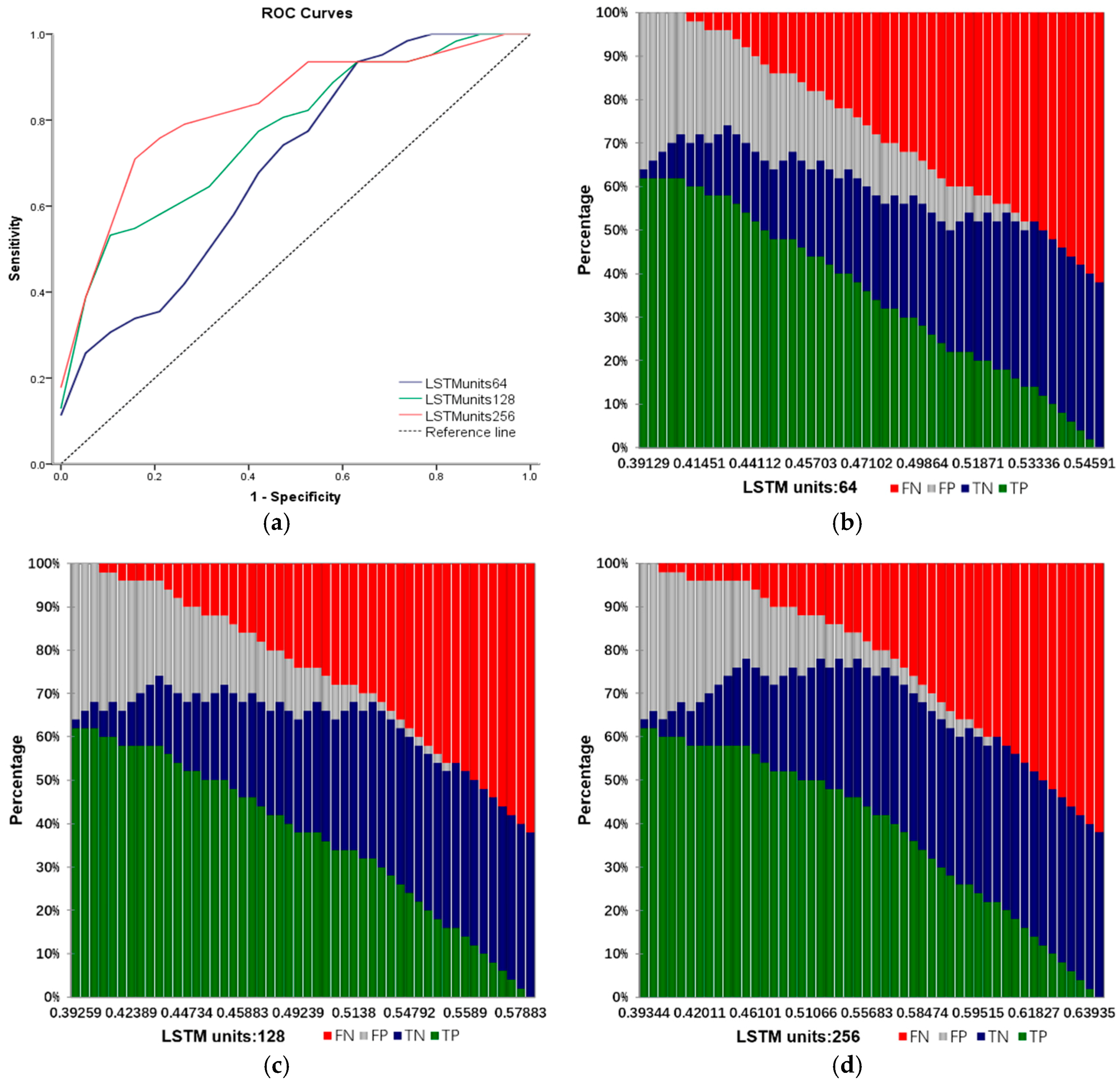
In this paper, the algorithm, parameter setting and experimental environment are introduced as follows:
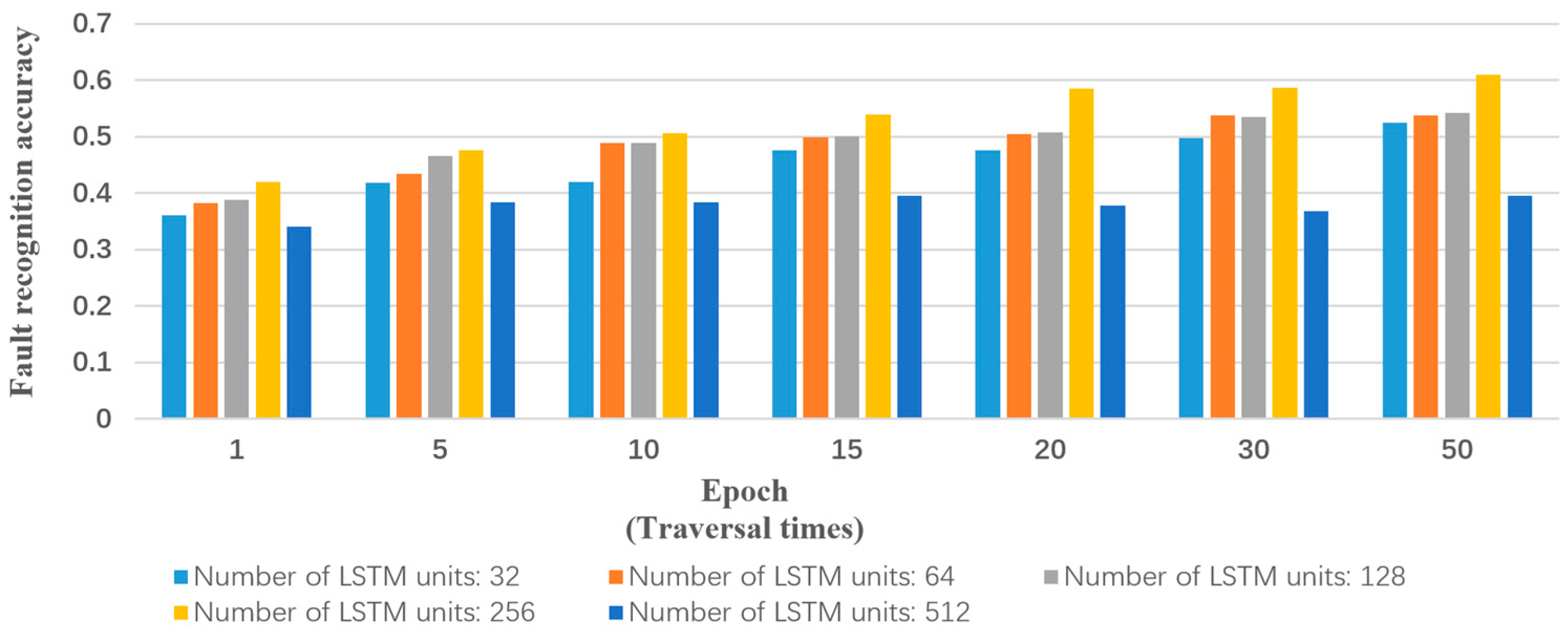
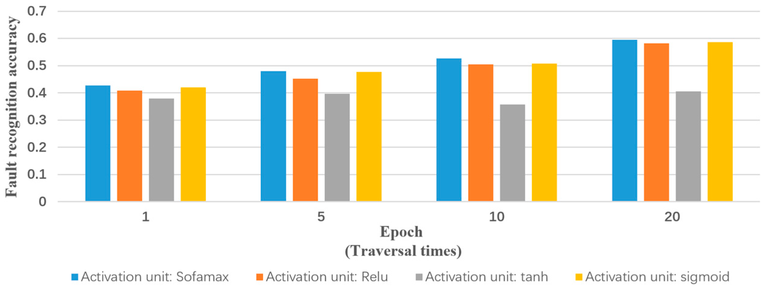
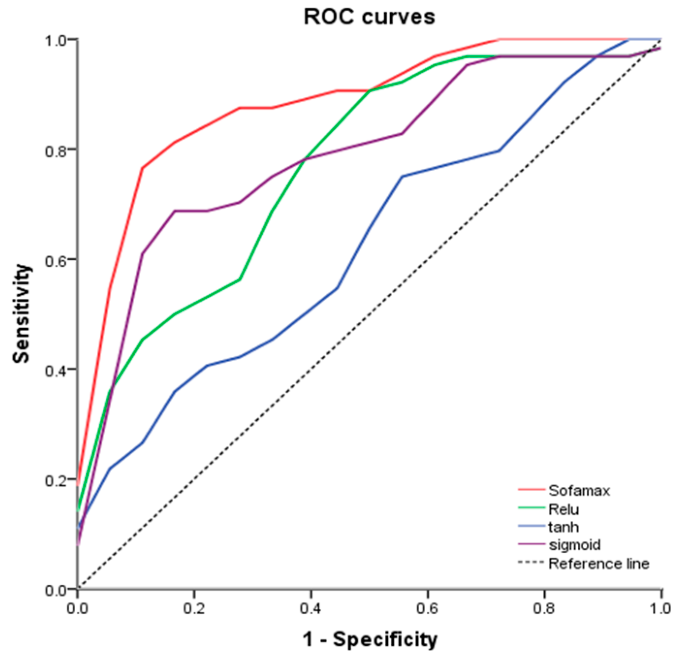
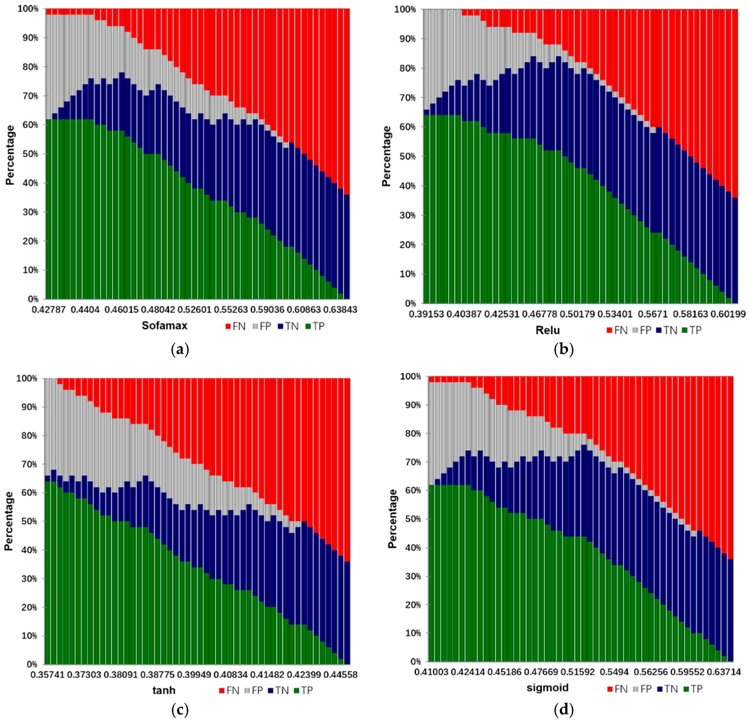
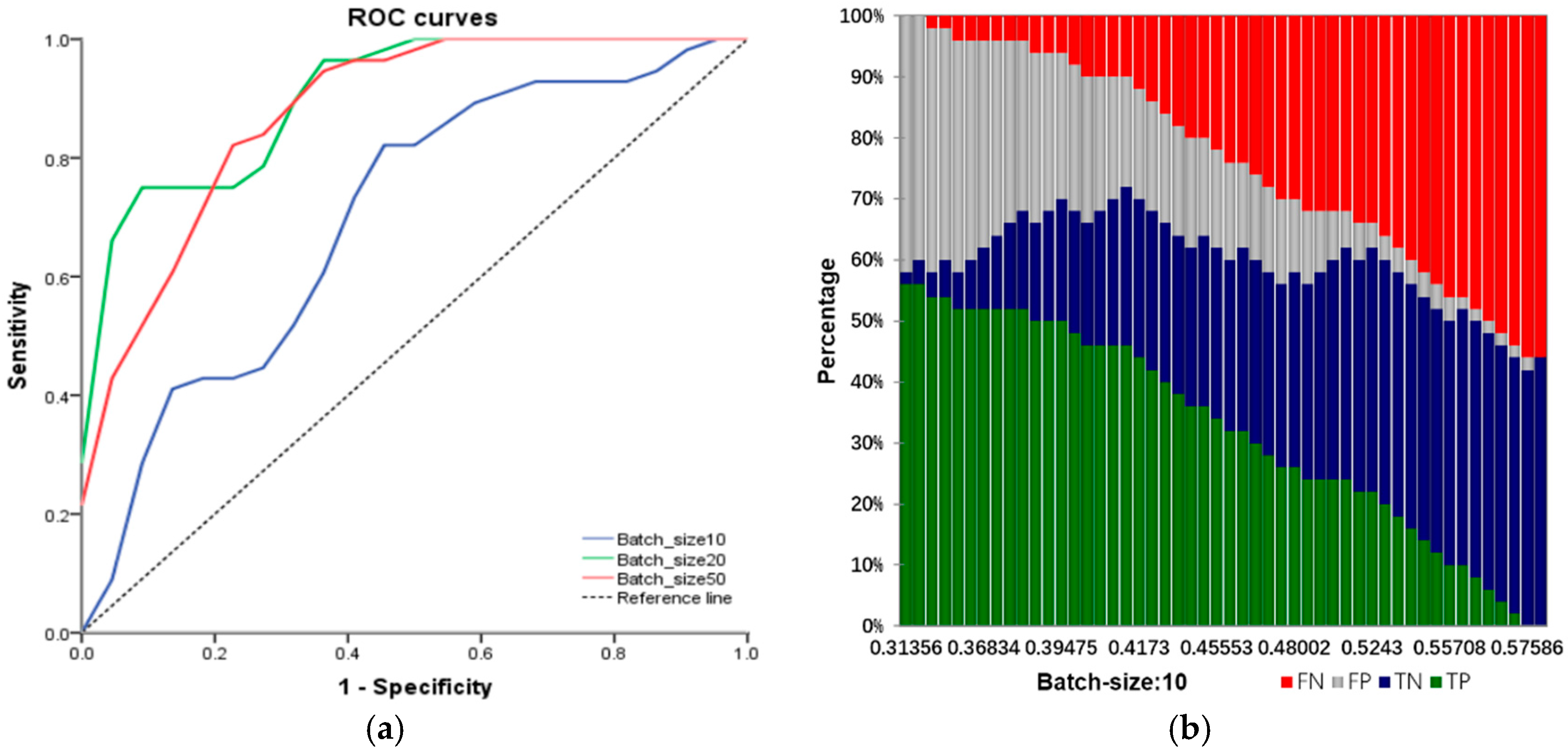
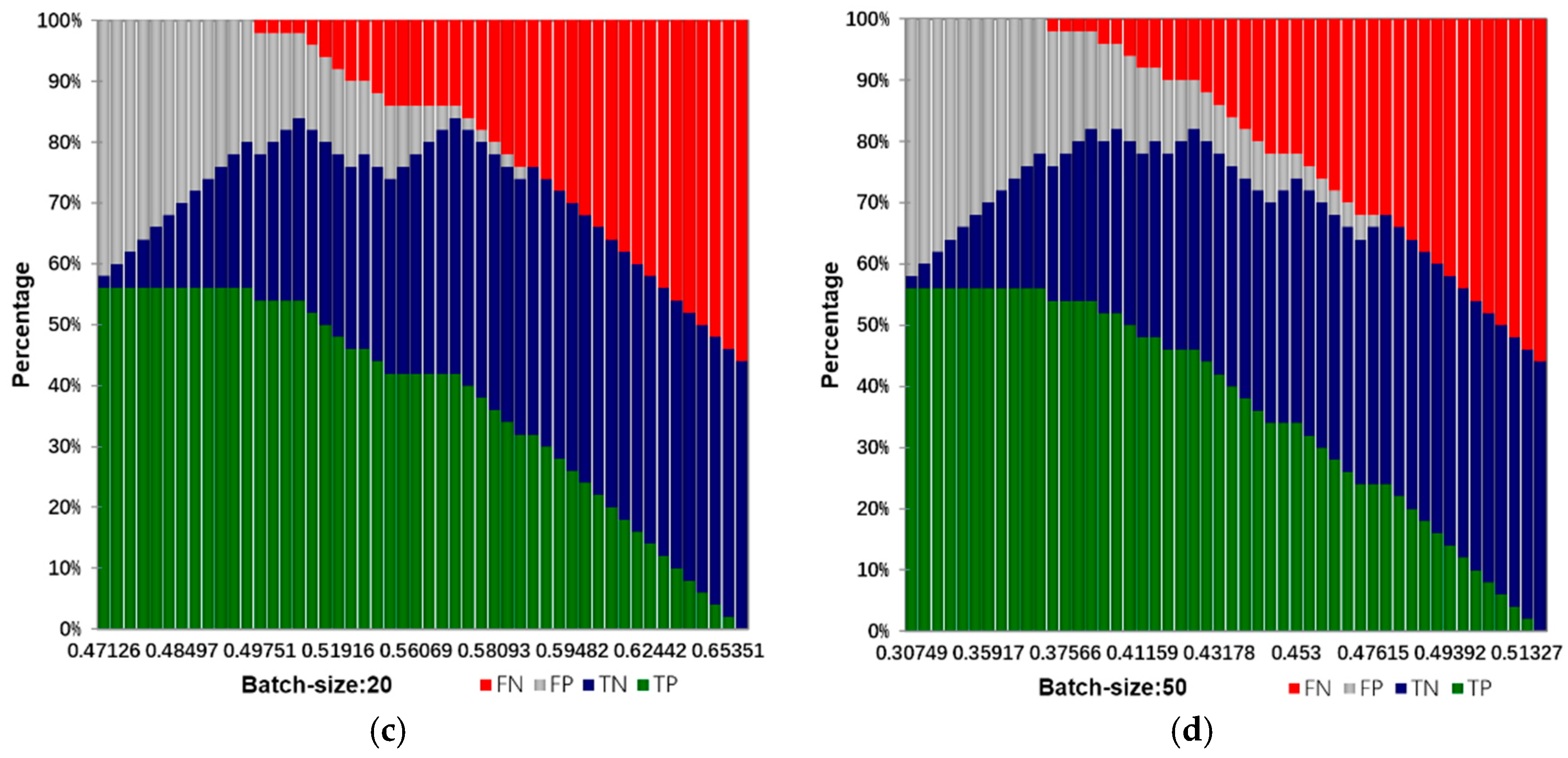
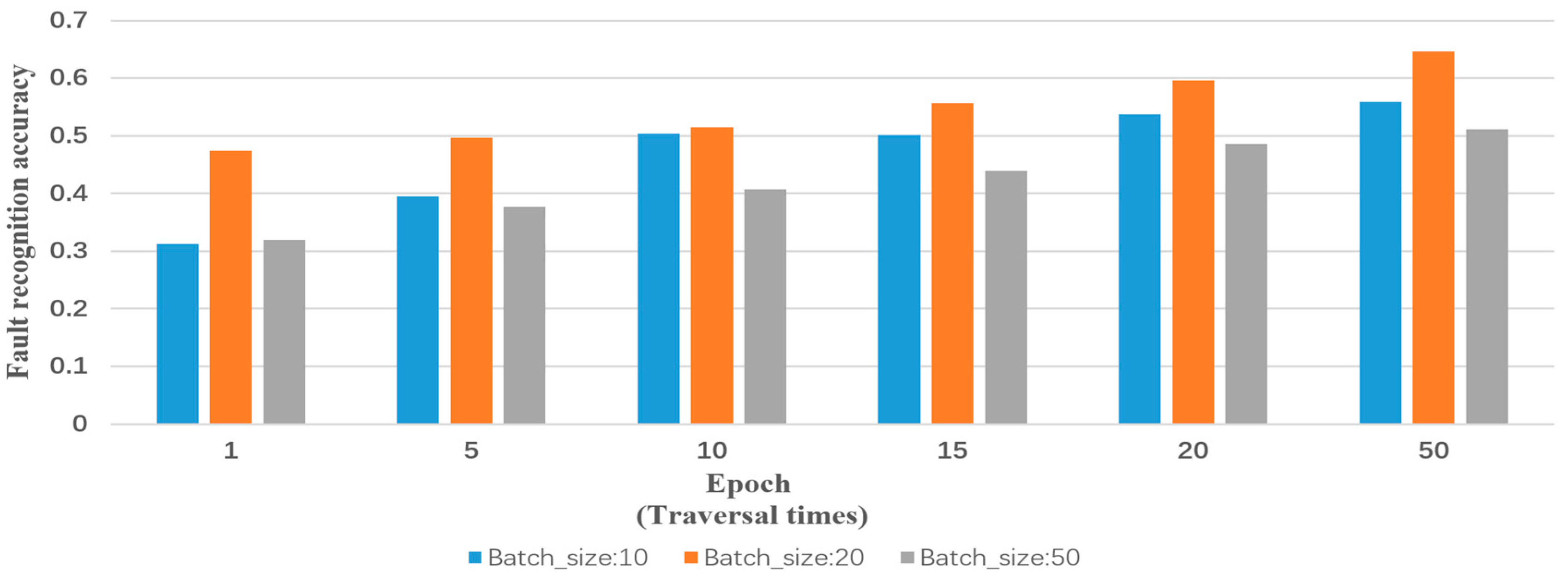
Input: training samples and test sample (including various types of reports and their labels). The number of truncated words: maxlen = 200. Minimum number of words: min_count = 5. The parameters of the model: Dropout = 0.5, Dense = 1. Activation function type: Sofamax, Relu, tanh and sigmoid. Number of LSTM units: 32; 64; 128; 259; 512. Output: classification results and fault recognition accuracy of test samples. Initialization: set all parameters of the model to small random numbers.
Experimental operating environment: operating system: Windows 10; RAM: 32 G; CPU: XeonE5 8-core; graphics: NVIDIA 980M; program computing environment: Theano and Keras.
The process of the training method for RNN-LSTM is presented in
Appendix B.


