Optimal Design of a Multi-Carrier Microgrid (MCMG) Considering Net Zero Emission


1
Department of Electrical Engineering, Faculty of Electrical Engineering, Science and Research Branch, Islamic Azad University, Tehran 14778-93855, Iran
2
Department of Electrical Engineering, Faculty of Electrical Engineering, Iran University of Science and Technology, Tehran 16846-13114, Iran
3
Department of Electrical Engineering, Faculty of Electrical Engineering, Sharif University of Science and Technology, Tehran 11365-11155, Iran
*
Author to whom correspondence should be addressed.
Energies 2017, 10(12), 2109; https://doi.org/10.3390/en10122109
Submission received: 15 August 2017
/
Revised: 6 November 2017
/
Accepted: 9 November 2017
/
Published: 12 December 2017
Abstract
:In this paper, a two-stage optimum planning and design method for a multi-carrier microgrid (MCMG) is presented in the targeted operation period considering energy purchasing and the component’s maintenance costs. An MCMG is most likely owned by a community or small group of public and private sectors comprising loads and distributed energy resources (DERs) with the ability of self-supply to regulate the flows of various energies to local consumers. The operation cost is undoubtedly reduced by selecting the proper components. In the proposed model, the investment and operation and maintenance costs of MCMG are simultaneously carried out in order to choose the right component and its size in the given period. Moreover, in this innovative model, net zero emission (NZE) is regarded as an environmental constraint. The genetic algorithm of MATLAB and the mixed-integer nonlinear programming (MINLP) technique of GAMS (general algebraic modeling system) software are used to solve the optimization problem. Illustrative examples show the efficiency of the proposed model.
1. Introduction
Currently, various energy infrastructures (for example, electricity, natural gas, and local district heating systems) are operated and designed individually. Most research has thus far focused on the operational or structural optimization of the microgrid (MG) and its infrastructures independently [1]. A few recent publications have, however, shown interest in the operation and planning of multi-carrier energy systems simultaneously, instead of focusing on a single carrier [2,3,4,5,6,7,8].
A microgrid (MG) which includes several energy carriers is called a multi-carrier microgrid (MCMG). The main challenge in the operation of the MCMG is the optimal usage of different energy resources and equipment. In previous studies, the operation and planning of different energy infrastructures, such as electricity, natural gas, heat, etc. were separately studied; this caused a restriction in optimal operation. The higher penetration of small scale energy resources (SSERs) with gas consumption, especially co- and tri-generation, has, however, increased the enthusiasm for the usage of network services among energy carriers [9]. For this purpose, integrated multi-carrier energy systems have been discussed in certain works of scientific literature [10,11]. The concept of the energy hub (EH) system was introduced in order to define the multi carrier-system and examine the various energy-form impact on each other infrastructure as well [10].
Energy hub systems comprise a variety of energy carriers, converters, and storages to meet demands [12]. This model of the system has been investigated from the standpoint of operation [13,14] and planning [15]. In fact, the main idea of MCMG is to couple the different carriers using current energy infrastructures in a limited geographical district while various load requirements are satisfied [16]. Certain examples of real facilities that can be modeled as a MCMG include the supply of industrial plants (steel work, paper mills), big building complexes (airports, shopping malls, and hospitals), and rural and urban districts. The co- and tri-generations, particularly combined heat and power (CHP), plays a substantial role in these multi carrier energy (MCE) systems [17]. The work in [18] proposes three energy dispatch algorithms to minimize the total operational cost of a residential combined heat, cooling and power unit. The results indicated that hybrid dispatch algorithm is the financially state in comparison with thermal or cooling dispatches.
Integrating and coupling different energy carriers and sources in an MCMG has a number of potential advantages over a single carrier microgrid, such as reliability improvement, enhancement of the energy management system’s performance to supply demands, synergy enhancement, and operation cost reduction [15]. In consequence, a comprehensive analysis for the optimal coordination of the various energy systems is indispensable for short-term operations and the long-term planning of energy sources [19]. It is observable that the proper planning of components guarantees an efficient and optimal operation of MCMG [20]. An expansion planning of an energy system would determine the optimal size, location, and time for the installation of equipment over a planning horizon according to its constrains and requirements [16]. This problem of the basis of its planning horizon is classified into static, quasi-dynamic, and dynamic planning [19,21]. It is apparent that a dynamic planning solution can be more optimal and realistic in comparison to static planning.
Traditional sources and component design in an MCE system have often focused on one energy form without taking into account its interactions with other types of energies. In any case, the issue is whether the separated planning of energies and cogenerated components without considering the synergies among various forms of energy in an MCMG would be adequate for the effective optimal planning of interdependent energy infrastructures [22]. Hence, the interactions of multiple carriers are increased by the co-optimization planning of multiple-energy infrastructures.
The long-term planning and short-term operation of equipment are the main concerns in the MCMG. The different operational issues in the MCMG, such as economic dispatch [23,24], optimal power flow [7,13,25], unit commitment [26,27], and the optimal integration of the various energy carriers [8,28], are primarily discussed. These topics are discussed from different point of views as shown below. An efficient control algorithm to integrate, manage and control various sources in a microgrid is precisely modeled [29]. The proposed model forecasted the generation of renewable sources and estimated the state of charges in batteries to invoke the appropriate mode of operation for achieving an economic operation. Furthermore, faster communication topologies have been deployed to achieve a better response time for the control commands at local as well as centralized controllers. The prior researches are focused on AC microgrid operation and planning, whereas DC or hybrid microgrids are not addressed. A probabilistic model for a day-ahead optimal operation of a hybrid microgrid system is presented in order to fulfill the required load demand [30]. The modeling goals in this paper are the minimization of microgrid operation costs as well as maintenance and greenhouse gas emissions costs. Furthermore, the adjustment of uncertain parameters inside the approach is acquired by utilizing the Monte Carlo simulation. In [31], the expansion planning of electric and natural gas transmission systems is proposed in a market-based environment. On the other hand, the optimal sizing of components such as CHP and the combined cooling, heating, and power (CCHP) unit as the primary components of the MCE system inside an MCMG are investigated in [32,33], respectively. The optimal selection and the sizing of components inside an MCE system are regarded from different objective functions such as costs, efficiencies, and costs and benefits. In [34,35] the reliability indices of multi-carrier system planning are considered.
Optimal supplying of loads in an MCE system depends not only on the proper operation of equipment but also on system design. The simultaneous operation and planning of the MCE system is, therefore, required [1,8]. In order to find the optimal size of CHP and CCHP, a united optimization problem of planning and operation strategy is presented in [36,37,38]. Furthermore, operation and planning is carried out simultaneously in an EH system along with reliability constraints [16]. The work in [39] analyzes a framework to determine the optimal design of three interconnected energy hubs under uncertainty of energy price market. The objective of this paper is to evaluate and minimize the total net present value (NPV) cost, including investment, operation, energy interruption and CO2 emission costs. It is shown that the availability of district heating system leads to less cost installation cost because the installation of heat storage, boiler and absorption chiller is avoided.
The increase in global temperature is significantly changing our planet’s climate, resulting in more extreme and unpredictable weather [40]. On the other hand, fossil fuel-based CO2 emissions are a limiting constraint for the usage of fossil fuels on a long term basis [41,42]. Lately, a new definition, net zero emission (NZE), has been introduced to reduce pollution all over the world. The definition of net zero energy and net zero emission buildings (nZEB) are described and distinguished in [43]. The effect of the additional cost of CO2 emissions on the network cost is considered in [44]. The most competitive and least-cost solution for achieving a NZE energy system is through the usage of renewable energy resources (RERs) [45]. In fact, to reach the goal of NZEs, fossil fuel-based energy demand should be mainly replaced by RERs. In [46], the impact of designing the photovoltaic (PV) system on the greenhouse gas (GHG) emission balance in a nZEB is analyzed. Moreover, the assessment and influence of the PV system design on the embodied and avoided emissions are objected in order to minimize the environmental emissions.
The prior work on MG design reveals that the optimal design and planning of a multi-carrier microgrid (MCMG), developed by transformer, CHP, boiler, PV panels, pre-established energy storage systems (ESSs) and elastic loads considering NZE constraint have not been investigated. Therefore, this paper presents a two-stage optimum static planning method for an MCMG including the selection and optimal sizing of the existing components. The investment and installation costs over the planning horizon in addition to the operation costs (maintenance and fuel prices) at a given period are calculated in terms of the net present value (NPV) factor. Furthermore, NZE is regarded as an environmental constraint, and the chronological electrical and heat load curves for each year are distinguished as two typical days and two different months—one day for weekdays and one day for weekends. Since the load is classified into controllable/non-controllable, therefore, the effectiveness of the existing controllable loads in MCMG planning with a novel approach of the demand response (DR) program is investigated. The proposed time-based DR program correlates the final energy price of responsive loads for multiple carriers with energy market price, energy purchase, and on-site generations. The optimization problem is solved by a compound method that combines the genetic algorithm of MATLAB and the mixed-integer nonlinear programming (MINLP) of the GAMS software, which. The main contributions and innovation of this paper are as follows:
- Modeling the cooperative operation and planning the proposed MCMG in a two-stage model in the presence of responsive loads.
- Considering the NZE balance as an environmental issue.
- Using a compound method to solve the co-optimization problem.
The remaining sections of this research are organized as follows: Section 2 introduces the description of the problem; Section 3 and Section 4 presents the mathematical modeling and describes the solution method; the simulation and the numerical results are illustrated and discussed in Section 5; and a brief review of the research is included in Section 6.
2. Problem Description
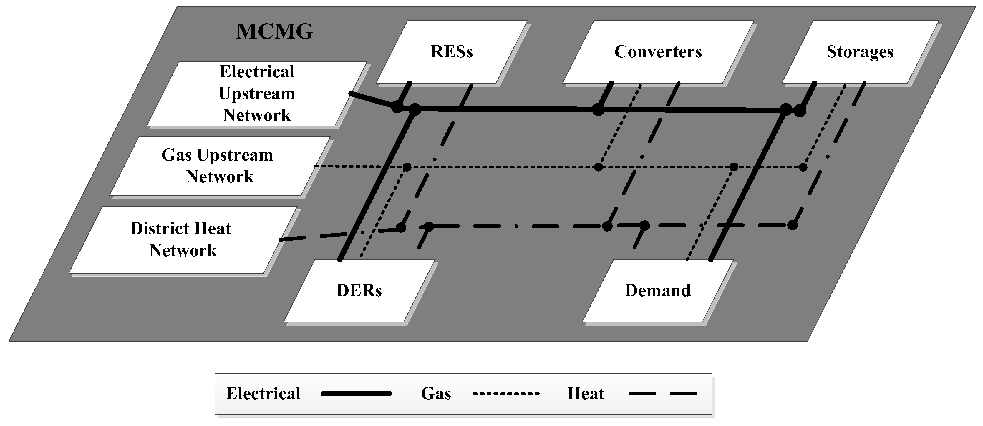
Microgrids, which comprise various energy carriers, are known as multi-carrier microgrids (MCMGs) as shown in Figure 1. The optimal supply of various loads in an MCMG depends not only on the proper operation of components, but also on the structure of these systems. In order to have a significant cost reduction while demands are satisfied, the MCMG design along with its operation needs, therefore, has to be executed.
2.1. Sampled MCMG
A multi-carrier microgrid is formed of a low- or medium-voltage electrical network alongside networks of other energy carriers, including natural gas and heat. In this case, energy conversion is possible through energy converters. Besides the converters, the distributed energy resources (DERs), such as energy storage elements and RERs, can satisfy the demand and bring about a significant reduction in the energy cost with regard to time of use (TOU) carrier’s prices. The demand side management program can provide more flexibility to the network for meeting the demand at any given period. In this paper, an MCMG with coordination among its components to fulfill multiple energy demands for 24 h is modeled for the test case of the MCMG structure as depicted in Figure 2.
2.2. MCMG Design
The expansion-planning problem determines the optimal type and capacity, location and time for the installation of each component in case the loads are optimally satisfied. In order to find and assess the proper size and type of available components inside an MCMG as shown in Figure 3, therefore, it is required to draw a realistic model and an optimal solution. In this paper, an MCMG in a single bus mode is drawn for the planning problem, in which the availability of a transformer, CHP, boiler, and PV are considered ideal. In addition, electrical and thermal storages with specified capacities are located inside the proposed MCMG. The main aim is to select the best components in a static planning.
2.3. Net Zero Emission Definition in the MCMG Network
In the coming decades, based on the COP21 (21st Conference of Parties) Paris agreement, certain countries are obliged to reach a NZE system by 2050 [44,47]. Energy production is, by far, the largest source of GHG emissions. This means that fossil-fuel consumption needs to be completely banned in these countries, particularly because growing forests are limited to eliminate a significant chunk of emissions, and carbon capture and storage technology is very expensive to be utilized.
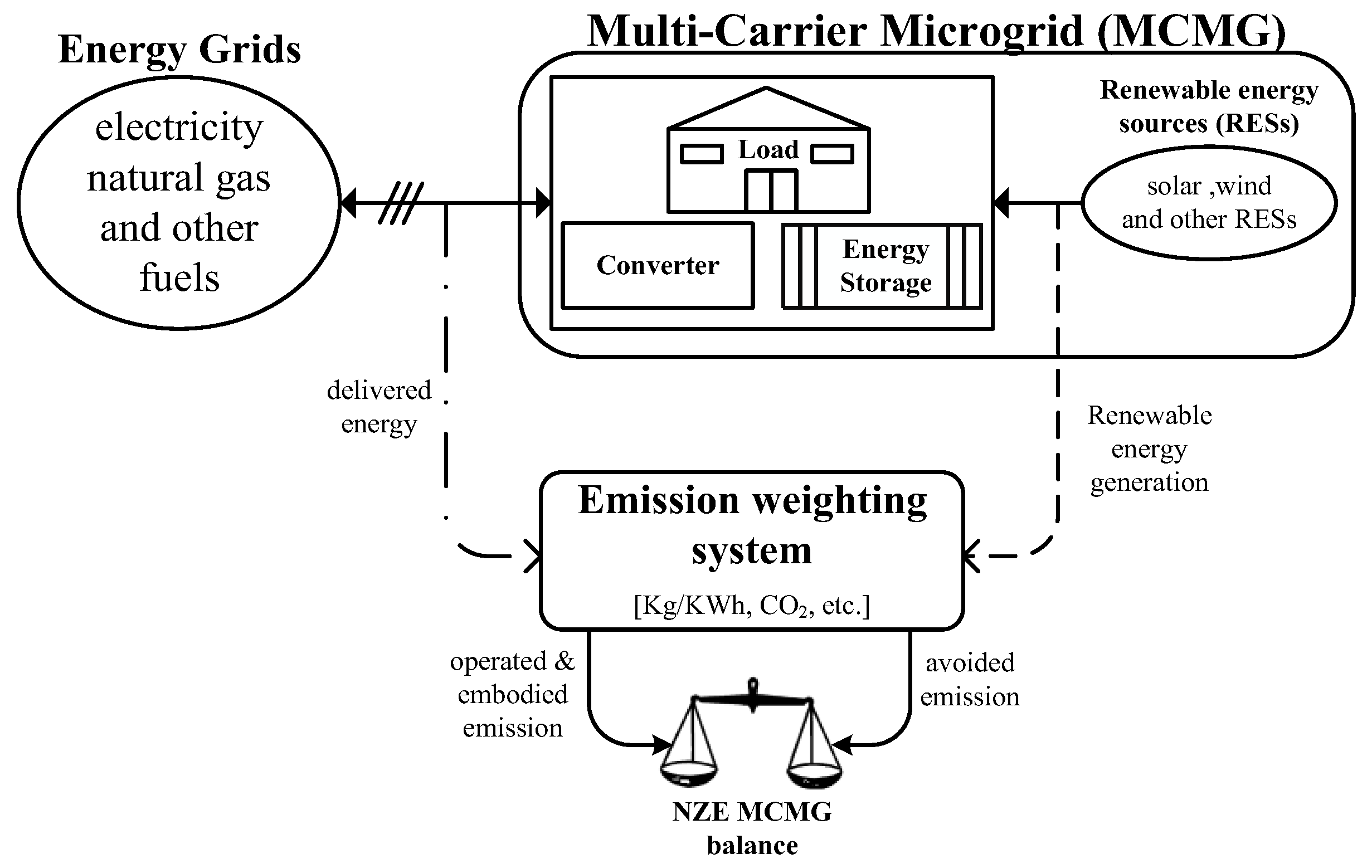
In a NZE system, the emissions associated with the amount of received energy to operate the system (operational emissions) and the energy used to produce the system materials (embodied emissions) are offset by on-site renewable generations (avoided emissions). The main strength of this idea is the weighting system that keeps the NZE balance in the system. The word “net” indicates that the avoided and embodied emissions, which are calculated by multiplying an emission factor of energy export and import to/from the system, have to be balanced over a specific period of time (usually a year) [48]. The only way to reach NZE balance and reduce GHG emissions is to replace fossil fuel-based units by renewable energy counterparts to fulfill the demands of electricity and heat. In this paper, a framework of net emission balance in an MCMG, including the use of system boundaries and weighting systems, is presented in Figure 4.
3. Model
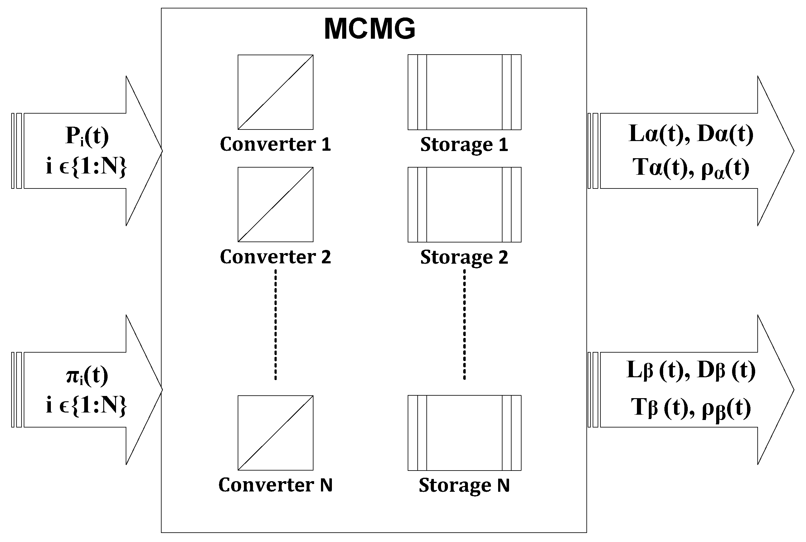
In this paper, the MCE system concept is used to model the proposed MCMG as depicted in Figure 3. The MCE system is, as its name implies, a system that encompasses various energies and energy interactions in addition to the energy-saving conceivable within it [12]. Figure 5 shows a hybrid EH system that can represent the MCMG network as an input and output port of the carriers. The main aim of static planning in this work is to choose the best components while the equality and non-equality constraints are satisfied. The illustrated grid is connected to the electric and natural gas main grid and the purchasing or selling of electricity from/to the main grid is feasible as well. Moreover, the surplus heat can be sold to the district heat network.
The amount of non-responsive and responsive loads for the planning horizon is, respectively, defined as below.
where and are the summation of all non-responsive/responsive loads in MCMG for electrical and thermal consumption at each hour, day, month and year, respectively. To prevent the confusion in case the symbols in parentheses are not described, they are described as , , , and years, month, day, and hour.
3.1. Energy Hub Modeling
In this paper, the proposed MCMG inspires the energy-hub system model. The matrix’s model of energy balancing in the input and the output hub ports is based on the mounted components at given intervals, which are described as:
In this paper, , , , , and describe transferred energy, converter coupling matrix, renewable generation, storage coupling factor and the differential of state of charge in storages, respectively. describes the amount of standby energy losses in energy storages. Owing to the chosen and the installed components for the proposed MCMG, the controllable/non-controllable forecasted loads need to be satisfied over the planning horizon. Electricity and heat balance in the proposed MCMG are, respectively, modeled as follows:
, , , and are the electrical transferred energy, generated energy by CHP, transformer, photovoltaic panel, and equivalent storage electrical flows in electrical energy storage. The footnotes and denote the electrical and thermal type of energies, so that the variables in Equation (6) are the same as the difference of thermal energy types. is the amount of heat generated by selected boiler at each hour, day, month, and year. Energy injection or export to/from the storages are formulated in the Equations (7)–(12), in which Equations (7) and (8) describe equivalent storage flows that are directly related to the storage energy derivatives as modeled in Equations (9)–(12).
where and are binary variable for energy charging or discharging mode in electrical and thermal energy storages, respectively. , , and are the parameters of charge or discharge efficiency in electrical and thermal storage system, respectively.
3.2. Demand Side Management (DSM) Model
Responsive loads are enabled users that are encouraged or rarely forced by the DSM policy to curtail or shift their demands, often optionally, to other hours [49]. The DSM program is classified into two policies based on price or encouragement and penalty. In the first case, the demand is changed based on energy prices in each interval; this policy is used in this paper. Since the energy prices in the input port of the MCMG are specified while the load is supplied by different equipment, it is required to model the final energy price (FEP) of different carriers in the output port of the system. In this case, the final energy prices of electric and heat carriers in the system output are determined based on input energy, equipment efficiency, and operation. The final energy prices of electrical and thermal responsive loads are, respectively, modeled in Equations (13) and (14), based on Figure 5.
and are the final energy price of electrical and thermal responsive loads, respectively. and describe the amount of purchased or received energy (: energy material) at hour and energy purchase price at hour . , , , and are non-responsive and responsive loads for carrier and at hour , respectively. , , , and are the transferred energy and equivalent storage power flows for carrier and at hour , respectively. The electrical (assumed carrier ) and thermal (assumed carrier ) efficiency of CHP are symbolized as and .
Considering the final energy price for the responsive loads, the elasticity matrix that indicates the load-change percentage in proportion to the price-change percentage, is shown in Equations (15) and (16). The diagonal elements of the mentioned matrix are positive and the other elements are negative, i.e., with the price increase in an hour, the responsive load would decrease at the moment and it would shift a share of its demand to the other hours.
where is the elasticity matrix of responsive loads for carrier . With regard to the elasticity matrix definition, the responsive load is modeled as shown below:
In Equation (17), is the initial consumption of carrier , which is changing in proportion to the primary price of carrier at an interval of . is the base energy price of responsive load at hour . The design and structure of the MCMG are modeled according to the load growth over the planning horizon and the selection of the proper components for the proposed system. Owing to energy changes in the output port of the MCMG, the new modified consumption of these responsive customers and the inconstant final energy prices are modeled and obtained as follows:
, , , and denote the received and energy purchased price for electrical and natural gas energies at each hour, day, month and year, respectively. and are binary variables which stands for the selected transformer and CHP in MCMG. is dispatch factor which defines the percentage of natural gas consumption by CHP.
3.3. Net Zero Emission Balance Constraint
The NZE of the PV modules () are modeled over the whole lifetime of modules as shown below.
where and denote the embodied and avoided NZE of PV modules. Since the PV modules affect the emission balance of the MG, therefore, the NZE balance in a network is modeled over the whole lifetime of microgrid (MG) in Equation (24), where the total embodied emissions of the network () and the operational emissions () are taken into account. The NZE balance is acquired if it is zero or lower. The describes how the PV modules effect the emission balance of the network.
where is avoided NZE of the network.
3.4. Objective Function (OF) and Constraints
According to the planning of the MCMG that has been mentioned in the previous parts, all the equations related to the MCMG are provided as EH system concepts. The objective function is modeled in Equation (25) in order to minimize the investment, operation, and maintenance costs. The operation and the maintenance costs are calculated on the basis of NPV. The investment and the operation (fuel and maintenance) costs are given in Equations (26)–(28), respectively. Owing to the mounted energy storage elements and its significant role in the proposed MCMG, the chronological load curves are utilized.
, , and are the investment, operational and maintenance costs, respectively.
The OF equation details are precisely provided as follows:
where , , , and describe the investment cost of CHP, transformer, boiler, and PV module for each candidate (). On the other hand, , , , and are binary variables for each candidate of elements to be chosen or not. Parameter describes the annual interest rate. , , , and are the maintenance coefficient for CHP, boiler, transformer, and PV module, respectively. Generation of each selected component is modelled as follows:
The amount of NZE in the proposed MCMG is determined using the emission conversion factors in Equations (34) and (35), respectively, which are considered as constrains in this paper.
, , and are emission conversion factors for received electricity, natural gas, and PV generation. Owing to the capacity of each component, the energy flows through each of the converters needs to be limited within allowable ranges. The equality and non-equality constraints, such as the allowable range and initial values of variables, are subjected as follows:
4. Solution Method
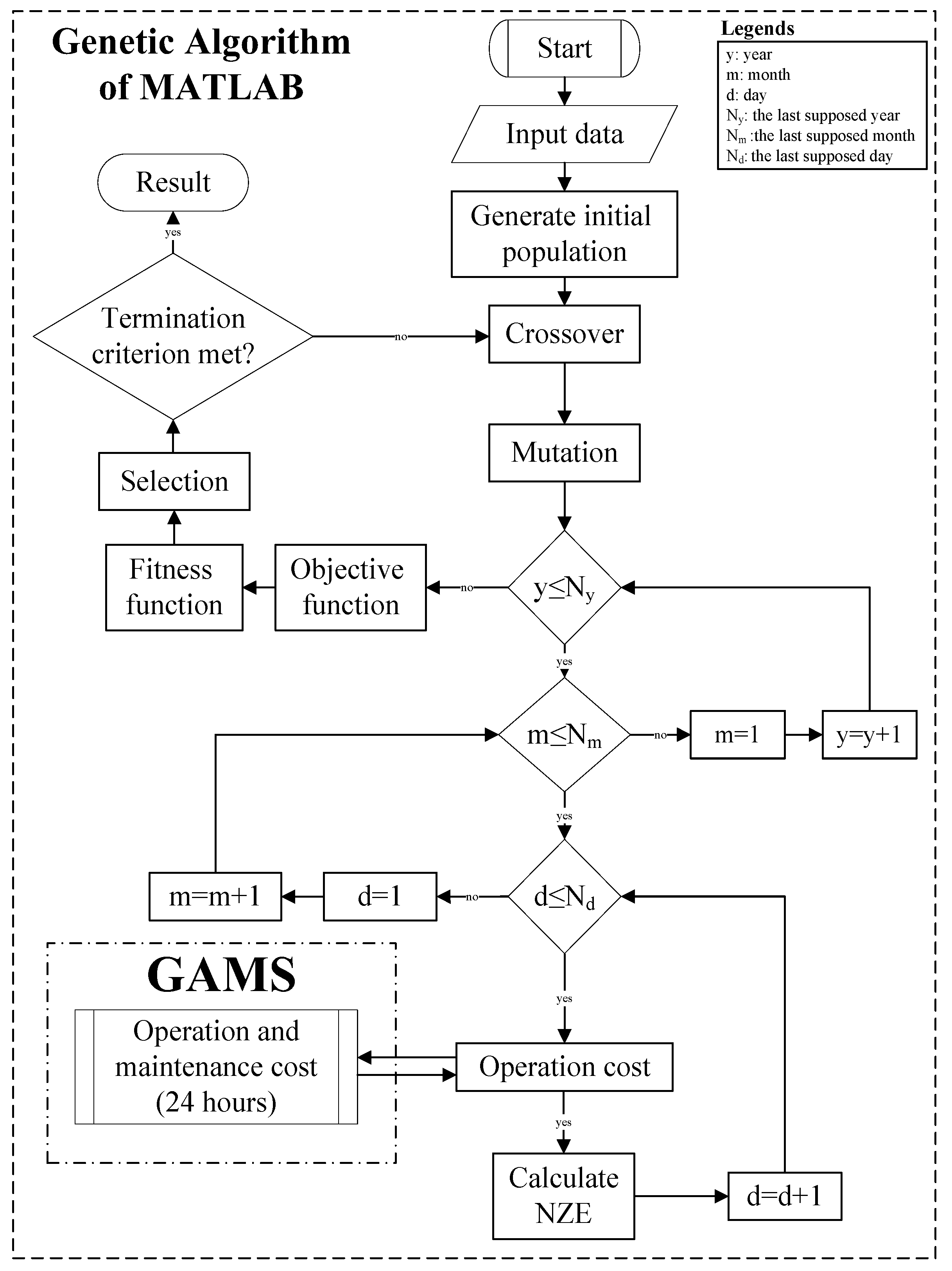
The main goal of the proposed modeling is to determine the appropriate type and size of element while the NZE constraint is met. The flowchart of the optimization method for the MCMG (based on the genetic algorithm of MATLAB and MINLP model of GAMS) is shown in Figure 6; the detailed procedures are described as follows:
- System initialization: The parameters of the genetic algorithm and elements’ characteristics are read as the first step. Generate initial population: A random set of numbers for each chromosome, which each gene fills randomly (between zero and the population of the element’s candidate), acts as the initial population.
- Crossover and mutation application: The crossover and mutation operates to initialize and add a new chromosome to the initial population.
- GAMS optimization software runs to calculate operation, maintenance costs, and NZE: The operation and maintenance cost in addition to the NZE is calculated in a loop until the maximum number of years, months, and days by the user is reached.
- Fitness function evaluation: After the objective function is obtained, the fitness value of each chromosome is evaluated.
- Sorting out the initial population: The initial and best population from the lowest to the highest are sequentially sorted. The first one is the most appropriate in the population.
- Stopping criterion: If the maximum number of iterations is reached, the execution stops. Otherwise, the execution needs to restart from Step 3.
5. Simulation Results and Discussion
The model presented in this paper has been applied to a farm as an MCMG to illustrate the performance of the proposed method. The proposed MCMG design in the electricity, gas, and district heat grid-connected mode are depicted in Figure 3. The proposed method determines the best operational point of the MCMG and the optimal type and size of its elements with the minimum net present cost when NZE constraint is reached during its life circle. A set of four elements comprising the transformer, the CHP, the boiler, and the PV are considered while the energy storage elements with their predetermined sizes are mounted in the network. Each element has five different candidates, which are classified according to different capacities, efficiencies, investments, installation costs, and the maintenance cost coefficient (see Table 1). The properties of the energy storage elements are stated in Table 2.
It is important to mention that the model structure can contain either one candidate of each set or none. Furthermore, there are no restrictions to the annual investment. The planning problem is performed for a five-year planning horizon, and the investment and operation costs are analyzed on the basis of the net present value so that all the costs are transferred to the first year using the interest rate (IR) value. The investment and the installation costs are assumed to be incurred during the first year of the planning horizon. In addition, it is assumed that the load and the energy prices will be increased every year; therefore, the annual load growth rate and the energy price growth rate are provided for an operational period of five years as shown in Table 3.
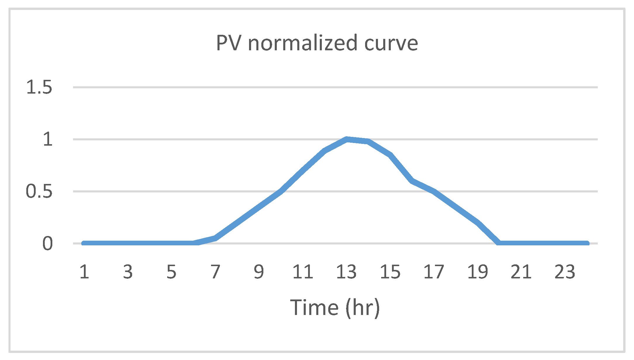
The conversion factors of electricity, natural gas from the grid, and the PV generation for NZE calculation are equal to 0.40957, 0.20444, and 0.46, respectively. These factors are reported in [50]. The purchase and the sale prices of carriers are assumed in Figure 7, which are considered similar for each season, but they are increasing year by year due to energy price growth rates. The normalized PV generation curve on a summer day is provided in Figure 8. In order to simplify and lower the computational burden of PV generation, its generation is assumed to be similar for all the days in the planning horizon.
In this paper, two typical daily-energy curves—one for the working-day and one for the off-day (controllable/non-controllable electricity and heat demands)—in a 24 h interval are considered differently for each season due to the similar behavior of each daily energy consumption in each season. Summer and winter are considered as two typical seasons for 12-month periods. In order to give a hint to the readers and avoid excess figures of energy consumptions, the average amount of electrical and thermal consumption in a farm is given which are almost equal to 400 KWh in the first year. Table 4 demonstrates the optimized elements and characteristics of the MCMG; the display of the MCMG structure is schematically depicted in Figure 9.
The confusing query here is whether or not the components are chosen optimally for efficient long-term planning. This issue can be simply conveyed and answered by looking back more intently at Table 1 and Table 4. The result shows that the transformer type 1 has been selected because of its lower investment cost and its higher efficiency in comparison to the other units. Owing to higher electrical rather than thermal demand, the CHP type 3 is selected due to its high power-to-heat ratio, whereas the boiler type 1 is chosen because of its low investment cost and high efficiency to fulfill a small share of demands. The PV type 4 is chosen due to the zero-energy generation cost of this unit and the adequate capacity in proportion to its appropriate and rational efficiency, and its investment cost. It needs to be mentioned that these elements are chosen in case the NZE constraint (“NZE must be less or equal zero”) over the planning horizon is met.
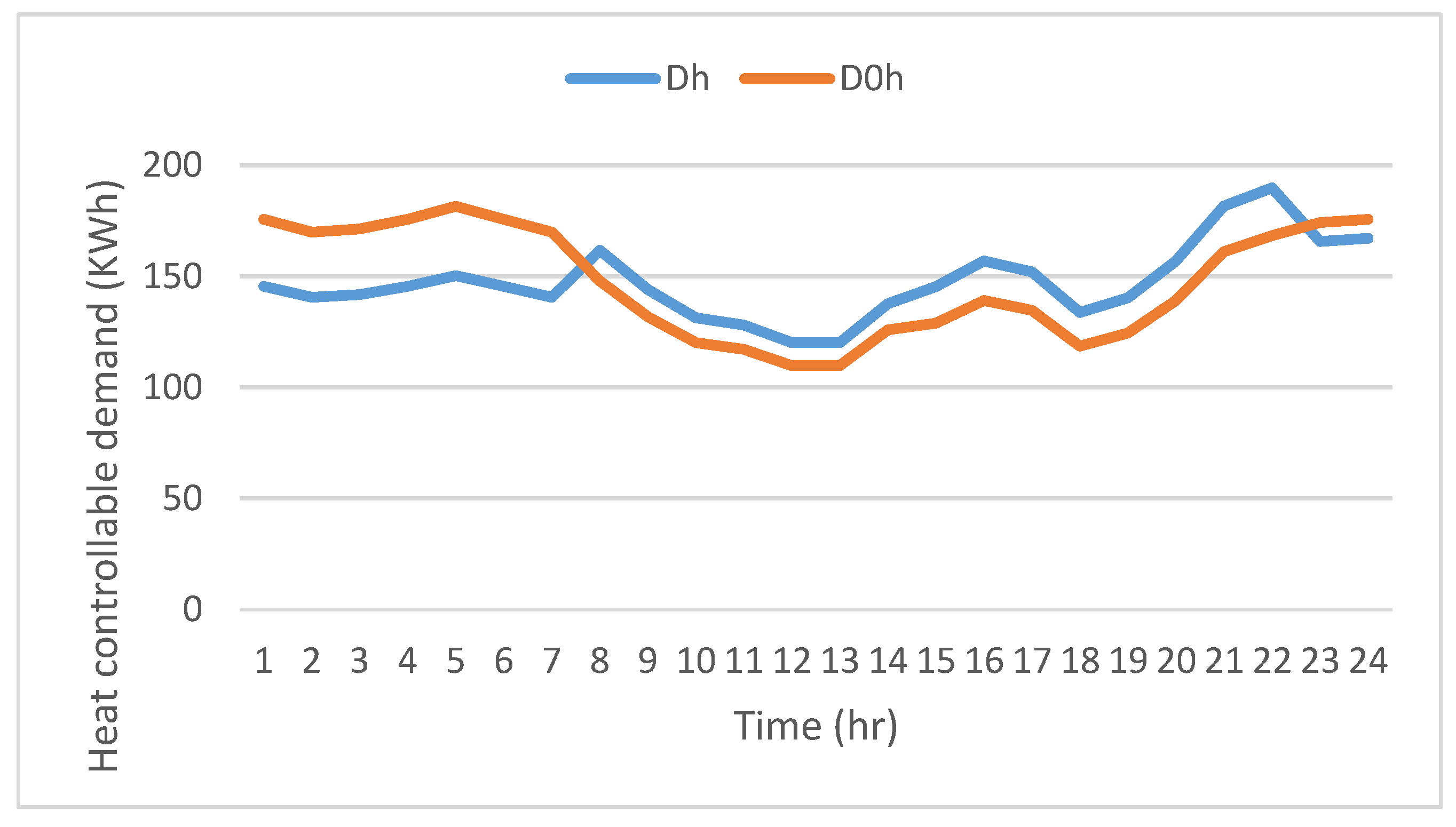
The operational optimization results are shown in Figure 10, Figure 11, Figure 12, Figure 13, Figure 14, Figure 15 and Figure 16. The electrical and thermal controllable loads form a small part of the total load as is observable in Figure 10 and Figure 11, respectively. These responsive loads are encouraged or forced to shift their demand in the peak intervals to off-peak intervals. The peak period for the electrical load is considered between the Intervals 15–22, whereas the thermal load is in the intervals 1–7 and 23–24.
The base and final energy prices of electricity and the heat for responsive loads are obtained and illustrated in Figure 12. It can be observed that the final energy price of electrical responsive load are lower than its base price at some intervals because of RERs generation, which has led to less power purchasing from the upstream grid. This circumstance results in the electricity purchase price increasing at these intervals, despite the fact that the DR program would have decreased consumption. On the other hand, the final energy price of heat for responsive loads is higher than its base prices in all the intervals as a result of not receiving low-price heat.
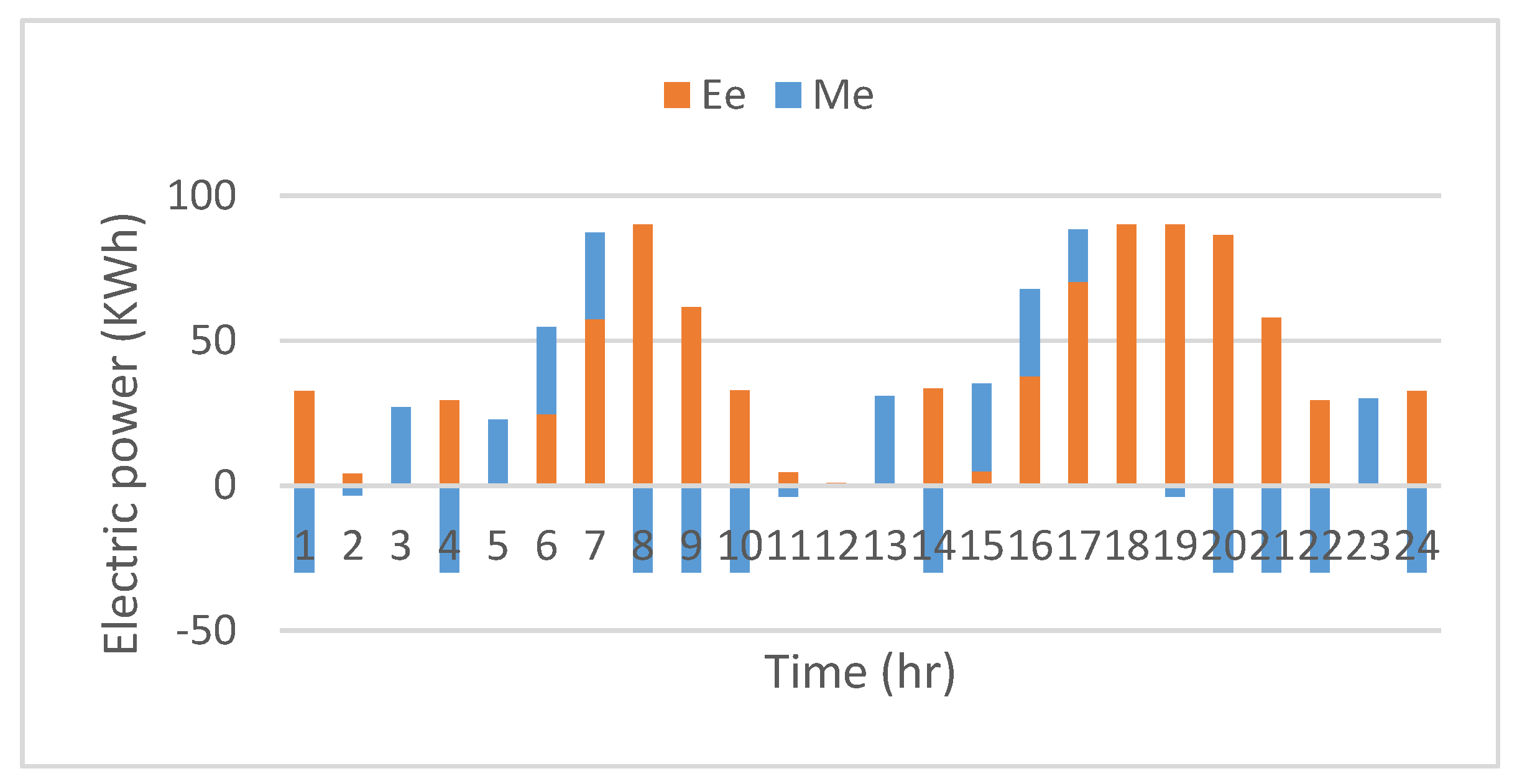
The energy storage element provides economic benefits, an improvement in reliability indices, and also handles the intermittency of the RERs [46]. The equivalent storage power flows and the state of charge (SOC) of the electric and the heat storages are illustrated in Figure 13 and Figure 14, respectively.
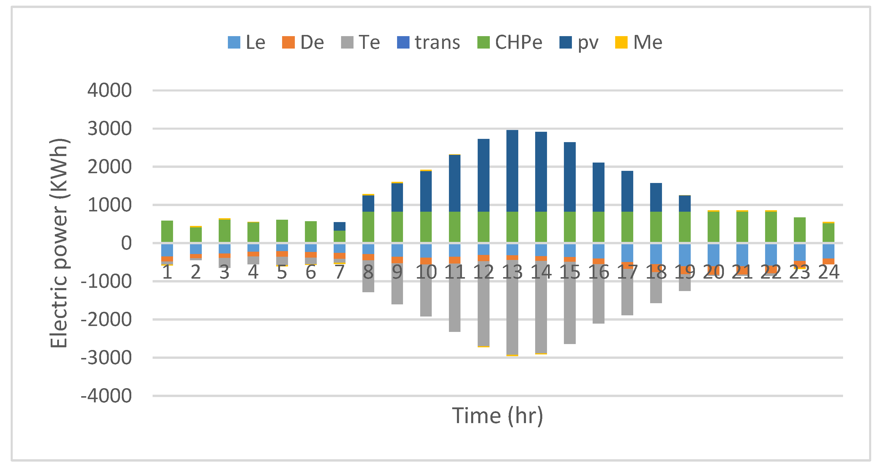
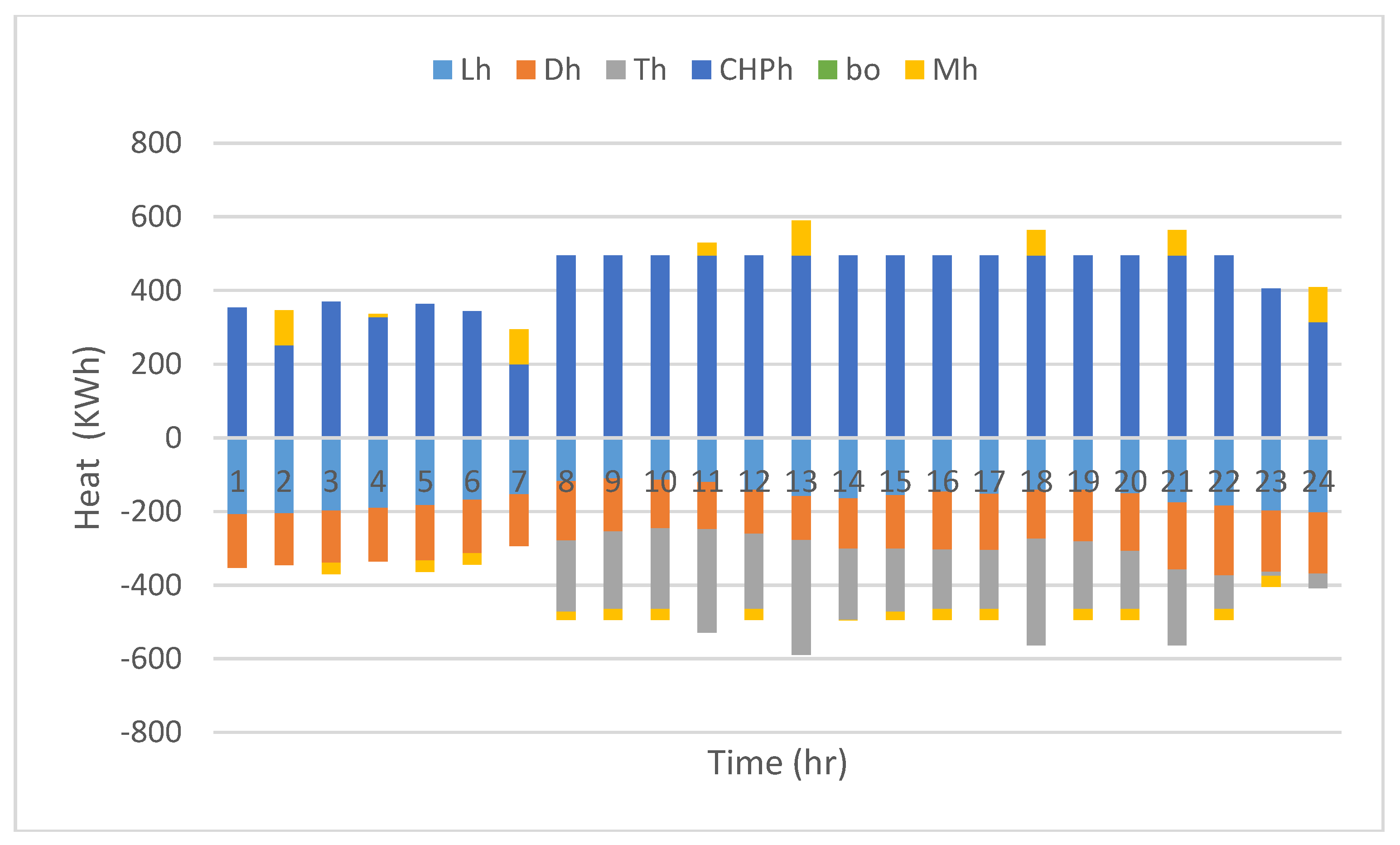
The electrical and the heat load balancing in a structured MCMG are shown in Figure 15 and Figure 16, respectively. In the winter working-day of the 5th year, the electricity purchase from the grid and the boiler generation are equal to zero for all the intervals, while the CHP fulfills most of the electrical and heat demands, and allows the sale of surplus energy to the main grid because of profitable-energy trading. More importantly, a big share of electrical demand is fulfilled by the RERs and the rest of it are stored or sold to the main grid. A detailed explanation of the results is, however, difficult to achieve due to the complexity of the problem.
Finally, the total NPV cost of the MCMG’s operation for all the planned years and the investment cost of the chosen elements that are installed in the first year are listed in Table 5. Moreover, the amount of NZE for each year is calculated in Table 6, which is increasing year by year due to load growth. Furthermore, three scenarios for investigating the impact of the electrical storage element on the total NPV cost and the NZE amounts are carried out, whose result are listed in Table 7. It can be inferred from Table 7 that increasing the capacity of electrical storages and the inverters lead to less total cost, and affect the NZE amount.
6. Conclusions
This paper proposed a long-term multi-carrier microgrid expansion planning model in the electricity, natural gas, and district heat grid-connected mode by considering the net zero emission constraints over the planning horizon. The appropriate type and size of elements that are to be installed in the 1st year of the planning horizon are planned and designed, whereas the optimal dispatching of the chosen elements includes the transformer, CHP, boiler, and PV with the existence of energy storage systems and responsive loads that are operated. The objective is to evaluate and minimize the total NPV cost, including investment, operation, and maintenance while the NZE constraint is satisfied. To solve the problem, a compound solution method using the genetic algorithm of MATLAB and the MINLP of the GAMS software are employed. The proposed model is tested on a single-bus MCMG and the numerical results demonstrate the use and the potential application of the model.
Current and future work is dedicated to model the proposed system with regard to the uncertainties of renewable energy resources, loads, and energy tariffs to gain more accurate optimal results. Adding a wind turbine to the system can help in attaining better economic and environmental performance (i.e., lower pollution). Meanwhile, the reliability of MCMG can also be the subject of important research.
Acknowledgments
The authors received no specific funding for this work.
Author Contributions
The main part of the paper is written, designated and analyzed by Vahid Amir while Shahram Jadid and Mehdi Ehsan took on the roles of consultants and corrected the paper in order that it should be written and submitted properly for publications. Moreover, the proper modeling of the problem and the results have been checked by Shahram Jadid and Mehdi Ehsan.
Conflicts of Interest
The authors declare no conflict of interest.
References
- Shahmohammadi, A.; Dalvand, M.M.; Ghazizadeh, M.S.; Salemnia, A. Energy hubs’ structural and operational linear optimization with energy storage elements. In Proceedings of the 2nd International Conference on Electric Power and Energy Conversion Systems, Sharjah, UAE, 15–17 November 2011. [Google Scholar]
- An, S.A.S.; Li, Q.L.Q.; Gedra, T.W. Natural gas and electricity optimal power flow. In Proceedings of the 2003 IEEE PES Transmission and Distribution Conference and Exposition, Dallas, TX, USA, 7–12 September 2003; Volume 1, pp. 138–143. [Google Scholar] [CrossRef]
- Gil, E.M.; Quelhas, A.; McCalley, J.; Voorhis, T.V. Modeling integrated energy transportation networks for analysis of economic efficiency and network interdependencies. In Proceedings of the 35th North American Power Symposium, Manhatan, KS, USA, 22–24 September 2003. [Google Scholar]
- Bakken, B.H.; Holen, A.T. Energy service systems: Integrated planning case studies. In Proceedings of the IEEE Power Engineering Society General Meeting, Denver, CO, USA, 6–10 June 2004. [Google Scholar]
- De Melllo, O.D.; Ohishi, T. An Integrated Dispatch Model of Gas Supply and Thermoelectric Systems. In Proceedings of the 15th Power Systems Computation Conference, Liège, Belgium, 22–26 August 2005; pp. 1–7. [Google Scholar]
- Shahidehpour, M.; Fu, Y.; Wiedman, T. Impact of Natural Gas Infrastructure on Electric Power Systems. Proc. IEEE 2005, 93, 1042–1056. [Google Scholar] [CrossRef]
- Geidl, M.; Andersson, G.G. Optimal power flow of multiple energy carriers. IEEE Trans. Power Syst. 2007, 22, 145–155. [Google Scholar] [CrossRef]
- Geidl, M.; Andersson, G. Operational and structural optimization of multi-carrier energy systems. Eur. Trans. Electr. Power 2006, 16, 463–477. [Google Scholar] [CrossRef]
- Krause, T.; Andersson, G.; Fröhlich, K.; Vaccaro, A. Multiple-energy carriers: Modeling of production, delivery, and consumption. Proc. IEEE 2011, 99, 15–27. [Google Scholar] [CrossRef]
- Geidl, M.; Koeppel, G.; Favre-Perrod, P.; Klöckl, B.; Andersson, G.; Fröhlich, K. Energy hubs for the future. IEEE Power Energy Mag. 2007, 5, 24–30. [Google Scholar] [CrossRef]
- Liu, C.; Shahidehpour, M.; Wang, J. Coordinated scheduling of electricity and natural gas infrastructures with a transient model for natural gas flow. Chaos 2011, 21, 25102. [Google Scholar] [CrossRef] [PubMed]
- Sheikhi, A.; Ranjbar, A.M.; Oraee, H. Financial analysis and optimal size and operation for a multicarrier energy system. Energy Build. 2012, 48, 71–78. [Google Scholar] [CrossRef]
- Moeini-Aghtaie, M.; Abbaspour, A.; Fotuhi-Firuzabad, M.; Hajipour, E. A decomposed solution to multiple-energy carriers optimal power flow. IEEE Trans. Power Syst. 2014, 29, 707–716. [Google Scholar] [CrossRef]
- Geidl, M. Integrated Modeling and Optimization of Multi-Carrier Energy Systems; ETH: Zürich, Switzerland, 2007. [Google Scholar]
- Geidl, M.; Andersson, G. Optimal coupling of energy infrastructures. In Proceedings of the 2007 IEEE Lausanne Power Tech, Lausanne, Switzerland, 1–5 July 2007; pp. 1398–1403. [Google Scholar]
- Shahmohammadi, A.; Moradi-Dalvand, M.; Ghasemi, H.; Ghazizadeh, M.S. Optimal Design of Multicarrier Energy Systems Considering Reliability Constraints. IEEE Trans. Power Deliv. 2015, 30, 878–886. [Google Scholar] [CrossRef]
- Mohsenzadeh, A.; Ardalan, S.; Haghifam, M.-R.; Pazouki, S. Optimal place, size, and operation of combined heat and power in multi carrier energy networks considering network reliability, power loss, and voltage profile. IET Gener. Transm. Distrib. 2016, 10, 1615–1621. [Google Scholar] [CrossRef]
- Moradi, H.; Abtahi, A.; Esfahanian, M. Optimal energy management of a smart residential combined heat, cooling and power. Int. J. Tech. Phys. Probl. Eng. 2016, 8, 9–16. [Google Scholar]
- Zhang, X.; Shahidehpour, M.; Alabdulwahab, A.; Abusorrah, A. Optimal Expansion Planning of Energy Hub with Multiple Energy Infrastructures. IEEE Trans. Smart Grid 2015, 6, 2302–2311. [Google Scholar] [CrossRef]
- Bahramirad, S.; Reder, W.; Khodaei, A. Reliability-Constrained Optimal Sizing of Energy Storage System in a Microgrid. IEEE Trans. Smart Grid 2012, 3, 2056–2062. [Google Scholar] [CrossRef]
- Seifi, H.; Sepasian, M.S. Electric Power System Planning: Issues, Algorithms and Solutions. Power Syst. 2011, 49. [Google Scholar] [CrossRef]
- Hemmes, K.; Zachariah-Wolf, J.L.; Geidl, M.; Andersson, G. Towards multi-source multi-product energy systems. Int. J. Hydrog. Energy 2007, 32, 1332–1338. [Google Scholar] [CrossRef]
- Geidl, M.; Andersson, G. Operational and topological optimization of multi-carrier energy systems. In Proceedings of the 2005 International Conference on Future Power Systems, Amsterdam, The Netherlands, 18 November 2005. [Google Scholar]
- Moeini-Aghtaie, M.; Dehghanian, P.; Fotuhi-Firuzabad, M.; Abbaspour, A. Multiagent Genetic Algorithm: An Online Probabilistic View on Economic Dispatch of Energy Hubs Constrained by Wind Availability. IEEE Trans. Sustain. Energy 2014, 5, 699–708. [Google Scholar] [CrossRef]
- Hajimiragha, A.; Canizares, C.; Fowler, M.; Geidl, M.; Andersson, G. Optimal Energy Flow of integrated energy systems with hydrogen economy considerations. In Proceedings of the 2007 iREP Symposium—Bulk Power System Dynamics and Control—VII. Revitalizing Operational Reliability, Charleston, SC, USA, 19–24 August 2007; pp. 1–11. [Google Scholar]
- Ramirez-Elizondo, L.M.; Paap, G.C. Unit commitment in multiple energy carrier systems. In Proceedings of the 41st North American Power Symposium, Starkville, MS, USA, 4–6 October 2009; pp. 1–6. [Google Scholar]
- Ramirez-Elizondo, L.; Velez, V.; Paap, G.C. A technique for unit commitment in multiple energy carrier systems with storage. In Proceedings of the 2010 9th Conference on Environment and Electrical Engineering, Prague, Czech Republic, 16–19 May 2010; pp. 106–109. [Google Scholar]
- Geidl, M.; Andersson, G. Optimal power dispatch and conversion in systems with multiple energy carriers. In Proceedings of the Power Systems Computation Conference, Liege, Belgium, 22–26 August 2005; pp. 22–26. [Google Scholar]
- Ganesan, S.; Padmanaban, S.; Varadarajan, R.; Subramaniam, U.; Mihet-Popa, L. Study and Analysis of an Intelligent Microgrid Energy Management Solution with Distributed Energy Sources. Energies 2017, 10, 1419. [Google Scholar] [CrossRef]
- Moradi, H.; Esfahanian, M.; Abtahi, A.; Zilouchian, A. Modeling a Hybrid Microgrid Using Probabilistic Reconfiguration under System Uncertainties. Energies 2017, 10, 1430. [Google Scholar] [CrossRef]
- Roh, J.H.; Shahidehpour, M.; Wu, L. Market-based generation and transmission planning with uncertainties. IEEE Trans. Power Syst. 2009, 24, 1587–1598. [Google Scholar] [CrossRef]
- Sheikhi, A.; Ranjbar, A.M.; Safe, F.; Mahmoodi, M. CHP optimized selection methodology for an energy hub system. In Proceedings of the 2011 10th International Conference on Environment and Electrical Engineering, Rome, Italy, 8–11 May 2011; pp. 1–5. [Google Scholar]
- Sheikhi, A.; Ranjbar, A.M.; Oraee, H.; Moshari, A. Optimal Operation and Size for an Energy Hub with CCHP. Energy Power Eng. 2011, 3, 641–649. [Google Scholar] [CrossRef]
- Andersson, G. The influence of combined power, gas, and thermal networks on the reliability of supply. In Proceedings of the Sixth World Energy System Conference, Torino, Italy, 10–12 July 2006. [Google Scholar]
- Koeppel, G.; Andersson, G. Reliability modeling of multi-carrier energy systems. Energy 2009, 34, 235–244. [Google Scholar] [CrossRef]
- Ren, H.; Gao, W. A MILP model for integrated plan and evaluation of distributed energy systems. Appl. Energy 2010, 87, 1001–1014. [Google Scholar] [CrossRef]
- Arcuri, P.; Florio, G.; Fragiacomo, P. A mixed integer programming model for optimal design of trigeneration in a hospital complex. Energy 2007, 32, 1430–1447. [Google Scholar] [CrossRef]
- Baghernejad, A.; Yaghoubi, M.; Jafarpur, K. Exergoeconomic optimization and environmental analysis of a novel solar-trigeneration system for heating, cooling and power production purpose. Sol. Energy 2016, 134, 165–179. [Google Scholar] [CrossRef]
- Salimi, M.; Adelpour, M.; Vaez-ZAdeh, S.; Ghasemi, H. Optimal planning of energy hubs in interconnected energy systems: A case study for natural gas and electricity. IET Gener. Transm. Distrib. 2015, 9, 695–707. [Google Scholar] [CrossRef]
- Intergovernmental Panel on Climate Change (IPCC). Climate Change 2014 Synthesis Report Summary Chapter for Policymakers, Intergovernmental Panel on Climate Change; IPCC: Geneva, Switzerland, 2014; Volume 31. [Google Scholar]
- Carbon Tracker Initiative Unburnable Carbon 2013: Wasted Capital and Stranded Assets. 2013. Available online: https://www.carbontracker.org/ (accessed on 13 August 2017).
- Cleveland, S. Carbon asset Risk: From rhetoric to action. In Proceedings of the Smith School Stranded Assets Conference, Oxford, UK, 24 September 2015. [Google Scholar]
- Marszal, A.J.; Heiselberg, P.; Bourrelle, J.S.; Musall, E.; Voss, K.; Sartori, I.; Napolitano, A. Zero Energy Building—A review of definitions and calculation methodologies. Energy Build. 2011, 43, 971–979. [Google Scholar] [CrossRef]
- Fasihi, M.; Bogdanov, D.; Breyer, C. Renewable Energy-based Synthetic Fuels Export Options for Iran in a Net Zero Emissions World. In Proceedings of the 11th International Energy Conference, Belfast, UK, 31 August–2 September 2016. [Google Scholar]
- Breyer, C.; Gulagi, A.; Fell, H.-J. Sustainable and Low-Cost Energy System for India without Nuclear and Coal Base Load. 2016. Available online: https://www.researchgate.net/profile/Christian_Breyer/publication/308647383_Sustainable_and_Low-Cost_Energy_System_for_India_without_Nuclear_and_Coal_Base_Load/links/57ea0eb808aeb34bc08feda5.pdf (accessed on 13 August 2017).
- Good, C.; Kristjansdottír, T.; Houlihan Wiberg, A.; Georges, L.; Hestnes, A.G. Influence of PV technology and system design on the emission balance of a net zero emission building concept. Sol. Energy 2016, 130, 89–100. [Google Scholar] [CrossRef]
- UNFCCC Conference of the Parties (COP). Adoption of the Paris Agreement. Proposal by the President. In Proceedings of the Paris Climate Change Conference, Paris, France, 30 November–11 December 2015. [Google Scholar]
- Sartori, I.; Napolitano, A.; Voss, K. Net zero energy buildings: A consistent definition framework. Energy Build. 2012, 48, 220–232. [Google Scholar] [CrossRef]
- Sheikhi, A.; Rayati, M.; Bahrami, S.; Ranjbar, A.M. Integrated demand side management game in smart energy hubs. IEEE Trans. Smart Grid 2015, 6, 675–683. [Google Scholar] [CrossRef]
- Government Emission Conversion Factors for Greenhouse Gas Company Reporting—GOV.UK. Available online: https://www.gov.uk/government/collections/government-conversion-factors-for-company-reporting (accessed on 7 January 2017).
Figure 1.
Multi-carrier microgrid (MCMG) structure.

Figure 2.
Sampled MCMG structure.
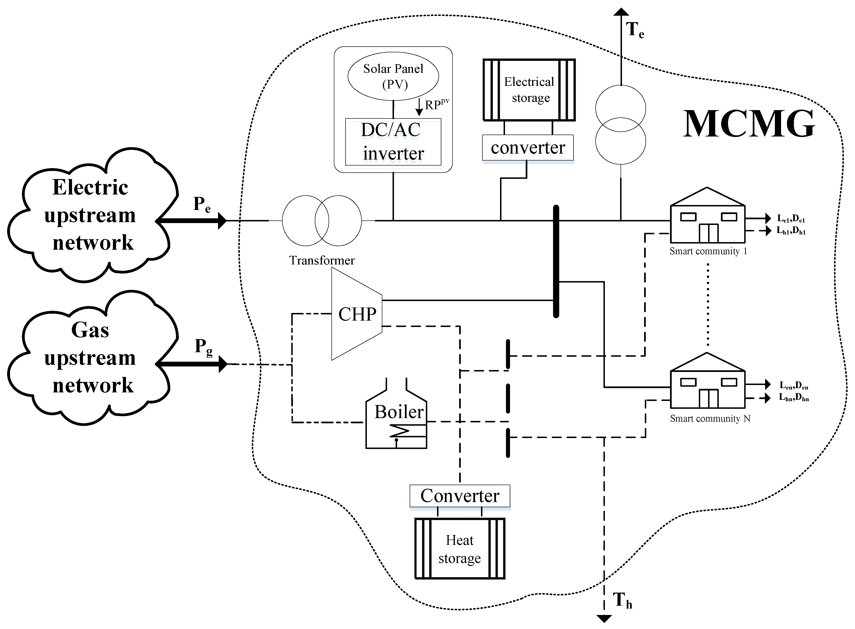
Figure 3.
Desired MCMG for structural and operational optimizations.
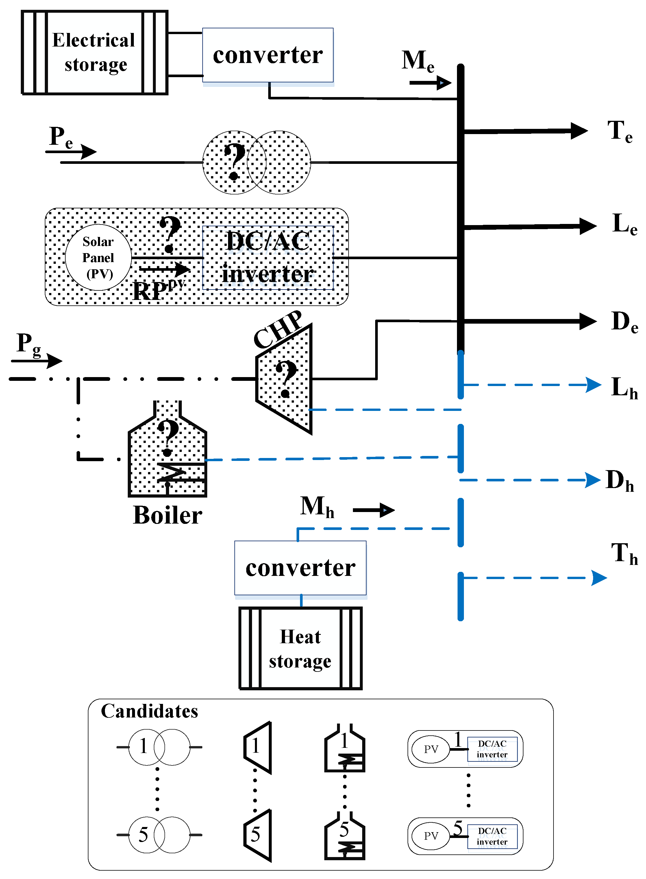
Figure 4.
Schematic drawing of the correlation between MCMG and the energy grids with weighting systems.
Figure 4.
Schematic drawing of the correlation between MCMG and the energy grids with weighting systems.

Figure 5.
Simplified figure of analyzed MCMG (represented as energy hub).

Figure 6.
The flow chart of the optimization algorithm for MCMG.

Figure 7.
Energy prices for the 1st year.
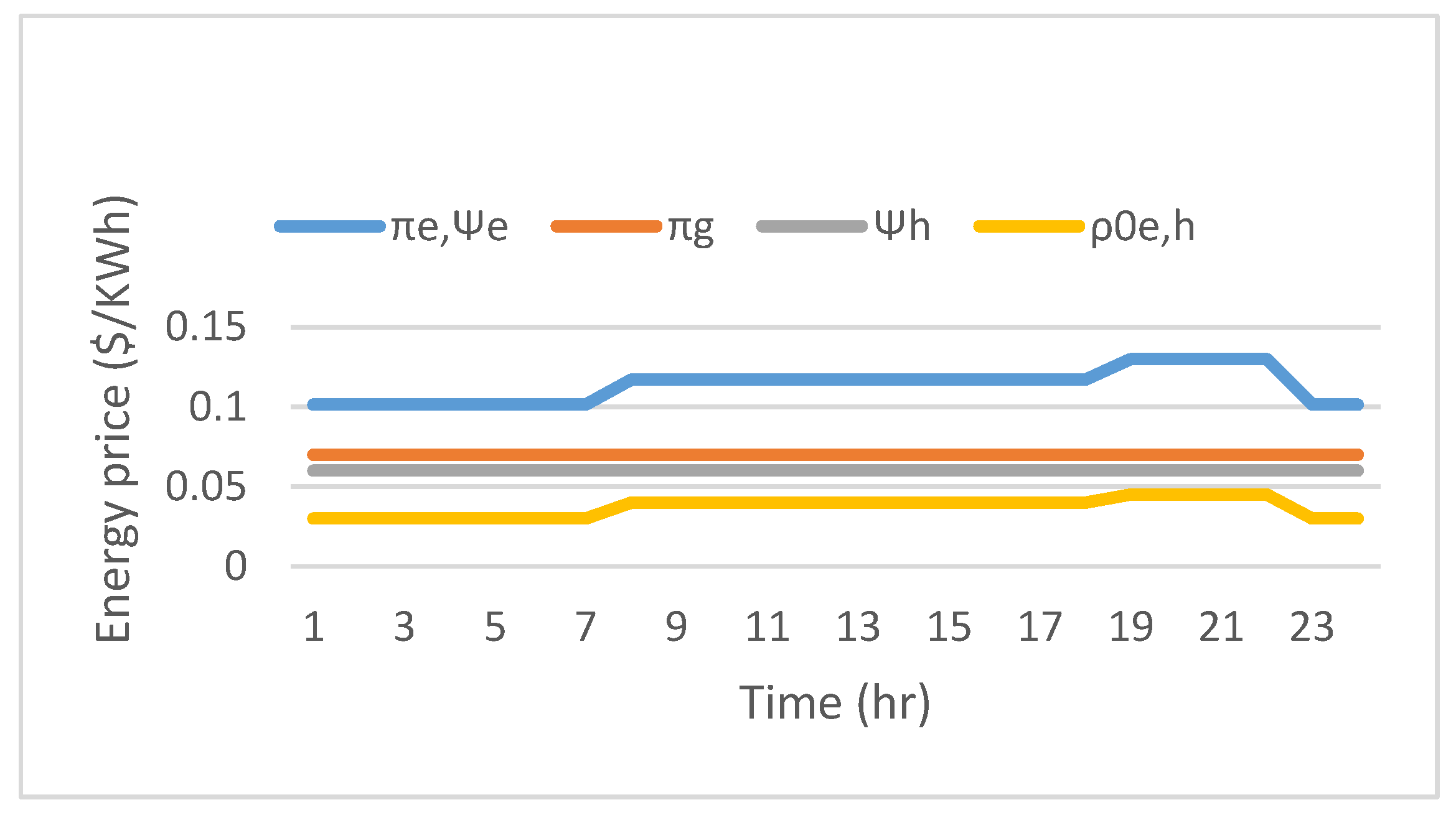
Figure 8.
The normalized PV generation curve on a summer day.

Figure 9.
Design and Structure of proposed MCMG.
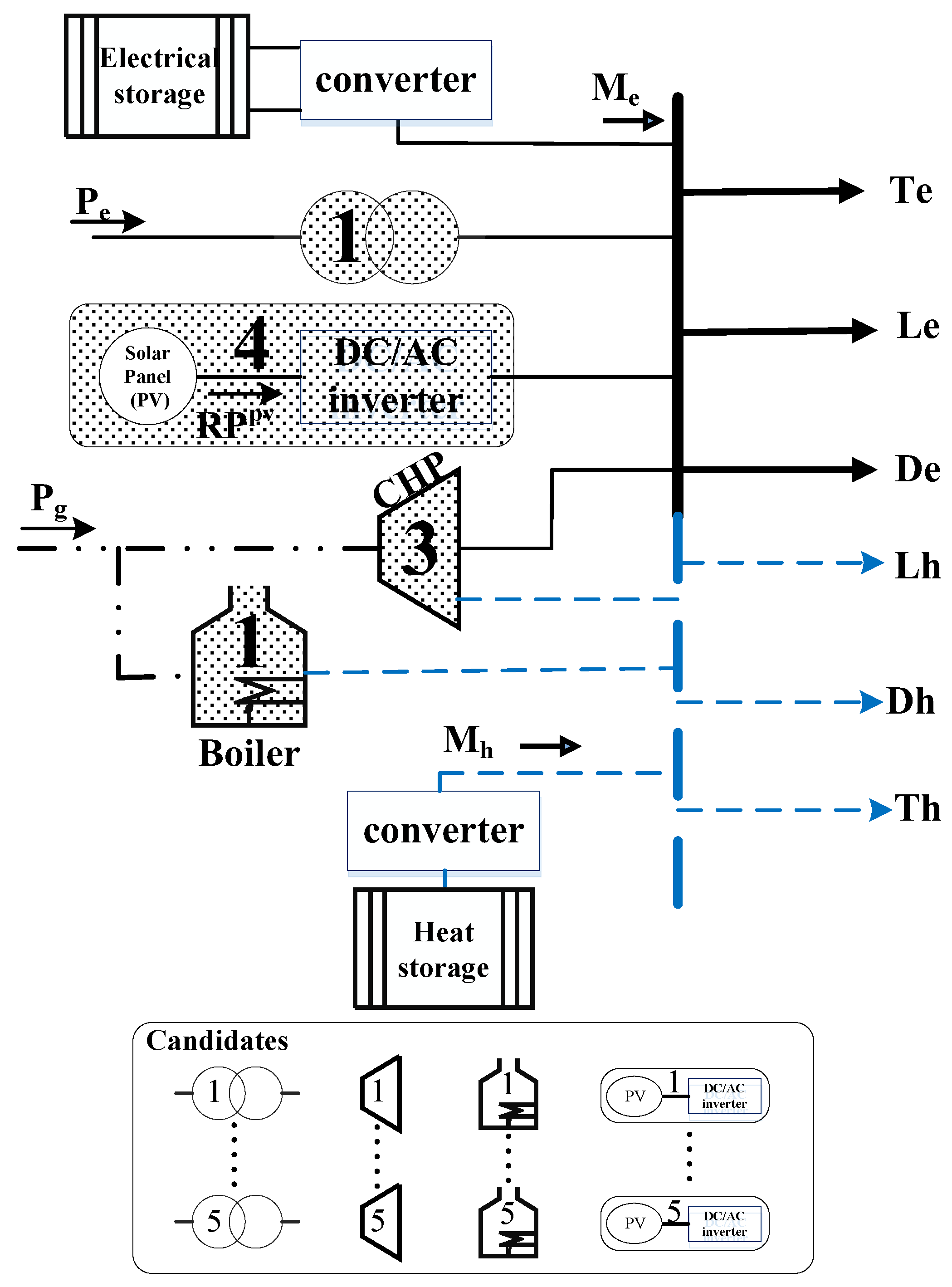
Figure 10.
Electrical responsive load profile under the time of use (TOU) policy in a winter working-day for the last year.
Figure 10.
Electrical responsive load profile under the time of use (TOU) policy in a winter working-day for the last year.

Figure 11.
Thermal responsive load profile under the TOU policy in a winter working-day for the last year.
Figure 11.
Thermal responsive load profile under the TOU policy in a winter working-day for the last year.

Figure 12.
Base and final energy prices of responsive electric and heat loads in a winter off-day for the last year.
Figure 12.
Base and final energy prices of responsive electric and heat loads in a winter off-day for the last year.
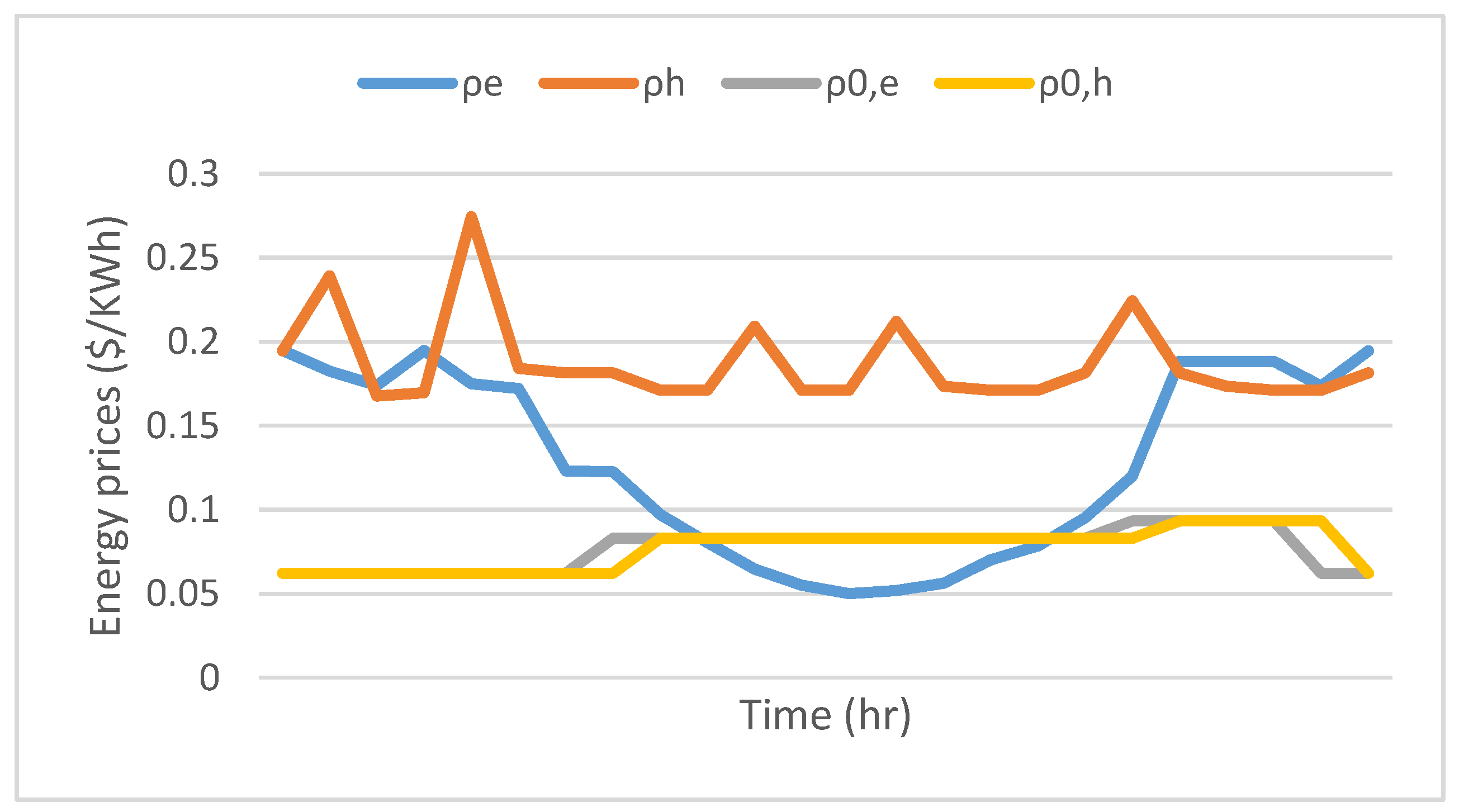
Figure 13.
Equivalent storage electricity flows and the state of charge (SOC) of electrical storage in a winter off-day for the last year.
Figure 13.
Equivalent storage electricity flows and the state of charge (SOC) of electrical storage in a winter off-day for the last year.

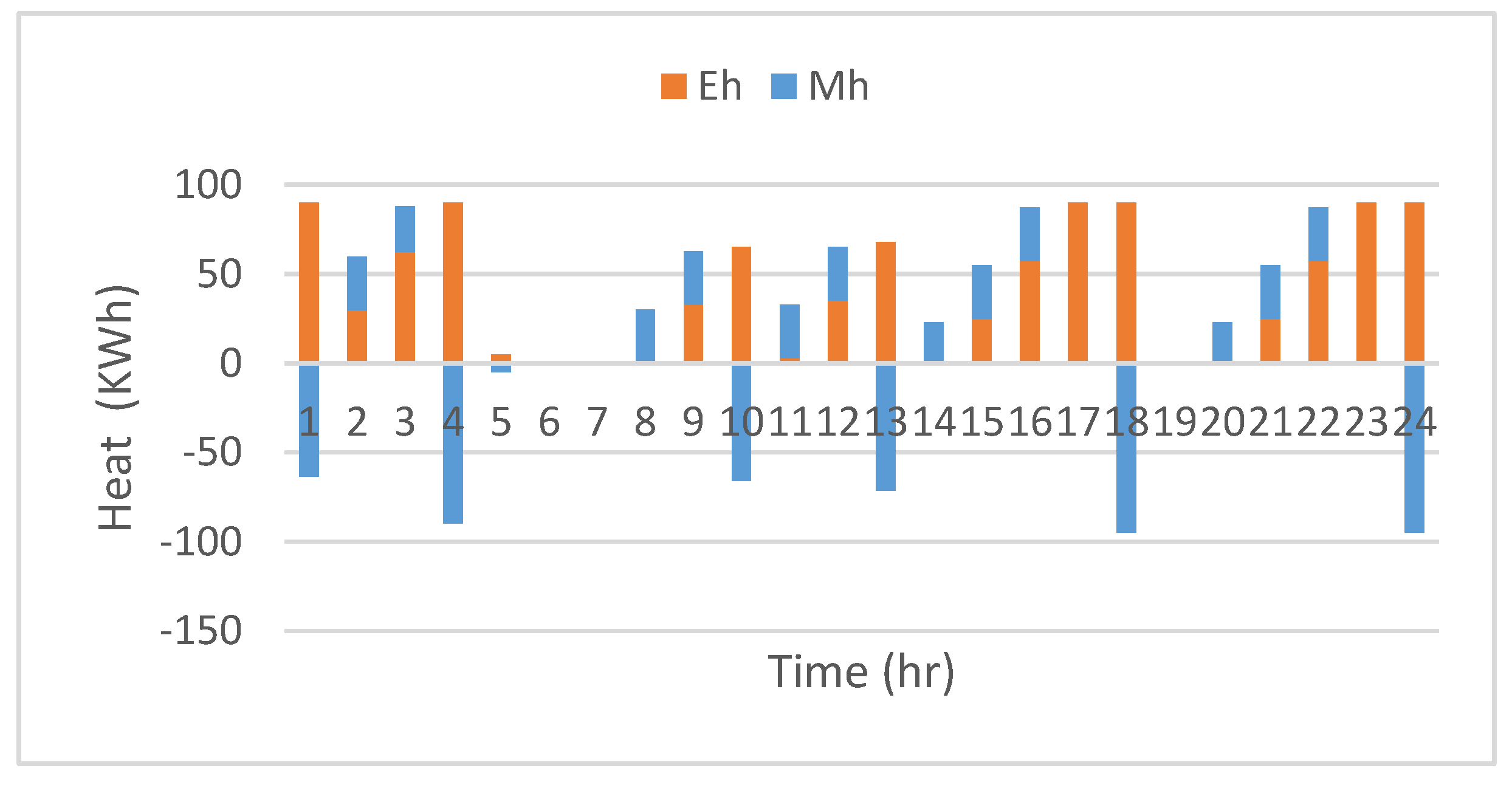
Figure 14.
Equivalent storage heat flows and the SOC of thermal storage in a winter off-day for the last year.
Figure 14.
Equivalent storage heat flows and the SOC of thermal storage in a winter off-day for the last year.

Figure 15.
Electric portion in the MCMG.

Figure 16.
Heat portion in the MCMG.


Table 1.
Technical specification of the candidates.
| Element | Type | Maximum Capacity, KW | Efficiencies in % | Investment & Installation Cost in Million $ | Maintenance Coefficient, $/KWh | ||
|---|---|---|---|---|---|---|---|
| el. | th. | ∑ | |||||
| Transformer | 1 | 800 | 92 | - | 92 | 0.825 | 0.003 |
| 2 | 900 | 90 | - | 90 | 1.328 | 0.0027 | |
| 3 | 1000 | 89 | - | 89 | 1.660 | 0.0024 | |
| 4 | 1500 | 87 | - | 87 | 2.490 | 0.0022 | |
| 5 | 1800 | 85 | - | 85 | 2.988 | 0.002 | |
| CHP | 1 | 500 | 40 | 35 | 75 | 0.221 | 0.015 |
| 2 | 600 | 40 | 44 | 84 | 0.272 | 0.0135 | |
| 3 | 825 | 50 | 30 | 80 | 0.375 | 0.0125 | |
| 4 | 1125 | 40 | 40 | 80 | 0.487 | 0.0115 | |
| 5 | 1350 | 35 | 40 | 75 | 0.600 | 0.01 | |
| Boiler | 1 | 300 | - | 90 | 90 | 0.075 | 0.009 |
| 2 | 450 | - | 87 | 87 | 0.1 | 0.008 | |
| 3 | 600 | - | 85 | 85 | 0.125 | 0.005 | |
| 4 | 750 | - | 83 | 83 | 0.15 | 0.003 | |
| 5 | 900 | - | 80 | 80 | 0.175 | 0.002 | |
| PV | 1 | 2000 | 85 | - | 85 | 2.48 | 0.0014 |
| 2 | 2300 | 82 | - | 82 | 4.852 | 0.0012 | |
| 3 | 2500 | 80 | - | 80 | 3.1 | 0.001 | |
| 4 | 2700 | 79 | - | 79 | 3.348 | 0.001 | |
| 5 | 3000 | 78 | - | 78 | 3.72 | 0.001 | |
CHP: combined heat and power; PV: photovoltaic.
Table 2.
Properties of the energy storage elements.
| Storage Elements | Charge & Discharge Efficiency Rate (%) | Capacity (KW) | Converter Rate Capacity (KWh) | ||
|---|---|---|---|---|---|
| Discharging | Charging | ||||
| Electrical storage | 95 | 92 | 90 | −30 | +30 |
| Thermal storage | 95 | 92 | 90 | −30 | +30 |
Table 3.
Economic parameters.
| Annual Interest Rate (%) | Annual Load Growth Rate (%) | Annual Energy Purchasing Price Growth Rate (%) |
|---|---|---|
| 15 | 10 | 20 |
Table 4.
Characteristic of the chosen elements.
| Element | Maximum Capacity (KW) | Efficiencies (%) | Investment & Installation Cost (Million $) | Maintenance Coefficient ($/KWh) | ||
|---|---|---|---|---|---|---|
| el. | th. | ∑ | ||||
| Transformer 1 | 800 | 92 | 92 | 0.825 | 0.003 | |
| CHP 3 | 825 | 50 | 30 | 80 | 0.375 | 0.0125 |
| Boiler 1 | 300 | 90 | 90 | 0.075 | 0.009 | |
| PV 4 | 2700 | 79 | 79 | 3.348 | 0.001 | |
Table 5.
Total cost with and without considering the net present value over the planning horizon.
| Installation Cost of Equipment in the 1st Year | Operation Cost | Total Cost | |||||||||
|---|---|---|---|---|---|---|---|---|---|---|---|
| Transformer1 | CHP3 | Boiler1 | PV4 | Year 1 | Year 2 | Year 3 | Year 4 | Year 5 | All Years | ||
| Cost (million $) | 0.825 | 0.375 | 0.075 | 3.348 | −0.1384 | −0.1455 | −0.0636 | 0.021 | 0.157 | −0.1383 | |
| NPV Cost (million $) | −0.1384 | −0.099 | −0.0481 | 0.0138 | 0.089 | −0.1824 | 4.441 | ||||
Table 6.
Annual net zero emission.
| Net Zero Emission (Million kg CO2 eq/Year) | |||||
|---|---|---|---|---|---|
| Year 1 | Year 2 | Year 3 | Year 4 | Year 5 | All Years |
| −0.277 | −0.21 | −0.122 | −0.049 | 0.035 | −0.632 |
Table 7.
Comparison of the total NPV cost and NZE for different scenarios.
| Electrical Storage Capacity (KW) | Electrical Inverter Rate Capacity (KWh) | Total Cost (Million $) | Total NZE (Million kg CO2 eq/Year) | ||
|---|---|---|---|---|---|
| Discharging | Charging | ||||
| Main case | 90 | −30 | +30 | 4.441 | −0.632 |
| Scenario 1 | 50 | −20 | +20 | 4.479 | −0.6344 |
| Scenario 2 | 150 | −50 | +50 | 4.437 | −0.589 |
| Scenario 3 | 300 | −100 | +100 | 4.434 | −0.5549 |
© 2017 by the authors. Licensee MDPI, Basel, Switzerland. This article is an open access article distributed under the terms and conditions of the Creative Commons Attribution (CC BY) license (http://creativecommons.org/licenses/by/4.0/).
Share and Cite
MDPI and ACS Style
Amir, V.; Jadid, S.; Ehsan, M. Optimal Design of a Multi-Carrier Microgrid (MCMG) Considering Net Zero Emission. Energies 2017, 10, 2109. https://doi.org/10.3390/en10122109
AMA Style
Amir V, Jadid S, Ehsan M. Optimal Design of a Multi-Carrier Microgrid (MCMG) Considering Net Zero Emission. Energies. 2017; 10(12):2109. https://doi.org/10.3390/en10122109
Chicago/Turabian StyleAmir, Vahid, Shahram Jadid, and Mehdi Ehsan. 2017. "Optimal Design of a Multi-Carrier Microgrid (MCMG) Considering Net Zero Emission" Energies 10, no. 12: 2109. https://doi.org/10.3390/en10122109
Note that from the first issue of 2016, this journal uses article numbers instead of page numbers. See further details here.