Towards a New Generation of Building Envelope Calibration

Abstract

Building energy performance (BEP) is an ongoing point of reflection among researchers and practitioners. The importance of buildings as one of the largest activators in climate change mitigation was illustrated recently at the United Nations Framework Convention on Climate Change 21st Conference of the Parties (COP21). Continuous technological improvements make it necessary to revise the methodology for energy calculations in buildings, as has recently happened with the new international standard ISO 52016-1 on Energy Performance of Buildings. In this area, there is a growing need for advanced tools like building energy models (BEMs). BEMs should play an important role in this process, but until now there has no been international consensus on how these models should reconcile the gap between measurement and simulated data in order to make them more reliable and affordable. Our proposal is a new generation of models that reconcile the traditional data-driven (inverse) modelling and law-driven (forward) modelling in a single type that we have called law-data-driven models. This achievement has greatly simplified past methodologies, and is a step forward in the search for a standard in the process of calibrating a building energy model.

1. Introduction

Buildings hold a double facility in the climate change mitigation scenario. First as contributor, because they account for about a third of the total global final energy demand and about 30% of global energy related to CO${}_2$ emissions. Secondly, because it is often suggested that buildings have the largest low-cost climate change mitigation potential. That importance was highlighted at the United Nations Framework Convention on Climate Change 21st Session of the Conference of the Parties (COP21), where an entire day was devoted to the building sector’s potential to assist in limiting global warming below 2 ${}^{\circ }$C. As a matter of fact, improving building energy performance by adding energy efficiency technologies could reduce the global cost of limiting global warming by up to US 2.8 trillion dollars by 2030, compared to the implementation of a more energy-intensive roadmap [1]. How to evaluate building energy performance for the fulfillment of those ambitious goals is an open question. To make those numbers affordable, we need to develop a new generation of advanced tools. Unfortunately, there is no single straightforward answer to solve the problem, because building performance is connected with a large number of independent and interacting variables.

If we consider the problem of building energy performance from the rating point of view, we can focus on two main areas: asset rating (AR) and operational rating (OR). The different implications of each in measuring energy performance is explained well in [2], where a solution is found for the UK case. Both methods look at the same problem from a different—yet complementary—perspective, and for that reason are essential.

An asset rating can be defined as a calculation based on energy through a building energy model (BEM). This means that the evaluation depends on a theoretical calculation for making an energy performance certificate (EPC); it is also known as law-driven (forward) modelling. The asset can be reflected by the CO${}_2$ emissions of a building or on a letter scale. An AR is one evaluation in a lifetime. It is a long-term metric due to the fact that the elements that could cause change remained quite stable throughout the building’s life cycle (once in ten years, when a building may undergo refurbishment).

In contrast, an operational rating (OR) is related to a building’s daily operations and measurements, such as timetables, human behavior, heating ventilation and air conditioning (HVAC) systems performance, computers and lighting loads. Operational rating (OP) is an indicator of the amount of energy consumed during the occupation of the building over a specified period. An OR is often measured and analyzed by data from sensors, smart meters, and building management systems (BMSs). It is frequently used for improvements in HVAC systems. These energy measures can be considered low-cost if we compare them with the redesign of the systems.

The International Performance Measurements and Verification Protocol (IPMVP) [3] classifies the computer simulation (similar to Asset Rating) as option D and the meter approach (similar to Operational Rating) as Option C. However, the two are thought of as “Whole Building” approaches. These approaches have achieved good results when an evaluation of the building energy performance is at stake.

It is clear that both approaches are necessary to produce high standards of building energy performance; to facilitate this, we need a high-quality building energy model (BEM). The BEMs that we are trying to produce should be able to capture the heat dynamics of a building [4], as is indicated by the american society of heating, refrigerating, and air-conditioning engineers (ASHRAE) Handbook-Fundamentals 2013 [5].

Whole building simulation programs (EnergyPlus [6], TRNSYS [7], IDA ICE [8]) are potentially able to produce this type of BEM. These models depend on a great number of constant parameters, many of which are poorly known and cannot be measured. Accordingly, an essential step in modelling is the calibration process. These unknown parameters are estimated by fitting the model to data measured in the field. This procedure to achieve the best model is called inverse (data-driven) modelling, in contrast to forward (law-driven) modelling, where the parameters are well-known and the model is directly used for forecasting test [9].

Therefore, calibration is the problem of reducing the gap between the real building and the BEM. This gap has been analyzed before [10,11,12,13,14], and many authors point out the critical issues of using a whole building simulation program for that purpose:

• It requires the previous collection of a great amount detailed information, over a period of at least 12 months [3,15,16,17].
• A high level of user skill and knowledge is necessary in both the simulation and practical building operation [5,18,19].
• It is time-consuming with regard to software as well as manpower [5,15,19,20,21].
• A specific weather data file is needed by the simulation software to improve the accuracy of results [5,19].
• There is no standardization methodology which can carry us to implementation problems [5,21].
• Initialization problems also produce a great variability in building energy performance [22].
• There are many undetermined parameters to adjust [16,19,23,24].
• It is difficult to work with a multiplicity of thermal zones [5,25].

In this article we explain how an accurate BEM can be achieved with a physical sense (forward modeling) using less time and taking advantage of the measurements from a real building (inverse modeling). Our approach combines the power of the two methodologies to build a reliable solution. This new methodology introduces a significant reduction in time and an important simplification, and even increases the accuracy of the BEMs obtained, improving upon the methodologies used in our previous articles [26,27]. In Section 2, we explain how it can be achieved and the key elements of the process. Subsequently, in Section 3, we will put the methodology into practice through the presentation of a real test case. In Section 4 we analyze the results through different tables and figures. Finally, Section 5 discusses the main conclusions.

2. The New Approach: The Law-Data-Driven Model

The question that we are trying to solve is whether it is possible to produce models that can take data from the measurements of an operational rating and put them into a model like that used by the asset rating or, in summary, whether we can merge the two concepts. The idea was proposed years ago by Sonderegger [23]: “Instead of telling the computer how the building is built and asking it for the indoor temperature, one tells the computer the measured indoor temperature and asks it for the building parameters”. Our approach in this article carries out this principle to its full meaning, as is explained in the following paragraph.

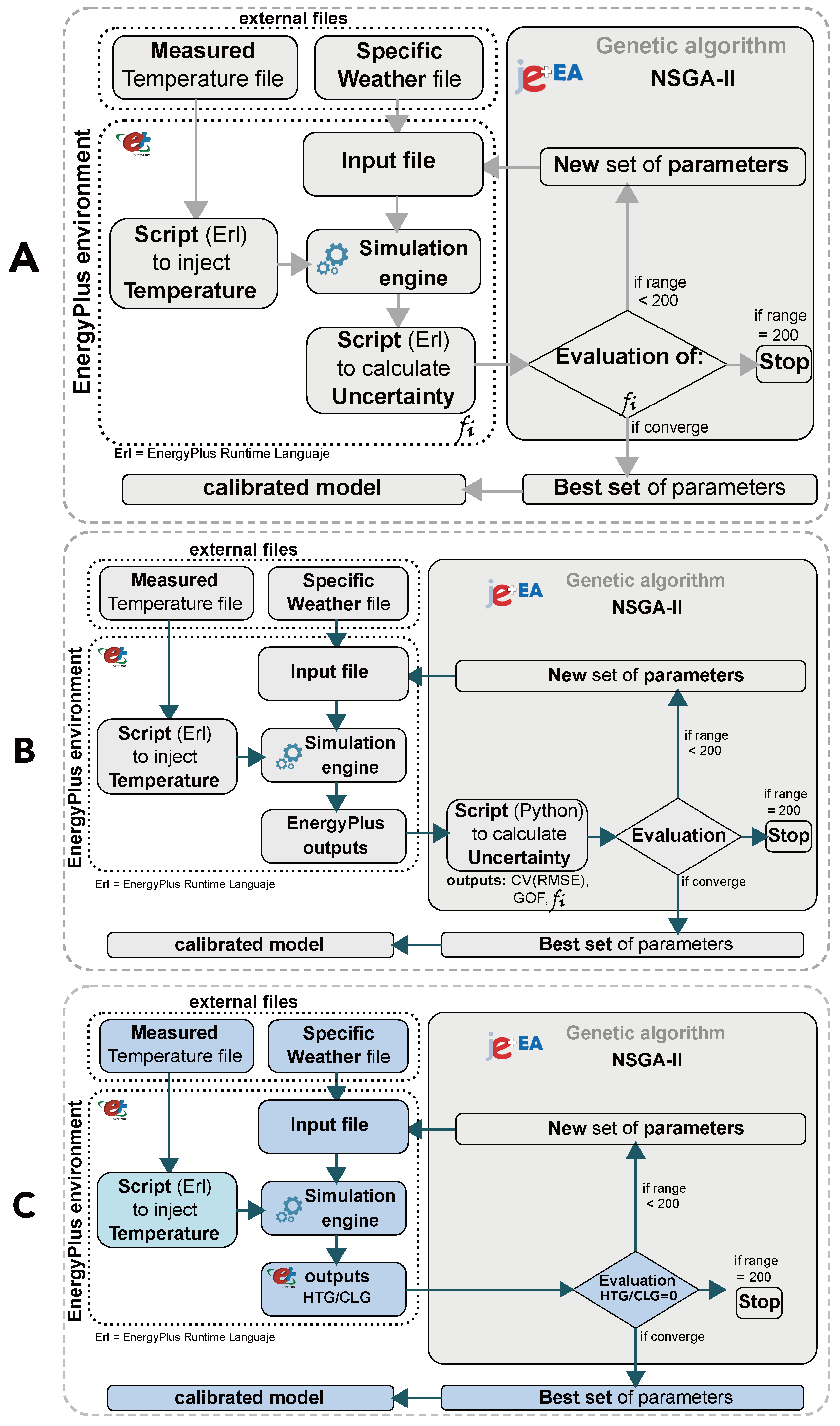
From our point of view, the criteria for considering whether or not a calibrated model is data-driven should rely on the use made of the measured data that will be introduced in the model. In most of the automatic calibration techniques, the data are not part of the calibration process (except for the weather data file). The simulated data are used at the end of the simulation to be compared against measured data. This comparison is called uncertainty analysis, and the results of the uncertainty analysis are used as an objective function by the algorithm to select a new set of parameters or otherwise. This idea can be seen graphically in Figure 1B.

This means that measured data is not part of the models’s energy balance equation [28,29,30,31]. The reason is that programs such as EnergyPlus and TRNSYS have severe problems with the initialization of variables [22], and it is difficult to introduce data that could affect the thermal energy balance. Because of this issue, most calibration techniques based on a whole building simulation programs use the data at the end of the process as a comparison between simulated and measured data. From a practical point of view, it means that the measured data does not influence the energy balance of the thermal zone [18,19,24,32,33,34,35,36,37].

This is a problem that we have partially solved before [26,27], because our methodology reproduces the thermal history of the building as a dynamic set-point. It is an external comma-delimited file with the temperature data taken from the real building that will be introduced as the set-point thermostat. The goals of these files are pre-heating or pre-cooling the building before the calibration process starts. Accordingly, we can introduce as much measured data (temperatures) as needed. In fact, the more zones that are included the better, because these data increase the thermal characterization of the model. A problem remains, however, due to the fact that we have to stop the dynamic set-point at the time of starting the calibration process, because otherwise the indoor temperature would be useless in the uncertainty analysis.

By maintaining the dynamic set-point all the time, we would not lose the thermal history of the building during the free floating period. The question that arises then is whether it is possible to maintain the thermal history while the calibration process is in progress.

This is the main novel contribution of this article: we present an easier objective function that gives a powerful stimulus to the algorithm and allows the maintenance of the dynamic set-point during the calibration process.

This new objective function is the energy consumed to maintain the dynamic set-point temperature of the thermal zone in free oscillation mode. This energy should ideally be zero if the model has the right envelope parameters. On the other hand, if the parameters of the envelope are not correct, this energy consumption will be very high and the algorithm will discard that set because it does not comply with the requirements of being zero. We have called this methodology zero energy for calibration (ZEC) because we are looking for a zero energy objective. The concept is simple and the results are very good, as be seen in Section 3.

The new methodology we propose simplifies the previous two methodologies, as shown in Figure 1. The first and second approaches were based on uncertainty calculations. The first one [27] used an internal object of EnergyPlus (Energy Management System—EMS) to calculate the uncertainty of the model (see Figure 1A). The second [26] simplified the methodology using a script developed in Python, enabling the user to divide the model into all of the thermal zones needed (see Figure 1B). This new methodology uses a direct output of EnergyPlus, reducing the complexity of the process and achieves this, more importantly, without losing the thermal history of the building.

3. The Design of the Experiment

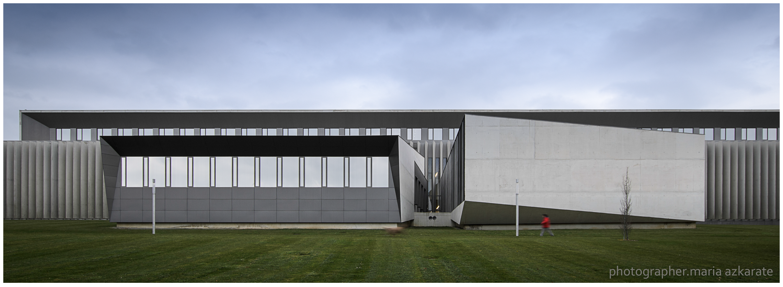
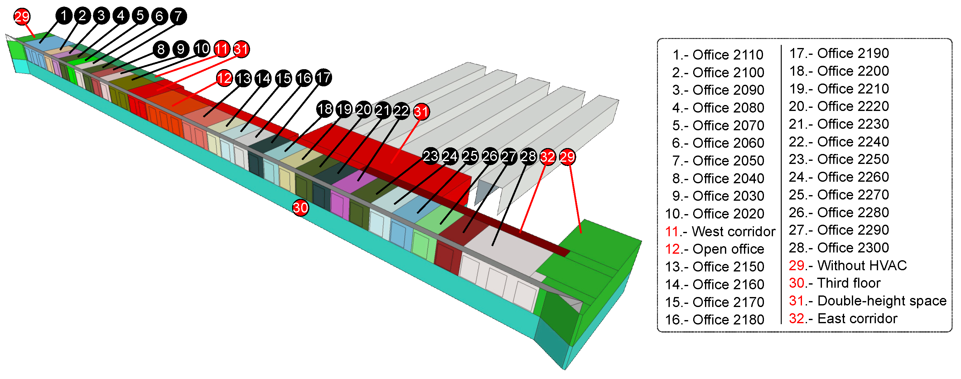
As in our past two articles [26,27], the building under consideration is the “Amigos” building in the University of Navarra (see Figure 2). The model used is the same as in the second article [26], with 32 thermal zones (see Figure 3). Finally, in order to compare the three different methodologies, all of the data measured (the temperature, weather, and blower door test [38]) have been reused.

This approach is very similar to the other methodologies, and includes the use of a genetic algorithm (GA), non-dominated sorting genetic algorithm II (NSGA-II) [39,40,41], to find calibrated BEMs in the search space defined by the parameters shown in

Table 1. Search space for the genetic algorithm.

	Construction	Type of Parametrized Value	Baseline Model	Other Values
			Value 1	Value 2	Value 3	Value 4	Value 5	Value 6	Value 7	Value 8	Value 9	Value 10
A	Façade CE04c	Thickness (m)	0	0.05	0.06	0.07	0.08	0.09	0.1	0.11	-	-
B		Brick density (kg/m3)	1150	1250	1350	1450	1550	-	-	-	-	-
C	Façade CE06a	Thickness (m)	0	0.01	0.02	0.03	0.04	0.05	0.6	0.07	-	-
D	Façade CE06b	Thickness (m)	0	0.05	0.06	0.07	0.08	0.09	0.1	0.11	-	-
E	Façade CE07	Thickness (m)	0	0.05	0.06	0.07	0.08	0.09	0.1	0.11	-	-
F	Roof	Insulation thickness (m)	0.10	0.15	0.20	0.25	0.30	0.35	0.40	0.45	0.50	0.55
G		Gravel thickness (m)	0.10	0.025	0.05	0.075	0.125	0.15	0.175	0.20	-	-
H	Top façade	Thickness (m)	0	0.01	0.02	0.03	0.04	0.05	0.6	0.07	-	-
I	Slab	Specific heat (J/kgK)	1000	850	900	950	1050	1100	-	-	-	-
J		Thickness (m)	0.35	0.25	0.30	0.40	0.45	0.50	-	-	-	-
K	Partition walls	Density (kg/m3)	1	1000	1100	1200	1300	1400	1500	1600	1700	-
L	U-Factor	W/m2K	1.4	0.8	0.9	1.0	1.1	1.2	1.3	-	-	-
M	Solar Heat Gain Coefficient	Non-dimensional	0.6	0.4	0.5	0.7	0.8	0.9	1.0	-	-	-

. The genetic algorithm is one of the metaphor-based methods of metaheuristic algorithms. It is based on Darwin’s theory of evolution, where in each iteration (generation) a set of simulations (population) is generated. The best individuals of the population are the ones that best match with the objective function, and therefore they must survive (the survival principle). Thanks to the crossover (switch parent’s simulations) and mutation (random parameter changes) operators, the generated offspring preserve the good attributes of the parents. As in the other article [27], the population size is 10 and the maximum value of generations is 200. These values are taken from the author’s experience, as we are using the same search space 1.07 × 10²¹. With bigger search spaces, the number of generations and the population size should be considered. The use of the new objective function (ZEC) simplifies the energy model used and allows the maintenance of the dynamic thermal history of the building throughout the whole calibration process (see Figure 1A–C).

The idea behind this experiment is to show that the methodology we are proposing now is robust and consistent and can therefore be applied in a general context.

As in the other automatic calibration techniques, the uncertainty analysis allows an evaluation of the model with well-known statistical indices such as coefficient of determination ($R^2$), coefficient of variation of the root mean square error ($CV\left(RMSE\right)$), and normalized mean bias error ($NMBE$) [42]. ASHRAE Guidelines 14 [43,44], Federal Energy Management Program (FEMP) 3.0 [45,46], and International Performance Measurements and Verification Protocol (IPMVP) [3] recommend limits in order to consider an energy model as calibrated.

Table 2. Calibration criteria of the Federal Energy Management Program (FEMP), ASHRAE Guideline 14 and IPMVP. $CV\left(RMSE\right)$: coefficient of variation of the root mean square error; IPMVP: International Performance Measurements and Verification Protocol; $NMBE$: normalized mean bias error.

Data Type	Index	FEMP Criteria [45,46]	ASHRAE Guideline 14 [43,44]	IPMVP [3]
Calibration criteria
Monthly criteria %	$NMBE$	±5	±5	±20
	$CV\left(RMSE\right)$	15	15	-
Hourly criteria %	$NMBE$	±10	±10	±5
	$CV\left(RMSE\right)$	30	30	20
Model recommendation
	$R^2$	-	>0.75	>0.75

shows the limits of the different documents. When the statistical indices are used as an objective function, these are embedded in the calibration process. In our case, we did not use this approach; as a result, this analysis must be performed at the end of the simulation to check if the values are within the limits according to Table 2.

The main purpose of this article is the demonstration of a new methodology in the field of building calibration. We have taken advantage of our previous articles, as well as the calibrated model that was produced before. With this methodology, however, we can easily reach the same level of calibration quality demonstrated in the previous work, with an important reduction in the degree of complexity. We have performed the calibration in different scenarios with the purpose of showing that it is possible to produce high-quality calibrated models in all of them despite the fact that some have a reduced quantity of data (see Figure 4).

We propose a four-stage process to carry out the methodology:

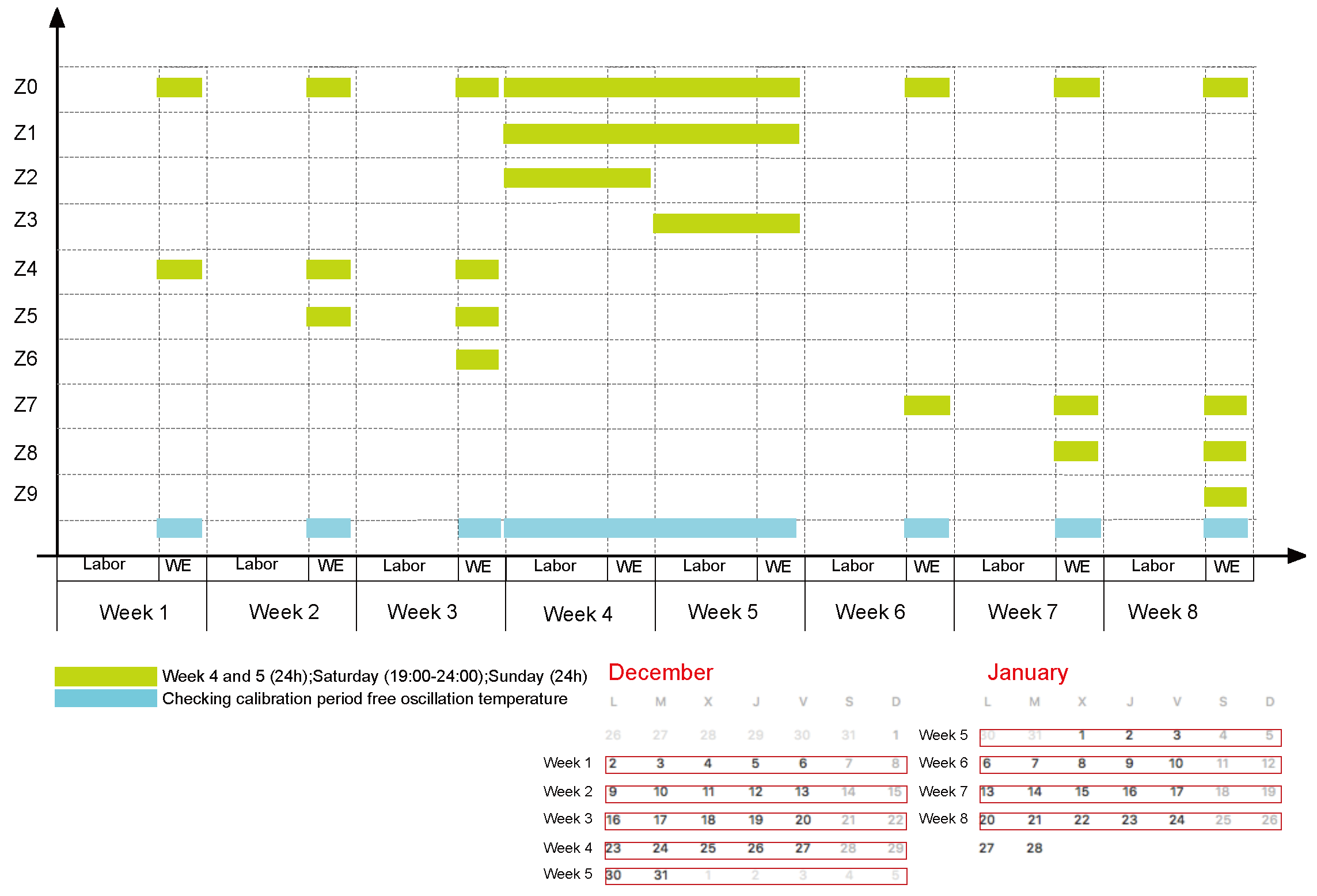
• First stage: Select a variety of different periods with temperature data available in free oscillation mode. Free oscillation periods are very suitable for achieving good calibration results when we are trying to find good parameters for the building envelope. Figure 4 shows the schema and the names proposed for the different periods. Each scenario has been named from $Z0$ to $Z9$. The idea is to check if the methodology we propose can offer reliable results in different environments. Each scenario ($Z0,Z1,\dots ,Z9$) will produce a class of models ($M0,M1,\dots ,M9$). The calibration process is guided by the genetic algorithm (NSGA-II), and since it is a stochastic approach, there are several solutions. For each class, we have chosen the first 20 models ($M0\_00,M0\_01,\dots ,M1\_19$). In order to compare this new methodology with the former one [26], the results of our past calibration study have been included as an extra class named as “R” ($R\_01,R\_02,\dots ,R\_20$). Thus, the total amount of models that we are going to check is 220.
  In relation to the different periods, we can comment that $Z0$ is the longest scenario. This scenario has a double function, as a space of calibration and at the same time as a space for checking for the rest of the models. This means that all the models will be evaluated in this scenario independently of where they have been generated. This scenario has been used in our previous articles [26,27]. In this way, we can compare all the models under the same conditions.
  We can divide the rest of the scenarios into three types. The first three ($Z1$, $Z2$, and $Z3$) are related to the long period of the Christmas season (week 4 and 5) where the building was unoccupied and out of operation. The first type covers the whole period, and the other two are the first and second halves of this period. The second type corresponds with the previous weekends. In particular, $Z6$ is a very challenging scenario where we use data from one weekend, but must take note that the weekend is formed by 30 h of temperature data taken at a pace of ten minutes per time-step. The third type is similar to the previous one, but with the difference that the building structure is cold after the unoccupied period, and therefore a transient state of heat storage is generated.
• Second stage: In this phase we prepare the EnergyPlus models for producing energy, heating (HTG), and cooling (CLG) for those periods. This information will be introduced into the GA as an objective function (Figure 1C), and the goal will be to obtain the least possible amount of energy (ideally zero). Our approach is that the model that provides a better fit to the measured curve of temperature with the least amount of energy is the one nearer to the real model.
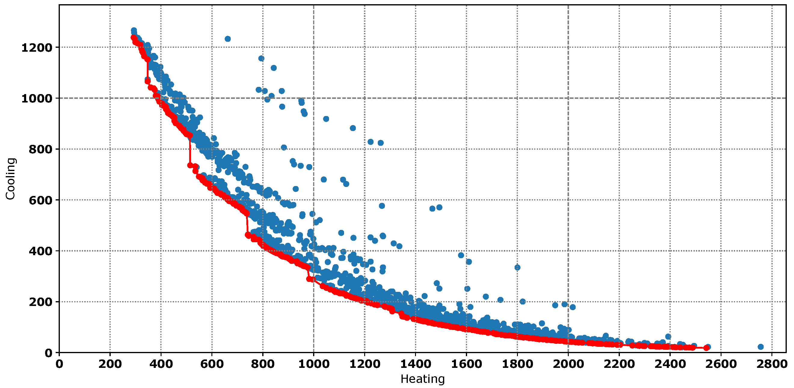
• Third stage: We perform the genetic algorithm in order to determine the parameters that produce lower energy. As can be seen in Figure 5, the objective function obeys the classical rule of a Pareto front (red dots), because we are working with a pair of values (heating and cooling) that are opposite. The algorithm used to perform the thermal zone energy balance in EnergyPlus is the conduction transfer function (CTF), which offers a very fast an elegant solution to find the temperature of the thermal zone. However, zero energy calibration (ZEC) is a technique based on the thermal zone energy balance, and for that reason, CTF sometimes introduces energy penalty. This extra energy consumption makes it so that some models with slightly higher energy consumption have better uncertainty results than the best models ranked by energy. Therefore, the best way of solving this problem is by selecting the 20 best energy models, in the same way as other similar works [47].
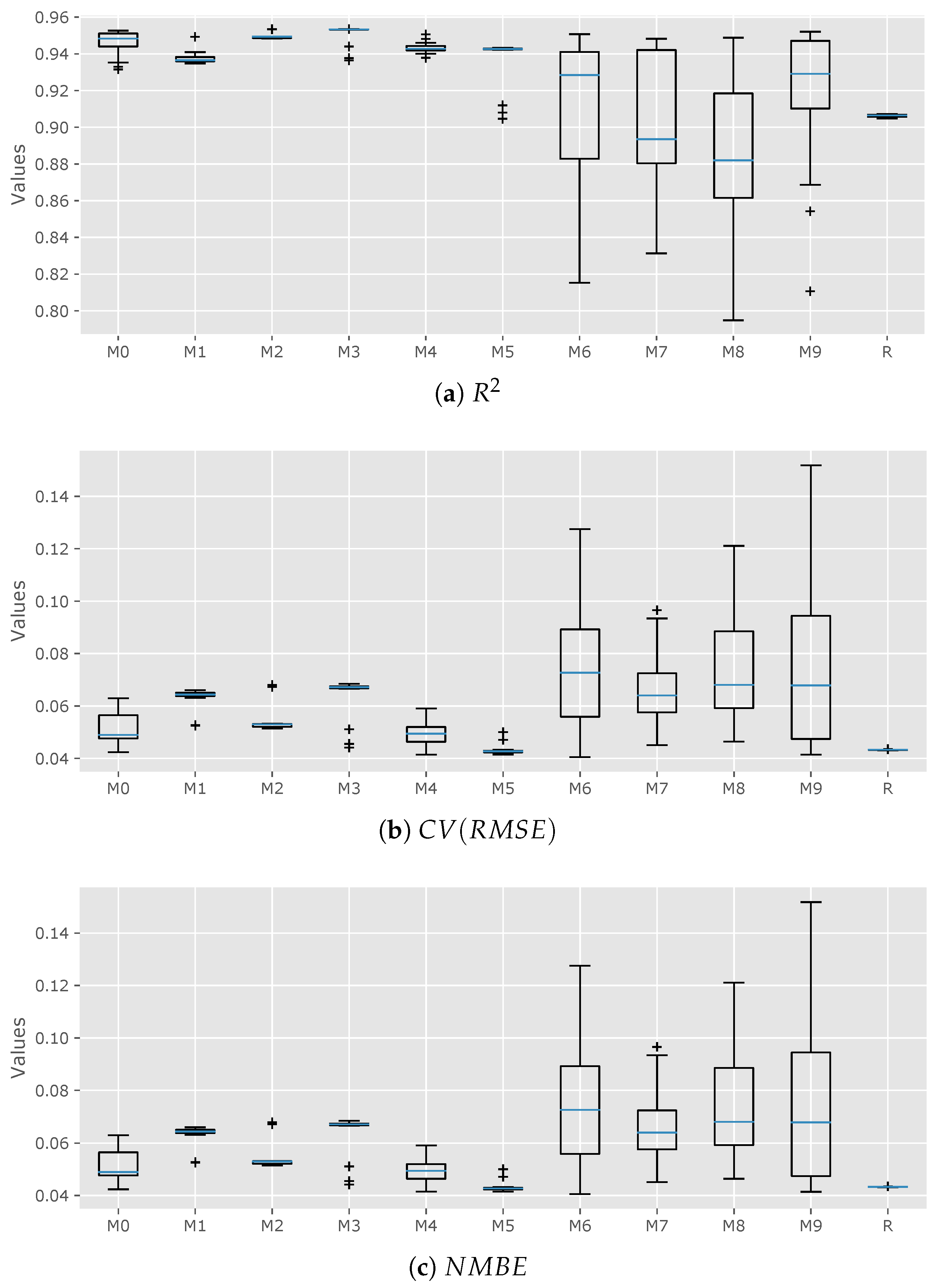
• Fourth stage: Once the 20 best models of each class ($M0,M1,\dots ,M9$) have been selected, we perform an uncertainty analysis to check if the results of the calibration process are within the margins recommended by ASHRAE Guidelines 14, FEMP 3.0, and IPMVP (see Table 2). We have used the box plot graph see Figure 6 as a way of measuring the dispersion or compactness of the models. In general, we can state that when a model’s class offers compact values, the calibration process is clear on that zone, and when there is dispersion, more attention should be paid. This could mean ($M0,M1,\dots ,M9$) that the algorithm has insufficient data to offer a compact solution. The last statement does not mean that good results cannot be achieved, as will be seen later in this article.

4. Analysis of the Results

The results offered by Figure 6 are coherent and have improved the quality of those obtained in the past [26]. Each figure offers its own range of values, but the results have a similar pattern, which is commented upon below.

First, the models generated in the weeks prior to Christmas ($M4$, $M5$, and $M6$) and during the Christmas period ($M1$, $M2$, and $M3$) offer very compact data; the former produces good results in terms of $R^2$, $NMBE$, and $CV\left(RMSE\right)$, and the latter generates results that comply with calibrating criteria in Table 2. It is remarkable that the models that have been calibrated with data taken from one weekend ($M6$ and $M9$)—despite having disperse values among their ranks—give very good results.

The dispersion in models $M7$ and $M8$ could be related to the cold building phenomenon. This means that during those days the building was storing energy after the unoccupied weeks and its thermal behavior was transient, in contrast with models $M4$ and $M5$ that were generated in more steady-state conditions. This phenomenon could have finished in the third weekend after unoccupied weeks, which could be the reason why model $M9$ demonstrated very good results. The same dispersion pattern can be observed in Figure 6 in terms of the $R^2$, $CV\left(RMSE\right)$, and $NMBE$ analysis.

For a better understanding of the results, we have generated several

Table 3. Rank of models. Ranks distribution.

Class	Best Rank	Rank-25	Rank-50	Rank-75	Rank-100
$M0$	5	2	13	14	14
$M1$	151	0	0	0	0
$M2$	74	0	0	2	18
$M3$	129	0	0	0	0
$M4$	3	1	7	10	14
$M5$	2	20	20	20	20
$M6$	1	1	5	5	6
$M7$	31	0	1	2	3
$M8$	62	0	0	2	2
$M9$	4	1	4	5	6
R	53	0	0	15	17
Total		25	50	75	100

,

Table 4. Rank of models. The best models.

Rank	Class	${\mathit{R}}^2$	$\mathit{NMBE}$	$\mathit{CV}\left(\mathit{RMSE}\right)$	Index
1	$M6$	92.281%	0.436%	4.053%	0.12203
2	$M5$	94.223%	2.311%	4.152%	0.12235
3	$M4$	94.084%	2.238%	4.146%	0.12296
4	$M9$	94.027%	2.198%	4.143%	0.12310
5	$M0$	94.399%	2.531%	4.237%	0.12365
6	$M5$	94.273%	2.439%	4.212%	0.12373
7	$M5$	94.219%	2.397%	4.202%	0.12375
8	$M5$	94.246%	2.420%	4.208%	0.12377
9	$M5$	94.256%	2.438%	4.216%	0.12393

and

Table 5. Rank of models. The best of each class.

Class	Best Rank	${\mathit{R}}^2$	$\mathit{NMBE}$	$\mathit{CV}\left(\mathit{RMSE}\right)$	Index
$M0$	5	94.399%	2.531%	4.237%	0.12365
$M1$	151	93.154%	4.763%	6.061%	0.17670
$M2$	74	94.839%	3.951%	5.140%	0.14252
$M3$	129	95.321%	5.835%	6.652%	0.17166
$M4$	3	94.084%	2.238%	4.146%	0.12296
$M5$	2	94.223%	2.311%	4.152%	0.12235
$M6$	1	92.281%	0.436%	4.053%	0.12203
$M7$	31	93.631%	2.403%	4.456%	0.13227
$M8$	62	91.855%	1.208%	4.677%	0.14030
$M9$	4	94.027%	2.198%	4.143%	0.12310
R	53	90.463%	0.065%	4.360%	0.13962

. In Table 3 it is intended that it is clear to see for each class ($M0,M1,\dots ,M9$ and R) which are the best models of the 220 that have been analyzed and how they are distributed in quality. Therefore, “Best rank” shows the position in the ranking of the best models which is the best of each class. $M6$ is the best, with number one. “Rank-25” indicates the number of models in each class that are between the 25 best models. $M5$ is the second in Best rank and has the 20 best models among the best. In contrast, the best one among the ranks ($M6$) has only one in the “Rank-25”. This means that on the one hand, the calibration space $Z5$ produced very good results in all the models, but on the other hand, the $Z6$ space has the capacity of producing good results but does not always do so. Something similar happens to class $M9$. “Rank-50” demonstrates the same analysis but does so between the 50 best models, and so on.

Table 4 offers the results ordered by index parameter. The index parameter is obtained as the arithmetic sum of the errors ($CV\left(RMSE\right)$, $NMBE$, and $R^2$). The $R^2$ error is achieved by subtracting 1 from the value. The model with the lowest index is the one considered to have the best performance. The different columns show the uncertainty index of each model, and as can be seen, all of them comply with the requirements of ASHRAE Guideline 14, FEMP 3.0, and IPMVP. It is surprising to see that the best model was produced in one of the more challenging calibration spaces ($Z6$, the one with 30 h of measured data), and another model from $Z9$ is in fourth place.

In Table 5 we want to show that even models that have very high ranks such as $M1,M2,M3$, and $M8$ are calibrated when they are contrasted with ASHRAE Guidelines 14, FEMP 3.0, and IPMVP parameters in Table 2.

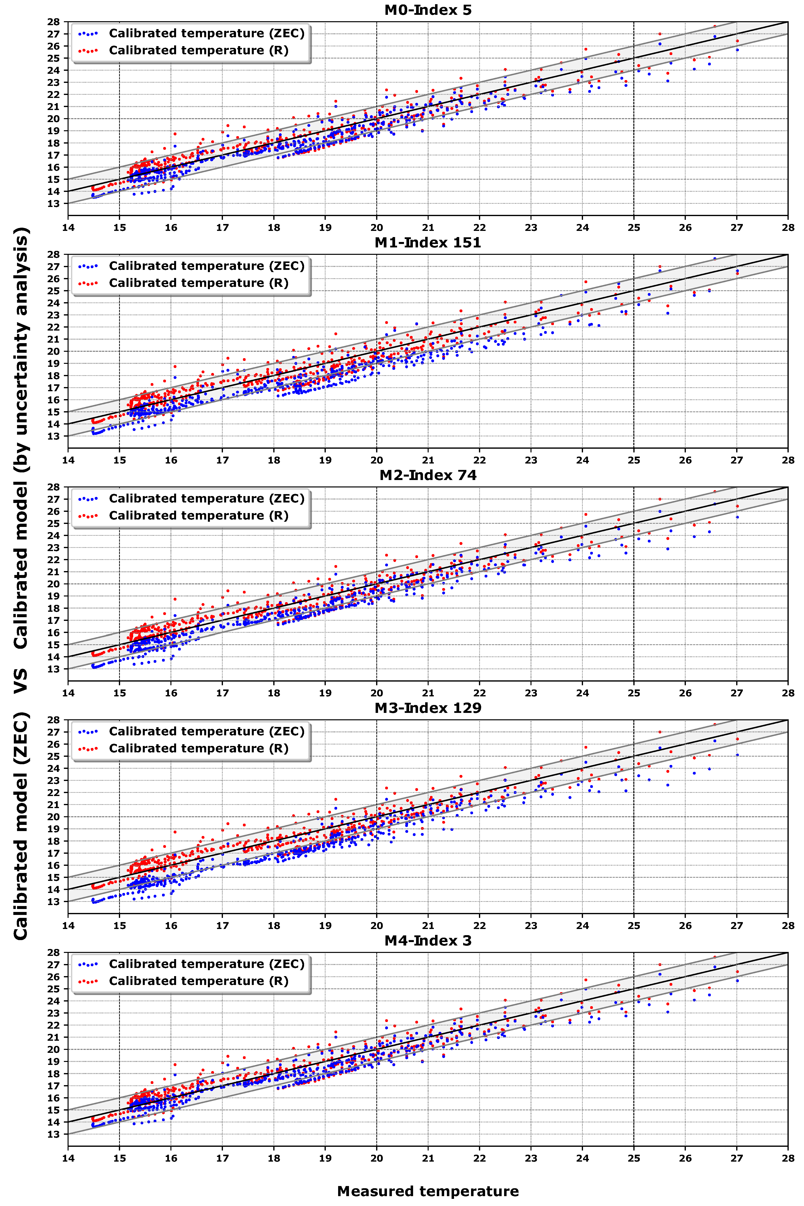
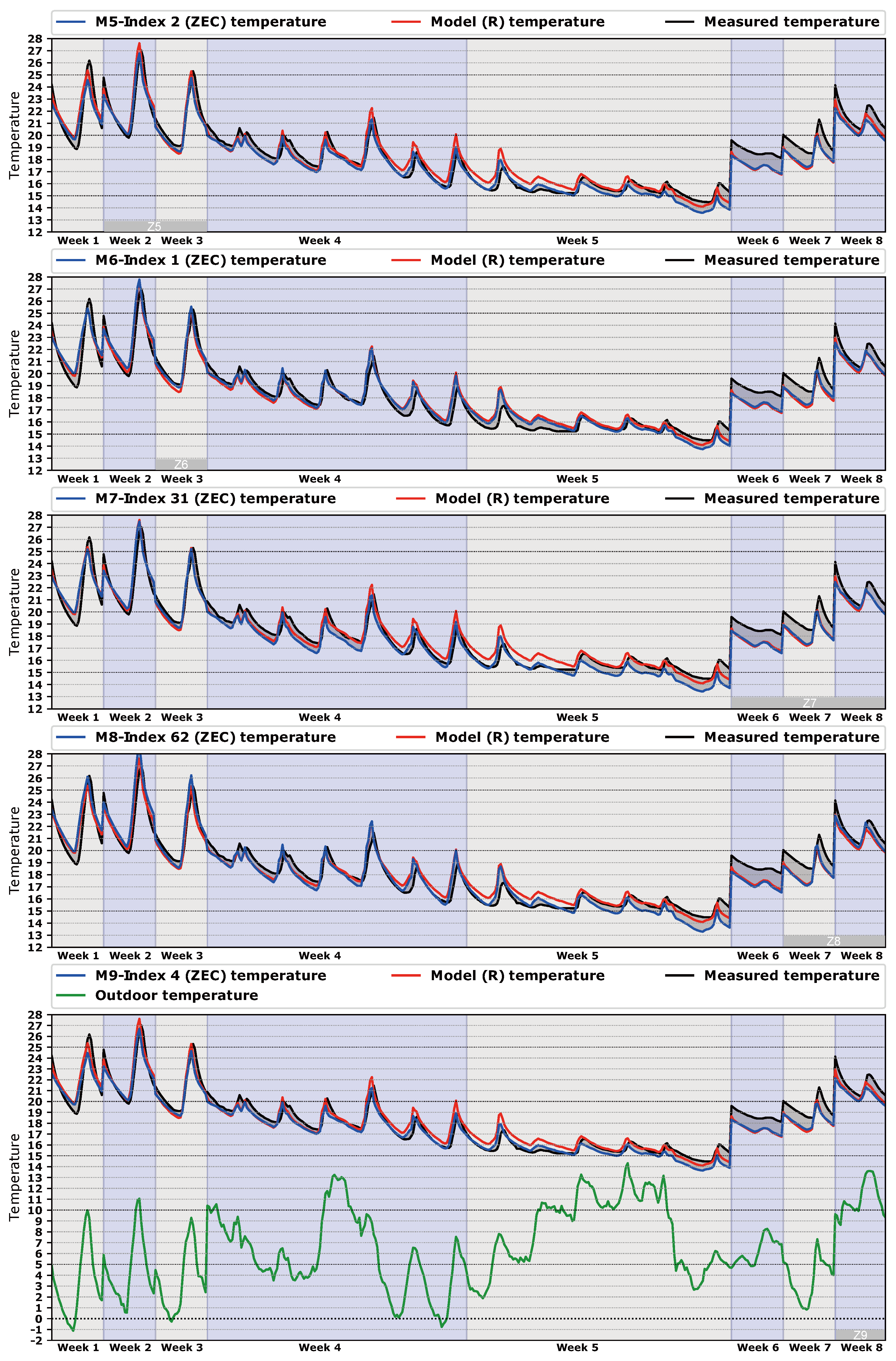
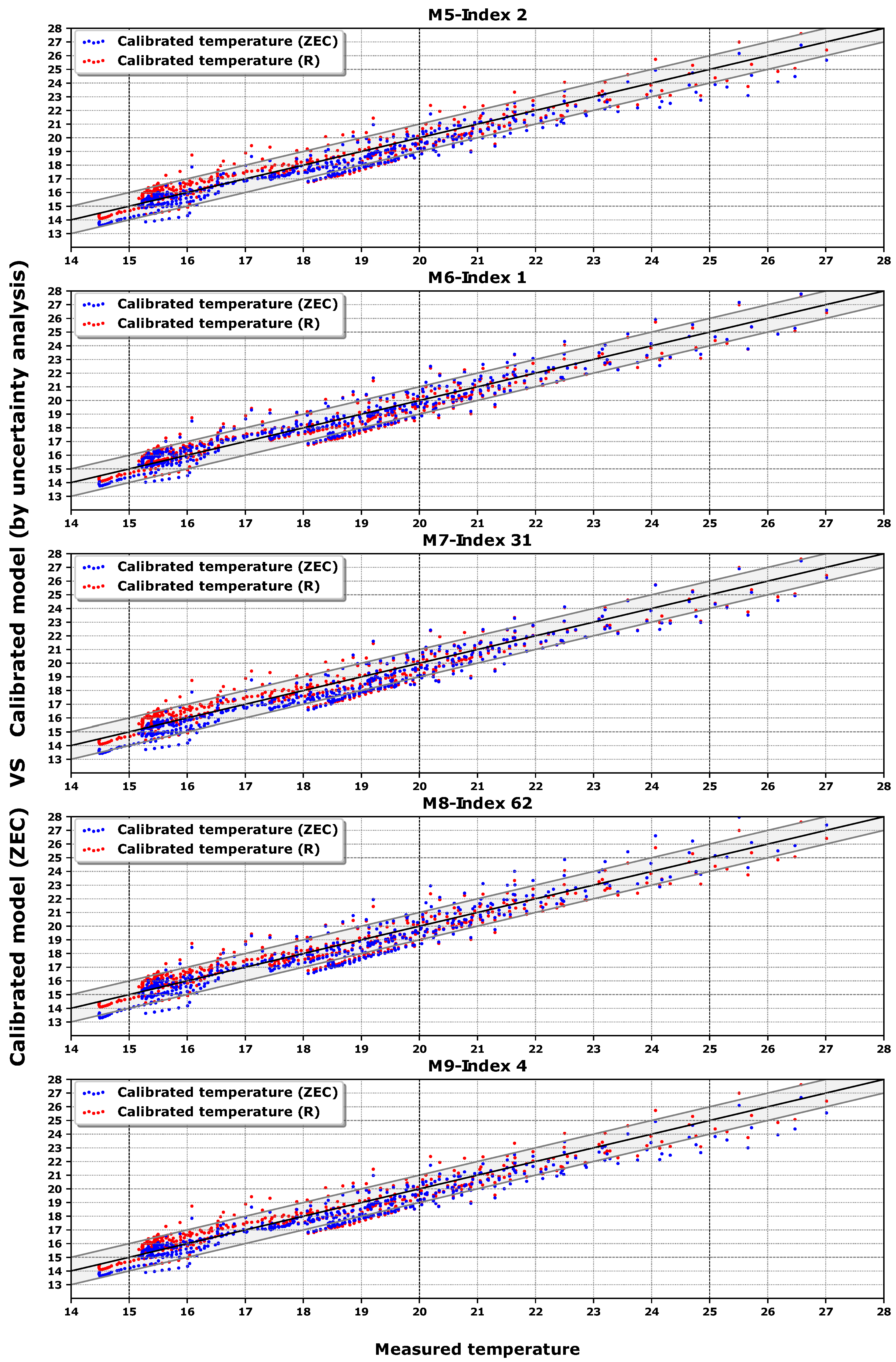
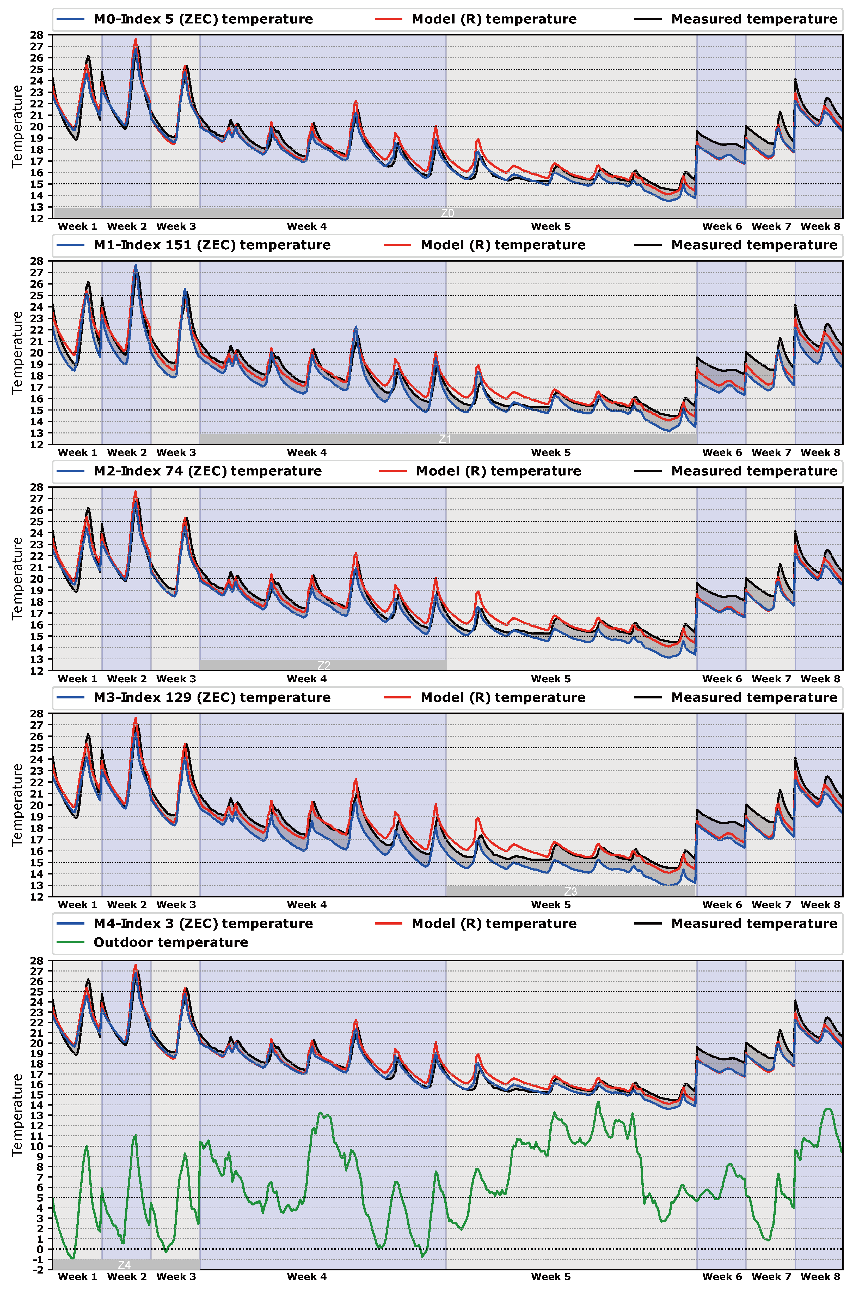
Finally, we show the data from Table 5 in a series of temperature dispersion graphs in Figure 7 and in temperature time series in Figure 8 . The best model of each class is compared with the best model of class R, which was classified in rank 53 according to the Index in Table 5. In this way, we intend to check the quality of the new methodology over the last [26]. In the dispersion graphs of Figure 7, a band of $\pm 1$ ${}^{\circ }$C shows the accuracy of the calibration process. Each dot represents the hourly average free oscillation temperature inside the building; there are 466 h of comparison. Figure 8 represents the same temperatures, but organized by the time in which they were generated. In this way, we can see the relation between temperatures and spaces of calibration ($Z0$, $Z1$, …, $Z9$), as can be seen in Figure 8. Extra information such as outdoor temperature, measured temperature, and temperature of the best model of class R is exposed in Figure 8 for a better understanding of the process.

Some observations can be noted from Figure 7 and Figure 8. First, as the measured temperature has mainly been taken with the building unoccupied (free oscillation), it tends to be cooler. This calibration methodology based on energy works better with a greater thermal jump between indoor and outdoor temperature. These lower temperatures were generated in week 5, as can be seen in Figure 8. Moreover, in week 5 the outdoor temperature increased suddenly and therefore the jump between outdoor and indoor temperatures decreased. This presents a problem, because the lower the thermal jump, the lower the energy available by the algorithm to find a set of more suitable parameters.

Secondly, the results can be organized into three kinds of models:

• Models that perform better than the best R model ($M0$, $M4$, $M5$, $M6$, $M9$). If we look at them from the point of view of the time taken for calibration, three types can be considered: long calibration spaces like $Z0$ with 466 h of free oscillation, medium spaces like $Z4$ and $Z5$ with 90 h and 60 h, respectively, and short calibration spaces like $Z6$ and $Z9$ with 30 h. The common characteristic of these spaces is that the indoor temperature is generally over 20 ${}^{\circ }$C, and therefore they are the warmer free oscillation hours of the process. Accordingly, we can state that during these free oscillation hours the building is thermally in a steady-state condition.
• Models that perform similarly to the R model ($M2$, $M7$, $M8$). In this case, the spaces $Z2$, $Z7$, and $Z8$ have 143, 90, and 60 h of calibration, respectively. They have in common a mixture of warm and cool indoor temperatures, due to the proximity to week 5. This week generates a bad influence in the calibration process that reduces the quality of the models, as we have said before. Hence, we can say that in these zones the building is thermally in a transient state from a warm to cool period ($M2$) and from a cool to a warm period ($M7$, $M8$).
• Models that perform worst than the best R model ($M1$, $M3$). It seems clear that the reason for that is because week 5 is part of the calibration space. As we have said before, in this week the junction of two phenomena (low indoor temperature and high outdoor temperature) generated a low thermal jump, which produces poor results.

5. Conclusions

The basis of this technique is the thermal characterization of the building. This means that the model is guided through the same thermal path as the real building. This idea opens the door to new possibilities for calibration techniques with different objective functions, both statistical and physical.

As can be seen in Figure 1, this procedure is very easy to implement. The software is available for download and is user-friendly, and from the hardware point of view, a standard PC is enough to run the simulations. The outputs of heating and cooling are standard values of EnergyPlus, and the coupling with the optimization software (jEPlus + EA [48]) does not present any problem. The main difficulty is the data gathering (temperature) and the work of generation schedules to feed the set-points. We have solved this problem via energy management system (EMS). Other options (e.g., via MATLAB) can be used for doing that work [17].

The main conclusions of this article are:

• The simplicity of implementing new calibration spaces with a reduced amount of data (temperature).
• There is no need to have long free oscillation periods in order to produce good results in terms of $R^2$, $NMBE$, and $CV\left(RMSE\right)$.
• A dramatic reduction in the expertise and the amount of code needed to implement a reliable model is realized. It means that the code to connect the simulation environment with the optimization software has disappeared.
• In this new approach, the temperatures measured in each thermal zone are the guide for the algorithm to find a suitable set of parameters. Therefore, the new methodology takes advantage of a complete thermal characterization of the model.
• The proposed methodology has the limitation that the measured data should be gathered from an unoccupied building.

This new idea of a law-data-driven model allows us to use all of the data measured in the real building for the calibration process. We can take advantage of the power calculation capacity of the whole energy simulation program to reduce the gap between the model and the real building.

6. Future Works

The high level of quality obtained for this model—in comparison with the standards of ASHRAE Guidelines 14, FEMP 3.0, and IPMVP—encourages us to think that the model could go beyond a mere energy evaluation or prediction of future building energy performance. The question remains as to whether we can use this model as virtual monitoring. Improvements to the algorithm are also needed in order to reduce the calibration time, which is around 20 h in a 2-core machine and 3 h in a 16-core machine. Other objective functions (statistical and physical) will be developed in the future to enable calibration in unoccupied periods. More case studies should be developed to test how this new calibration procedure will work in other situations that could have a greater impact than the parameters selected in this case study, such as phase change materials [49], cool roofs [50], etc.